Spatially Distributed Sampling and Reconstruction

Abstract.

A spatially distributed system contains a large amount of agents with limited sensing, data processing, and communication capabilities. Recent technological advances have opened up possibilities to deploy spatially distributed systems for signal sampling and reconstruction. In this paper, we introduce a graph structure for a distributed sampling and reconstruction system by coupling agents in a spatially distributed system with innovative positions of signals. A fundamental problem in sampling theory is the robustness of signal reconstruction in the presence of sampling noises. For a distributed sampling and reconstruction system, the robustness could be reduced to the stability of its sensing matrix. In a traditional centralized sampling and reconstruction system, the stability of the sensing matrix could be verified by its central processor, but the above procedure is infeasible in a distributed sampling and reconstruction system as it is decentralized. In this paper, we split a distributed sampling and reconstruction system into a family of overlapping smaller subsystems, and we show that the stability of the sensing matrix holds if and only if its quasi-restrictions to those subsystems have uniform stability. This new stability criterion could be pivotal for the design of a robust distributed sampling and reconstruction system against supplement, replacement and impairment of agents, as we only need to check the uniform stability of affected subsystems. In this paper, we also propose an exponentially convergent distributed algorithm for signal reconstruction, that provides a suboptimal approximation to the original signal in the presence of bounded sampling noises.

1. Introduction

Spatially distributed systems (SDS) have been widely used in (underwater) multivehicle and multirobot networks, wireless sensor networks, smart grids, etc ([2, 19, 23, 74, 75]). Comparing with traditional centralized systems that have a powerful central processor and reliable communication between agents and the central processor, an SDS could give unprecedented capabilities especially when creating a data exchange network requires significant efforts (due to physical barriers such as interference), or when establishing a centralized processor presents the daunting challenge of processing all the information (such as big-data problems). In this paper, we consider SDSs for signal sampling and reconstruction, and we describe the topology of an SDS by an undirected (in)finite graph

(1.1) $${\mathcal{G}}:=(G,S),$$

where a vertex represents an agent and an edge between two vertices means that a direct communication link exists.

In the SDS described above, sampling data of a signal $f$ acquired by the agent $\lambda\in G$ is

(1.2) $$y(\lambda):=\langle f,\psi_{\lambda}\rangle,$$

where $\psi_{\lambda}$ is the impulse response of the agent $\lambda\in G$ ([4, 7, 8, 32, 48, 57, 59, 70, 71, 72]). Fundamental signal reconstruction problems are whether and how the signal $f$ can be recovered from its sampling data $y(\lambda),\ \lambda\in G$. For well-posedness, the signal $f$ of interest is usually assumed to have additional properties, such as band-limitedness, finite rate of innovation, smoothness, and sparse expansion in a dictionary ([7, 15, 26, 27, 28, 71, 72]). In this paper, we consider spatial signals with the following parametric representation,

(1.3) $$f:=\sum_{i\in V}c(i)\varphi_{i},$$

where amplitudes $c(i),i\in V$, are bounded, and generators $\varphi_{i},i\in V$, are essentially supported in a spatial neighborhood of the innovative position $i$. The above family of spatial signals appears in magnetic resonance spectrum, mass spectrometry, global positioning system, cellular radio, ultra wide-band communication, electrocardiogram, and many engineering applications, see [27, 61, 72] and references therein.

In this paper, we associate every innovative position $i\in V$ with some anchor agents $\lambda\in G$, and denote the set of such associations $(i,\lambda)$ by $T$. These associations can be easily understood as agents within certain (spatial) range of every innovative position. With the above associations, we describe our distributed sampling and reconstruction system (DSRS) by an undirected (in)finite graph

(1.4) $${\mathcal{H}}:=(G\cup V,\ S\cup T\cup T^{*}),$$

where $T^{*}=\{(\lambda,i)\in G\times V,\ (i,\lambda)\in T\}$, see Figure 1. The above graph description of a DSRS plays a crucial role for us to study signal sampling and reconstruction.

Given a DSRS described by the above graph ${\mathcal{H}}$, set

(1.5) $$E:=\{(i,i^{\prime})\in V\times V,\ \ i\neq i^{\prime}\ {\rm and}\ (i,\lambda),(i^{\prime},\lambda)\in T\ {\rm for\ some}\ \lambda\in G\}.$$

We then generate a graph structure

(1.6) $${\mathcal{V}}:=(V,E)$$

for signals in (1.3), where an edge between two distinct innovative positions in ${V}$ means that a common anchor agent exists. The above graph structure for signals is different from the conventional one in most of the literature, where the graph is usually preassigned. The reader may refer to [52, 53, 56] and Remark 3.6.

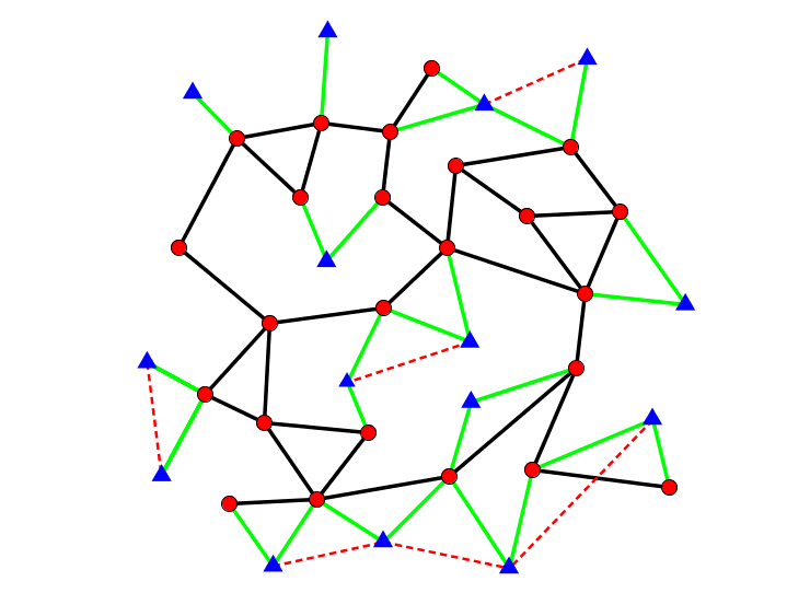
Figure 1. The graph ${\mathcal{H}}=(G\cup V,\ S\cup T\cup T^{*})$ in (1.4) to describe a DSRS, where vertices in $G$ and $V$ are plotted in red circles and blue triangles, and edges in $S,T$ and $E$ are in black solid lines, green solid lines and red dashed lines respectively.

Define sensing matrix ${\bf S}$ of our DSRS by

(1.7) $${\bf S}:=(\langle\varphi_{i},\psi_{\lambda}\rangle)_{\lambda\in G,i\in V}.$$

The sensing matrix ${\bf S}$ is stored by agents in a distributed manner. Due to the storage limitation, each agent in our SDS stores its corresponding row (and perhaps also its neighboring rows) in the sensing matrix ${\bf S}$, but it does not have the whole matrix available. Agents in our SDS have limited acquisition ability and they could essentially catch signals not far from their physical locations. So the sensing matrix ${\bf S}$ has certain polynomial off-diagonal decay, i.e., there exist positive constants $D$ and $\alpha$ such that

(1.8) $$|\langle\varphi_{i},\psi_{\lambda}\rangle|\leq D(1+\rho_{\mathcal{H}}(\lambda,i))^{-\alpha}\ {\rm for\ all}\ \lambda\in G\ {\rm and}\ i\in V,$$

where $\rho_{\mathcal{H}}$ is the geodesic distance on the graph ${\mathcal{H}}$. For most DSRSs in applications, such as multivehicle and multirobot networks and wireless sensor networks, the signal generated at any innovative position could be detected by its anchor agents and some of their neighboring agents, but not by agents in the SDS far away. Thus the sensing matrix ${\bf S}$ may have finite bandwidth $s\geq 0$,

(1.9) $$\langle\varphi_{i},\psi_{\lambda}\rangle=0\quad{\rm if}\ \rho_{\mathcal{H}}(\lambda,i)>s.$$

The above global requirements (1.8) and (1.9) could be fulfilled in a distributed manner.

The sensing matrix ${\bf S}$ characterizes the sampling procedure (1.2) of signals with the parametric representation (1.3). Applying the sensing matrix ${\bf S}$, we obtain the sample vector ${\bf y}=(\langle f,\psi_{\lambda}\rangle)_{\lambda\in G}$ of the signal $f$ from its amplitude vector ${\bf c}:=(c(i))_{i\in V}$,

(1.10) $${\bf y}={\bf S}{\bf c}.$$

Under the assumptions (1.8) and (1.9), it is shown in Proposition 4.1 that a signal $f$ with bounded amplitude vector ${\bf c}$ generates a bounded sample vector ${\bf y}$. Thus there exists a positive constant $C$ such that

$$\|{\bf y}\|_{\infty}\leq C\|{\bf c}\|_{\infty}\ {\rm for\ all}\ {\bf c}\in\ell^{\infty},$$

where for $1\leq p\leq\infty$, $\ell^{p}$ is the space of all $p$-summable sequences with norm $\|\cdot\|_{p}$.

A fundamental problem in sampling theory is the robustness of signal reconstruction in the presence of sampling noises ([10, 32, 46, 47, 48, 51, 57]). In this paper, we consider the scenario that the sampling data ${\bf y}={\bf S}{\bf c}$ is corrupted by bounded deterministic/random noise $\boldsymbol{\eta}=(\eta(\lambda))_{\lambda\in G}$,

(1.11) $${\bf z}={\mathbf{S}}{\bf c}+{\boldsymbol{\eta}}$$

([66, 73]). For the robustness of our DSRS, one desires that the signal reconstructed by some (non)linear algorithm $\Delta$ is a suboptimal approximation to the original signal, in the sense that the differences between their corresponding amplitude vectors $\Delta({\bf z})$ and ${\bf c}$ are bounded by a multiple of noise level $\delta=\|\boldsymbol{\eta}\|_{\infty}$, i.e.,

(1.12) $$\|\Delta({\bf z})-{\bf c}\|_{\infty}\leq C\delta$$

for some absolute constant $C$ ([1, 7, 17]).

Given the noisy sampling vector ${\bf z}$ in (1.11), solve the following nonlinear problem of maximal sampling error ([13, 14]),

(1.13) $$\Delta_{\infty}({\bf z}):=\operatorname*{argmin}_{{\bf d}\in\ell^{\infty}}\|{\bf S}{\bf d}-{\bf z}\|_{\infty}.$$

Observe from (1.11) and (1.13) that

$$\|{\bf S}\Delta_{\infty}({\bf z})-{\bf S}{\bf c}\|_{\infty}\leq\|{\bf S}\Delta_{\infty}({\bf z})-{\bf z}\|_{\infty}+\|\boldsymbol{\eta}\|_{\infty}\leq\|{\bf S}{\bf c}-{\bf z}\|_{\infty}+\|\boldsymbol{\eta}\|_{\infty}\leq 2\|\boldsymbol{\eta}\|_{\infty}.$$

Thus the solution of the $\ell^{\infty}$-minimization problem (1.13) gives a suboptimal approximation to the true amplitude vector ${\bf c}$ if the sensing matrix ${\bf S}$ of the DSRS has $\ell^{\infty}$-stability ([7, 67, 71]).

Definition 1.1.

For $1\leq p\leq\infty$, a matrix ${\mathbf{A}}$ is said to have $\ell^{p}$-stability if there exist positive constants $A$ and $B$ such that

(1.14) $$A\|{\mathbf{c}}\|_{p}\leq\|{\mathbf{A}}{\mathbf{c}}\|_{p}\leq B\|{\mathbf{c}}\|_{p}\ \ {\rm for\ all}\ {\mathbf{c}}\in\ell^{p}.$$

We call the minimal constant $B$ and the maximal constant $A$ for (1.14) to hold the upper and lower $\ell^{p}$-stability bounds respectively.

The $\ell^{\infty}$-stability of a matrix can not be verified in a distributed manner, up to our knowledge. We circumvent such a verification problem by showing in Theorem 5.2 that a matrix with some polynomial off-diagonal decay has $\ell^{\infty}$-stability if it has $\ell^{2}$-stability.

Next we consider the problem how to verify $\ell^{2}$-stability of the sensing matrix ${\bf S}$ of our DSRS in a distributed manner. It is well known that a finite-dimensional matrix ${\bf S}$ has $\ell^{2}$-stability if and only if ${\bf S}^{T}{\bf S}$ is strictly positive, and its upper and lower stability bounds are the same as square roots of largest and smallest eigenvalues of ${\bf S}^{T}{\bf S}$. The above procedure to establish $\ell^{2}$-stability for the sensing matrix of our DSRS is not feasible, because the whole sensing matrix ${\bf S}$ is not available for any agent in the DSRS and there is no centralized processor to evaluate eigenvalues of ${\bf S}^{T}{\bf S}$ of large size. In Theorems 6.1 and 6.2, we introduce a method to split the DSRS into a family of overlapping subsystems of small size, and we show that the sensing matrix ${\bf S}$ with polynomial off-diagonal decay has $\ell^{2}$-stability if and only if its quasi-restrictions to those subsystems have uniform $\ell^{2}$-stability. The new local criterion in Theorems 6.1 and 6.2 provides a reliable tool for the verification of the $\ell^{2}$-stability in a distributed manner. Also it is pivotal for the design of a robust DSRS against supplement, replacement and impairment of agents, as it suffices to verify the uniform stability of affected subsystems.

Then we consider signal reconstructions in a distributed manner, under the assumption that the sensing matrix $\mathbf{S}$ of our DSRS has $\ell^{2}$-stability. For centralized signal reconstruction systems, there are many robust algorithms, such as the frame algorithm and the approximation-projection algorithm, to approximate signals from their (non)linear noisy sampling data ([5, 17, 20, 31, 34, 48, 59, 66]). In this paper, we develop a distributed algorithm to find the suboptimal approximation

(1.15) $$\Delta_{2}({\bf z}):=({\bf S}^{T}{\bf S})^{-1}{\bf S}^{T}{\bf z}$$

to the original signal $f$ in (1.3). For the case that our DSRS has finitely many agents (which is the case in most of practical applications), the suboptimal approximation $\Delta_{2}({\bf z})$ in (1.15) is the unique least squares solution,

(1.16) $$\Delta_{2}({\bf z})=\operatorname*{argmin}_{{\bf d}\in\ell^{2}}\|{\bf S}{\bf d}-{\bf z}\|_{2}^{2}=\operatorname*{argmin}_{{\bf d}\in\ell^{2}}\sum_{\lambda\in G}f_{\lambda}({\bf d},{\bf z}),$$

where ${\bf d}=(d(i))_{i\in V}$, ${\bf z}=(z(\lambda))_{\lambda\in G}$, and

(1.17) $$f_{\lambda}({\bf d},{\bf z})=\Big{|}\sum_{i\in V}\langle\varphi_{i},\psi_{\lambda}\rangle d(i)-z(\lambda)\Big{|}^{2},\ \lambda\in G.$$

As our SDS has strict constraints in its data processing power and communication bandwidth, we need develop distributed algorithms to solve the optimization problem

(1.18) $$\min\sum_{\lambda\in G}f_{\lambda}({\bf d},{\bf z}).$$

For the case that $G=V$ and the sensing matrix ${\bf S}$ is strictly diagonally dominant, the Jacobi iterative method,

$$\left\{\begin{array}[]{l}d_{1}(\lambda)=0\\ \begin{array}[]{rcl}\hskip-7.22743ptd_{n+1}(\lambda)&\hskip-5.78172pt=&\hskip-5.78172pt(\langle\varphi_{\lambda},\psi_{\lambda}\rangle)^{-1}\big{(}\sum_{i\neq\lambda}\langle\varphi_{i},\psi_{\lambda}\rangle d_{n}(i)-z(\lambda)\big{)}\\ &\hskip-5.78172pt=&\hskip-5.78172pt{\rm argmin}_{t\in{\mathbb{R}}}f_{\lambda}({\bf d}_{n;t,\lambda},{\bf z}),\lambda\in G=V,\ n\geq 1,\end{array}\end{array}\right.$$

is a distributed algorithm to solve the minimization problem (1.18), where ${\bf d}_{n;t,\lambda}$ is obtained from ${\bf d}_{n}=(d_{n}(i))_{i\in V}$ by replacing its $\lambda$-component $d_{n}(\lambda)$ with $t$. The reader may refer to [9, 16, 42, 45, 49] and references therein for historical remarks, motivations, applications and recent advances on distributed algorithms, especially for the case that $G=V$.

In our DSRS, the set $G$ of agents is not necessarily the same as the set $V$ of innovative positions, and even for the case that the sets $G$ and $V$ are the same, the sensing matrix ${\bf S}$ need not be strictly diagonally dominant in general. In this paper, we introduce a distributed algorithm (7.19) and (7.20) to approximate $\Delta_{2}({\bf z})$ in (1.15), when the sensing matrix ${\mathbf{S}}$ has $\ell^{2}$-stability and satisfies the requirements (1.7) and (1.8). In the above distributed algorithm for signal reconstruction, each agent in the SDS collects noisy observations of neighboring agents, then interacts with its neighbors per iteration, and continues the above recursive procedure until arriving at an accurate approximation to the solution $\Delta_{2}(z)$ in (1.15). More importantly, we show in Theorems 7.1 and 7.2 that the proposed distributed algorithm (7.19) and (7.20) converges exponentially to the solution $\Delta_{2}(z)$ in (1.15). The establishment for the above convergence is virtually based on Wiener’s lemma for localized matrices ([37, 38, 40, 58, 60, 65]) and on the observation that our sensing matrices are quasi-diagonal block dominated.

The paper is organized as follows. In Section 2, we make some basic assumptions on the SDS and we introduce its Beurling dimension and sampling density. In Section 3, we impose some constraints on the graph ${\mathcal{H}}$ to describe our DSRS and then we define dimension and maximal rate of innovation for signals on the graph ${\mathcal{V}}$. We show in Theorem 3.5 that the dimension for signals is the same as the Beurling dimension for the SDS, and the maximal rate of innovation is approximately proportional to the sampling density of the SDS. In Section 4, we prove in Proposition 4.1 that sampling a signal with bounded amplitude vector by the procedure (1.2) produces a bounded sampling data vector when the sensing matrix of the SDS has certain polynomial off-diagonal decay. In Section 5, we establish in Theorem 5.2 that if a matrix with certain off-diagonal decay has $\ell^{2}$-stability then it has $\ell^{p}$-stability for all $1\leq p\leq\infty$, and also in Theorem 5.4 that the solution $\Delta_{2}({\bf z})$ in (1.15) is a suboptimal approximation to the true amplitude vector. In Theorems 6.1 and 6.2 of Section 6, we introduce a criterion for the $\ell^{2}$-stability of a sensing matrix, that could be verified in a distributed manner. In Section 7, we propose a distributed algorithm to solve the minimization problem (1.16). In Section 8, we present simulations to demonstrate our proposed algorithm for robust signal reconstruction. In Section 9, we include proofs of all conclusions.

The sampling theory developed in this paper enjoys the advantages of scalability of network sizes and data privacy preservation. Some results of this paper were announced in [18].

Notation: ${\bf A}^{T}$ is the transpose of a matrix ${\mathbf{A}}$; $\|c\|_{p}$ is the norm on $\ell^{p}$; $\chi_{F}$ is the index function on a set $F$; $\lceil x\rceil$ is the ceiling of $x\in{\mathbb{R}}$; $\lfloor x\rfloor$ is the floor of $x\in{\mathbb{R}}$; $\#F$ is the cardinality of a set $F$; and $\|{\mathbf{A}}\|_{{\mathcal{B}}^{2}}$ is the operator norm of a matrix ${\bf A}$ on $\ell^{2}$.

2. Spatially distributed systems

Let ${\mathcal{G}}$ be the graph in (1.1) to describe our SDS. In this paper, we always assume that ${\mathcal{G}}$ is connected and simple (i.e., undirected, unweighted, no graph loops nor multiple edges), which can be interpreted as follows:

• Agents in the SDS can communicate across the entire network, but they have direct communication links only to adjacent agents.

• Direct communication links between agents are bidirectional.

• Agents have the same communication specification.

• The communication component is not used for data transmission within an agent.

• No multiple direct communication channels between agents exists.

In this section, we recall geodesic distance on the graph ${\mathcal{G}}$ to measure communication cost between agents. Then we consider doubling and polynomial growth properties of the counting measure on the graph ${\mathcal{G}}$, and we introduce Beurling dimension and sampling density of the SDS. For a discrete sampling set in the $d$-dimensional Euclidean space, the reader may refer to [24, 30] for its Beurling dimension and to [7, 48, 59, 71] for its sampling density. Finally, we introduce a special family of balls to cover the graph $\mathcal{G}$, which will be used in Section 7 for the consensus of our proposed distributed algorithm.

2.1. Geodesic distance and communication cost

For a connected simple graph ${\mathcal{G}}:=(G,S)$, let $\rho_{\small{\mathcal{G}}}(\lambda,\lambda)=0$ for $\lambda\in G$, and $\rho_{\small{\mathcal{G}}}(\lambda,\lambda^{\prime})$ be the number of edges in a shortest path connecting two distinct vertices $\lambda,\lambda^{\prime}\in G$. The above function $\rho_{\small{\mathcal{G}}}$ on $G\times G$ is known as geodesic distance on the graph ${\mathcal{G}}$ ([21]). It is nonnegative and symmetric:

• $\rho_{\small{\mathcal{G}}}(\lambda,\lambda^{\prime})\geq 0$ for all $\lambda,\lambda^{\prime}\in G$;

• $\rho_{\small{\mathcal{G}}}(\lambda,\lambda^{\prime})=\rho_{\small{\mathcal{G}}}(\lambda^{\prime},\lambda)$ for all $\lambda,\lambda^{\prime}\in G$.

And it satisfies identity of indiscernibles and the triangle inequality:

• $\rho_{\small{\mathcal{G}}}(\lambda,\lambda^{\prime})=0$ if and only if $\lambda=\lambda^{\prime}$;

• $\rho_{\small{\mathcal{G}}}(\lambda,\lambda^{\prime})\leq\rho_{\small{\mathcal{G}}}(\lambda,\lambda^{\prime\prime})+\rho_{\small{\mathcal{G}}}(\lambda^{\prime\prime},\lambda^{\prime})$ for all $\lambda,\lambda^{\prime},\lambda^{\prime\prime}\in G$.

Given two nonadjacent agents $\lambda$ and $\lambda^{\prime}\in G$, the distance $\rho_{\mathcal{G}}(\lambda,\lambda^{\prime})$ can be used to measure the communication cost between these two agents if the communication is processed through their shortest path.

2.2. Counting measure, Beurling dimension and sampling density

For a connected simple graph ${\mathcal{G}}:=(G,S)$, denote its counting measure by $\mu_{\mathcal{G}}$,

$$\mu_{\mathcal{G}}(F):=\sharp(F)\ \ {\rm for}\ F\subset G.$$

Definition 2.1.

The counting measure $\mu_{\mathcal{G}}$ is said to be a doubling measure if there exists a positive number $D_{0}({\mathcal{G}})$ such that

(2.1) $$\mu_{\mathcal{G}}(B_{\mathcal{G}}(\lambda,2r))\leq D_{0}({\mathcal{G}})\mu_{\mathcal{G}}(B_{\mathcal{G}}(\lambda,r))\ {\rm\ for\ all}\ \lambda\in G\ {\rm and}\ r\geq 0,\$$

where

$$B_{\mathcal{G}}(\lambda,r):=\{\lambda^{\prime}\in G,\ \ \rho_{\small{\mathcal{G}}}(\lambda,\lambda^{\prime})\leq r\}$$

is the closed ball with center $\lambda$ and radius $r$.

The doubling property of the counting measure $\mu_{\mathcal{G}}$ can be interpreted as numbers of agents in $r$-neighborhood and $(2r)$-neighborhood of any agent are comparable. The doubling constant of $\mu_{\mathcal{G}}$ is the minimal constant $D_{0}({\mathcal{G}})\geq 1$ for (2.1) to hold ([22, 25]). It dominates the maximal vertex degree of the graph ${\mathcal{G}}$,

(2.2) $$\deg({\mathcal{G}})\leq D_{0}({\mathcal{G}}),$$

because

$$\deg({\mathcal{G}})=\max_{\lambda\in G}\#\{\lambda^{\prime}\in G,\ (\lambda,\lambda^{\prime})\in S\}\leq\max_{\lambda\in G}\#(B_{\mathcal{G}}(\lambda,1)\big{)}\leq D_{0}({\mathcal{G}}).$$

We remark that for a finite graph ${\mathcal{G}}$, its doubling constant $D_{0}({\mathcal{G}})$ could be much larger than its maximal vertex degree $\deg({\mathcal{G}})$. For instance, a tree with one branch for the first $L$ levels and two branches for the next $L$ levels has $3$ as its maximal vertex degree and $(2^{L+1}+L-1)/(L+1)$ as its doubling constant, see Figure 2 with $L=3$.

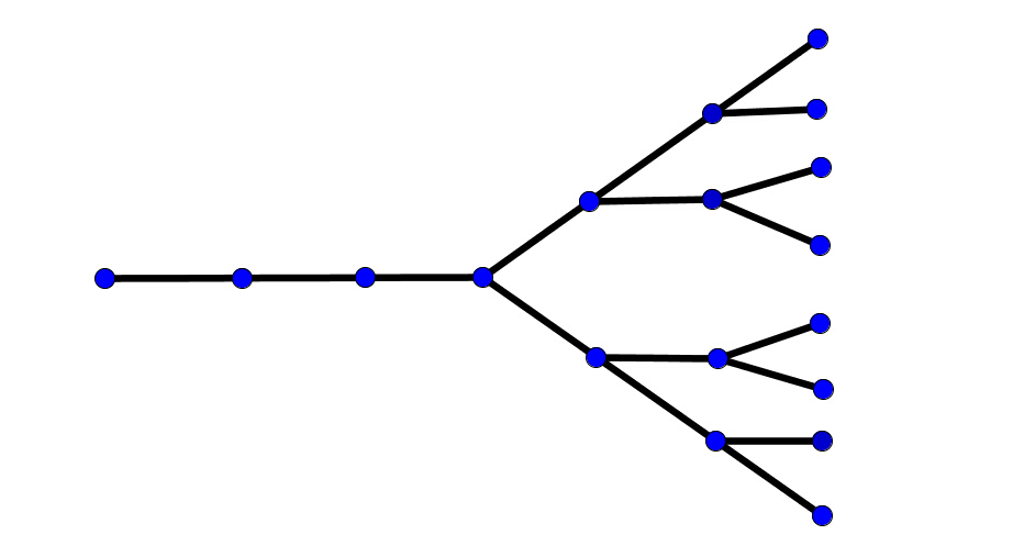
Figure 2. A tree with large doubling constant but limited maximal vertex degree.

The counting measure on an infinite graph is not necessarily a doubling measure. However, the counting measure on a finite graph is a doubling measure and its doubling constant could depend on the local topology and size of the graph, cf. the tree in Figure 2. In this paper, the graph ${\mathcal{G}}$ to describe our SDS is assumed to have its counting measure with the doubling property (2.1).

Assumption 1: The counting measure $\mu_{\mathcal{G}}$ of the graph ${\mathcal{G}}$ is a doubling measure,

(2.3) $$D_{0}({\mathcal{G}})<\infty.$$

Therefore the maximal vertex degree of graph $\mathcal{G}$ is finite,

$$\deg({\mathcal{G}})<\infty,$$

which could be understood as that there are limited direct communication channels for every agent in the SDS.

Definition 2.2.

The counting measure $\mu_{\mathcal{G}}$ is said to have polynomial growth if there exist positive constants $D_{1}({\mathcal{G}})$ and $d({\mathcal{G}})$ such that

(2.4) $$\mu_{\mathcal{G}}(B_{\mathcal{G}}(\lambda,r))\leq D_{1}({\mathcal{G}})(1+r)^{d({\mathcal{G}})}\ \ {\rm for\ all}\ \lambda\in G\ {\rm and}\ r\geq 0.$$

For the graph ${\mathcal{G}}$ associated with an SDS, we may consider minimal constants $d({\mathcal{G}})$ and $D_{1}({\mathcal{G}})$ in (2.4) as Beurling dimension and sampling density of the SDS respectively. We remark that

(2.5) $$d({\mathcal{G}})\geq 1,$$

because

$$\sup_{\lambda\in G}\mu_{\mathcal{G}}(B_{\mathcal{G}}(\lambda,r))\geq 1+r\ \ {\rm for\ all}\ 0\leq r\leq{\rm diam}({\mathcal{G}}),$$

where ${\rm diam}({\mathcal{G}}):=\sup_{\lambda,\lambda^{\prime}\in G}\rho_{\mathcal{G}}(\lambda,\lambda^{\prime})$ is the diameter of the graph ${\mathcal{G}}$.

Applying (2.1) repeatedly leads to the following general doubling property:

$$\mu_{\mathcal{G}}(B_{\mathcal{G}}(\lambda,sr))\leq(D_{0}({\mathcal{G}}))^{\lceil\log_{2}s\rceil}\mu_{\mathcal{G}}(B_{\mathcal{G}}(\lambda,r))\leq D_{0}({\mathcal{G}})s^{\log_{2}D_{0}({\mathcal{G}})}\mu_{\mathcal{G}}(B_{\mathcal{G}}(\lambda,r))$$

for all $\lambda\in G$, $s\geq 1$ and $r\geq 0$. Thus

$$\mu_{\mathcal{G}}(B_{\mathcal{G}}(\lambda,r))\leq D_{0}({\mathcal{G}})(1+r)^{\log_{2}D_{0}({\mathcal{G}})}\mu_{\mathcal{G}}\Big{(}B_{\mathcal{G}}\Big{(}\lambda,\frac{r}{1+r}\Big{)}\Big{)}=D_{0}({\mathcal{G}})(1+r)^{\log_{2}D_{0}({\mathcal{G}})},\ r\geq 0.$$

This shows that a doubling measure has polynomial growth.

Proposition 2.3.

If the counting measure $\mu_{\mathcal{G}}$ on a connected simple graph ${\mathcal{G}}$ is a doubling measure, then it has polynomial growth.

For a connected simple graph ${\mathcal{G}}$, its maximal vertex degree is finite if the counting measure $\mu_{\mathcal{G}}$ has polynomial growth, but the converse is not true. We observe that if the maximal vertex degree $\deg({\mathcal{G}})$ is finite, then the counting measure $\mu_{\mathcal{G}}$ has exponential growth,

(2.6) $$\mu_{\mathcal{G}}(B_{\mathcal{G}}(\lambda,r))\leq\frac{(\deg({\mathcal{G}}))^{r+1}-1}{\deg({\mathcal{G}})-1}\ \ {\rm for\ all}\ \lambda\in G\ {\rm and}\ r\geq 0.$$

2.3. Spatially distributed subsystems

For a connected simple graph ${\mathcal{G}}:=(G,S)$, take a maximal $N$-disjoint subset $G_{N}\subset G,0\leq N\in{\mathbb{R}}$, such that

(2.7) $$B_{\mathcal{G}}(\lambda,N)\mathbin{\scalebox{1.5}{$\cap$}}\big{(}\mathbin{\scalebox{1.5}{$\cup$}}_{\lambda_{m}\in G_{N}}B_{\mathcal{G}}(\lambda_{m},N)\big{)}\neq\emptyset\ \ {\rm for\ all}\ \lambda\in G,$$

and

(2.8) $$B_{\mathcal{G}}(\lambda_{m},N)\mathbin{\scalebox{1.5}{$\cap$}}B_{\mathcal{G}}(\lambda_{m^{\prime}},N)=\emptyset\ \ {\rm for\ all}\ \lambda_{m},\lambda_{m^{\prime}}\in G_{N}.$$

For $0\leq N<1$, it follows from (2.7) that $G_{N}=G$. For $N\geq 1$, there are many subsets $G_{N}$ of vertices satisfying (2.7) and (2.8). For instance, we can construct $G_{N}=\{\lambda_{m}\}_{m\geq 1}$ as follows: take a $\lambda_{1}\in G$ and define $\lambda_{m},\ m\geq 2$, recursively by

$$\lambda_{m}=\mathop{\operatorname*{argmin}}_{\lambda\in A_{m}}{\rho_{\mathcal{G}}(\lambda,\lambda_{1})},$$

where $A_{m}=\{\lambda\in G,\ B_{\mathcal{G}}(\lambda,N)\cap B_{\mathcal{G}}(\lambda_{m^{\prime}},N)=\emptyset,1\leq m^{\prime}\leq m-1\}$.

For a set $G_{N}$ satisfying (2.7) and (2.8), the family of balls $\{B_{\mathcal{G}}(\lambda_{m},N^{\prime}),\lambda_{m}\in G_{N}\}$ with $N^{\prime}\geq 2N$ provides a finite covering for $G$.

Proposition 2.4.

Let ${\mathcal{G}}:=(G,S)$ be a connected simple graph and $\mu_{\mathcal{G}}$ have the doubling property (2.3) with constant $D_{0}({\mathcal{G}})$. If $G_{N}$ satisfies (2.7) and (2.8), then

(2.9) $$1\leq\inf_{\lambda\in G}\Sigma_{\lambda_{m}\in G_{N}}\chi_{B_{\mathcal{G}}(\lambda_{m},N^{\prime})}(\lambda)\leq\sup_{\lambda\in G}\Sigma_{\lambda_{m}\in G_{N}}\chi_{B_{\mathcal{G}}(\lambda_{m},N^{\prime})}(\lambda)\leq(D_{0}({\mathcal{G}}))^{\lceil\log_{2}(2N^{\prime}/N+1)\rceil}$$

for all $N^{\prime}\geq 2N$.

For $N^{\prime}\geq 0$, define a family of spatially distributed subsystems

$${\mathcal{G}}_{\lambda,N^{\prime}}:=(B_{\mathcal{G}}(\lambda,N^{\prime}),S_{\lambda,N^{\prime}})$$

with fusion agents $\lambda\in G_{N}$, where $(\lambda^{\prime},\lambda^{\prime\prime})\in S_{\lambda,N^{\prime}}$ if $\lambda^{\prime},\lambda^{\prime\prime}\in B_{\mathcal{G}}(\lambda,N^{\prime})$ and $(\lambda^{\prime},\lambda^{\prime\prime})\in S$. Then the maximal $N$-disjoint property of the set $G_{N}$ means that the $N$-neighboring subsystems ${\mathcal{G}}_{\lambda_{m},N},\lambda_{m}\in G_{N}$, have no common agent. On the other hand, it follows from Proposition 2.4 that for any $N^{\prime}\geq 2N$, every agent in our SDS is in at least one and at most finitely many of the $N^{\prime}$-neighboring subsystems ${\mathcal{G}}_{\lambda_{m},N^{\prime}},\lambda_{m}\in G_{N}$. The above idea to split the SDS into subsystems of small sizes is crucial in our proposed distributed algorithm in Section 7 for stable signal reconstruction.

3. Signals on the graph $\mathcal{V}$

Let $V$ be the set of innovative positions of signals $f$ in (1.3), and ${\mathcal{G}=(G,S)}$ be the graph in (1.1) to represent our SDS. We build the graph ${\mathcal{H}}$ in (1.4) to describe our DSRS by associating every innovative position in $V$ with some anchor agents in $G$. In this paper, we consider DSRS with the following properties.

Assumption 2: There is a direct communication link between distinct anchor agents of an innovative position,

(3.1) $$(\lambda_{1},\lambda_{2})\in S\ {\rm if}\ (i,\lambda_{1})\ {\rm and}\ (i,\lambda_{2})\in T\ {\rm for\ some}\ i\in V.$$

Assumption 3: There are finitely many innovative positions for any anchor agent,

(3.2) $$L:=\sup_{\lambda\in G}\#\{i\in V,\ (i,\lambda)\in T\}<\infty.$$

Assumption 4: Any agent has an anchor agent within bounded distance,

(3.3) $$M:=\sup_{\lambda\in G}\inf\{\rho_{\mathcal{G}}(\lambda,\lambda^{\prime}),\ (i,\lambda^{\prime})\in T\ {\rm for\ some}\ i\in V\}<\infty.$$

The graph ${\mathcal{H}}$ associated with the above DSRS is a connected simple graph. Moreover, we have the following important properties about shortest paths between different vertices in ${\mathcal{H}}$.

Proposition 3.1.

Let the graph ${\mathcal{H}}$ in (1.4) satisfy (3.1). Then all intermediate vertices in the shortest paths in ${\mathcal{H}}$ to connect distinct vertices in ${\mathcal{H}}$ belong to the subgraph ${\mathcal{G}}$.

By Proposition 3.1,

(3.4) $$\rho_{\mathcal{H}}(\lambda,\lambda^{\prime})=\rho_{\mathcal{G}}(\lambda,\lambda^{\prime})\quad{\rm for\ all}\ \lambda,\lambda^{\prime}\in G,$$

and

(3.5) $$\rho_{\mathcal{H}}(i,i^{\prime})=2+\inf_{\lambda,\lambda^{\prime}\in G}\{\rho_{\mathcal{G}}(\lambda,\lambda^{\prime}):(i,\lambda),(i^{\prime},\lambda^{\prime})\in T\}\quad{\rm for\ all\ distinct}\ i,i^{\prime}\in V,$$

where $\rho_{\mathcal{H}}$ is the geodesic distance for the graph ${\mathcal{H}}$.

Let ${\mathcal{V}}$ be the graph in (1.6), where there is an edge between two distinct innovative positions if they share a common anchor agent. One may easily verify that the graph ${\mathcal{V}}$ is undirected and its maximal vertex degree is finite,

(3.6) $$\deg({\mathcal{V}})\leq L\sup_{i\in V}\#\{\lambda\in G,\ (i,\lambda)\in T\}\leq L(\deg({\mathcal{G}})+1)$$

by (2.2), (2.3), (3.1) and (3.2).

We cannot define a geodesic distance on ${\mathcal{V}}$ as in Subsection 2.1, since the graph ${\mathcal{V}}$ is unconnected in general. With the help of the graph ${\mathcal{H}}$ to describe our DSRS, we define a distance $\rho$ on the graph ${\mathcal{V}}$.

Proposition 3.2.

Let ${\mathcal{H}}$ be the graph in (1.4). Define a function $\rho:V\times V\longmapsto{\mathbb{R}}$ by

(3.7) $$\rho(i,i^{\prime})=\left\{\begin{array}[]{ll}0&{\rm if}\ i=i^{\prime}\\ \rho_{\mathcal{H}}(i,i^{\prime})-1&{\rm if}\ i\neq i^{\prime}.\end{array}\right.$$

If the graph $\mathcal{H}$ satisfies (3.1), then $\rho$ is a distance on the graph ${\mathcal{V}}$:

• $\rho(i,i^{\prime})\geq 0$ for all $i,i^{\prime}\in V$;

• $\rho(i,i^{\prime})=\rho(i^{\prime},i)$ for all $i,i^{\prime}\in V$;

• $\rho(i,i^{\prime})=0$ if and only if $i=i^{\prime}$; and

• $\rho(i,i^{\prime})\leq\rho(i,i^{\prime\prime})+\rho(i^{\prime\prime},i^{\prime})$ for all $i,i^{\prime},i^{\prime\prime}\in V$.

Clearly, the above distance between two endpoints of an edge in $\mathcal{V}$ is one. Denote the closed ball with center $i\in V$ and radius $r$ by

$$B(i,r)=\{i^{\prime}\in V,\ \rho(i,i^{\prime})\leq r\},$$

and the counting measure on $V$ by $\mu$. We say that $\mu$ is a doubling measure if

(3.8) $$\mu(B(i,2r))\leq D_{0}\mu(B(i,r))\ {\rm for\ all}\ i\in V\ {\rm and}\ r\geq 0,$$

and it has polynomial growth if

(3.9) $$\mu(B(i,r))\leq D_{1}(1+r)^{d}\ {\rm for\ all}\ i\in V\ {\rm and}\ r\geq 0,$$

where $D_{0}$, $D_{1}$ and $d$ are positive constants. The minimal constant $D_{0}$ for (3.8) to hold is known as the doubling constant, and the minimal constants $d$ and $D_{1}$ in (3.9) are called dimension and maximal rate of innovation for signals on the graph ${\mathcal{V}}$ respectively. The concept of rate of innovation was introduced in [72] and later extended in [61, 67]. The reader may refer to [10, 12, 29, 46, 50, 55, 59, 61, 67, 72] and references therein for sampling and reconstruction of signals with finite rate of innovation.

In the next two propositions, we show that the counting measure $\mu$ on ${\mathcal{V}}$ has the doubling property (respectively, the polynomial growth property) if and only if the counting measure $\mu_{\mathcal{G}}$ on ${\mathcal{G}}$ does.

Proposition 3.3.

Let ${\mathcal{G}}$ and ${\mathcal{H}}$ satisfy Assumptions 1 – 4. If $\mu_{\mathcal{G}}$ is a doubling measure with constant $D_{0}({\mathcal{G}})$, then

(3.10) $$\mu(B(i,2r))\leq L(D_{0}({\mathcal{G}}))^{2}\Big{(}\frac{(\deg({\mathcal{G}}))^{2M+3}-1}{\deg({\mathcal{G}})-1}\Big{)}\mu(B(i,r))\ \ {\rm for\ all}\ i\in V\ {\rm and}\ r\geq 0.$$

Conversely, if $\mu$ is a doubling measure with constant $D_{0}$, then

(3.11) $$\mu_{\mathcal{G}}(B_{\mathcal{G}}(\lambda,2r))\leq LD_{0}^{2}\Big{(}\frac{(\deg({\mathcal{G}}))^{2M+3}-1}{\deg({\mathcal{G}})-1}\Big{)}^{2}\mu_{\mathcal{G}}(B_{\mathcal{G}}(\lambda,r))\ \ {\rm for\ all}\ \lambda\in G\ {\rm and}\ r\geq 0.$$

Proposition 3.4.

Let ${\mathcal{G}}$ and ${\mathcal{H}}$ satisfy Assumptions 1 – 4. If $\mu_{\mathcal{G}}$ has polynomial growth with Beurling dimension $d({\mathcal{G}})$ and sampling density $D_{1}({\mathcal{G}})$, then

(3.12) $$\mu(B(i,r))\leq LD_{1}({\mathcal{G}})(1+r)^{d({\mathcal{G}})}\ \ {\rm for\ all}\ i\in V\ {\rm and}\ r\geq 0.$$

Conversely, if $\mu$ has polynomial growth with dimension $d$ and maximal rate of innovation $D_{1}$, then

(3.13) $$\mu_{\mathcal{G}}(B_{\mathcal{G}}(\lambda,r))\leq 2^{d}\Big{(}\frac{(\deg({\mathcal{G}}))^{2M+3}-1}{\deg({\mathcal{G}})-1}\Big{)}D_{1}(1+r)^{d}\ \ {\rm for\ all}\ \lambda\in G\ {\rm and}\ r\geq 0.$$

By (2.5), Propositions 3.3 and 3.4, we conclude that signals in (1.3) have their dimension $d$ being the same as the Beurling dimension $d({\mathcal{G}})$, and their maximal rate $D_{1}$ of innovation being approximately proportional to the sampling density $D_{1}({\mathcal{G}})$.

Theorem 3.5.

Let ${\mathcal{G}}$ and ${\mathcal{H}}$ satisfy Assumptions 1 – 4. Then

(3.14) $$d({\mathcal{G}})=d\geq 1$$

and

(3.15) $$L^{-1}D_{1}\leq D_{1}({\mathcal{G}})\leq 2^{d}\Big{(}\frac{(\deg({\mathcal{G}}))^{2M+3}-1}{\deg({\mathcal{G}})-1}\Big{)}D_{1}.$$

We finish this section with a remark about signals on our graph $\mathcal{V}$, cf. [52, 53, 56].

Remark 3.6.

Signals on the graph ${\mathcal{V}}$ are analog in nature, while signals on graphs in most of the literature are discrete ([52, 53, 56]). Let ${\bf p}_{\lambda}$ and ${\bf p}_{i}$ be the physical positions of the agent $\lambda\in G$ and innovative position $i\in V$, respectively. If there exist positive constants $A$ and $B$ such that

$$A\sum_{i\in V}|c(i)|^{2}\leq\sum_{i\in V}|f({\bf p}_{i})|^{2}+\sum_{\lambda\in G}|f({\bf p}_{\lambda})|^{2}\leq B\sum_{i\in V}|c(i)|^{2}$$

for all signals $f$ with the parametric representation (1.3), then we can establish a one-to-one correspondence between the analog signal $f$ and the discrete signal $F$ on the graph ${\mathcal{H}}$, where

$$F(u)=f({\bf p}_{u}),\ u\in G\cup V.$$

The above family of discrete signals $F$ forms a linear space, which could be a Paley-Wiener space associated with some positive-semidefinite operator (such as Laplacian) on the graph ${\mathcal{H}}$. Using the above correspondence, our theory for signal sampling and reconstruction applies by assuming that the impulse response $\psi_{\lambda}$ of every agent $\lambda\in G$ is supported on ${\bf p}_{u},u\in G\cup V$.

4. Sensing matrices with polynomial off-diagonal decay

Let ${\mathcal{H}}$ be the connected simple graph in (1.4) to describe our DSRS, and the sensing matrix ${\bf S}$ associated with the DSRS be as in (1.7). As agents in the DSRS have limited sensing ability, we assume in this paper that the sensing matrix ${\bf S}$ in (1.7) satisfies

(4.1) $${\bf S}\in{\mathcal{J}}_{\alpha}({\mathcal{G}},{\mathcal{V}})\ {\rm for\ some}\ \alpha>d,$$

where

(4.2) $${\mathcal{J}}_{\alpha}({\mathcal{G}},{\mathcal{V}}):=\big{\{}{\bf A}:=(a(\lambda,i))_{\lambda\in G,i\in V},\ \|{\bf A}\|_{{\mathcal{J}}_{\alpha}({\mathcal{G}},{\mathcal{V}})}<\infty\big{\}}$$

is the Jaffard class ${\mathcal{J}}_{\alpha}({\mathcal{G}},{\mathcal{V}})$ of matrices with polynomial off-diagonal decay, and

(4.3) $$\|{\bf A}\|_{{\mathcal{J}}_{\alpha}({\mathcal{G}},{\mathcal{V}})}:=\sup_{\lambda\in G,i\in V}(1+\rho_{\mathcal{H}}(\lambda,i))^{\alpha}|a(\lambda,i)|,\quad\alpha\geq 0.$$

The reader may refer to [37, 38, 40, 58, 60, 65] for matrices with various off-diagonal decay.

We observe that a matrix in ${\mathcal{J}}_{\alpha}({\mathcal{G}},{\mathcal{V}}),\alpha>d$, defines a bounded operator from $\ell^{p}(V)$ to $\ell^{p}(G),1\leq p\leq\infty$.

Proposition 4.1.

Let ${\mathcal{G}}$ and ${\mathcal{H}}$ satisfy Assumptions 1 – 4, ${\mathcal{V}}$ be as in (1.6), and let $\mu_{\mathcal{G}}$ have polynomial growth with Beurling dimension $d$ and sampling density $D_{1}({\mathcal{G}})$. If ${\mathbf{A}}\in{\mathcal{J}}_{\alpha}({\mathcal{G}},{\mathcal{V}})$ for some $\alpha>d$, then

(4.4) $$\|{\mathbf{A}}{\mathbf{c}}\|_{p}\leq\frac{D_{1}({\mathcal{G}})L\alpha}{\alpha-d}\|{\mathbf{A}}\|_{{\mathcal{J}}_{\alpha}({\mathcal{G}},{\mathcal{V}})}\|{\bf c}\|_{p}\ \ {\rm for\ all}\ {\mathbf{c}}\in\ell^{p},1\leq p\leq\infty.$$

For a DSRS with its sensing matrix in ${\mathcal{J}}_{\alpha}({\mathcal{G}},{\mathcal{V}})$, we obtain from (1.10) and Proposition 4.1 that a signal with bounded amplitude vector generates a bounded sampling data vector.

Define band matrix approximations of a matrix ${\mathbf{A}}=(a(\lambda,i))_{\lambda\in G,i\in V}$ by

(4.5) $${\mathbf{A}}_{s}:=(a_{s}(\lambda,i))_{\lambda\in G,i\in V},\ s\geq 0,$$

where

$$a_{s}(\lambda,i)=\left\{\begin{array}[]{ll}a(\lambda,i)&{\rm if}\ \ \rho_{\mathcal{H}}(\lambda,i)\leq s\\ 0&{\rm if}\ \ \rho_{\mathcal{H}}(\lambda,i)>s.\end{array}\right.$$

We say a matrix $\mathbf{A}$ has bandwidth $s$ if $\mathbf{A}=\mathbf{A}_{s}$. Clearly, any matrix $\mathbf{A}$ with bounded entries and bandwidth $s$ belongs to Jaffard class ${\mathcal{J}}_{\alpha}({\mathcal{G}},{\mathcal{V}})$,

$$\|{\bf A}\|_{{\mathcal{J}}_{\alpha}({\mathcal{G}},{\mathcal{V}})}\leq(s+1)^{\alpha}\|{\bf A}\|_{{\mathcal{J}}_{0}({\mathcal{G}},{\mathcal{V}})}\ {\rm\ for\ all\ }\alpha\geq 0.$$

In our DSRS, the sensing matrix $\mathbf{S}$ has bandwidth $s$ means that any agent can only detect signals at innovative positions within their geodesic distance less than or equal to $s$. In the next proposition, we show that matrices in the Jaffard class can be well approximated by band matrices.

Proposition 4.2.

Let graphs ${\mathcal{G}}$, ${\mathcal{H}}$, ${\mathcal{V}}$, $d$ and $D_{1}({\mathcal{G}})$ be as in Proposition 4.1. If ${\mathbf{A}}\in{\mathcal{J}}_{\alpha}({\mathcal{G}},{\mathcal{V}})$ for some $\alpha>d$, then

(4.6) $$\|({\mathbf{A}}-{\mathbf{A}}_{s}){\mathbf{c}}\|_{p}\leq\frac{D_{1}({\mathcal{G}})L\alpha}{\alpha-d}(s+1)^{-\alpha+d}\|{\mathbf{A}}\|_{{\mathcal{J}}_{\alpha}({\mathcal{G}},{\mathcal{V}})}\|{\mathbf{c}}\|_{p}\ \ {\rm for\ all}\ {\bf c}\in\ell^{p},1\leq p\leq\infty,$$

where ${\mathbf{A}}_{s},s\geq 1$, are band matrices in (4.5).

The above band matrix approximation property will be used later in the establishment of a local stability criterion in Section 6 and exponential convergence of a distributed reconstruction algorithm in Section 7.

5. Robustness of distributed sampling and reconstruction systems

Let ${\bf S}$ be the sensing matrix associated with our DSRS. We say that a reconstruction algorithm $\Delta$ is a perfect reconstruction in noiseless environment if

(5.1) $$\Delta({\bf S}{\bf c})={\bf c}\ \ {\rm for\ all}\ {\bf c}\in\ell^{\infty}.$$

In this section, we first study robustness of the DSRS in term of the $\ell^{\infty}$-stability.

Proposition 5.1.

Let ${\mathcal{G}}$ and ${\mathcal{H}}$ satisfy Assumptions 1 – 4, ${\mathcal{V}}$ be as in (1.6), $\mu_{\mathcal{G}}$ have polynomial growth with Beurling dimension $d$, and let $\mathbf{S}$ satisfy (4.1). Then there is a reconstruction algorithm $\Delta$ with the suboptimal approximation property (1.12) and the perfect reconstruction property (5.1) if and only if ${\bf S}$ has $\ell^{\infty}$-stability.

The sufficiency in Proposition 5.1 holds by taking $\Delta=\Delta_{\infty}$ in (1.13), while the necessity follows by applying (1.12) to $\boldsymbol{\eta}={\bf S}{\bf d}$ with ${\bf d}\in\ell^{\infty}$.

The $\ell^{\infty}$-stability of a matrix can not be verified in a distributed manner, up to our knowledge. In the next theorem, we circumvent such a verification problem by reducing $\ell^{\infty}$-stability of a matrix in Jaffard class to its $\ell^{2}$-stability, for which a distributed verifiable criterion will be provided in Section 6.

Theorem 5.2.

Let ${\mathcal{G}},{\mathcal{H}},{\mathcal{V}}$ and $d$ be as in Proposition 5.1, and let ${\mathbf{A}}\in{\mathcal{J}}_{\alpha}({\mathcal{G}},{\mathcal{V}})$ for some $\alpha>d$. If ${\mathbf{A}}$ has $\ell^{2}$-stability, then it has $\ell^{p}$-stability for all $1\leq p\leq\infty$.

The reader may refer to [3, 54, 65] for equivalence of $\ell^{p}$-stability of localized matrices for different $1\leq p\leq\infty$. The lower and upper $\ell^{p}$-stability bounds of the matrix ${\bf A}$ depend on its $\ell^{2}$-stability bounds and local features of the graph ${\mathcal{H}}$. From the proof of Theorem 5.2, we observe that they depend only on the $\ell^{2}$-stability bounds, ${\mathcal{J}}_{\alpha}({\mathcal{G}},{\mathcal{V}})$-norm of the matrix ${\mathbf{A}}$, maximal vertex degree ${\rm deg}({\mathcal{G}})$, the Beurling dimension $d$, the sampling density $D_{1}({\mathcal{G}})$, and the constants $L$ and $M$ in (3.2) and (3.3). So the sensing matrix of our DSRS may have its $\ell^{p}$-stability bounds independent of the size of the DSRS.

For the graph ${\mathcal{V}}$ in (1.6) and the distance $\rho$ in (3.7), define

(5.2) $${\mathcal{J}}_{\alpha}({\mathcal{V}}):=\big{\{}{\bf A}:=(a(i,i^{\prime}))_{i,i^{\prime}\in V},\ \|{\bf A}\|_{{\mathcal{J}}_{\alpha}({\mathcal{V}})}<\infty\big{\}},$$

where

(5.3) $$\|{\bf A}\|_{{\mathcal{J}}_{\alpha}({\mathcal{V}})}:=\sup_{i,i^{\prime}\in V}(1+\rho(i,i^{\prime}))^{\alpha}|a(i,i^{\prime})|,\ \alpha\geq 0.$$

The proof of Theorem 5.2 depends highly on the following Wiener’s lemma for the matrix algebra ${\mathcal{J}}_{\alpha}({\mathcal{V}}),\alpha>d$.

Theorem 5.3.

Let ${\mathcal{V}}$ be as in (1.6) and its counting measure $\mu$ satisfy (3.9). If ${\mathbf{A}}\in{\mathcal{J}}_{\alpha}({\mathcal{V}}),\alpha>d$, and ${\bf A}^{-1}$ is bounded on $\ell^{2}$, then ${\mathbf{A}}^{-1}\in{\mathcal{J}}_{\alpha}({\mathcal{V}})$ too.

Wiener’s lemma has been established for infinite matrices, pseudodifferential operators, and integral operators satisfying various off-diagonal decay conditions ([11, 33, 35, 37, 38, 40, 58, 60, 62, 65]). It has been shown to be crucial for well-localization of dual Gabor/wavelet frames, fast implementation in numerical analysis, local reconstruction in sampling theory, local features of spatially distributed optimization, etc. The reader may refer to the survey papers [36, 43] for historical remarks, motivation and recent advances.

The Wiener’s lemma (Theorem 5.3) is also used to establish the sub-optimal approximation property (1.12) for the “least squares” solution $\Delta_{2}({\bf z})$ in (1.15), for which a distributed algorithm is proposed in Section 7.

Theorem 5.4.

Let ${\mathcal{G}},{\mathcal{H}}$ and ${\mathcal{V}}$ be as in Proposition 5.1. Assume that the sensing matrix ${\mathbf{S}}$ satisfies (4.1) and it has $\ell^{2}$-stability. Then there exists a positive constant $C$ such that

(5.4) $$\|\Delta_{2}({\bf z})-{\bf c}\|_{\infty}\leq C\|\boldsymbol{\eta}\|_{\infty}\quad{\rm for\ all}\ {\bf c},{\boldsymbol{\eta}}\in\ell^{\infty},$$

where ${\bf z}={\bf S}{\bf c}+\boldsymbol{\eta}$.

6. Stability criterion for distributed sampling and reconstruction system

Let ${\mathcal{H}}$ be the connected simple graph in (1.4) to describe our DSRS. Given $\lambda^{\prime}\in G$ and a positive integer $N$, define truncation operators $\chi_{\lambda^{\prime},G}^{N}$ and $\chi_{\lambda^{\prime},V}^{N}$ by

$$\chi_{\lambda^{\prime},G}^{N}:\ \ell^{p}(G)\ni(d(\lambda))_{\lambda\in G}\longmapsto\big{(}d(\lambda)\chi_{B_{\mathcal{H}}(\lambda^{\prime},N)\cap G}(\lambda)\big{)}_{\lambda\in G}\in\ell^{p}(G)$$

and

$$\chi_{\lambda^{\prime},V}^{N}:\ \ell^{p}(V)\ni(c(i))_{i\in V}\longmapsto\big{(}c(i)\chi_{B_{\mathcal{H}}(\lambda^{\prime},N)\cap V}(i)\big{)}_{i\in V}\in\ell^{p}(V),$$

where $1\leq p\leq\infty$ and

$$B_{\mathcal{H}}(u,r):=\{v\in G\cup V,\ \rho_{\mathcal{H}}(u,v)\leq r\}$$

is the closed ball in ${\mathcal{H}}$ with center $u\in{\mathcal{H}}$ and radius $r\geq 0$.

For any matrix ${\mathbf{A}}\in{\mathcal{J}}_{\alpha}({\mathcal{G}},{\mathcal{V}})$ with $\ell^{2}$-stability, we observe that its quasi-main submatrices $\chi_{\lambda}^{2N}{\mathbf{A}}\chi_{\lambda}^{N},\lambda\in G$, of size $O(N^{d})$ have uniform $\ell^{2}$-stability for large $N$.

Theorem 6.1.

Let ${\mathcal{G}}$ and ${\mathcal{H}}$ satisfy Assumptions 1 – 4, ${\mathcal{V}}$ be as in (1.6), $\mu_{\mathcal{G}}$ have polynomial growth with Beurling dimension $d$ and sampling density $D_{1}({\mathcal{G}})$, and let ${\mathbf{A}}\in{\mathcal{J}}_{\alpha}({\mathcal{G}},{\mathcal{V}})$ for some $\alpha>d$. If ${\mathbf{A}}$ has $\ell^{2}$-stability with lower bound $A\|{\mathbf{A}}\|_{{\mathcal{J}}_{\alpha}({\mathcal{G}},{\mathcal{V}})}$, then

(6.1) $$\|\chi_{\lambda,G}^{2N}{\mathbf{A}}\chi_{\lambda,V}^{N}{\bf c}\|_{2}\geq\frac{A}{2}\|{\mathbf{A}}\|_{{\mathcal{J}}_{\alpha}({\mathcal{G}},{\mathcal{V}})}\|\chi_{\lambda,V}^{N}{\bf c}\|_{2},\ {\bf c}\in\ell^{2}$$

for all $\lambda\in G$ and all integers $N$ satisfying

(6.2) $$2D_{1}({\mathcal{G}})N^{-\alpha+d}\sqrt{L\alpha/(\alpha-d)}\leq A.$$

The above theorem provides a guideline to design a distributed algorithm for signal reconstruction, see Section 7. Surprisingly, the converse of Theorem 6.1 is true, cf. the stability criterion in [64, Theorem 2.1] for convolution-dominated matrices.

Theorem 6.2.

Let ${\mathcal{G}},{\mathcal{H}},{\mathcal{V}}$ be as in Theorem 6.1, and ${\mathbf{A}}\in{\mathcal{J}}_{\alpha}({\mathcal{G}},{\mathcal{V}})$ for some $\alpha>d$. If there exist a positive constant $A_{0}$ and an integer $N_{0}\geq 3$ such that

(6.3) $$\hskip-14.45377ptA_{0}\geq 4(D_{0}({\mathcal{G}}))^{2}D_{1}({\mathcal{G}})LN_{0}^{-\min(\alpha-d,1)}\times\left\{\begin{array}[]{ll}\Big{(}\frac{4\alpha}{3(\alpha-d)}+\frac{2(\alpha-1)(\alpha-d)}{\alpha-d-1}\Big{)}&\hskip-7.22743pt{\rm if}\ \alpha>d+1\\ \big{(}\frac{10(d+1)}{3}+2d\ln N_{0}\big{)}&\hskip-7.22743pt{\rm if}\ \alpha=d+1\\ \Big{(}\frac{4\alpha}{3(\alpha-d)}+\frac{4d}{d+1-\alpha}\Big{)}&\hskip-7.22743pt{\rm if}\ \alpha<d+1,\end{array}\right.$$

and for all $\lambda\in G$,

(6.4) $$\|\chi_{\lambda,G}^{2N_{0}}{\mathbf{A}}\chi_{\lambda,V}^{N_{0}}{\bf c}\|_{2}\geq A_{0}\|{\mathbf{A}}\|_{{\mathcal{J}}_{\alpha}({\mathcal{G}},{\mathcal{V}})}\|\chi_{\lambda,V}^{N_{0}}{\bf c}\|_{2},\ {\bf c}\in\ell^{2},$$

then ${\mathbf{A}}$ has $\ell^{2}$-stability,

(6.5) $$\|{\bf A}{\bf c}\|_{2}\geq\frac{A_{0}\|{\mathbf{A}}\|_{{\mathcal{J}}_{\alpha}({\mathcal{G}},{\mathcal{V}})}}{12(D_{0}({\mathcal{G}}))^{2}}\|{\bf c}\|_{2},\ {\bf c}\in\ell^{2}.$$

Observe that the right hand side of (6.3) could be arbitrarily small when $N_{0}$ is sufficiently large. This together with Theorem 6.1 implies that the requirements (6.3) and (6.4) are necessary for the $\ell^{2}$-stability property of any matrix in ${\mathcal{J}}_{\alpha}({\mathcal{G}},{\mathcal{V}})$. As shown in the example below, the term $N_{0}^{-\min(\alpha-d,1)}$ in (6.3) cannot be replaced by $N_{0}^{-\beta}$ with high order $\beta>1$ even if the matrix ${\bf A}$ has finite bandwidth.

Example 6.3.

Let ${\bf A}_{0}=(a_{0}(i-j))_{i,j\in{\mathbb{Z}}}$ be the bi-infinite Toeplitz matrix with symbol $\sum_{k\in{\mathbb{Z}}}a_{0}(k)e^{-ik\xi}=1-e^{-i\xi}$. Then ${\bf A}_{0}$ belongs to the Jaffard class ${\mathcal{J}}_{\alpha}({\mathbb{Z}},{\mathbb{Z}})$ for all $\alpha\geq 0$ and it does not have $\ell^{2}$-stability. On the other hand, for any $\lambda\in G=V={\mathbb{Z}}$ and $N_{0}\geq 1$,

$$\inf_{\|\chi_{\lambda,V}^{N_{0}}{\bf c}\|_{2}=1}\|\chi_{\lambda,G}^{2N_{0}}{\mathbf{A}}_{0}\chi_{\lambda,V}^{N_{0}}{\bf c}\|_{2}=\inf_{\|\chi_{\lambda,V}^{N_{0}}{\bf c}\|_{2}=1}\|{\mathbf{A}}_{0}\chi_{\lambda,V}^{N_{0}}{\bf c}\|_{2}$$

$$= \inf_{|d_{1}|^{2}+\cdots+|d_{2N_{0}+1}|^{2}=1}\sqrt{|d_{1}|^{2}+|d_{1}-d_{2}|^{2}+\cdots+|d_{2N_{0}}-d_{2N_{0}+1}|^{2}+|d_{2N_{0}+1}|^{2}}$$

$$= 2\sin\frac{\pi}{4N_{0}+4}\geq\frac{1}{2}N_{0}^{-1},$$

where the last equality follows from [41, Lemma 1 of Chapter 9].

For our DSRS with sensing matrix ${\bf S}$ having the polynomial off-diagonal decay property (4.1), the uniform stability property (6.4) could be verified by finding minimal eigenvalues of its quasi-main submatrices $\chi_{\lambda,V}^{N_{0}}{\mathbf{S}}^{T}\chi_{\lambda,G}^{2N_{0}}{\mathbf{S}}\chi_{\lambda,V}^{N_{0}},\lambda\in G$, of size about $O(N_{0}^{d})$. The above verification could be implemented on agents in the DSRS via its computing and communication abilities. This provides a practical tool to verify $\ell^{2}$-stability of a DSRS and to design a robust (dynamic) DSRS against supplement, replacement and impairment of agents.

7. Exponential convergence of a distributed reconstruction algorithm

In our DSRS, agents could essentially catch signals not far from their locations. So one may expect that a signal near any innovative position should substantially be determined by sampling data of neighboring agents, while data from distant agents should have (almost) no influence in the reconstruction. The most desirable method to meet the above expectation is local exact reconstruction, which could be implemented in a distributed manner without iterations ([6, 39, 63, 68]). In such a linear reconstruction procedure, there is a left-inverse $\mathbf{T}$ of the sensing matrix ${\bf S}$ with finite bandwidth,

$${\bf T}{\bf S}={\bf I}.$$

For our DSRS, such a left-inverse $\mathbf{T}$ with finite bandwidth may not exist and/or it is difficult to find even it exists. We observe that

$${\mathbf{S}}^{\dagger}:=({\mathbf{S}}^{T}{\mathbf{S}})^{-1}{\mathbf{S}}^{T}$$

is a left-inverse well approximated by matrices with finite bandwidth, and

(7.1) $${\bf d}_{2}={\mathbf{S}}^{\dagger}{\bf z}$$

is a suboptimal approximation, where ${\bf z}$ is given in (1.11). However, it is infeasible to find the pseudo-inverse ${\mathbf{S}}^{\dagger}$, because the DSRS does not have a central processor and it has huge amounts of agents and large number of innovative positions. In this section, we introduce a distributed algorithm to find the suboptimal approximation ${\bf d}_{2}$ in (7.1).

Let ${\mathcal{H}}$ be the connected simple graph in (1.4) to describe our DSRS, and the sensing matrix ${\mathbf{S}}\in{\mathcal{J}}_{\alpha}({\mathcal{G}},{\mathcal{V}}),\alpha>d$, have $\ell^{2}$-stability. Then ${\bf d}_{2}$ in (7.1) is the unique solution to the “normal” equation

(7.2) $${\mathbf{S}}^{T}{\mathbf{S}}{\bf d}_{2}={\bf S}^{T}{\bf z}.$$

As principal submatrices $\chi_{\lambda,V}^{N}{\mathbf{S}}^{T}{\mathbf{S}}\chi_{\lambda,V}^{N}$ of the positive definite matrix ${\bf S}^{T}{\bf S}$ are uniformly stable, we solve localized linear systems

(7.3) $$\chi_{\lambda,V}^{N}{\mathbf{S}}^{T}{\mathbf{S}}\chi_{\lambda,V}^{N}{\bf d}_{\lambda,N}=\chi_{\lambda,V}^{N}{\bf S}^{T}{\bf z},\ \lambda\in G,$$

of size $O(N^{d})$, whose solutions ${\bf d}_{\lambda,N}$ are supported in the ball $B_{\mathcal{H}}(\lambda,N)\cap V$. One of crucial results of this paper is that for large integer $N$, the solution ${\bf d}_{\lambda,N}$ provides a reasonable approximation of the “least squares” solution ${\bf d}_{2}$ inside the half ball $B_{\mathcal{H}}(\lambda,N/2)\cap V$, see (7.6) in Proposition 7.1. However, the above local approximation can not be implemented distributedly in the DSRS, as only agents on the graph ${\mathcal{G}}$ have computing and telecommunication ability. So we propose to compute

(7.4) $${\bf w}_{\lambda,N}:=\chi_{\lambda,G}^{N}{\bf S}\chi_{\lambda,V}^{N}(\chi_{\lambda,V}^{N}{\mathbf{S}}^{T}{\mathbf{S}}\chi_{\lambda,V}^{N})^{-1}{\bf d}_{\lambda,N}=\chi_{\lambda,G}^{N}{\bf S}\chi_{\lambda,V}^{N}(\chi_{\lambda,V}^{N}{\mathbf{S}}^{T}{\mathbf{S}}\chi_{\lambda,V}^{N})^{-2}\chi_{\lambda,V}^{N}{\bf S}^{T}{\bf z}$$

instead, which approximates

(7.5) $${\bf w}_{LS}:={\bf S}({\bf S}^{T}{\bf S})^{-1}{\bf d}_{2}$$

inside $B_{\mathcal{G}}(\lambda,N/2)\cap G$, see (7.7) in the proposition below.

Proposition 7.1.

Let ${\mathcal{G}}$ and ${\mathcal{H}}$ satisfy Assumptions 1 – 4, ${\mathcal{V}}$ be as in (1.6), and let the sensing matrix ${\mathbf{S}}\in{\mathcal{J}}_{\alpha}({\mathcal{G}},{\mathcal{V}}),\alpha>d$, have $\ell^{2}$-stability with lower stability bound $A\|{\bf S}\|_{{\mathcal{J}}_{\alpha}({\mathcal{G}},{\mathcal{V}})}$. Take an integer $N$ satisfying (6.2), and set

$$\theta=\frac{2\alpha-2d}{2\alpha-d}\in(0,1)\ \ {\rm and}\ \ r_{0}=1-\frac{A^{2}(\alpha-d)^{2}}{2^{\alpha+1}D_{1}D_{1}(\mathcal{G})\alpha^{2}}.$$

Then

(7.6) $$\hskip-1.4457pt\|\chi_{\lambda,V}^{N/2}({\bf d}_{\lambda,N}-{\bf d}_{2})\|_{\infty}\leq D_{3}(N+1)^{-\alpha+d}\|{\bf d}_{2}\|_{\infty}$$

and

(7.7) $$\hskip-1.4457pt\|\chi_{\lambda,G}^{N/2}({\bf w}_{\lambda,N}-{\bf w}_{LS})\|_{\infty}\leq D_{4}(N+1)^{-\alpha+d}\|{\bf d}_{2}\|_{\infty},$$

where $D_{3}=\frac{2^{2\alpha-d+1}\alpha D_{1}D_{2}}{\alpha-d}$, $D_{4}=\big{(}\frac{2^{3\alpha-d+3}\alpha L^{2}D_{1}(\mathcal{G})D_{2}^{2}}{\alpha-d}+LD_{2}\big{)}\|\mathbf{S}\|_{\mathcal{J}_{\alpha}(\mathcal{G},\mathcal{V})}^{-1}$, and

(7.8) $$D_{2}=\sum\limits_{n=0}^{\infty}\Big{(}\frac{2^{2\alpha+d/2+4}D_{1}^{3}\alpha^{2}}{r_{0}^{1-\theta}(\alpha-d)^{2}}\Big{)}^{\frac{2-\theta}{(1-\theta)^{2}}n^{\log_{2}^{(2-\theta)}}}r_{0}^{n}.$$

Take a maximal $\frac{N}{4}$-disjoint subset $G_{N/4}\subset G$ satisfying (2.7) and (2.8). We patch ${\bf w}_{\lambda,N},\lambda\in G_{N/4}$, in (7.4) together to generate a linear approximation

(7.9) $${\bf w}_{N}^{*}=\sum_{\lambda\in G_{N/4}}{\boldsymbol{\Theta}}_{\lambda,N}\chi_{\lambda,G}^{N/2}{\bf w}_{\lambda,N}$$

of the bounded vector ${\bf w}_{LS}$, where ${\boldsymbol{\Theta}}_{\lambda,N}$ is a diagonal matrix with diagonal entries

$${\theta}_{\lambda,N}(\lambda^{\prime\prime})=\frac{\chi_{B_{\mathcal{G}}(\lambda,N/2)}(\lambda^{\prime\prime})}{\sum_{\lambda^{\prime}\in G_{N/4}}\chi_{B_{\mathcal{G}}(\lambda^{\prime},N/2)}(\lambda^{\prime\prime})},\ \lambda^{\prime\prime}\in G.$$

The above approximation is well-defined as $\{B_{\mathcal{G}}(\lambda^{\prime},N/2),\ \lambda^{\prime}\in G_{N/4}\}$ is a finite covering of $G$ by (3.4) and Proposition 2.4. Moreover, we obtain from Proposition 7.1 that

(7.10) $$\|{\bf w}^{*}_{N}-{\bf w}_{LS}\|_{\infty} \hskip-5.78172pt= \hskip-5.78172pt\Big{\|}\sum_{\lambda\in G_{N/4}}{\boldsymbol{\Theta}}_{\lambda,N}\chi_{\lambda,G}^{N/2}({\bf w}_{\lambda,N}-{\bf w}_{LS})\Big{\|}_{\infty}$$

$$\hskip-5.78172pt\leq \hskip-5.78172pt\sup_{\lambda^{\prime\prime}\in G}\sum_{\lambda\in G_{N/4}}\theta_{\lambda,N}(\lambda^{\prime\prime})\|\chi_{\lambda,G}^{N/2}({\bf w}_{\lambda,N}-{\bf w}_{LS})\|_{\infty}$$

$$\hskip-5.78172pt\leq \hskip-5.78172ptD_{4}(N+1)^{-\alpha+d}\|{\bf d}_{2}\|_{\infty}.$$

Therefore, the moving consensus ${\bf w}^{*}_{N}$ of ${\bf w}_{\lambda,N},\lambda\in G_{N/4}$, provides a good approximation to ${\bf w}_{LS}$ in (7.5) for large $N$. In addition, ${\bf w}^{*}_{N}$ depends on the observation ${\bf z}$ linearly,

(7.11) $${\bf w}_{N}^{*}={\bf R}_{N}{\bf S}^{T}{\bf z}$$

for some matrix ${\bf R}_{N}$ with bandwidth $2N$ and

(7.12) $$\|{\bf R}_{N}\|_{{\mathcal{J}}_{\alpha}({\mathcal{G}},{\mathcal{V}})}\leq D_{5}:=\frac{(\alpha-d)^{2}LD_{2}^{2}}{\alpha^{2}D_{1}D_{1}(\mathcal{G})\|\mathbf{S}\|_{{\mathcal{J}}_{\alpha}({\mathcal{G}},{\mathcal{V}})}^{3}}.$$

Given noisy samples ${\bf z}$, we may use ${\bf w}_{N}^{*}$ in (7.11) as the first approximation of ${\bf w}_{LS}$,

(7.13) $${\bf w}_{1}={\bf R}_{N}{\bf S}^{T}{\bf z}$$

and recursively define

(7.14) $${\bf w}_{n+1}={\bf w}_{n}+{\bf w}_{1}-{\bf R}_{N}{\bf S}^{T}{\bf S}{\bf S}^{T}{\bf w}_{n},\ n\geq 1.$$

In the next theorem, we show that the above sequence ${\bf w}_{n},n\geq 1$, converges exponentially to some bounded vector ${\bf w}$, not necessarily ${\bf w}_{LS}$, satisfying the consistent condition

(7.15) $${\bf S}^{T}{\bf w}={\bf S}^{T}{\bf w}_{LS}={\bf d}_{2}.$$

Theorem 7.2.

Let ${\mathcal{G}},{\mathcal{H}}$ and ${\mathcal{V}}$ be as in Proposition 7.1, and let ${\bf w}_{n},n\geq 1$, be as in (7.13) and (7.14). Suppose that $N$ satisfies (6.2) and

(7.16) $$r_{1}:=\frac{D_{1}(\mathcal{G})D_{4}L\alpha}{\alpha-d}\|{\bf S}\|_{{\mathcal{J}}_{\alpha}(\mathcal{G},\mathcal{V})}(N+1)^{-\alpha+d}<1.$$

Set

$$D_{6}=\frac{2^{2\alpha+2}\alpha L^{3}(D_{1}(\mathcal{G}))^{2}D_{2}^{2}}{(\alpha-d)(1-r_{1})D_{1}\|{\bf S}\|_{{\mathcal{J}}_{\alpha}(\mathcal{G},\mathcal{V})}}.$$

Then ${\bf w}_{n}$ and ${\bf S}^{T}{\bf w}_{n},n\geq 1$, converge exponentially to a bounded vector ${\bf w}$ in (7.15) and the “least squares” solution ${\bf d}_{2}$ in (7.1) respectively,

(7.17) $$\|{\bf w}_{n}-{\bf w}\|_{\infty}\leq D_{6}r_{1}^{n}\|{\bf d}_{2}\|_{\infty}$$

and

(7.18) $$\|{\bf S}^{T}{\bf w}_{n}-{\bf d}_{2}\|_{\infty}\leq\frac{D_{1}(\mathcal{G})D_{6}L\alpha}{\alpha-d}\|\mathbf{S}\|_{{\mathcal{J}}_{\alpha}({\mathcal{G}},{\mathcal{V}})}r_{1}^{n}\|{\bf d}_{2}\|_{\infty},\ n\geq 1.$$

By the above theorem, each agent should have minimal storage, computing, and telecommunication capabilities. Furthermore, the algorithm (7.13) and (7.14) will have faster convergence (hence less delay for signal reconstruction) by selecting large $N$ when agents have larger storage, more computing power, and higher telecommunication capabilities. In addition, no iteration is needed for sufficiently large $N$, and the reconstructed signal is approximately to the one obtained by the finite-section method, cf. [20] and simulations in Section 8.

The iterative algorithm (7.13) and (7.14) can be recast as follows:

(7.19) $${\bf w}_{1}={\bf R}_{N}{\bf S}^{T}{\bf z}\ \ {\rm and}\ \ {\bf e}_{1}={\bf w}_{1}-{\bf R}_{N}{\bf S}^{T}{\bf S}{\bf S}^{T}{\bf w}_{1},$$

and

(7.20) $$\left\{\begin{array}[]{l}{\bf w}_{n+1}={\bf w}_{n}+{\bf e}_{n}\\ {\bf e}_{n+1}={\bf e}_{n}-{\bf R}_{N}{\bf S}^{T}{\bf S}{\bf S}^{T}{\bf e}_{n},\ n\geq 1.\end{array}\right.$$

Next, we present a distributed implementation of the algorithm (7.19) and (7.20) when ${\bf S}$ has bandwidth $s$. Select a threshold $\epsilon$ and an integer $N\geq s$ satisfying (7.16). Write

$$\left\{\begin{array}[]{l}{\bf S}^{T}=({\bf a}(i,\lambda))_{i\in V,\lambda\in G}\\ {\bf R}_{N}{\bf S}^{T}=({\bf b}_{N}(\lambda,\lambda^{\prime}))_{\lambda,\lambda^{\prime}\in G}\\ {\bf R}_{N}{\bf S}^{T}{\bf S}{\bf S}^{T}=({\bf c}_{N}(\lambda,\lambda^{\prime}))_{\lambda,\lambda^{\prime}\in G}\\ {\bf z}=({\bf z}(\lambda))_{\lambda\in G},\end{array}\right.$$

and

$${\bf w}_{n}=({\bf w}_{n}(\lambda))_{\lambda\in G}\ \ {\rm and}\ \ {\bf e}_{n}=({\bf e}_{n}(\lambda))_{\lambda\in G},\ n\geq 1.$$

We assume that any agent $\lambda\in G$ stores vectors ${\bf a}(i,\lambda^{\prime}),{\bf b}_{N}(\lambda,\lambda^{\prime}),{\bf c}_{N}(\lambda,\lambda^{\prime})$ and ${\bf z}(\lambda^{\prime})$, where $(i,\lambda)\in T$ and $\lambda^{\prime}\in B_{\mathcal{G}}(\lambda,2N+3s)$. The following is the distributed implementation of the algorithm (7.19) and (7.20) for an agent $\lambda\in G$.

Distributed algorithm (7.19) and (7.20) for signal reconstruction:

• Input ${\bf a}(i,\lambda^{\prime}),{\bf b}_{N}(\lambda,\lambda^{\prime}),{\bf c}_{N}(\lambda,\lambda^{\prime})$ and ${\bf z}(\lambda^{\prime})$, where $(i,\lambda)\in T$ and $\lambda^{\prime}\in B_{\mathcal{G}}(\lambda,2N+3s)$.

• Input stop criterion $\epsilon>0$ and maximal number of iteration steps $K$.

• Compute ${\bf w}(\lambda)=\sum_{\lambda^{\prime}\in B_{\mathcal{G}}(\lambda,2N+s)}{\bf b}_{N}(\lambda,\lambda^{\prime}){\bf z}(\lambda^{\prime})$.

• Communicate with neighboring agents in $B_{\mathcal{G}}(\lambda,2N+3s)$ to obtain data ${\bf w}(\lambda^{\prime})$, $\lambda^{\prime}\in B_{\mathcal{G}}(\lambda,2N+3s)$.

• Evaluate the sampling error term ${\bf e}(\lambda)={\bf w}(\lambda)-\sum_{\lambda^{\prime}\in B_{\mathcal{G}}(\lambda,2N+3s)}{\bf c}_{N}(\lambda,\lambda^{\prime}){\bf w}(\lambda^{\prime})$.

• Communicate with neighboring agents in $B_{\mathcal{G}}(\lambda,2N+3s)$ to obtain error data ${\bf e}(\lambda^{\prime})$, $\lambda^{\prime}\in B_{\mathcal{G}}(\lambda,2N+3s)$.

• for $n=2$ to $K$ do

  • Compute $\delta=\max_{\lambda^{\prime}\in B_{\mathcal{G}}(\lambda,2N+3s)}|{\bf e}(\lambda^{\prime})|$.

  • Stop if $\delta\leq\epsilon$, else do

  • Update ${\bf w}(\lambda)={\bf w}(\lambda)+{\bf e}(\lambda)$.

  • Update ${\bf e}(\lambda)={\bf e}(\lambda)-\sum_{\lambda^{\prime}\in B_{\mathcal{G}}(\lambda,2N+3s)}{\bf c}_{N}(\lambda,\lambda^{\prime}){\bf e}(\lambda^{\prime})$.

  • Communicate with neighboring agents located in $B_{\mathcal{G}}(\lambda,2N+3s)$ to obtain error data ${\bf e}(\lambda^{\prime})$, $\lambda^{\prime}\in B_{\mathcal{G}}(\lambda,2N+3s)$.

• end for

We conclude this section by discussing the complexity of the distributed algorithm (7.19) and (7.20), which depends essentially on $N$. In its implementation, the data storage requirement for each agent is about $(L+3)(2N+3s+1)^{d}$. In each iteration, the computational cost for each agent is about $O(N^{d})$ mainly used for updating the error ${\bf e}$. The communication cost for each agent is about $O(N^{d+\beta})$ if the communication between distant agents $\lambda,\lambda^{\prime}\in G$, processed through their shortest path, has its cost being proportional to $(\rho_{\mathcal{G}}(\lambda,\lambda^{\prime}))^{\beta}$ for some $\beta\geq 1$. By Theorem 7.2, the number of iteration steps needed to reach the accuracy $\epsilon$ is about $O(\ln(1/\epsilon)/\ln N)$. Therefore the total computational and communication cost for each agent are about $O(\ln(1/\epsilon)N^{d}/\ln N)$ and $O(\ln(1/\epsilon)N^{d+\beta}/\ln N)$, respectively.

8. Numerical simulations

In this section, we present two simulations to demonstrate the distributed algorithm (7.19) and (7.20) for stable signal reconstruction.

Agents in the first simulation are almost uniformly deployed on the circle of radius $R/5$, and their locations are at

$$\lambda_{l}:=\frac{R}{5}\Big{(}\cos\frac{2\pi\theta_{l}}{R},\sin\frac{2\pi\theta_{l}}{R}\Big{)},\ 1\leq l\leq R,$$

where $R\geq 1$ and $\theta_{l}\in l+[-1/4,1/4]$ are randomly selected. Every agent in the SDS has a direct communication channel to its two adjacent agents. Then the graph ${\mathcal{G}}_{c}=(G_{c},S_{c})$ to describe the SDS is a cycle graph, where $G_{c}=\{\lambda_{1},\ldots,\lambda_{R}\}$ and $S_{c}=\big{\{}(\lambda_{1},\lambda_{2}),\ldots,(\lambda_{R-1},\lambda_{R})$, $(\lambda_{R},\lambda_{1})$, $(\lambda_{1},\lambda_{R})$, $(\lambda_{R},\lambda_{R-1}),\ldots,(\lambda_{2},\lambda_{1})\big{\}}$. Take innovative positions

$${\bf p}_{i}:=r_{i}\Big{(}\cos\frac{2\pi i}{R},\ \sin\frac{2\pi i}{R}\Big{)},\ 1\leq i\leq R,$$

deployed almost uniformly near the circle of radius $R/5$, where $r_{i}\in R/5+[-1/4,1/4]$ are randomly selected. Given any innovative position ${\bf p}_{i},1\leq i\leq R$, it has three anchor agents $\lambda_{i},\lambda_{i-1}$ and $\lambda_{i+1}$, where $\lambda_{0}=\lambda_{R}$ and $\lambda_{R+1}=\lambda_{1}$. Set $V_{c}=\{{\bf p}_{i},1\leq i\leq R\}$ and $T_{c}=\{({\bf p}_{i},\lambda_{i-j}),i=1,\ldots,R\ {\rm and}\ j=0,\pm 1\}$. Then ${\mathcal{H}}_{c}=(G_{c}\cap V_{c},S_{c}\cup T_{c}\cup T_{c}^{*})$ is the graph to describe the DSRS, see Figure 3.

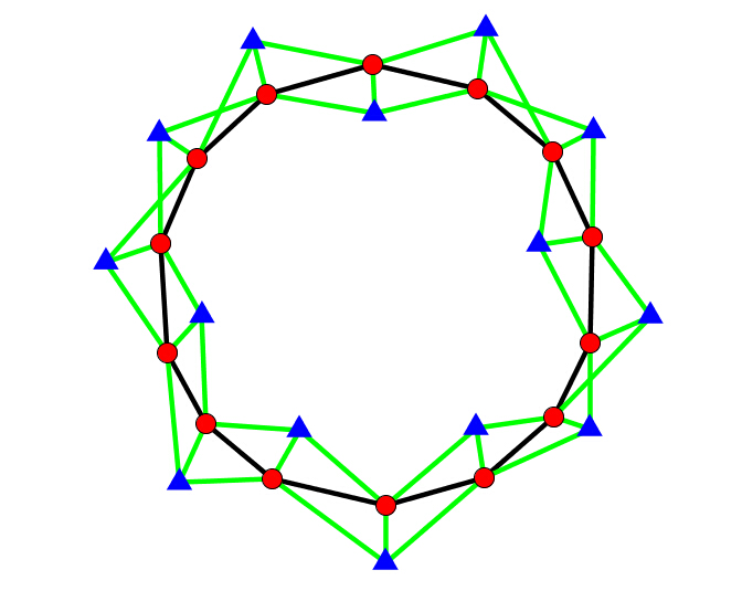
Figure 3. The graph ${\mathcal{H}}_{c}=(G_{c}\cap V_{c},S_{c}\cup T_{c}\cup T_{c}^{*})$ to describe the DSRS in the first simulation, where vertices in $G_{c}$, edges in $S_{c}$, vertices in $V_{c}$ and edges in $T_{c}\cup T_{c}^{\ast}$ are plotted in red circles, black lines, blue triangles and green lines, respectively.

Let $\varphi({\bf t}):=\exp(-(t_{1}^{2}+t_{2}^{2})/2)$ for ${\bf t}=(t_{1},t_{2})$. Gaussian signals

(8.1) $$f({\bf t})=\sum_{i=1}^{R}c(i)\varphi({\bf t}-{\bf p}_{i})$$

to be sampled and reconstructed have their amplitudes $c(i)\in[0,1]$ being randomly chosen, see the left image of Figure 4.

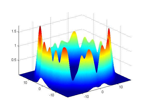
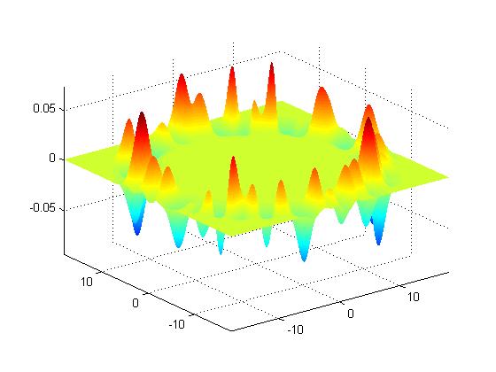
Figure 4. Plotted on the left is the signal $f$ in (8.1) with $R=80$. On the right is the difference between the signal $f$ and the reconstructed signal $f_{n,N,\delta}$ with $n=10,N=6$ and $\delta=0.05$.

In the first simulation, we consider ideal sampling procedure. Thus for the agent $\lambda_{l},1\leq l\leq R$, the noisy sampling data acquired is

(8.2) $$y_{\delta}(l)=\sum_{i=1}^{R}c(i)\varphi(\lambda_{l}-{\bf p}_{i})+\eta(l),$$

where $\eta(l)\in[-\delta,\delta]$ are randomly generated with bounded noise level $\delta>0$.

Our first simulation shows that the distributed algorithm (7.19) and (7.20) converges for $N\geq 5$ and the convergence rate is almost independent of the network size $R$, cf. the upper bound estimate in (7.18).

Let $f_{n,N,\delta}({\bf t}):=\sum_{i=1}^{R}c_{n,N,\delta}(i)\varphi({\bf t}-{\bf p}_{i})$ be the reconstructed signal in the $n$-th iteration by applying the distributed algorithm (7.19) and (7.20) from the noisy sampling data in (8.2), see the right image of Figure 4. Define maximal reconstruction errors

$$\epsilon(n,N,\delta):=\left\{\begin{array}[]{ll}\max_{1\leq i\leq R}|c(i)|&{\rm if}\ n=0,\\ \max_{1\leq i\leq R}|c_{n,N,\delta}(i)-c(i)|&{\rm if}\ n\geq 1.\end{array}\right.$$

Presented in Table 1 is the average of reconstruction errors $\epsilon(n,N,\delta)$ with 500 trials in noiseless environment ($\delta=0$), where the network size $R$ is 80. It indicates that the proposed distributed algorithm (7.19) and (7.20) has faster convergence rate for larger $N\geq 5$, and we only need three iteration steps to have a near perfect reconstruction from its noiseless samples when $N=10$.

Table 1. Maximal reconstruction errors $\epsilon(n,N,\delta)$ with $\delta=0$

	5	6	7	8	9	10
0	0.9874	0.9881	0.9878	0.9876	0.9877	0.9884
1	0.9875	0.4463	0.3073	0.1940	0.1055	0.0523
2	0.6626	0.2046	0.0794	0.0271	0.0124	0.0024
3	0.3624	0.0926	0.0240	0.0045	0.0014	0.0001
4	0.2535	0.0443	0.0068	0.0006	0.0001	0.0000
5	0.1742	0.0206	0.0018	0.0001	0.0000	0.0000
6	0.1169	0.0093	0.0005	0.0000	0.0000	0.0000
7	0.0840	0.0042	0.0001	0.0000	0.0000	0.0000
8	0.0579	0.0017	0.0000	0.0000	0.0000	0.0000
9	0.0411	0.0007	0.0000	0.0000	0.0000	0.0000
10	0.0289	0.0003	0.0000	0.0000	0.0000	0.0000

The robustness of the proposed algorithm (7.19) and (7.20) against sampling noises is tested and confirmed, see Figure 4. Moreover, it is observed that the maximal reconstruction error $\epsilon(n,N,\delta)$ with large $n$ depends almost linearly on the noise level $\delta$, cf. the sub-optimal approximation property in Theorem 5.4.

In the next simulation, agents are uniformly deployed on two concentric circles and each agent has direct communication channels to its three adjacent agents. Then the graph ${\mathcal{G}}_{p}=(G_{p},S_{p})$ to describe our SDS is a prism graph with vertices having physical locations,

$$\mu_{l}:=\left\{\begin{array}[]{ll}\frac{R}{10}\big{(}\cos\frac{4\pi\theta_{l}}{R},\sin\frac{4\pi\theta_{l}}{R}\big{)}&\ {\rm if}\ \ 1\leq l\leq\frac{R}{2}\\ \big{(}\frac{R}{10}+1\big{)}\big{(}\cos\frac{4\pi\theta_{l}}{R},\sin\frac{4\pi\theta_{l}}{R}\big{)}&\ {\rm if}\ \ \frac{R}{2}+1\leq l\leq R,\end{array}\right.$$

where $R\geq 2$ and $\theta_{l}\in l+[-1/4,1/4],1\leq l\leq R$, are randomly selected. The innovative positions

$${\bf q}_{i}:=r_{i}\big{(}\cos\frac{4\pi i}{R},\ \sin\frac{4\pi i}{R}\big{)},\ 1\leq i\leq\frac{R}{2},$$

have four anchor agents $\mu_{i},\mu_{i+1}$, $\mu_{i+R/2}$ and $\mu_{i+R/2+1}$, where $\mu_{0}=\mu_{R/2}$, $\mu_{R+1}=\mu_{R/2+1}$, and $r_{i}\in\frac{R}{10}+[\frac{1}{4},\frac{3}{4}]$ are randomly selected. Set $V_{p}=\{{\bf q}_{i},1\leq i\leq\frac{R}{2}\}$ and $T_{p}=\{({\bf q}_{i},\mu_{i+j}),i=1,\ldots,\frac{R}{2}\ {\rm and}\ j=0,1,\frac{R}{2},\frac{R}{2}+1\}$. Thus the graph ${\mathcal{H}}_{p}=(G_{p}\cap V_{p},S_{p}\cup T_{p}\cup T_{p}^{*})$ to describe our DSRS is a connected simple graph, see the left image of Figure 5.

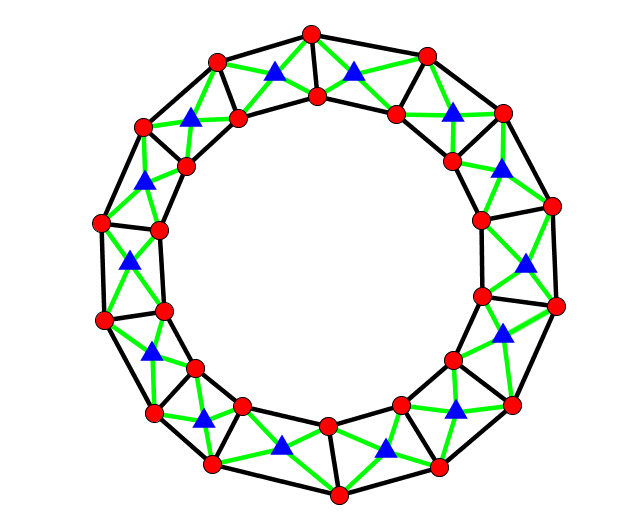
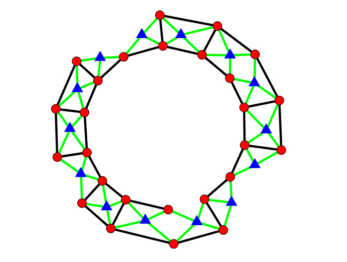
Figure 5. Plotted on the left is the graph ${\mathcal{H}}_{p}=(G_{p}\cap V_{p},S_{p}\cup T_{p}\cup T_{p}^{*})$ to describe the DSRS, where vertices in $G_{p}$ and $V_{p}$ are in red circles and blue triangles, and edges in $S_{p}$ and $T_{p}\cup T_{p}^{\ast}$ are in black solid lines and green solid lines, respectively. On the right is a subgraph of ${\mathcal{H}}_{p}$, where some agents are completely dysfunctional and some have communication channels to one or two of their nearby agents clogged.

Following the first simulation, we consider the ideal sampling procedure of signals,

(8.3) $$g({\bf t})=\sum_{i=1}^{R/2}d(i)\varphi({\bf t}-{\bf q}_{i}),$$

where $d(i)\in[0,1],1\leq i\leq R/2$, are randomly selected, see the left image of Figure 6.

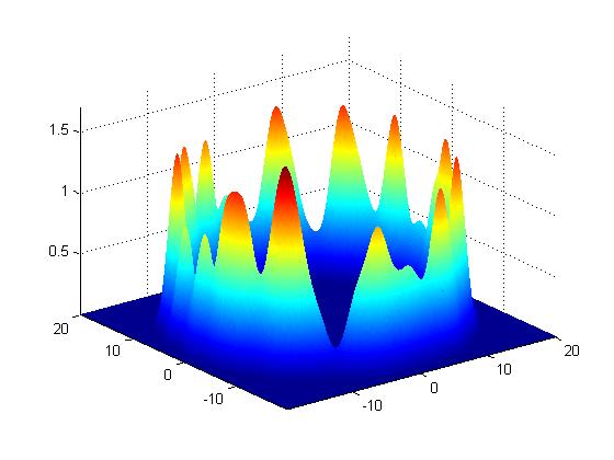
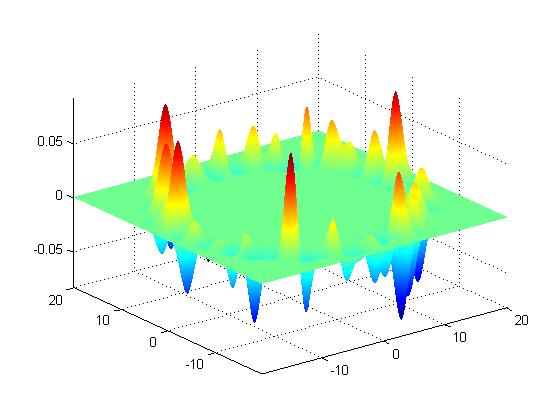
Figure 6. Plotted on the left is the signal $g$ in (8.3) with $R=160$. On the right is the difference between the signal $g$ and its approximation $g_{n,N,\delta}$, where $n=4,N=6,\delta=0.05$, and agents located at $\mu_{1},\mu_{87}$ are completely dysfunctional, while agents located at $\mu_{11},\mu_{51},\mu_{91}$ have their partial communication channels clogged.

Then the noisy sampling data acquired by the agent $\mu_{l},1\leq l\leq R$, is

(8.4) $$y_{\delta}(l)=\sum_{i=1}^{R/2}d(i)\varphi(\mu_{l}-{\bf q}_{i})+\eta(l),$$

where $\eta(l)\in[-\delta,\delta]$ are randomly selected with bounded noise level $\delta>0$. Applying the distributed algorithm (7.19) and (7.20), we obtain approximations

(8.5) $$g_{n,N,\delta}({\bf t})=\sum_{i=1}^{R/2}d_{n,N,\delta}(i)\varphi({\bf t}-{\bf q}_{i}),\ n\geq 1,$$

of the signal $g$ in (8.3). Our simulations illustrate that the distributed algorithm (7.19) and (7.20) converges for $N\geq 3$ and the signal $g$ can be reconstructed near perfectly from its noiseless samples in 12 steps for $N=3$, 7 steps for $N=4$, 5 steps for $N=5$, 4 steps for $N=6$, and 3 steps for $N=7$, cf. Table 1 in the first simulation.

The robustness of the proposed distributed algorithm (7.19) and (7.20) against sampling noises and dysfunctions of agents in the DSRS is tested and confirmed, see the right graph of Figure 5 and the right image of Figure 6.

9. Proofs

In this section, we include proofs of Propositions 2.4, 3.1, 3.2, 3.3, 3.4, 4.1, 4.2, 7.1, and Theorems 5.2, 5.3, 5.4, 6.1, 6.2, 7.2.

9.1. Proof of Proposition 2.4

For any $\lambda\in G$, take $\lambda_{m}\in G_{N}$ with $B_{\mathcal{G}}(\lambda,N)\cap B_{\mathcal{G}}(\lambda_{m},N)\neq\emptyset$. Then

$$\rho_{\mathcal{G}}(\lambda,\lambda_{m})\leq\rho_{\mathcal{G}}(\lambda,\lambda^{\prime})+\rho_{\mathcal{G}}(\lambda^{\prime},\lambda_{m})\leq 2N,$$

where $\lambda^{\prime}$ is a vertex in $B_{\mathcal{G}}(\lambda,N)\cap B_{\mathcal{G}}(\lambda_{m},N)$. This proves that for any $N^{\prime}\geq 2N$, balls $\{B_{\mathcal{G}}(\lambda_{m},N^{\prime}),\lambda_{m}\in G_{N}\}$ provide a covering for $G$,

(9.1) $$G\subset\bigcup_{\lambda_{m}\in G_{N}}B_{\mathcal{G}}(\lambda_{m},N^{\prime}),$$

and hence the first inequality in (2.9) follows.

Now we prove the last inequality in (2.9). Take $\lambda\in G$. For any $\lambda_{m},\lambda_{m^{\prime}}\in G_{N}\cap B_{\mathcal{G}}(\lambda,N^{\prime})$,

$$\rho_{\mathcal{G}}(\lambda^{\prime},\lambda_{m^{\prime}})\leq\rho_{\mathcal{G}}(\lambda^{\prime},\lambda_{m})+\rho_{\mathcal{G}}(\lambda_{m},\lambda)+\rho_{\mathcal{G}}(\lambda,\lambda_{m^{\prime}})\leq 2N^{\prime}+N$$

for all $\lambda^{\prime}\in B(\lambda_{m},N)$, which implies that

(9.2) $$B_{\mathcal{G}}(\lambda_{m},N)\subset B_{\mathcal{G}}(\lambda_{m^{\prime}},2N^{\prime}+N).$$

Hence

(9.3) $$\sum_{\lambda_{m}\in G_{N}}\chi_{B_{\mathcal{G}}(\lambda_{m},N^{\prime})}(\lambda)\hskip-7.22743pt \leq\hskip-7.22743pt \frac{\mu_{\mathcal{G}}(\cup_{\lambda_{m}\in G_{N}\cap B_{\mathcal{G}}(\lambda,N^{\prime})}B_{\mathcal{G}}(\lambda_{m},N))}{\inf_{\lambda_{m}\in G_{N}\cap B_{\mathcal{G}}(\lambda,N^{\prime})}\mu_{\mathcal{G}}(B_{\mathcal{G}}(\lambda_{m},N))}$$

$$\leq\hskip-7.22743pt \sup_{\lambda_{m}\in G_{N}\cap B_{\mathcal{G}}(\lambda,N^{\prime})}\frac{\mu_{\mathcal{G}}(B_{\mathcal{G}}(\lambda_{m},2N^{\prime}+N))}{\mu_{\mathcal{G}}(B_{\mathcal{G}}(\lambda_{m},N))}\leq(D_{0}({\mathcal{G}}))^{\lceil\log_{2}(2N^{\prime}/N+1)\rceil},$$

where the first inequality holds as $B_{\mathcal{G}}(\lambda_{m},N),\lambda_{m}\in V_{N}$, are disjoint, the second one is true by (9.2), and the third inequality follows from the doubling assumption (2.1).

9.2. Proof of Proposition 3.1

By the structure of the graph ${\mathcal{H}}$, it suffices to show that the shortest path in ${\mathcal{H}}$ to connect distinct vertices $\lambda,\lambda^{\prime}\in G$ must be a path in its subgraph ${\mathcal{G}}$. Suppose on the contrary that $\lambda u_{1}\cdots u_{k-1}u_{k}u_{k+1}\cdots u_{n}\lambda^{\prime}$ is a shortest path in ${\mathcal{H}}$ of length $\rho_{\mathcal{H}}(\lambda,\lambda^{\prime})$ with vertex $u_{k}$ along the path belonging to $V$. Then $u_{k-1}$ and $u_{k+1}$ are anchor agents of $u_{k}$ in $G$.

For the case that $u_{k-1}$ and $u_{k+1}$ are distinct anchor agents of the innovative position $u_{k}$, $(u_{k-1},u_{k+1})\in S$ by (3.1). Hence $\lambda u_{1}\cdots u_{k-1}u_{k+1}\cdots u_{n}\lambda^{\prime}$ is a path of length $\rho_{\mathcal{H}}(\lambda,\lambda^{\prime})-1$ to connect vertices $\lambda$ and $\lambda^{\prime}$, which is a contradiction.

Similarly for the case that $u_{k-1}$ and $u_{k+1}$ are the same, $\lambda u_{1}\cdots u_{k-1}u_{k+2}\cdots u_{n}\lambda^{\prime}$ is a path of length $\rho_{\mathcal{H}}(\lambda,\lambda^{\prime})-2$ to connect vertices $\lambda$ and $\lambda^{\prime}$. This is a contradiction.

9.3. Proof of Proposition 3.2

The non-negativity and symmetry is obvious, while the identity of indiscernibles holds since there is no edge assigned in ${\mathcal{H}}$ between two distinct vertices in $V$.

Now we prove the triangle inequality

(9.4) $$\rho(i,i^{\prime})\leq\rho(i,i^{\prime\prime})+\rho(i^{\prime\prime},i^{\prime})\ \ {\rm for\ distinct\ vertices}\ i,i^{\prime},i^{\prime\prime}\in V.$$

Let $m=\rho(i,i^{\prime\prime})$ and $n=\rho(i^{\prime\prime},i^{\prime})$. Take a path $iv_{1}\ldots v_{m}i^{\prime\prime}$ of length $m+1$ to connect $i$ and $i^{\prime\prime}$, and another path $i^{\prime\prime}u_{1}\ldots u_{n}i^{\prime}$ of length $n+1$ to connect $i^{\prime\prime}$ and $i^{\prime}$. If $v_{m}=u_{1}$, then $iv_{1}\ldots v_{m}u_{2}\cdots u_{n}i^{\prime}$ is a path of length $m+n$ to connect vertices $i$ and $i^{\prime}$, which implies that

(9.5) $$\rho(i,i^{\prime})\leq m+n-1<\rho(i,i^{\prime\prime})+\rho(i^{\prime\prime},i^{\prime}).$$

If $v_{m}\neq u_{1}$, then $(v_{m},u_{1})$ is an edge in the graph ${\mathcal{G}}$ (and then also in the graph ${\mathcal{H}}$) by (3.1). Thus $iv_{1}\ldots v_{m}u_{1}u_{2}\cdots u_{n}i^{\prime}$ is a path of length $m+n+1$ to connect vertices $i$ and $i^{\prime}$, and

(9.6) $$\rho(i,i^{\prime})\leq m+n=\rho(i,i^{\prime\prime})+\rho(i^{\prime\prime},i^{\prime}).$$

Combining (9.5) and (9.6) proves (9.4).

9.4. Proof of Proposition 3.3

To prove Proposition 3.3, we need two lemmas comparing measures of balls in graphs ${\mathcal{G}}$ and ${\mathcal{V}}$.

Lemma 9.1.

If ${\mathcal{H}}$ satisfies (3.1) and (3.2), then

(9.7) $$\mu(B(i,r))\leq L\mu_{\mathcal{G}}(B_{\mathcal{G}}(\lambda,r))\ \ {\rm for\ any}\ \lambda\in G\ {\rm with}\ (i,\lambda)\in T.$$

Proof.

Let $i^{\prime}\in B(i,r)$ with $i^{\prime}\neq i$. By Proposition 3.1, there exists a path $\lambda_{1}\ldots\lambda_{n}$ of length $\rho(i,i^{\prime})-1$ in the graph ${\mathcal{G}}$ such that $(i,\lambda_{1}),(i^{\prime},\lambda_{n})\in T$. Then

$$\rho_{\mathcal{G}}(\lambda,\lambda_{n})\leq\rho_{\mathcal{G}}(\lambda,\lambda_{1})+\rho_{\mathcal{G}}(\lambda_{1},\lambda_{n})\leq\rho(i,i^{\prime})\leq r$$

as either $\lambda_{1}=\lambda$ or $(\lambda,\lambda_{1})$ is an edge in ${\mathcal{G}}$ by (3.1). This shows that for any innovative position $i^{\prime}\in B(i,r)$ there exists an anchor agent $\lambda_{n}$ in the ball $B_{\mathcal{G}}(\lambda,r)$. This observation together with (3.2) proves (9.7). ∎

Lemma 9.2.

If ${\mathcal{H}}$ satisfies (2.3), (3.1) and (3.3), then

(9.8) $$\mu_{\mathcal{G}}(B_{\mathcal{G}}(\lambda,r))\leq\Big{(}\sup_{\lambda^{\prime}\in G}\mu_{\mathcal{G}}(B_{\mathcal{G}}(\lambda^{\prime},2M+2))\Big{)}\mu(B(i,r+M+1))$$

for any $\lambda\in G$ and $r\geq M+1$, where $(i,\lambda^{\prime})\in T$ and $\lambda^{\prime}\in B_{\mathcal{G}}(\lambda,M)$.

Proof.

Let $\lambda_{1}=\lambda$ and take $\Lambda=\{\lambda_{m}\}_{m\geq 1}$ such that (i) $B_{\mathcal{G}}(\lambda_{m},M+1)\subset B_{\mathcal{G}}(\lambda,r)$ for all $\lambda_{m}\in\Lambda$; (ii) $B_{\mathcal{G}}(\lambda_{m},M+1)\bigcap B_{\mathcal{G}}(\lambda_{m^{\prime}},M+1)=\emptyset$ for all distinct vertices $\lambda_{m},\lambda_{m^{\prime}}\in\Lambda$; and (iii) $B_{\mathcal{G}}(\tilde{\lambda},M+1)\bigcap\big{(}\bigcup_{\lambda_{m}\in\Lambda}B_{\mathcal{G}}(\lambda_{m},M+1)\big{)}\neq\emptyset$ for all $\tilde{\lambda}\in B_{\mathcal{G}}(\lambda,r)$. The set $\Lambda$ could be considered as a maximal $(M+1)$-disjoint subset of $B_{\mathcal{G}}(\lambda,r)$. Following the argument used in the proof of Proposition 2.4, $\{B_{\mathcal{G}}(\lambda_{m},2(M+1))\}_{\lambda_{m}\in\Lambda}$ forms a covering of the ball $B(\lambda,r)$, which implies that

(9.9) $$\hskip-7.22743pt\mu_{\mathcal{G}}(B_{\mathcal{G}}(\lambda,r))\leq\Big{(}\sup_{\lambda_{m}\in\Lambda}\mu_{\mathcal{G}}(B_{\mathcal{G}}(\lambda_{m},2M+2))\Big{)}\#\Lambda\leq\Big{(}\sup_{\lambda^{\prime}\in G}\mu_{\mathcal{G}}(B_{\mathcal{G}}(\lambda^{\prime},2M+2))\Big{)}\#\Lambda.$$

For $\lambda_{m}\in\Lambda$, define

$$V_{\lambda_{m}}=\{i^{\prime}\in V,(i^{\prime},\tilde{\lambda})\in T\ {\rm for\ some}\ \tilde{\lambda}\in B_{\mathcal{G}}(\lambda_{m},M)\}.$$

Then it follows from (3.3) that

(9.10) $$\#V_{\lambda_{m}}\geq 1\ {\rm for\ all}\ \lambda_{m}\in\Lambda.$$

Observe that the distance of anchor agents associated with innovative positions in distinct $V_{\lambda_{m}}$ is at least 2 by the second requirement (ii) for the set $\Lambda$. This together with the assumption (3.1) implies that

(9.11) $$V_{\lambda_{m}}\cap V_{\lambda_{m^{\prime}}}=\emptyset\ \ {\rm for\ distinct}\ \lambda_{m},\lambda_{m^{\prime}}\in\Lambda.$$

Combining (9.9), (9.10) and (9.11) leads to

(9.12) $$\mu_{\mathcal{G}}(B_{\mathcal{G}}(\lambda,r))\leq\Big{(}\sup_{\lambda^{\prime}\in G}\mu_{\mathcal{G}}(B_{\mathcal{G}}(\lambda^{\prime},2M+2))\Big{)}\#\Big{(}\cup_{\lambda_{m}\in\Lambda}V_{\lambda_{m}}\Big{)}.$$

Take $i\in V$ with $(i,\lambda^{\prime})\in T$ for some $\lambda^{\prime}\in B_{\mathcal{G}}(\lambda,M)$, and $i^{\prime}\in V_{\lambda_{m}},\lambda_{m}\in\Lambda$. Then

$$\rho_{\mathcal{H}}(i,\lambda)\leq\rho_{\mathcal{H}}(i,\lambda^{\prime})+\rho_{\mathcal{H}}(\lambda^{\prime},\lambda)\leq M+1,$$

and

$$\rho_{\mathcal{H}}(i^{\prime},\lambda)\leq\rho_{\mathcal{H}}(i^{\prime},\tilde{\lambda})+\rho_{\mathcal{H}}(\tilde{\lambda},\lambda)\leq r+1,$$

where $\tilde{\lambda}\in B_{\mathcal{G}}(\lambda_{m},M)$ and $(i^{\prime},\tilde{\lambda})\in T$. Thus

(9.13) $$\rho(i,i^{\prime})\leq r+M+1.$$

Then the desired estimate (9.8) follows from (9.12) and (9.13). ∎

We are ready to prove Proposition 3.3.

Proof of Proposition 3.3.

First we prove the doubling property (3.10) for the measure $\mu$. Take $i\in V$. Then for $r\geq 2(M+1)$ it follows from Lemmas 9.1 and 9.2 that

(9.14) $$\hskip-5.78172pt\mu(B(i,2r)) \hskip-5.78172pt\leq \hskip-5.78172ptL\mu_{\mathcal{G}}(B_{\mathcal{G}}(\lambda,2r))\leq L(D_{0}({\mathcal{G}}))^{2}\mu_{\mathcal{G}}(B_{\mathcal{G}}(\lambda,r/2))$$

$$\hskip-5.78172pt\leq \hskip-5.78172ptKL(D_{0}({\mathcal{G}}))^{2}\mu(B(i,r/2+M+1))\leq KL(D_{0}({\mathcal{G}}))^{2}\mu(B(i,r)),$$

where $\lambda\in G$ is a vertex with $(i,\lambda)\in T$ and

(9.15) $$K:=\sup_{\lambda^{\prime}\in G}\mu_{\mathcal{G}}(B_{\mathcal{G}}(\lambda^{\prime},2M+2))\leq\frac{((\deg({\mathcal{G}}))^{2M+3}-1}{\deg({\mathcal{G}})-1}$$

by (2.6). From the doubling property (2.1) for the measure $\mu_{\mathcal{G}}$, we obtain

(9.16) $$\mu(B(i,2r))\leq KLD_{0}({\mathcal{G}})\leq KLD_{0}({\mathcal{G}})\mu(B(i,r))\ \ {\rm for}\ 0\leq r\leq 2(M+1).$$

Then the doubling property (3.10) follows from (9.14), (9.15) and (9.16).

Next we prove the doubling property (3.11) for the measure $\mu_{\mathcal{G}}$. Let $\lambda^{\prime}\in B_{\mathcal{G}}(\lambda,M)$ with $(i,\lambda^{\prime})\in T$ for some $i\in V$. The existence of such $\lambda^{\prime}$ follows from assumption (3.3). From Lemmas 9.1 and 9.2, we obtain

(9.17) $$\hskip-5.78172pt\mu_{\mathcal{G}}(B_{\mathcal{G}}(\lambda,2r)) \hskip-5.78172pt\leq \hskip-5.78172ptK\mu(B(i,2r+M+1))\leq D_{0}^{2}K\mu\Big{(}B\Big{(}i,\frac{r}{2}+\frac{(M+1)}{4}\Big{)}\Big{)}$$

$$\hskip-5.78172pt\leq \hskip-5.78172ptD_{0}^{2}LK\mu_{\mathcal{G}}\Big{(}B_{\mathcal{G}}\Big{(}\lambda^{\prime},\frac{r}{2}+\frac{M+1}{4}\Big{)}\Big{)}$$

$$\hskip-5.78172pt\leq \hskip-5.78172ptD_{0}^{2}LK\mu_{\mathcal{G}}\Big{(}B_{\mathcal{G}}\Big{(}\lambda,\frac{r}{2}+\frac{M+1}{4}+M\Big{)}\Big{)}\leq D_{0}^{2}LK\mu_{\mathcal{G}}(B_{\mathcal{G}}(\lambda,r))$$

for $r\geq 3M$, and

(9.18) $$\hskip-5.78172pt\mu_{\mathcal{G}}(B_{\mathcal{G}}(\lambda,2r)) \hskip-5.78172pt\leq \hskip-5.78172ptK\mu(B(i,7M))\leq D_{0}^{2}K\mu(B(i,2M))$$

$$\hskip-5.78172pt\leq \hskip-5.78172ptD_{0}^{2}LK\mu_{\mathcal{G}}(B_{\mathcal{G}}(\lambda^{\prime},2M))\leq D_{0}^{2}LK^{2}\mu_{\mathcal{G}}(B_{\mathcal{G}}(\lambda,r))$$

for $0\leq r\leq 3M-1$. Combining (9.15), (9.17) and (9.18) proves (3.11).∎

9.5. Proof of Proposition 3.4

The polynomial growth property (3.12) for the measure $\mu$ follows immediately from Lemma 9.1.

The polynomial growth property (3.13) for the measure $\mu_{\mathcal{G}}$ holds because

$$\mu_{\mathcal{G}}(B_{\mathcal{G}}(\lambda,r))\leq\frac{(\deg({\mathcal{G}}))^{M}-1}{\deg({\mathcal{G}})-1},\ 0\leq r\leq M-1$$

by (2.6), and

$$\mu_{\mathcal{G}}(B_{\mathcal{G}}(\lambda,r)) \hskip-5.78172pt\leq \hskip-5.78172ptD_{1}\Big{(}\frac{(\deg({\mathcal{G}}))^{2M+3}-1}{\deg({\mathcal{G}})-1}\Big{)}(r+M+2)^{d}$$

$$\leq 2^{d}D_{1}\Big{(}\frac{(\deg({\mathcal{G}}))^{2M+3}-1}{\deg({\mathcal{G}})-1}\Big{)}(r+1)^{d},\ r\geq M,$$

by (9.15) and Lemma 9.2.

9.6. Proof of Proposition 4.1

To prove Proposition 4.1, we need a lemma.

Lemma 9.3.

Let ${\mathcal{G}}$ be a connected simple graph. If its counting measure has polynomial growth (2.4), then

(9.19) $$\sup_{\lambda\in G}\sum_{\rho_{\mathcal{G}}(\lambda,\lambda^{\prime})\geq s}(1+\rho_{\small{\mathcal{G}}}(\lambda,\lambda^{\prime}))^{-\alpha}\leq\frac{D_{1}({\mathcal{G}})\alpha}{\alpha-d}(s+1)^{-\alpha+d}$$

for all $\alpha>d$ and nonnegative integers $s$, where $d$ and $D_{1}({\mathcal{G}})$ are the Beurling dimension and sampling density respectively.

Proof.

Take $\lambda\in G$ and $\alpha>d$. Then

(9.20) $$\hskip-5.78172pt\sum_{\rho_{\mathcal{G}}(\lambda,\lambda^{\prime})\geq s}(1+\rho_{\small{\mathcal{G}}}(\lambda,\lambda^{\prime}))^{-\alpha}=\sum_{n\geq s}(n+1)^{-\alpha}\Big{(}\sum_{\rho_{\small{\mathcal{G}}}(\lambda,\lambda^{\prime})=n}1\Big{)}$$

$$\hskip-5.78172pt\leq \hskip-5.78172pt\sum_{n\geq s}\mu_{\mathcal{G}}(B_{\mathcal{G}}(\lambda,n))((n+1)^{-\alpha}-(n+2)^{-\alpha}\big{)}$$

$$\hskip-5.78172pt\leq \hskip-5.78172ptD_{1}({\mathcal{G}})\sum_{n=s}^{\infty}(n+1)^{d}((n+1)^{-\alpha}-(n+2)^{-\alpha}\big{)}$$

$$\hskip-5.78172pt= \hskip-5.78172ptD_{1}({\mathcal{G}})\Big{(}(s+1)^{-\alpha+d}+\sum_{n=s+1}^{\infty}(n+1)^{-\alpha}\big{(}(n+1)^{d}-n^{d}\big{)}\Big{)}$$

$$\hskip-5.78172pt\leq \hskip-5.78172ptD_{1}({\mathcal{G}})\Big{(}(s+1)^{-\alpha+d}+d\!\int_{s+1}^{\infty}t^{d-\alpha-1}dt\Big{)}=\frac{D_{1}({\mathcal{G}})\alpha}{\alpha-d}(s+1)^{-\alpha+d},$$

where the second inequality follows from (2.4), and the third one is true as $(n+1)^{d}-n^{d}\leq d(n+1)^{d-1}$ for $n\geq 1$ and $d\geq 1$. ∎

Now we prove Proposition 4.1.

Proof of Proposition 4.1.

Take ${\mathbf{A}}\in{\mathcal{J}}_{\alpha}({\mathcal{G}},{\mathcal{V}})$ and ${\mathbf{c}}:=(c(i))_{i\in V}\in\ell^{p},1<p<\infty$. Then

(9.21) $$\|{\mathbf{A}}{\mathbf{c}}\|_{p}^{p} \hskip-5.78172pt\leq \hskip-5.78172pt\|{\mathbf{A}}\|_{{\mathcal{J}}_{\alpha}({\mathcal{G}},{\mathcal{V}})}^{p}\sum_{\lambda\in G}\Big{(}\sum_{i\in V}(1+\rho_{\mathcal{H}}(\lambda,i))^{-\alpha}|c(i)|\Big{)}^{p}$$

$$\hskip-5.78172pt\leq \hskip-5.78172pt\|{\mathbf{A}}\|_{{\mathcal{J}}_{\alpha}({\mathcal{G}},{\mathcal{V}})}^{p}\|{\mathbf{c}}\|_{p}^{p}\Big{(}\sup_{\lambda^{\prime}\in G}\sum_{i^{\prime}\in V}(1+\rho_{\mathcal{H}}(\lambda^{\prime},i^{\prime}))^{-\alpha}\Big{)}^{p-1}\Big{(}\sup_{i^{\prime}\in V}\sum_{\lambda^{\prime}\in G}(1+\rho_{\mathcal{H}}(\lambda^{\prime},i^{\prime}))^{-\alpha}\Big{)}.$$

For any $\lambda^{\prime}\in G$ and $i^{\prime}\in V$, it follows from Proposition 3.1 that

(9.22) $$\rho_{\mathcal{G}}(\lambda^{\prime},\lambda^{\prime\prime})+1\geq\rho_{\mathcal{H}}(\lambda^{\prime},i^{\prime})\geq\rho_{\mathcal{G}}(\lambda^{\prime},\lambda^{\prime\prime})\ \ {\rm for\ all}\ \lambda^{\prime\prime}\in G\ {\rm with}\ (i^{\prime},\lambda^{\prime\prime})\in T.$$

By (3.2), (3.14), (9.22) and Lemma 9.3, we obtain

(9.23) $$\sum_{i^{\prime}\in V}(1+\rho_{\mathcal{H}}(\lambda^{\prime},i^{\prime}))^{-\alpha}\hskip-2.168pt \hskip-5.78172pt\leq \hskip-5.78172pt\sum_{\lambda^{\prime\prime}\in G}\Big{(}\sum_{(i^{\prime},\lambda^{\prime\prime})\in T}1\Big{)}(1+\rho_{\mathcal{G}}(\lambda^{\prime},\lambda^{\prime\prime}))^{-\alpha}$$

$$\hskip-5.78172pt\leq \hskip-5.78172ptL\sum_{\lambda^{\prime\prime}\in G}(1+\rho_{\mathcal{G}}(\lambda^{\prime},\lambda^{\prime\prime}))^{-\alpha}\leq\frac{LD_{1}({\mathcal{G}})\alpha}{\alpha-d}\ {\rm\ for\ any}\ \lambda^{\prime}\in G,$$

and

(9.24) $$\sum_{\lambda^{\prime}\in G}(1+\rho_{\mathcal{H}}(\lambda^{\prime},i^{\prime}))^{-\alpha}\leq\sum_{\lambda^{\prime}\in G}(1+\rho_{\mathcal{G}}(\lambda^{\prime},\lambda^{\prime\prime}))^{-\alpha}\leq\frac{D_{1}({\mathcal{G}})\alpha}{\alpha-d}\ {\rm\ for\ any}\ i^{\prime}\in V,$$

where $\lambda^{\prime\prime}\in G$ satisfies $(i^{\prime},\lambda^{\prime\prime})\in T$. Combining (9.21), (9.23) and (9.24) proves (4.4) for $1<p<\infty$.

We can use similar argument to prove (4.4) for $p=1,\infty$. ∎

9.7. Proof of Proposition 4.2

Following the proof of Proposition 4.1, we obtain

(9.25) $$\|({\mathbf{A}}-{\mathbf{A}}_{s}){\mathbf{c}}\|_{p} \hskip-5.78172pt\leq \hskip-5.78172pt\|{\mathbf{A}}\|_{{\mathcal{J}}_{\alpha}({\mathcal{G}},{\mathcal{V}})}\Big{(}\sup_{\lambda^{\prime}\in G}\sum_{\rho_{\mathcal{H}}(\lambda^{\prime},i^{\prime})>s}(1+\rho_{\mathcal{H}}(\lambda^{\prime},i^{\prime}))^{-\alpha}\Big{)}^{1-1/p}$$

$$\hskip-5.78172pt\times\Big{(}\sup_{i^{\prime}\in V}\sum_{\rho_{\mathcal{H}}(\lambda^{\prime},i^{\prime})>s}(1+\rho_{\mathcal{H}}(\lambda^{\prime},i^{\prime}))^{-\alpha}\Big{)}^{1/p}\|{\mathbf{c}}\|_{p},$$

where ${\mathbf{c}}\in\ell^{p},1\leq p\leq\infty$. Applying similar argument used to prove (9.19), (9.23) and (9.24), we have

(9.26) $$\sup_{\lambda^{\prime}\in G}\sum_{\rho_{\mathcal{H}}(\lambda^{\prime},i^{\prime})>s}(1+\rho_{\mathcal{H}}(\lambda^{\prime},i^{\prime}))^{-\alpha}\leq L\sup_{\lambda^{\prime}\in G}\sum_{\rho_{\mathcal{G}}(\lambda^{\prime},\lambda^{\prime\prime})\geq s}(1+\rho_{\mathcal{G}}(\lambda^{\prime},\lambda^{\prime\prime}))^{-\alpha}\leq\frac{D_{1}({\mathcal{G}})L\alpha}{\alpha-d}(s+1)^{-\alpha+d}$$

and

(9.27) $$\sup_{i^{\prime}\in V}\sum_{\rho_{\mathcal{H}}(\lambda^{\prime},i^{\prime})>s}(1+\rho_{\mathcal{H}}(\lambda^{\prime},i^{\prime}))^{-\alpha}\leq\frac{D_{1}({\mathcal{G}})\alpha}{\alpha-d}(s+1)^{-\alpha+d}.$$

Then the approximation error estimate (4.6) follows from (9.25), (9.26) and (9.27).

9.8. Proof of Theorem 5.3

To prove Wiener’s lemma (Theorem 5.3) for ${\mathcal{J}}_{\alpha}({\mathcal{V}}),\alpha>d$, we first show that it is a Banach algebra of matrices.

Proposition 9.4.

Let ${\mathcal{V}}$ be an undirected graph with the counting measure $\mu$ having polynomial growth (3.9). Then for any $\alpha>d$, ${\mathcal{J}}_{\alpha}({\mathcal{V}})$ is a Banach algebra of matrices:

• $\|\beta{\bf C}\|_{\mathcal{J}_{\alpha}({\mathcal{V}})}=|\beta|\|{\bf C}\|_{\mathcal{J}_{\alpha}({\mathcal{V}})}$;

• $\|{\bf C}+{\bf D}\|_{\mathcal{J}_{\alpha}({\mathcal{V}})}\leq\|{\bf C}\|_{\mathcal{J}_{\alpha}({\mathcal{V}})}+\|{\bf D}\|_{\mathcal{J}_{\alpha}({\mathcal{V}})}$;

• $\|{\bf C}{\bf D}\|_{\mathcal{J}_{\alpha}({\mathcal{V}})}\leq\frac{2^{\alpha+1}D_{1}\alpha}{\alpha-d}\|{\bf C}\|_{\mathcal{J}_{\alpha}({\mathcal{V}})}\|{\bf D}\|_{\mathcal{J}_{\alpha}({\mathcal{V}})}$; and

• $\|{\bf D}{\bf c}\|_{2}\leq\frac{D_{1}\alpha}{\alpha-d}\|{\bf D}\|_{\mathcal{J}_{\alpha}({\mathcal{V}})}\|{\bf c}\|_{2}$

for any scalar $\beta$, vector ${\bf c}\in\ell^{2}$ and matrices ${\bf C},{\bf D}\in\mathcal{J}_{\alpha}({\mathcal{V}})$.

Proof.

The first two conclusions follow immediately from (5.2) and (5.3).

Now we prove the third conclusion. Take ${\bf C},{\bf D}\in{\mathcal{J}}_{\alpha}({\mathcal{V}})$. Then

(9.28) $$\|{\mathbf{C}}{\mathbf{D}}\|_{{\mathcal{J}}_{\alpha}({\mathcal{V}})} \hskip-7.22743pt\leq \hskip-7.22743pt2^{\alpha}\|{\mathbf{C}}\|_{{\mathcal{J}}_{\alpha}({\mathcal{V}})}\|{\mathbf{D}}\|_{{\mathcal{J}}_{\alpha}({\mathcal{V}})}\sup_{i,i^{\prime}\in V}\Big{(}\sum_{\rho(i,i^{\prime\prime})\geq\rho(i,i^{\prime})/2}(1+\rho(i^{\prime\prime},i^{\prime}))^{-\alpha}$$

$$+\sum_{\rho(i^{\prime\prime},i^{\prime})\geq\rho(i,i^{\prime})/2}(1+\rho(i,i^{\prime\prime}))^{-\alpha}\Big{)}.$$

Following the argument used in the proofs of Lemma 9.3, we have

(9.29) $$\sup_{i\in V}\sum_{\rho(i,i^{\prime})\geq s}(1+\rho(i,i^{\prime}))^{-\alpha}\leq\frac{D_{1}\alpha}{\alpha-d}(s+1)^{-\alpha+d},\ 0\leq s\in{\mathbb{Z}}.$$

Combining (9.28) and (9.29) proves the third conclusion.

Following the proof of Proposition 4.1 and applying (9.29) instead of (9.23) and (9.24), we obtain the fourth conclusion. ∎

Now, we prove Theorem 5.3.

Proof of Theorem 5.3.

Following the argument in [58], it suffices to establish the following differential norm inequality:

(9.30) $$\|{\mathbf{C}}^{2}\|_{{\mathcal{J}}_{\alpha}({\mathcal{V}})}\leq 2^{\alpha+d/2+2}D_{1}^{1/2}(D_{1}\alpha/(\alpha-d))^{1-\theta}(\|{\mathbf{C}}\|_{{\mathcal{J}}_{\alpha}({\mathcal{V}})})^{2-\theta}(\|{\mathbf{C}}\|_{{\mathcal{B}}^{2}})^{\theta}$$

holds for all ${\mathbf{C}}\in{\mathcal{J}}_{\alpha}({\mathcal{V}})$, where $\theta=(2\alpha-2d)/(2\alpha-d)\in(0,1)$.

Write ${\bf C}=(c(i,i^{\prime}))_{i,i^{\prime}\in V}$. Then

(9.31) $$\|{\mathbf{C}}^{2}\|_{{\mathcal{J}}_{\alpha}({\mathcal{V}})} \hskip-7.22743pt\leq \hskip-7.22743pt2^{\alpha}\|{\mathbf{C}}\|_{{\mathcal{J}}_{\alpha}(\mathcal{V})}\Big{(}\sup_{i,i^{\prime}\in V}\sum_{\rho(i,i^{\prime\prime})\geq\rho(i,i^{\prime})/2}|c(i^{\prime\prime},i^{\prime})|+\sup_{i,i^{\prime}\in V}\sum_{\rho(i^{\prime\prime},i^{\prime})\geq\rho(i,i^{\prime})/2}|c(i,i^{\prime\prime})|\Big{)}$$

$$\hskip-7.22743pt\leq \hskip-7.22743pt2^{\alpha}\|{\mathbf{C}}\|_{{\mathcal{J}}_{\alpha}(\mathcal{V})}\Big{(}\sup_{i^{\prime}\in V}\sum_{i^{\prime\prime}\in V}|c(i^{\prime\prime},i^{\prime})|+\sup_{i\in V}\sum_{i^{\prime\prime}\in V}|c(i,i^{\prime\prime})|\Big{)}.$$

Set

(9.32) $$\tau:=\Big{(}\frac{D_{1}\alpha\|{\bf C}\|_{\mathcal{J}_{\alpha}({\mathcal{V}})}}{(\alpha-d)\|{\bf C}\|_{{\mathcal{B}}^{2}}}\Big{)}^{2/(2\alpha-d)}\geq 1$$

by Proposition 9.4. For $i^{\prime}\in V$, we obtain

(9.33) $$\sum_{i^{\prime\prime}\in V}|c(i^{\prime\prime},i^{\prime})| \hskip-7.22743pt\leq \hskip-7.22743pt\Big{(}\sum_{\rho(i^{\prime\prime},i^{\prime})\leq\tau}|c(i^{\prime\prime},i^{\prime})|^{2}\Big{)}^{1/2}\Big{(}\sum_{\rho(i^{\prime\prime},i^{\prime})\leq\tau}1\Big{)}^{1/2}+\|{\mathbf{C}}\|_{{\mathcal{J}}_{\alpha}({\mathcal{V}})}\sum_{\rho(i^{\prime\prime},i^{\prime})>\tau}(1+\rho(i^{\prime\prime},i^{\prime}))^{-\alpha}$$

$$\hskip-7.22743pt\leq \hskip-7.22743ptD_{1}^{1/2}\|{\mathbf{C}}\|_{{\mathcal{B}}^{2}}(1+\lfloor\tau\rfloor)^{d/2}+D_{1}\alpha(\alpha-d)^{-1}\|{\mathbf{C}}\|_{{\mathcal{J}}_{\alpha}(\mathcal{V})}(1+\lfloor\tau\rfloor)^{-\alpha+d}$$

$$\hskip-7.22743pt\leq \hskip-7.22743pt2^{d/2+1}D_{1}^{1/2}(D_{1}\alpha/(\alpha-d))^{d/(2\alpha-d)}(\|{\mathbf{C}}\|_{{\mathcal{J}}_{\alpha}(\mathcal{V})})^{1-\theta}(\|{\mathbf{C}}\|_{{\mathcal{B}}^{2}})^{\theta},$$

where the second inequality holds by (9.29) and the last inequality follows from (9.32). Similarly, for $i\in V$ we have

(9.34) $$\sum_{i^{\prime\prime}\in V}|c(i^{\prime},i^{\prime\prime})|\leq 2^{d/2+1}D_{1}^{1/2}(D_{1}\alpha/(\alpha-d))^{d/(2\alpha-d)}(\|{\mathbf{C}}\|_{{\mathcal{J}}_{\alpha}(\mathcal{V})})^{1-\theta}(\|{\mathbf{C}}\|_{{\mathcal{B}}^{2}})^{\theta}.$$

Combining (9.31), (9.33) and (9.34) proves (9.30). This completes the proof of Theorem 5.3. ∎

9.9. Proof of Theorem 5.2

To prove Theorem 5.2, we need Theorem 5.3 and the following lemma about families ${\mathcal{J}}_{\alpha}({\mathcal{G}},{\mathcal{V}})$ and ${\mathcal{J}}_{\alpha}({\mathcal{V}})$ of matrices.

Lemma 9.5.

Let ${\mathcal{G}},{\mathcal{H}},{\mathcal{V}}$ and d be as in Proposition 5.1. Then

• $\|{\mathbf{A}}{\mathbf{C}}\|_{{\mathcal{J}}_{\alpha}({\mathcal{G}},{\mathcal{V}})}\leq\frac{2^{\alpha+1}LD_{1}({\mathcal{G}})\alpha}{\alpha-d}\|{\mathbf{A}}\|_{{\mathcal{J}}_{\alpha}({\mathcal{G}},{\mathcal{V}})}\|{\mathbf{C}}\|_{{\mathcal{J}}_{\alpha}({\mathcal{V}})}$ for all ${\mathbf{A}}\in{\mathcal{J}}_{\alpha}({\mathcal{G}},{\mathcal{V}})$ and ${\mathbf{C}}\in{\mathcal{J}}_{\alpha}({\mathcal{V}})$.

• $\|{\mathbf{A}}^{T}{\mathbf{B}}\|_{{\mathcal{J}}_{\alpha}({\mathcal{V}})}\leq\frac{2^{\alpha+1}D_{1}({\mathcal{G}})\alpha}{\alpha-d}\|{\mathbf{A}}\|_{{\mathcal{J}}_{\alpha}({\mathcal{G}},{\mathcal{V}})}\|{\mathbf{B}}\|_{{\mathcal{J}}_{\alpha}({\mathcal{G}},{\mathcal{V}})}$ for all ${\mathbf{A}},{\mathbf{B}}\in{\mathcal{J}}_{\alpha}({\mathcal{G}},{\mathcal{V}})$.

Proof.

Take ${\mathbf{A}}\in{\mathcal{J}}_{\alpha}({\mathcal{G}},{\mathcal{V}})$ and ${\mathbf{C}}\in{\mathcal{J}}_{\alpha}({\mathcal{V}})$. Observe from (3.1) that

$$\rho_{\mathcal{H}}(\lambda,i)\leq\rho_{\mathcal{H}}(\lambda,i^{\prime})+\rho(i^{\prime},i)\ {\rm for\ all}\ \lambda\in G\ {\rm and}\ i,i^{\prime}\in V.$$

Similar to the argument used in the proof of Proposition 9.4, we obtain

$$\|{\mathbf{A}}{\mathbf{C}}\|_{{\mathcal{J}}_{\alpha}({\mathcal{G}},{\mathcal{V}})}\leq 2^{\alpha}\|{\mathbf{A}}\|_{{\mathcal{J}}_{\alpha}({\mathcal{G}},{\mathcal{V}})}\|{\mathbf{C}}\|_{{\mathcal{J}}_{\alpha}({\mathcal{V}})}\Big{(}\sup_{i\in V}\sum_{i^{\prime}\in V}(1+\rho(i^{\prime},i))^{-\alpha}+\sup_{\lambda\in G}\sum_{i^{\prime}\in V}(1+\rho_{\mathcal{H}}(\lambda,i^{\prime}))^{-\alpha}\Big{)}.$$

This together with (3.15), (9.26) and (9.29) proves the first conclusion.

Recall that

(9.35) $$\rho(i,i^{\prime})\leq\rho_{\mathcal{H}}(\lambda,i)+\rho_{\mathcal{H}}(\lambda,i^{\prime})\ {\rm for\ all}\ \lambda\in G\ {\rm and}\ i,i^{\prime}\in V.$$

Then for ${\mathbf{A}},{\mathbf{B}}\in{\mathcal{J}}_{\alpha}({\mathcal{G}},{\mathcal{V}})$, we obtain from (9.27) and (9.35) that

$$\|{\mathbf{A}}^{T}{\mathbf{B}}\|_{{\mathcal{J}}_{\alpha}({\mathcal{V}})} \hskip-5.78172pt\leq \hskip-5.78172pt2^{\alpha+1}\|{\mathbf{A}}\|_{{\mathcal{J}}_{\alpha}({\mathcal{G}},{\mathcal{V}})}\|{\mathbf{B}}\|_{{\mathcal{J}}_{\alpha}({\mathcal{G}},{\mathcal{V}})}\sup_{i\in V}\sum_{\lambda\in G}(1+\rho_{\mathcal{H}}(\lambda,i))^{-\alpha}$$

$$\hskip-5.78172pt\leq \hskip-5.78172pt\frac{2^{\alpha+1}D_{1}({\mathcal{G}})\alpha}{\alpha-d}\|{\mathbf{A}}\|_{{\mathcal{J}}_{\alpha}({\mathcal{G}},{\mathcal{V}})}\|{\mathbf{B}}\|_{{\mathcal{J}}_{\alpha}({\mathcal{G}},{\mathcal{V}})}.$$

This completes the proof of the second conclusion. ∎

Now we prove Theorem 5.2.

Proof of Theorem 5.2.

Take ${\mathbf{A}}\in{\mathcal{J}}_{\alpha}({\mathcal{G}},{\mathcal{V}})$ that has $\ell^{2}$-stability. Then ${\mathbf{A}}^{T}{\mathbf{A}}$ has bounded inverse on $\ell^{2}$. Observe that ${\mathbf{A}}^{T}{\mathbf{A}}\in{\mathcal{J}}_{\alpha}({\mathcal{V}})$ by Lemma 9.5. Therefore $({\mathbf{A}}^{T}{\mathbf{A}})^{-1}\in{\mathcal{J}}_{\alpha}({\mathcal{V}})$ and ${\mathbf{A}}({\mathbf{A}}^{T}{\mathbf{A}})^{-1}\in{\mathcal{J}}_{\alpha}({\mathcal{G}},{\mathcal{V}})$ by Theorem 5.3 and Lemma 9.5. Hence for any ${\bf c}\in\ell^{p}$,

$$\|{\bf c}\|_{p}=\|({\mathbf{A}}^{T}{\mathbf{A}})^{-1}{\mathbf{A}}^{T}{\mathbf{A}}{\bf c}\|_{p}\leq\frac{D_{1}({\mathcal{G}})L\alpha}{\alpha-d}\|{\mathbf{A}}({\mathbf{A}}^{T}{\mathbf{A}})^{-1}\|_{{\mathcal{J}}_{\alpha}({\mathcal{G}},{\mathcal{V}})}\|{\mathbf{A}}{\bf c}\|_{p}$$

and

$$\|{\mathbf{A}}{\bf c}\|_{p}\leq\frac{D_{1}({\mathcal{G}})L\alpha}{\alpha-d}\|{\mathbf{A}}\|_{{\mathcal{J}}_{\alpha}({\mathcal{G}},{\mathcal{V}})}\|{\bf c}\|_{p}$$

by Proposition 4.1 and the dual property between sequences $\ell^{p}$ and $\ell^{p/(p-1)}$. The $\ell^{p}$-stability for the matrix ${\mathbf{A}}$ then follows. ∎

9.10. Proof of Theorem 5.4

The conclusion (5.4) follows immediately from Proposition 4.1, Theorem 5.3 and Lemma 9.5.

9.11. Proof of Theorem 6.1

Observe from Proposition 3.1 that

$$B_{\mathcal{H}}(\gamma,r)\cap G=\{\gamma^{\prime}\in G,\ \rho_{\mathcal{G}}(\gamma,\gamma^{\prime})\leq r\},\ \gamma\in G.$$

and

$$B_{\mathcal{H}}(i,r)\cap V=\{i^{\prime}\in V,\ \rho(i,i^{\prime})\leq\max(r-1,0)\},\ i\in V.$$

Take ${\bf c}=(c(i))_{i\in V}$ supported in $B_{\mathcal{H}}(\lambda,N)\cap V$ and write ${\bf A}{\bf c}=(d(\lambda^{\prime}))_{\lambda^{\prime}\in G}$. Then

(9.36) $$\|{\bf A}{\bf c}\|_{2}\geq A\|{\mathbf{A}}\|_{{\mathcal{J}}_{\alpha}({\mathcal{G}},{\mathcal{V}})}\|{\bf c}\|_{2}$$

and

(9.37) $$\sum_{\rho_{\mathcal{H}}(\lambda^{\prime},\lambda)>2N}|d(\lambda^{\prime})|^{2} \hskip-7.22743pt\leq \hskip-7.22743ptLD_{1}({\mathcal{G}})N^{-\alpha+d}\|{\mathbf{A}}\|_{{\mathcal{J}}_{\alpha}({\mathcal{G}},{\mathcal{V}})}^{2}$$

$$\hskip-7.22743pt\times\sum_{\rho_{\mathcal{H}}(\lambda^{\prime},\lambda)>2N}\sum_{i\in B_{\mathcal{H}}(\lambda,N)\cap V}(1+\rho_{\mathcal{H}}(\lambda^{\prime},i))^{-\alpha}|c(i)|^{2}$$

$$\hskip-7.22743pt\leq \hskip-7.22743pt\big{(}D_{1}({\mathcal{G}})\big{)}^{2}LN^{-2\alpha+2d}\alpha(\alpha-d)^{-1}\|{\mathbf{A}}\|_{{\mathcal{J}}_{\alpha}({\mathcal{G}},{\mathcal{V}})}^{2}\|{\bf c}\|_{2}^{2},$$

where the first inequality holds as

$$\rho_{\mathcal{H}}(\lambda^{\prime},i^{\prime})\geq\rho_{\mathcal{H}}(\lambda^{\prime},\lambda)-\rho_{\mathcal{H}}(i^{\prime},\lambda)>N$$

for all $\lambda^{\prime}\not\in B_{\mathcal{H}}(\lambda,2N)$ and $i^{\prime}\in B_{\mathcal{H}}(\lambda,N)$, and the last inequality follows from (9.27). Combining (9.36) and (9.37) proves (6.1).

9.12. Proof of Theorem 6.2

In this subsection, we will prove the following strong version of Theorem 6.2.

Theorem 9.6.

Let ${\mathcal{G}},{\mathcal{H}},{\mathcal{V}}$ and ${\mathbf{A}}$ be as in Theorem 6.2. If there exists a positive constant $A_{0}$, an integer $N_{0}\geq 3$, and a maximal $\frac{N_{0}}{4}$-disjoint subset $G_{N_{0}/4}$ such that (6.3) is true and (6.4) hold for all $\lambda_{m}\in G_{N_{0}/4}$, then ${\mathbf{A}}$ satisfies (6.5).

Proof.

Let $\psi_{0}$ be the trapezoid function,

(9.38) $$\psi_{0}(t)=\left\{\begin{array}[]{ll}1&{\rm if}\ |t|\leq 1/2\\ 2-2|t|&{\rm if}\ 1/2<|t|\leq 1\\ 0&{\rm if}\ |t|>1.\end{array}\right.$$

For $\lambda\in G$, define multiplication operators $\Psi_{\lambda,V}^{N}$ and $\Psi_{\lambda,G}^{N}$ by

(9.39) $$\Psi_{\lambda,V}^{N}:\ (c(i))_{i\in V}\longmapsto\big{(}\psi_{0}(\rho_{\mathcal{H}}(\lambda,i)/N)c(i)\big{)}_{i\in V},$$

(9.40) $$\Psi_{\lambda,G}^{N}:\ (d(\lambda^{\prime}))_{\lambda^{\prime}\in G}\longmapsto\big{(}\psi_{0}(\rho_{\mathcal{H}}(\lambda,\lambda^{\prime})/N)d(\lambda^{\prime})\big{)}_{\lambda^{\prime}\in G}.$$

Observe that

$${\mathbf{A}}_{N}\Psi_{\lambda,V}^{N}={\mathbf{A}}_{N}\chi_{\lambda,V}^{N}\Psi_{\lambda,V}^{N}=\chi_{\lambda,G}^{2N}{\mathbf{A}}_{N}\chi_{\lambda,V}^{N}\Psi_{\lambda,V}^{N},N\geq 0,$$

where ${\mathbf{A}}_{N}$ is a band approximation of the matrix ${\bf A}$ in (4.5). Then for all $\lambda_{m}\in G_{N_{0}/4}$, it follows from Proposition 4.2 and our local stability assumption (6.4) that

$$\|{\mathbf{A}}_{N_{0}}\Psi_{\lambda_{m},V}^{N_{0}}{\bf c}\|_{2} \hskip-7.22743pt\geq \hskip-7.22743pt\|\chi_{\lambda_{m},G}^{2N_{0}}{\mathbf{A}}\chi_{\lambda_{m},V}^{N_{0}}\Psi_{\lambda_{m},V}^{N_{0}}{\bf c}\|_{2}-\|\chi_{\lambda_{m},G}^{2N_{0}}({\mathbf{A}}-{\mathbf{A}}_{N_{0}})\Psi_{\lambda_{m},V}^{N_{0}}{\bf c}\|_{2}$$

$$\hskip-7.22743pt\geq \hskip-7.22743pt\Big{(}A_{0}-\frac{D_{1}({\mathcal{G}})L\alpha}{\alpha-d}N_{0}^{-\alpha+d}\Big{)}\|{\bf A}\|_{{\mathcal{J}}_{\alpha}({\mathcal{G}},{\mathcal{V}})}\|\Psi_{\lambda_{m},V}^{N_{0}}{\bf c}\|_{2},\ \ {\bf c}\in\ell^{2}.$$

Therefore

(9.41) $$\Big{(}\sum_{\lambda_{m}\in G_{N_{0}/4}}\|{\mathbf{A}}_{N_{0}}\Psi_{\lambda_{m},V}^{N_{0}}{\bf c}\|_{2}^{2}\Big{)}^{1/2}$$

$$\geq \Big{(}A_{0}-\frac{D_{1}({\mathcal{G}})L\alpha}{\alpha-d}N_{0}^{-\alpha+d}\Big{)}\|{\bf A}\|_{{\mathcal{J}}_{\alpha}({\mathcal{G}},{\mathcal{V}})}\Big{(}\sum_{\lambda_{m}\in G_{N_{0}/4}}\|\Psi_{\lambda_{m},V}^{N_{0}}{\bf c}\|_{2}^{2}\Big{)}^{1/2}$$

$$\geq \Big{(}\frac{A_{0}}{3}-\frac{D_{1}({\mathcal{G}})L\alpha}{3(\alpha-d)}N_{0}^{-\alpha+d}\Big{)}\|{\bf A}\|_{{\mathcal{J}}_{\alpha}({\mathcal{G}},{\mathcal{V}})}\|{\bf c}\|_{2},$$

where the last inequality holds because for all $i\in V$,

$$\sum_{\lambda_{m}\in G_{N_{0}/4}}|\psi_{0}(\rho_{\mathcal{H}}(\lambda_{m},i)/N_{0})|^{2} \hskip-5.78172pt\geq \hskip-5.78172pt\Big{(}\frac{N_{0}-2}{N_{0}}\Big{)}^{2}\sum_{\lambda_{m}\in G_{N_{0}/4}}\chi_{B_{\mathcal{H}}(\lambda_{m},N_{0}/2+1)}(i)\geq\frac{1}{9}$$

by (9.38), Proposition 2.4 and the assumption that $N_{0}\geq 3$.

Next, we estimate commutators

$${\mathbf{A}}_{N_{0}}\Psi_{\lambda_{m},V}^{N_{0}}-\Psi_{\lambda_{m},G}^{N_{0}}{\mathbf{A}}_{N_{0}}=({\mathbf{A}}_{N_{0}}\Psi_{\lambda_{m},V}^{N_{0}}-\Psi_{\lambda_{m},G}^{N_{0}}{\mathbf{A}}_{N_{0}})\chi_{\lambda_{m},V}^{2N_{0}},\ \lambda_{m}\in G_{N_{0}/4}.$$

Take ${\bf c}=(c(i))_{i\in V}\in\ell^{2}$. Then

(9.42) $$\hskip-7.22743pt\sum_{\lambda_{m}\in G_{N_{0}/4}}\|({\mathbf{A}}_{N_{0}}\Psi_{\lambda_{m},V}^{N_{0}}-\Psi_{\lambda_{m},G}^{N_{0}}{\mathbf{A}}_{N_{0}}){\bf c}\|_{2}^{2}$$

$$\hskip-7.22743pt\leq \hskip-7.22743pt\|{\mathbf{A}}\|_{{\mathcal{J}}_{\alpha}({\mathcal{G}},{\mathcal{V}})}^{2}\sum_{\lambda_{m}\in G_{N_{0}/4}}\sum_{\lambda\in G}\Big{\{}\sum_{\rho_{\mathcal{H}}(\lambda,i)\leq N_{0}}(1+\rho_{\mathcal{H}}(\lambda,i))^{-\alpha}$$

$$\hskip-7.22743pt\times\Big{|}\psi_{0}\Big{(}\frac{\rho_{\mathcal{H}}(\lambda,\lambda_{m})}{N_{0}}\Big{)}-\psi_{0}\Big{(}\frac{\rho_{\mathcal{H}}(i,\lambda_{m})}{N_{0}}\Big{)}\Big{|}\chi_{B_{\mathcal{H}}(\lambda_{m},2N_{0})\cap V}(i)|c(i)|\Big{\}}^{2}$$

$$\hskip-7.22743pt\leq \hskip-7.22743pt4(D_{0}({\mathcal{G}}))^{4}N_{0}^{-2}\|{\mathbf{A}}\|_{{\mathcal{J}}_{\alpha}({\mathcal{G}},{\mathcal{V}})}^{2}\Big{(}\sup_{i\in V}\sum_{\lambda\in B_{\mathcal{H}}(i,N_{0})\cap G}(1+\rho_{\mathcal{H}}(\lambda,i))^{-\alpha}\rho_{\mathcal{H}}(\lambda,i)\Big{)}$$

$$\hskip-7.22743pt\times\Big{(}\sup_{\lambda\in G}\sum_{i\in B_{\mathcal{H}}(\lambda,N_{0})\cap V}(1+\rho_{\mathcal{H}}(\lambda,i))^{-\alpha}\rho_{\mathcal{H}}(\lambda,i)\Big{)}\|{\bf c}\|_{2}^{2},$$

where the last inequality follows from Propositions 2.4 and 3.1, and

$$|\psi_{0}(t)-\psi_{0}(t^{\prime})|\leq 2|t-t^{\prime}|\ \ {\rm for\ all}\ t,t^{\prime}\in{\mathbb{R}}.$$

Following the argument used in (9.19), we have

(9.46) $$\hskip-5.78172pt\sup_{i\in V}\sum_{\lambda\in B_{\mathcal{H}}(i,N_{0})\cap G}(1+\rho_{\mathcal{H}}(\lambda,i))^{-\alpha}\rho_{\mathcal{H}}(\lambda,i)$$

$$\hskip-5.78172pt\leq \hskip-5.78172pt\sup_{\lambda^{\prime}\in G}\sum_{\rho_{\mathcal{G}}(\lambda,\lambda^{\prime})\leq N_{0}}(1+\rho_{\mathcal{G}}(\lambda,\lambda^{\prime}))^{-\alpha+1}$$

$$\hskip-5.78172pt\leq \hskip-5.78172ptD_{1}({\mathcal{G}})(N_{0}+1)^{-\alpha+d+1}+(\alpha-1)D_{1}({\mathcal{G}})\sum_{n=0}^{N_{0}-1}(n+1)^{-\alpha+d}$$

$$\hskip-5.78172pt\leq \hskip-5.78172ptD_{1}({\mathcal{G}})(N_{0}+1)^{-\alpha+d+1}+D_{1}({\mathcal{G}})(\alpha-1)\Big{(}1+\int_{1}^{N_{0}}t^{-\alpha+d}dt\Big{)}$$

$$\hskip-5.78172pt\leq \hskip-5.78172pt\left\{\begin{array}[]{ll}\frac{D_{1}({\mathcal{G}})(\alpha-1)(\alpha-d)}{\alpha-d-1}&{\rm if}\ \alpha>d+1\\ D_{1}({\mathcal{G}})(1+d+d\ln N_{0})&{\rm if}\ \alpha=d+1\\ \frac{2^{d+1-\alpha}D_{1}({\mathcal{G}})d}{d+1-\alpha}N_{0}^{d+1-\alpha}&{\rm if}\ \alpha<d+1\end{array}\right.$$

and

$$\sup_{\lambda\in G}\sum_{i\in B_{\mathcal{H}}(\lambda,N_{0})\cap V}(1+\rho_{\mathcal{H}}(\lambda,i))^{-\alpha}\rho_{\mathcal{H}}(\lambda,i)$$

$$\leq L\sup_{\lambda\in G}\sum_{\lambda^{\prime}\in B_{\mathcal{G}}(\lambda,N_{0})}(1+\rho_{\mathcal{G}}(\lambda,\lambda^{\prime}))^{-\alpha+1}$$

(9.50) $$\leq \left\{\begin{array}[]{ll}\frac{D_{1}({\mathcal{G}})L(\alpha-1)(\alpha-d)}{\alpha-d-1}&{\rm if}\ \alpha>d+1\\ D_{1}({\mathcal{G}})L(1+d+d\ln N_{0})&{\rm if}\ \alpha=d+1\\ \frac{2^{d+1-\alpha}D_{1}({\mathcal{G}})dL}{d+1-\alpha}N_{0}^{d+1-\alpha}&{\rm if}\ \alpha<d+1.\end{array}\right.$$

Therefore,

$$(D_{0}({\mathcal{G}}))^{2}\|{\bf A}_{N_{0}}{\bf c}\|_{2}\geq\Big{(}\sum_{\lambda_{m}\in G_{N_{0}/4}}\|\Psi_{\lambda_{m},G}^{N_{0}}{\mathbf{A}}_{N_{0}}{\bf c}\|_{2}^{2}\Big{)}^{1/2}$$

$$\geq \Big{(}\sum_{\lambda_{m}\in G_{N_{0}/4}}\|{\mathbf{A}}_{N_{0}}\Psi_{\lambda_{m},V}^{N_{0}}{\bf c}\|_{2}^{2}\Big{)}^{1/2}-\Big{(}\sum_{\lambda_{m}\in G_{N_{0}/4}}\|({\mathbf{A}}_{N_{0}}\Psi_{\lambda_{m},V}^{N_{0}}-\Psi_{\lambda_{m},G}^{N_{0}}{\mathbf{A}}_{N_{0}}){\bf c}\|_{2}^{2}\Big{)}^{1/2}$$

$$\geq \frac{A_{0}\|{\mathbf{A}}\|_{{\mathcal{J}}_{\alpha}({\mathcal{G}},{\mathcal{V}})}}{3}\|{\bf c}\|_{2}-D_{1}({\mathcal{G}})L\|{\mathbf{A}}\|_{{\mathcal{J}}_{\alpha}({\mathcal{G}},{\mathcal{V}})}N_{0}^{-\min(\alpha-d,1)}\|{\bf c}\|_{2}$$

$$\times\left\{\begin{array}[]{ll}\Big{(}\frac{\alpha}{3(\alpha-d)}+\frac{2(D_{0}({\mathcal{G}}))^{2}(\alpha-1)(\alpha-d)}{\alpha-d-1}\Big{)}&\hskip-7.22743pt{\rm if}\ \alpha>d+1\\ \Big{(}\frac{d+1}{3}+2(D_{0}({\mathcal{G}}))^{2}(1+d+d\ln N_{0})\Big{)}&\hskip-7.22743pt{\rm if}\ \alpha=d+1\\ \Big{(}\frac{\alpha}{3(\alpha-d)}+\frac{4(D_{0}({\mathcal{G}}))^{2}d}{d+1-\alpha}\Big{)}&\hskip-7.22743pt{\rm if}\ \alpha<d+1,\end{array}\right.$$

where the first inequality holds by Proposition 2.4, and the third inequality follows from (9.41) and (9.42). This together with Proposition 4.2 completes the proof.∎

9.13. Proof of Proposition 7.1

To prove Proposition 7.1, we need the following critical estimate.

Proposition 9.7.

Let $\mathcal{G}$, $\mathcal{H}$, $\mathcal{V}$ and ${\bf S}$ be as in Proposition 7.1. Then

(9.52) $$\|(\chi_{\lambda,V}^{N}{\bf S}^{T}{\bf S}\chi_{\lambda,V}^{N})^{-1}\|_{{\mathcal{J}}_{\alpha}({\mathcal{V}})}\leq\frac{2^{-\alpha-1}(\alpha-d)^{2}D_{2}}{\alpha^{2}D_{1}D_{1}(\mathcal{G})\|{\bf S}\|_{{\mathcal{J}}_{\alpha}({\mathcal{G}},{\mathcal{V}})}^{2}},$$

where $D_{2}$ is the constant in (7.8).

Proof.

Let ${\bf J}_{\lambda,N}:=\chi_{\lambda,V}^{N}{\bf S}^{T}{\bf S}\chi_{\lambda,V}^{N}$. By Lemma 9.5, we have

(9.53) $$\hskip-7.22743pt\|{\bf J}_{\lambda,N}\|_{{\mathcal{J}}_{\alpha}({\mathcal{V}})} \hskip-7.22743pt\leq \hskip-7.22743pt\frac{2^{\alpha+1}D_{1}({\mathcal{G}})\alpha}{\alpha-d}\|{\bf S}\|_{{\mathcal{J}}_{\alpha}({\mathcal{G}},{\mathcal{V}})}^{2}.$$

This together with Propositions 9.4 implies that

$$A^{2}\|{\bf S}\|_{{\mathcal{J}}_{\alpha}({\mathcal{G}},{\mathcal{V}})}^{2}\|\chi_{\lambda,V}^{N}{\bf x}\|_{2}^{2}\leq\|{\bf S}\chi_{\lambda,V}^{N}{\bf x}\|_{2}^{2}=\langle{\bf J}_{\lambda,N}{\bf x},{\bf x}\rangle\leq\frac{2^{\alpha+1}\alpha^{2}D_{1}D_{1}({\mathcal{G}})}{(\alpha-d)^{2}}\|{\bf S}\|_{{\mathcal{J}}_{\alpha}({\mathcal{G}},{\mathcal{V}})}^{2}\|\chi_{\lambda,V}^{N}{\bf x}\|_{2}^{2}$$

for all ${\bf x}\in\ell^{2}$. Hence

(9.54) $${\mathbf{J}}_{\lambda,N}=\frac{2^{\alpha+1}\alpha^{2}D_{1}D_{1}({\mathcal{G}})}{(\alpha-d)^{2}}\|{\bf S}\|_{{\mathcal{J}}_{\alpha}({\mathcal{G}},{\mathcal{V}})}^{2}({\bf I}_{B_{\mathcal{H}}(\lambda,N)\cap V}-{\mathbf{B}}_{\lambda,N})$$

for some ${\mathbf{B}}_{\lambda,N}$ satisfying

(9.55) $$\|{\mathbf{B}}_{\lambda,N}\|_{{\mathcal{B}}^{2}}\leq r_{0}$$

and

(9.56) $$\|{\mathbf{B}}_{\lambda,N}\|_{{\mathcal{J}}_{\alpha}({\mathcal{V}})}\leq\|{\bf I}_{B_{\mathcal{H}}(\lambda,N)\cap V}\|_{{\mathcal{J}}_{\alpha}({\mathcal{V}})}+\frac{2^{-\alpha-1}(\alpha-d)^{2}\|{\mathbf{J}}_{\lambda,N}\|_{{\mathcal{J}}_{\alpha}(\mathcal{V})}}{\alpha^{2}D_{1}D_{1}({\mathcal{G}})\|{\bf S}\|_{{\mathcal{J}}_{\alpha}({\mathcal{G}},{\mathcal{V}})}^{2}}\leq 1+\frac{\alpha-d}{\alpha D_{1}}\leq 2,$$

where ${\bf I}_{B_{\mathcal{H}}(\lambda,N)\cap V}$ is the identity matrix on $B_{\mathcal{H}}(\lambda,N)\cap V$. Then following the argument in [58] and applying (9.30) with ${\bf C}$ replaced by ${\bf B}_{\lambda,N}$ and $V$ by $B_{\mathcal{H}}(\lambda,N)\cap V$, we obtain the following estimate

$$\|({\mathbf{B}}_{\lambda,N})^{n}\|_{{\mathcal{J}}_{\alpha}(\mathcal{V})}\leq\Big{(}\frac{D^{\frac{1}{1-\theta}}\|{\mathbf{B}}_{\lambda,N}\|_{{\mathcal{J}}_{\alpha}(\mathcal{V})}}{\|{\mathbf{B}}_{\lambda,N}\|_{{\mathcal{B}}^{2}}}\Big{)}^{\frac{2-\theta}{1-\theta}n^{\log_{2}(2-\theta)}}\|{\mathbf{B}}_{\lambda,N}\|_{{\mathcal{B}}^{2}}^{n}\ \ {\rm for\ all}\ n\geq 1,$$

where $D=2^{2\alpha+d/2+3}D_{1}^{1/2}(D_{1}\alpha/(\alpha-d))^{2-\theta}$. This together with (9.55) and (9.56) leads to

(9.57) $$\|({\mathbf{B}}_{k,N})^{n}\|_{{\mathcal{J}}_{\alpha}(\mathcal{V})}\leq(2D^{\frac{1}{1-\theta}}/r_{0})^{\frac{2-\theta}{1-\theta}n^{\log_{2}(2-\theta)}}r_{0}^{n}\ {\rm\ for\ all}\ n\geq 1.$$

Observe that

(9.58) $$\|({\mathbf{J}}_{\lambda,N})^{-1}\|_{{\mathcal{J}}_{\alpha}(\mathcal{V})}\leq\frac{2^{-\alpha-1}(\alpha-d)^{2}}{\alpha^{2}D_{1}D_{1}(\mathcal{G})\|{\bf S}\|_{{\mathcal{J}}_{\alpha}(\mathcal{G},\mathcal{V})}^{2}}\Big{(}1+\sum_{n=1}^{\infty}\|({\mathbf{B}}_{\lambda,N})^{n}\|_{{\mathcal{J}}_{\alpha}(\mathcal{V})}\Big{)}$$

by (9.54). Combining (9.57) and (9.58) completes the proof. ∎

Proof of Proposition 7.1.

Observe from (7.2) and (7.3) that

$$\chi_{\lambda,V}^{N/2}({\bf d}_{\lambda,N}-{\bf d}_{2})=\chi_{\lambda,V}^{N/2}(\chi_{\lambda,V}^{N}{\bf S}^{T}{\bf S}\chi_{\lambda,V}^{N})^{-1}\chi_{\lambda,V}^{N}{\bf S}^{T}{\bf S}({\mathbf{I}}-\chi_{\lambda,V}^{N}){\bf d}_{2}.$$

This together with (9.29), Lemma 9.5, and Propositions 9.4 and 9.7 implies that

$$\|\chi_{\lambda,V}^{N/2}({\bf d}_{\lambda,N}-{\bf d}_{2})\|_{\infty} \leq \|(\chi_{\lambda,V}^{N}{\bf S}^{T}{\bf S}\chi_{\lambda,V}^{N})^{-1}\chi_{\lambda,V}^{N}{\bf S}^{T}{\bf S}\|_{{\mathcal{J}}_{\alpha}(\mathcal{V})}\times$$

$$\big{(}\sup\limits_{i\in B_{\mathcal{H}}(\lambda,N/2)\cap V}\sum\limits_{j\notin B_{\mathcal{H}}(\lambda,N)\cap V}(1+\rho_{\mathcal{H}}(i,j))^{-\alpha}\big{)}\|{\bf d}_{2}\|_{\infty}$$

$$\leq \frac{2^{\alpha+1}D_{1}\alpha}{\alpha-d}\|(\chi_{\lambda,V}^{N}{\bf S}^{T}{\bf S}\chi_{\lambda,V}^{N})^{-1}\|_{{\mathcal{J}}_{\alpha}(\mathcal{V})}\|{\bf S}^{T}{\bf S}\|_{{\mathcal{J}}_{\alpha}(\mathcal{V})}\times$$

$$\big{(}\sup\limits_{i\in V}\sum\limits_{\rho_{\mathcal{H}}(i,j)>N/2}(1+\rho_{\mathcal{H}}(i,j))^{-\alpha}\big{)}\|{\bf d}_{2}\|_{\infty}$$

$$\leq 2^{\alpha+1}D_{2}\big{(}\sup\limits_{i\in V}\sum\limits_{\rho_{\mathcal{H}}(i,j)>N/2}(1+\rho_{\mathcal{H}}(i,j))^{-\alpha}\big{)}\|{\bf d}_{2}\|_{\infty}$$

$$\leq \frac{2^{\alpha+1}D_{1}D_{2}\alpha}{\alpha-d}\Big{(}\frac{N}{2}+1\Big{)}^{-\alpha+d}\|{\bf d}_{2}\|_{\infty}\leq D_{3}(N+1)^{-\alpha+d}\|{\bf d}_{2}\|_{\infty}.$$

This proves the estimate (7.6).

Now we prove (7.7). Set ${\bf y}_{LS}=({\bf S}^{T}{\bf S})^{-1}{\bf d}_{2}$. By (9.29),

(9.59) $$\|{\bf y}_{LS}\|_{\infty}\leq\frac{D_{1}\alpha}{\alpha-d}\|({\bf S}^{T}{\bf S})^{-1}\|_{{\mathcal{J}}_{\alpha}({\mathcal{V}})}\|{\bf d}_{2}\|_{\infty}.$$

Moreover, following the proof of Proposition 9.7 gives

(9.60) $$\|({\bf S}^{T}{\bf S})^{-1}\|_{{\mathcal{J}}_{\alpha}({\mathcal{V}})}\leq\frac{2^{-\alpha-1}(\alpha-d)^{2}D_{2}}{\alpha^{2}D_{1}D_{1}(\mathcal{G})\|{\bf S}\|_{{\mathcal{J}}_{\alpha}({\mathcal{G}},{\mathcal{V}})}^{2}}.$$

Write

(9.61) $$\chi_{\lambda,G}^{N/2}({\bf w}_{\lambda,N}-{\bf w}_{LS}) = \chi_{\lambda,G}^{N/2}(\chi_{\lambda,G}^{N}{\bf S}\chi_{\lambda,V}^{N})(\chi_{\lambda,V}^{N}{\bf S}^{T}{\bf S}\chi_{\lambda,V}^{N})^{-2}\chi_{\lambda,V}^{N}{\bf S}^{T}{\bf S}(I-\chi_{\lambda,V}^{N}){\bf d}_{2}$$

$$+\chi_{\lambda,G}^{N/2}(\chi_{\lambda,G}^{N}{\bf S}\chi_{\lambda,V}^{N})(\chi_{\lambda,V}^{N}{\bf S}^{T}{\bf S}\chi_{\lambda,V}^{N})^{-1}\chi_{\lambda,V}^{N}{\bf S}^{T}{\bf S}(I-\chi_{\lambda,V}^{N}){\bf y}_{LS}$$

$$-\chi_{\lambda,G}^{N/2}{\bf S}(I-\chi_{\lambda,V}^{N}){\bf y}_{LS}\$$

$$=: {\@slowromancap i@}+{\@slowromancap ii@}+{\@slowromancap iii@}.$$

Using (9.26), (9.59), (9.60), Lemma 9.5, and Propositions 9.4 and 9.7, we obtain

$$\|{\@slowromancap i@}\|_{\infty} \leq \|(\chi_{\lambda,G}^{N}{\bf S}\chi_{\lambda,V}^{N})(\chi_{\lambda,V}^{N}{\bf S}^{T}{\bf S}\chi_{\lambda,V}^{N})^{-2}\chi_{\lambda,V}^{N}{\bf S}^{T}{\bf S}\|_{{\mathcal{J}}_{\alpha}({\mathcal{G}},{\mathcal{V}})}\times$$

$$\big{(}\sup\limits_{\lambda^{\prime}\in B_{\mathcal{H}}(\lambda,N/2)\cap G}\sum\limits_{i\notin B_{\mathcal{H}}(\lambda,N)\cap V}(1+\rho_{\mathcal{H}}(\lambda^{\prime},i))^{-\alpha}\big{)}\|{\bf d}_{2}\|_{\infty}$$

$$\leq \frac{2^{2\alpha+2}LD_{2}^{2}}{\|\mathbf{S}\|_{{\mathcal{J}}_{\alpha}({\mathcal{G}},{\mathcal{V}})}}\big{(}\sup\limits_{\lambda^{\prime}\in G}\sum\limits_{\rho_{\mathcal{H}}(\lambda^{\prime},i)>N/2}(1+\rho_{\mathcal{H}}(\lambda^{\prime},i))^{-\alpha}\big{)}\|{\bf d}_{2}\|_{\infty}$$

$$\leq \frac{2^{3\alpha-d+2}\alpha L^{2}D_{1}(\mathcal{G})D_{2}^{2}}{(\alpha-d)\|\mathbf{S}\|_{{\mathcal{J}}_{\alpha}({\mathcal{G}},{\mathcal{V}})}}(N+1)^{-\alpha+d}\|{\bf d}_{2}\|_{\infty},$$

$$\|{\@slowromancap ii@}\|_{\infty} \leq \frac{2^{3\alpha-d+2}\alpha^{2}L^{2}(D_{1}(\mathcal{G}))^{2}D_{2}}{(\alpha-d)^{2}}\|\mathbf{S}\|_{\mathcal{J}_{\alpha}(\mathcal{G},\mathcal{V})}(N+1)^{-\alpha+d}\|{\bf y}_{LS}\|_{\infty}$$

$$\leq \frac{2^{2\alpha-d+1}\alpha L^{2}D_{1}(\mathcal{G})D_{2}^{2}}{(\alpha-d)\|\mathbf{S}\|_{{\mathcal{J}}_{\alpha}({\mathcal{G}},{\mathcal{V}})}}(N+1)^{-\alpha+d}\|{\bf d}_{2}\|_{\infty},$$

and

$$\|{\@slowromancap iii@}\|_{\infty} \leq \frac{LD_{2}}{\|\mathbf{S}\|_{{\mathcal{J}}_{\alpha}({\mathcal{G}},{\mathcal{V}})}}(N+1)^{-\alpha+d}\|{\bf d}_{2}\|_{\infty}.$$

These together with (9.61) prove (7.7). ∎

9.14. Proof of Theorem 7.2

Let

(9.62) $${\bf u}_{n}={\bf S}^{T}({\bf w}_{n}-{\bf w}_{LS})={\bf S}^{T}{\bf w}_{n}-{\bf d}_{2}\ \ {\rm and}\ \ {\bf v}_{n}={\bf S}{\bf u}_{n},\ n\geq 1.$$

Then,

$${\bf u}_{n+1}={\bf u}_{n}-{\bf S}^{T}{\bf R}_{N}{\bf S}^{T}{\bf S}{\bf u}_{n}={\bf S}^{T}\big{(}{\bf S}({\bf S}^{T}{\bf S})^{-2}{\bf S}^{T}{\bf v}_{n}-{\bf R}_{N}{\bf S}^{T}{\bf v}_{n}\big{)}$$

by (7.13), (7.14) and (9.62). Therefore,

(9.63) $$\|{\bf u}_{n+1}\|_{\infty} \leq \frac{D_{1}(\mathcal{G})L\alpha}{\alpha-d}\|{\bf S}\|_{{\mathcal{J}}_{\alpha}(\mathcal{G},\mathcal{V})}\|{\bf R}_{N}{\bf S}^{T}{\bf v}_{n}-{\bf S}({\bf S}^{T}{\bf S})^{-2}{\bf S}^{T}{\bf v}_{n}\|_{\infty}$$

$$\leq \frac{D_{1}(\mathcal{G})D_{4}L\alpha}{\alpha-d}\|{\bf S}\|_{{\mathcal{J}}_{\alpha}(\mathcal{G},\mathcal{V})}(N+1)^{-\alpha+d}\|({\bf S}^{T}{\bf S})^{-1}{\bf S}^{T}{\bf v}_{n}\|_{\infty}$$

$$= r_{1}\|{\bf u}_{n}\|_{\infty}\leq\cdots\leq r_{1}^{n}\|\mathbf{S}^{T}({\bf R}_{N}{\bf S}^{T}{\bf S}-{\bf S}({\bf S}^{T}{\bf S})^{-1}){\bf d}_{2}\|_{\infty}$$

$$\leq r_{1}^{n+1}\|{\bf d}_{2}\|_{\infty},$$

where the second inequality follows from (7.10) with ${\bf d}_{2}$ replaced by $({\bf S}^{T}{\bf S})^{-1}{\bf S}^{T}{\bf v}_{n}$, and the last inequality holds by (7.10) and Proposition 4.1.

Observe that

(9.64) $${\bf w}_{n+1}-{\bf w}_{n}=-{\bf R}_{N}{\bf S}^{T}{\bf S}{\bf u}_{n}.$$

Using (7.12), Proposition 4.1 and Lemma 9.5 gives

(9.65) $$\|{\bf w}_{n+1}-{\bf w}_{n}\|_{\infty}\leq\frac{2^{2\alpha+2}\alpha L^{3}(D_{1}(\mathcal{G}))^{2}D_{2}^{2}}{(\alpha-d)D_{1}\|{\bf S}\|_{{\mathcal{J}}_{\alpha}(\mathcal{G},\mathcal{V})}}\|{\bf u}_{n}\|_{\infty}.$$

This together with (9.63) proves the exponential convergence (7.17).

The conclusion (7.15) follows from (9.62) by taking limit $n\to\infty$.

The error estimate (7.18) between the “least square” solution ${\bf d}_{2}$ and its sub-optimal approximation ${\bf S}^{T}{\bf w}_{n},n\geq 1$, follows from (7.17) and Proposition 4.1.

References

• [1] B. Adcock, A. C. Hansen and C. Poon, Beyond consistent reconstructions: optimality and sharp bounds for generalized sampling, and application to the uniform resampling problem, SIAM J. Math. Anal., 45(2013), 3132โ€“3167.
• [2] I. F. Akyildiz, W. Su, Y. Sankarasubramaniam and E. Cayirci, Wireless sensor networks: a survey, Comput. Netw., 38(2002), 393โ€“422
• [3] A. Aldroubi, A. Baskakov and I. Krishtal, Slanted matrices, Banach frames, and sampling, J. Funct. Anal., 255(2008), 1667โ€“1691.
• [4] A. Aldroubi, J. Davis and I. Krishtal, Dynamical sampling: Time-space trade-off, Appl. Comput. Harmon. Anal., 34(2013), 495โ€“503.
• [5] A. Aldroubi and H. Feichtinger, Exact iterative reconstruction algorithm for multivariate irregularly sampled functions in spline-like spaces: the $L^{p}$-theory, Proc. Amer. Math. Soc., 126(1998), 2677โ€“2686.
• [6] A. Aldroubi and K. Grรถchenig, Beurling-Landau-type theorems for non-uniform sampling in shift invariant spline spaces, J. Fourier Anal. Appl., 6(2000), 93โ€“103.
• [7] A. Aldroubi and K. Grรถchenig, Nonuniform sampling and reconstruction in shift-invariant spaces, SIAM Review, 43(2001), 585โ€“620.
• [8] A. Aldroubi, Q. Sun and W.-S. Tang, Convolution, average sampling and a Calderon resolution of the identity for shift-invariant spaces, J. Fourier Anal. Appl., 11(2005), 215โ€“244.
• [9] D. P. Bertsekas and J. Tsitsiklis, Parallel and Distributed Computation: Numerical Methods, Prentice-Hall, Englewood Cliffs, NJ, 1989.
• [10] N. Bi, M. Z. Nashed and Q. Sun, Reconstructing signals with finite rate of innovation from noisy samples, Acta Appl. Math., 107(2009), 339โ€“372.
• [11] R. Balan, The noncommutative Wiener lemma, linear independence, and special properties of the algebra of time-frequency shift operators, Trans. Amer. Math. Soc., 360(2008), 3921โ€“3941.
• [12] T. Blu, P. L. Dragotti, M. Vetterli, P. Marziliano and L. Coulot, Sparse sampling of signal innovations, IEEE Signal Process. Mag., 25(2008), 31โ€“40.
• [13] A. J. Cadzow, A finite algorithm for the minimum $\ell_{\infty}$ solution to a system of consistent linear equations, SIAM J. Numer. Anal., 10(1973), 607โ€“617.
• [14] A. J. Cadzow, An efficient algorithmic procedure for obtaining a minimum $\ell_{\infty}$ solution to a system of consistent linear equations, SIAM J. Numer. Anal., 11(1974), 1151โ€“1165.
• [15] E. J. Candes, J. Romberg and T. Tao, Robust uncertainty principles: exact signal reconstruction from highly incomplete frequency information, IEEE Trans. Inf. Theory, 52(2006), 489โ€“509.
• [16] P. G. Casazza, G. Kutyniok and S. Li, Fusion frames and distributed processing, Appl. Comput. Harmon. Anal., 25(2008), 114โ€“132.
• [17] C. Cheng, Y. Jiang and Q. Sun, Sampling and Galerkin reconstruction in reproducing kernel spaces, arXiv:1410.1828
• [18] C. Cheng, Y. Jiang and Q. Sun, Spatially distributed sampling and reconstruction of high-dimensional signals, In 2015 International Conference on Sampling Theory and Applications (SampTA), IEEE, 2015, pp. 453โ€“457.
• [19] C. Chong and S. Kumar, Sensor networks: evolution, opportunities, and challenges, Proc. IEEE, 91(2003), 1247โ€“1256.
• [20] O. Christensen and T. Strohmer, The finite section method and problems in frame theory, J. Approx. Th., 133(2005), 221โ€“237.
• [21] F. R. K. Chung, Spectral Graph Theory, American Mathematical Society, 1997.
• [22] R. Coifman and G. Weiss, Analyse Harmonique Non-Commutative Sur Certains Espaces Homogeneous, vol. 242 of Lecture Notes in Mathematics, Springer, New York, NY, USA, 1971.
• [23] T. B. Curtin, J. G. Bellingham, J. Catipovic and D. Webb, Autonomous oceanographic sampling networks, Oceanography, 6(1993), 86โ€“94.
• [24] W. Czaja, G. Kutyniok and D. Speegle, Beurling dimension of Gabor pseudoframes for affine subspaces, J. Fourier Anal. Appl., 14(2008). 514โ€“537.
• [25] D. Deng and Y. Han, Harmonic Analysis on Spaces of Homogeneous Type, Springer, 2008.
• [26] D. L. Donoho, Superresolution via sparsity constraints, SIAM J. Math. Anal., 23(1992), 1309โ€“1331.
• [27] D. L. Donoho, Compressed sensing, IEEE Trans. Inf. Theory, 52(2006), 1289โ€“1306.
• [28] D. L. Donoho and M. Elad, Optimally sparse representation in general (nonorthogonal) dictionaries via $\ell^{1}$ minimization, Proc. Natl. Acad. Sci. U.S.A, 100(2003), 2197โ€“2202.
• [29] P. L. Dragotti, M. Vetterli and T. Blu, Sampling moments and reconstructing signals of finite rate of innovation: Shannon meets Strang-Fix, IEEE Trans. Signal Process., 55(2007), 1741โ€“1757.
• [30] D. E. Dutkay, D. Han, Q. Sun and E. Weber, On the Beurling dimension of exponential frames, Adv. Math., 226(2011), 285โ€“297.
• [31] T. G. Dvorkind, Y. C. Eldar and E. Matusiak, Nonlinear and nonideal sampling: theory and methods, IEEE Trans. Signal Process., 56(2008), 5874โ€“5890.
• [32] Y. C. Eldar and M. Unser, Nonideal sampling and interpolation from noisy observations in shift-invariant spaces, IEEE Trans. Signal Process., 54(2006), 2636โ€“2651.
• [33] B. Farrell and T. Strohmer, Inverse-closedness of a Banach algebra of integral operators on the Heisenberg group, J. Operator Theory, 64(2010), 189โ€“205.
• [34] H. G. Feichtinger, K. Grรถchenig and T. Strohmer, Efficient numerical methods in non-uniform sampling theory, Numer. Math., 69(1995), 423โ€“440.
• [35] K. Grรถchenig, Time-frequency analysis of Sjรถstrand class, Rev. Mat. Iberoam., 22(2006), 703โ€“724.
• [36] K. Grรถchenig, Wienerโ€™s lemma: theme and variations, an introduction to spectral invariance and its applications, In Four Short Courses on Harmonic Analysis: Wavelets, Frames, Time-Frequency Methods, and Applications to Signal and Image Analysis, edited by P. Massopust and B. Forster, Birkhauser, Boston 2010.
• [37] K. Grรถchenig and A. Klotz, Noncommutative approximation: inverse-closed subalgebras and off-diagonal decay of matrices, Constr. Approx., 32(2010), 429โ€“466.
• [38] K. Grรถchenig and M. Leinert, Symmetry and inverse-closedness of matrix algebras and functional calculus for infinite matrices, Trans. Amer. Math. Soc., 358(2006), 2695โ€“2711.
• [39] K. Grรถchenig and H. Schwab, Fast local reconstruction methods for nonuniform sampling in shift-invariant spaces, SIAM J. Matrix Anal. Appl., 24(2003), 899โ€“913.
• [40] S. Jaffard, Properiรฉtรฉs des matrices bien localisรฉes prรฉs de leur diagonale et quelques applications, Ann. Inst. Henri Poincarรฉ D, 7(1990), 461-476.
• [41] D. Kincaid and W. Cheney, Numerical Analysis: Mathematics of Scientific Computing, Brooks/Cole, Third edition, 2002.
• [42] J. Koshal, A. Nedic and U. V. Shanbhag, Multiuser optimization: distributed algorithm and error analysis, SIAM J. Optim., 21(2011), 1046โ€“1081.
• [43] I. Krishtal, Wienerโ€™s lemma: pictures at exhibition, Rev. Un. Mat. Argentina, 52(2011), 61โ€“79.
• [44] N. E. Leonard, D. A. Paley, F. Lekien, R. Sepulchre, D. M. Fratantoni and R. E. Davis, Collective motion, sensor networks, and ocean sampling, Proc. IEEE, 95(2007), 48โ€“74.
• [45] C. G. Lopes and A. H. Sayed, Incremental adaptive strategies over distributed networks, IEEE Trans. Signal Process., 55(2007), 4064โ€“4077.
• [46] I. Maravic and M. Vetterli, Sampling and reconstruction of signals with finite rate of innovation in the presence of noise, IEEE Trans. Signal Process., 53(2005), 2788โ€“2805.
• [47] P. Marziliano, M. Vetterli and T. Blu, Sampling and exact reconstruction of bandlimited signals with additive shot noise, IEEE Trans. Inf. Theory, 52(2006), 2230โ€“2233.
• [48] M. Z. Nashed and Q. Sun, Sampling and reconstruction of signals in a reproducing kernel subspace of $L^{p}(R^{d})$, J. Funct. Anal., 258(2010), 2422โ€“2452.
• [49] A. Nedic and A. Olshevsky, Distributed optimization over time-varying directed graphs, IEEE Trans. Auto. Control., 60(2015), 601โ€“615.
• [50] H. Pan, T. Blu and P. L. Dragotti, Sampling curves with finite rate of innovation, IEEE Trans. Signal Process., 62(2014), 458โ€“471.
• [51] M. Pawlak, E. Rafajlowicz and A. Krzyzak, Postfiltering versus prefiltering for signal recovery from noisy samples, IEEE Trans. Inf. Theory, 49(2003), 3195โ€“3212.
• [52] I. Pesenson, Sampling in Paley-Wiener spaces on combinatorial graphs, Trans. Amer. Math. Soc., 360(2008), 5603โ€“5627.
• [53] A. Sandryhaila and J. M. F. Moura, Discrete signal processing on graphs, IEEE Trans. Signal Process., 61(2013), 1644โ€“1656.
• [54] C. E. Shin and Q. Sun, Stability of localized operators, J. Funct. Anal., 256(2009), 2417โ€“2439.
• [55] P. Shukla and P. L. Dragotti, Sampling schemes for multidimensional signals with finite rate of innovation, IEEE Trans. Signal Process., 55(2007), 3670โ€“3686.
• [56] D. I. Shuman, S. K. Narang, P. Frossard, A. Ortega and P. Vandergheynst, The emerging field of signal processing on graphs, IEEE Signal Process. Mag., 30(2013), 83โ€“98.
• [57] S. Smale and D. X. Zhou, Shannon sampling and function reconstruction from point values, Bull. Amer. Math. Soc., 41(2004), 279โ€“305.
• [58] Q. Sun, Wienerโ€™s lemma for infinite matrices with polynomial off-diagonal decay, C. Acad. Sci. Paris Ser I, 340(2005), 567โ€“570.
• [59] Q. Sun, Non-uniform average sampling and reconstruction of signals with finite rate of innovation, SIAM J. Math. Anal., 38(2006), 1389โ€“1422.
• [60] Q. Sun, Wienerโ€™s lemma for infinite matrices, Trans. Amer. Math. Soc., 359(2007), 3099โ€“3123.
• [61] Q. Sun, Frames in spaces with finite rate of innovations, Adv. Comput. Math., 28(2008), 301โ€“329.
• [62] Q. Sun, Wienerโ€™s lemma for localized integral operators, Appl. Comput. Harmon. Anal., 25(2008), 148โ€“167.
• [63] Q. Sun, Local reconstruction for sampling in shift-invariant space, Adv. Comput. Math., 32(2010), 335โ€“352.
• [64] Q. Sun, Stability criterion for convolution-dominated infinite matrices, Proc. Amer. Math. Soc., 138(2010), 3933โ€“3943.
• [65] Q. Sun, Wienerโ€™s lemma for infinite matrices II, Constr. Approx., 34(2011), 209โ€“235.
• [66] Q. Sun, Localized nonlinear functional equations and two sampling problems in signal processing, Adv. Comput. Math., 40(2014), 415โ€“458.
• [67] Q. Sun and J. Xian, Rate of innovation for (non-)periodic signals and optimal lower stability bound for filtering, J. Fourier Anal. Appl., 20(2014), 119โ€“134.
• [68] W. Sun and X. Zhou, Characterization of local sampling sequences for spline subspaces, Adv. Comput. Math., 30(2009), 153โ€“175.
• [69] J. T. Tyson, Metric and geometric quasiconformality in Ahlfors regular Loewner spaces, Conform. Geom. Dyn., 5(2001), 21โ€“73.
• [70] J. Unnikrishnan and M. Vetterli, Sampling and reconstruction of spatial fields using mobile sensors, IEEE Trans. Signal Process., 61(2013), 2328โ€“2340.
• [71] M. Unser, Samplingโ€“50 years after Shannon, Proc. IEEE, 88(2000), 569โ€“587.
• [72] M. Vetterli, P. Marziliano and T. Blu, Sampling signals with finite rate of innovation, IEEE Trans. Signal Proc., 50(2002), 1417โ€“1428.
• [73] Z. Wang and A. C. Bovik, Mean squared error: love it or leave it?- A new look at signal fidelity measures, IEEE Signal Process. Mag., 98(2009), 98โ€“117.
• [74] J. Yick, B. Mukherjee and D. Ghosal, Wireless sensor network survey, Comput. Netw., 52(2008), 2292โ€“2330.
• [75] F. Zhao and L. Guibas, Wireless Sensor Networks: An Information Processing Approach, Morgan Kaufmann, 2004.