Isovector and isoscalar dipole excitations in ⁹Be and ¹⁰Be studied with antisymmetrized molecular dynamics

Abstract

Isovector and isoscalar dipole excitations in ⁹Be and ¹⁰Be are investigated in the framework of antisymmetrized molecular dynamics, in which angular-momentum and parity projections are performed. In the present method, 1p-1h excitations on the ground state and large amplitude $\alpha$-cluster mode are incorporated. The isovector giant dipole resonance (GDR) in $E>20$ MeV shows the two peak structure which is understood by the dipole excitation in the 2$\alpha$ core part with the prolate deformation. Because of valence neutron modes against the $2\alpha$ core, low-energy E1 resonances appear in $E<20$ MeV exhausting about $20\%$ of the Thomas-Reiche-Kuhn sum rule and $10\%$ of the calculated energy-weighted sum. The dipole resonance at $E\sim 15$ MeV in ¹⁰Be can be interpreted as the parity partner of the ground state having a ⁶He+$\alpha$ structure and has the remarkable E1 strength because of coherent contribution of two valence neutrons. The ISD strength for some low-energy resonances are significantly enhanced by the coupling with the $\alpha$-cluster mode. The calculated E1 strength of ⁹Be reasonably describes the global feature of experimental photonuclear cross sections consisting of the low-energy strength in $E<20$ MeV and the GDR in $E>20$ MeV.

I Introduction

In neutron-rich nuclei, various exotic phenomena appear because of excess neutrons. One of the current issues concerning exotic excitation modes in neutron-rich nuclei is low-energy dipole excitations kobayashi89 ; Ieki:1992mc ; Sackett:1993zz ; Shimoura:1994me ; Zinser:1997da ; Aumann:1999mb ; Nakamura:2006zz ; Kanungo:2015dna ; Millener:1983zz ; Hansen:1987mc ; Bertsch:1990zza ; Suzuki:1990uq ; Honma90 ; Bertsch:1991zz ; Sagawa92 ; Csoto:1994ji ; Suzuki00 ; Garrido:2002ws ; Myo:2003bh ; chulkov ; Bertulani:2007rm ; Hagino:2007rn ; Hagino:2009sj ; Baye:2009zz ; Kikuchi:2010zzb ; Pinilla:2012zz ; Kikuchi:2013ula ; Nakamura ; Palit ; Fukuda:2004ct ; Myo98 ; Sagawa:2001kx ; Tohyama95 ; Hamamoto96a ; Hamamoto96b ; Sagawa:1999zz ; Colo:2001fz ; Nakatsukasa:2004ys ; KanadaEn'yo:2005wd ; VanIsacker:1992zz ; Catara ; Matsuo:2001wy ; Vretenar:2001hs ; Goriely:2002cx ; Paar:2002gz ; Tsoneva:2003gv ; Matsuo:2004pr ; Piekarewicz:2006ip ; Terasaki:2006ts ; Liang:2007ri ; Tsoneva:2007fk ; Paar:2007bk ; Yoshida:2008rw ; Co':2009gi ; Martini:2011gy ; Inakura:2011mv ; RocaMaza:2011ug ; Ebata:2014aaa ; Bacca:2014rta ; Piekarewicz:2010fa ; Carbone:2010az ; Reinhard:2012vw ; Inakura:2013waa ; Govaert:1998zz ; Herzberg:1999tb ; Leistenschneider:2001zz ; Ryezayeva:2002zz ; Tryggestad:2003gz ; Hartmann:2004zz ; Adrich:2005zz ; Gibelin:2008zz ; Klimkiewicz:2007zz ; Schwengner:2008rk ; Wieland:2009zz ; Endres:2009zz ; Endres:2010zw ; Tamii:2011pv . For stable nuclei, isovector giant dipole resonances (GDR) have been systematically observed in various nuclei by measurements of photonuclear cross sections (for example, Ref. Berman:1975tt and references therein). The GDR is understood as opposite oscillation between protons and neutrons and microscopically described by coherent 1p-1h excitations. Peak structure of strength function of the GDR has been often discussed in relation with nuclear deformation. In neutron-rich nuclei, low-energy dipole resonances have been suggested to appear because of excess neutron motion against a core. The so-called soft dipole resonance, which is the enhanced E1 strength observed in the extremely low-energy ($E\leq 2-3$ MeV) region in neutron halo nuclei such as ⁶He and ¹¹Li, has been intensively studied by experimental and theoretical groups and often discussed in relation with two-neutron correlation kobayashi89 ; Ieki:1992mc ; Sackett:1993zz ; Shimoura:1994me ; Zinser:1997da ; Aumann:1999mb ; Nakamura:2006zz ; Kanungo:2015dna ; Hansen:1987mc ; Bertsch:1990zza ; Suzuki:1990uq ; Honma90 ; Bertsch:1991zz ; Sagawa92 ; Csoto:1994ji ; Suzuki00 ; Garrido:2002ws ; Myo:2003bh ; chulkov ; Bertulani:2007rm ; Hagino:2007rn ; Hagino:2009sj ; Baye:2009zz ; Kikuchi:2010zzb ; Pinilla:2012zz ; Kikuchi:2013ula . More generally the low-energy E1 strength typically in $5\leq E\leq 15$ MeV region is predicted in various nuclei in a wide mass region, and the one decoupling from the GDR is called pigmy dipole resonance. The role of excess neutrons in and the collectivity of these low-energy dipole excitations are topics of interest in theoretical studies. The low-energy E1 strength has been also discussed in relation with neutron skin thickness and density dependence of the symmetry energy, though the correlation between pigmy dipole strength, neutron skin thickness, and the symmetry energy is under debate Tsoneva:2003gv ; Piekarewicz:2006ip ; Piekarewicz:2010fa ; Carbone:2010az ; Reinhard:2012vw ; Inakura:2013waa ; Klimkiewicz:2007zz ; Tamii:2011pv .

The experimental measurements of the low-energy E1 strength in ⁹Be by photodisintegration have been performed mainly in astrophysical interests Jakobson:1961zz ; hughes75 ; Goryachev92 ; Utsunomiya:2001sz ; Arnold:2011nv . In these years, precise data of the E1 strength for low-lying positive-parity states of ⁹Be have been reported Arnold:2011nv . Moreover, the recently measured photodisintegration cross sections of ⁹Be indicate the significant low-energy E1 strength around $E=10$ MeV exhausting about 10% of the Thomas-Reiche-Kuhn (TRK) sum rule Utsunomiya15 , consistently with the bremsstrahlung data Goryachev92 . The experimental data of the E1 strength of ⁹Be are available in a wide energy region from low energy to high energy: the E1 strength for the positive-parity states in $E\leq 5$ MeV Arnold:2011nv , the significant E1 strength around $E=10$ MeV Utsunomiya15 ; Goryachev92 , and the E1 strength in $E>20$ MeV for the GDR Ahrens:1975rq .

Our aim is to investigate isovector and isoscalar dipole strengths in ⁹Be and ¹⁰Be to understand the low-energy dipole modes. I try to clarify the role of excess neutrons and the decoupling mechanism of the low-energy dipole modes from the GDR. The low-lying states of ⁹Be are understood by $2\alpha+n$ cluster structures as discussed in cluster models Okabe77 ; Okabe78 ; Fonseca79 ; Descouvemont:1989zz ; Arai:1996dq . The photodisintegration cross sections in very low-energy region of ⁹Be have been theoretically investigated by two-body (⁸Be+$n$) and three-body ($2\alpha+n$) cluster models with continuum states Efros:1998yk ; Arai:2003jm ; Burda:2010an ; Garrido:2010xz ; AlvarezRodriguez:2010ng ; Efros:2013zoa ; Odsuren:2015pja . However, such cluster models are not able to describe the high-energy dipole strength of the GDR, to which coherent 1p-1h excitations may contribute. To investigate the pigmy and giant dipole resonances in general nuclei, shell model and mean-field approaches have been applied. The former may not be suitable for such largely deformed nuclei as Be isotopes having cluster structures. The latter is usually based on the random phase approximation (RPA) with and without continuum. Although the RPA calculation is successful for a variety of collective excitations in heavy mass nuclei, it is a small amplitude approximation neglecting large amplitude motion. Moreover, in most of current mean-field approaches, the RPA calculation is based a parity-symmetric mean field in a strong coupling picture without the angular-momentum and parity projections, and the coupling of single-particle excitations in the mean-field with rotation and parity transformation is not taken into account microscopically.

To take into account the coherent 1p-1h excitations and the large amplitude cluster mode as well as the angular-momentum and parity projections, we develop a method of antisymmetrized molecular dynamics (AMD) Ono:1991uz ; Ono:1992uy ; KanadaEnyo:1995tb ; KanadaEnyo:1995ir ; AMDsupp ; KanadaEn'yo:2012bj . The time-dependent AMD, which was originally developed for study of heavy-ion reactions Ono:1991uz ; Ono:1992uy , was applied to investigate E1 and monopole excitations KanadaEn'yo:2005wd ; Furuta:2010ad . However, in the time-dependent AMD approach, the angular-momentum and parity projections are not performed, and therefore, ground state structures and the coupling of single-particle excitations with the rotational motion are not sufficiently described. Instead of the time-dependent AMD, we superpose the angular-momentum and parity projected wave functions of various configurations including the 1p-1h and cluster excitations. We first perform the variation after the angular-momentum and parity projections in the AMD framework (AMD+VAP) KanadaEn'yo:1998rf ; KanadaEn'yo:1999ub ; KanadaEn'yo:2006ze to obtain the ground state wave function. Then we describe small amplitude motions by taking into account 1p-1h excitations on the obtained ground state wave function with the shifted AMD method as done in Ref. Kanada-En'yo:2013dma for monopole excitations of ¹⁶O. To incorporate the large amplitude cluster motion, we combine the the generator coordinate method (GCM) with the shifted AMD by superposing ${}^{5,6}\textrm{He}+\alpha$ cluster wave functions. The angular-momentum and parity projections are performed in the present framework. Applying the present method, I investigate the dipole transitions ${}^{8}\textrm{Be}(0^{+}_{1})\to^{8}\textrm{Be}(1^{-})$, ${}^{9}{\rm Be}(3/2^{-}_{1})\to^{9}{\rm Be}(1/2^{+},3/2^{+},5/2^{+})$, and ${}^{10}\textrm{Be}(0^{+}_{1})\to^{10}\textrm{Be}(1^{-})$.

This paper is organized as follows. The present method of AMD is formulated in section II, and section IV discusses the ground state structures and the E1 and isoscalar dipole (ISD) excitations in Be isotopes. The paper concludes with a summary in section V.

II Formulation of AMD for dipole excitations

I apply the AMD+VAP method to obtain $A$-nucleon wave functions for the ground states of ⁸Be, ⁹Be, and ¹⁰Be. To investigate dipole excitations, I incorporate 1p-1h excitations on the ground state wave function with the shifted AMD method. I also perform the $\alpha$-cluster GCM calculation combined with the shifted AMD to see how the $\alpha$-cluster mode affects the dipole excitations. In this section, I explain the formulation of the AMD+VAP, the shifted AMD, and the $\alpha$-cluster GCM calculations, and also describe the definition of the dipole strengths.

II.1 AMD wave function

An AMD wave function is given by a Slater determinant,

$$\Phi_{\rm AMD}({\boldsymbol{Z}})=\frac{1}{\sqrt{A!}}{\cal{A}}\{\varphi_{1},\varphi_{2},...,\varphi_{A}\},$$ (1)

where ${\cal{A}}$ is the antisymmetrizer. The $i$th single-particle wave function $\varphi_{i}$ is written by a product of spatial, spin, and isospin wave functions as

$$\varphi_{i} = \phi_{{\boldsymbol{X}}_{i}}\chi_{i}\tau_{i},$$ (2)

$$\phi_{{\boldsymbol{X}}_{i}}({\boldsymbol{r}}_{j}) = \left(\frac{2\nu}{\pi}\right)^{4/3}\exp\bigl{\{}-\nu({\boldsymbol{r}}_{j}-\boldsymbol{X}_{i})^{2}\bigr{\}},$$ (3)

$$\chi_{i} = (\frac{1}{2}+\xi_{i})\chi_{\uparrow}+(\frac{1}{2}-\xi_{i})\chi_{\downarrow}.$$ (4)

$\phi_{{\boldsymbol{X}}_{i}}$ and $\chi_{i}$ are the spatial and spin functions, respectively, and $\tau_{i}$ is the isospin function fixed to be up (proton) or down (neutron). The width parameter $\nu$ is fixed to be the optimized value for each nucleus. To separate the center of mass motion from the total wave function $\Phi_{\rm AMD}({\boldsymbol{Z}})$, the following condition should be satisfied,

$$\frac{1}{A}\sum_{i=1,\ldots,A}\boldsymbol{X}_{i}=0.$$ (5)

In the present calculation, I keep this condition and exactly remove the contribution of the center of mass motion.

Accordingly, an AMD wave function is expressed by a set of variational parameters, ${\boldsymbol{Z}}\equiv\{{\boldsymbol{X}}_{1},\ldots,{\boldsymbol{X}}_{A},\xi_{1},\ldots,\xi_{A}\}$, which specify centroids of single-nucleon Gaussian wave packets and spin orientations for all nucleons. In the AMD framework, existence of clusters is not assumed a priori because Gaussian centroids, ${\boldsymbol{X}}_{1},\ldots,{\boldsymbol{X}}_{A}$ of all single-nucleon wave packets are independently treated as variational parameters. Nevertheless, a multi-center cluster wave function can be described by the AMD wave function with the corresponding configuration of Gaussian centroids. It should be commented that the AMD wave function is similar to the wave function used in Fermionic molecular dynamics calculations Feldmeier:1994he ; Neff:2002nu .

II.2 AMD+VAP

In the AMD+VAP method, the parameters ${\boldsymbol{Z}}=\{{\boldsymbol{X}}_{1},{\boldsymbol{X}}_{2},\ldots,{\boldsymbol{X}}_{A},\xi_{1},\xi_{2},\ldots,\xi_{A}\}$ in the AMD wave function are determined by the energy variation after the angular-momentum and pariy projections (VAP). It means that, ${\boldsymbol{X}}_{i}$ and $\xi_{i}$ for the lowest $J^{\pi}$ state are determined so as to minimize the energy expectation value of the Hamiltonian for the $J^{\pi}$-projected AMD wave function;

$$\frac{\delta}{\delta{\boldsymbol{X}}_{i}}\frac{\langle\Phi|H|\Phi\rangle}{\langle\Phi|\Phi\rangle}=0,$$ (6)

$$\frac{\delta}{\delta\xi_{i}}\frac{\langle\Phi|H|\Phi\rangle}{\langle\Phi|\Phi\rangle}=0,$$ (7)

$$\Phi=P^{J\pi}_{MK}\Phi_{\rm AMD}({\boldsymbol{Z}}),$$ (8)

where $P^{J\pi}_{MK}$ is the angular-momentum and parity projection operator. After the VAP calculation, the optimized parameters $\boldsymbol{Z}^{J\pi}_{\textrm{VAP}}$ for the lowest $J^{\pi}$ state are obtained. For the ground state, the VAP with $J^{\pi}=0^{+}$ and $K=0$ is performed for ⁸Be and ¹⁰Be, and that with $J^{\pi}=3/2^{-}$ and $K=3/2$ is done for ⁹Be. I rewrite the parameters $\boldsymbol{Z}^{J\pi}_{\textrm{VAP}}$ obtained by the VAP for the ground state as $\boldsymbol{Z}^{0}=\{\boldsymbol{X}^{0}_{1},\ldots,\xi^{0}_{1},\ldots\}$.

II.3 Shifted AMD

To taken into account 1p-1h excitations, I consider small variation of single-particle wave functions in the ground state wave function $\Phi_{\rm AMD}({\boldsymbol{Z}^{0}})$ by shifting the position of the Gaussian centroid of the $i$th single-particle wave function, ${\boldsymbol{X}}^{0}_{i}\rightarrow{\boldsymbol{X}}^{0}_{i}+\epsilon{\boldsymbol{e}}_{\sigma}$, where $\epsilon$ is a small constant and ${\boldsymbol{e}}_{\sigma}$ is an unit vector with the label $\sigma$. In the present calculation, ${\boldsymbol{e}}_{1},\ldots,{\boldsymbol{e}}_{8}$ for 8 directions are adopted to obtain the approximately converged result for the E1 and ISD strengths. Details of the adopted unit vectors ${\boldsymbol{e}}_{\sigma}$ ($\sigma=1,\ldots,8$) are described in section IV. For the spin part, I consider the spin-nonflip single-particle state $\chi_{i}$ and the spin-flip state $\bar{\chi}_{i}$ ($\langle\bar{\chi}_{i}|\chi_{i}\rangle=0$),

$$\bar{\chi}_{i}=(\frac{1}{2}+\bar{\xi}_{i})\chi_{\uparrow}+(\frac{1}{2}-\bar{\xi}_{i})\chi_{\downarrow},$$ (9)

where $\bar{\xi}_{i}=-1/4\xi^{*}_{i}$. For all single-particle wave functions, I consider spin-nonflip and spin-flip states shifted to eight directions independently and prepare $16A$ AMD wave functions, $\Phi_{\rm AMD}({\boldsymbol{Z}}_{\rm nonflip}^{0}(i,\sigma))$ and $\Phi_{\rm AMD}({\boldsymbol{Z}}_{\rm flip}^{0}(i,\sigma))$, with the shifted parameters

$$\boldsymbol{Z}_{\rm nonflip}^{0}(i,\sigma)\equiv\{{\boldsymbol{X}^{0}_{1}}^{\prime},\cdots,{\boldsymbol{X}^{0}_{i}}^{\prime}+\epsilon{\boldsymbol{e}}_{\sigma},\cdots,{\boldsymbol{X}^{0}_{A}}^{\prime},\xi^{0}_{1},\cdots,\xi^{0}_{i},\cdots,\xi^{0}_{A}\},$$ (10)

$$\boldsymbol{Z}_{\rm flip}^{0}(i,\sigma)\equiv\{{\boldsymbol{X}^{0}_{1}}^{\prime},\cdots,{\boldsymbol{X}^{0}_{i}}^{\prime}+\epsilon{\boldsymbol{e}}_{\sigma},\cdots,{\boldsymbol{X}^{0}_{A}}^{\prime},\xi^{0}_{1},\cdots,\bar{\xi}^{0}_{i},\cdots,\xi^{0}_{A}\}.$$ (11)

Here ${{\boldsymbol{X}}^{0}_{j}}^{\prime}$ is chosen to be ${{\boldsymbol{X}}^{0}_{j}}^{\prime}={\boldsymbol{X}}^{0}_{j}-\epsilon{\boldsymbol{e}}_{\sigma}/(A-1)$ to take into account the recoil effect so that the center of mass motion is separated exactly. Those shifted AMD wave functions $\Phi_{\rm AMD}({\bf Z}_{\rm(non)flip}^{0}(i,\sigma))$ and the original wave function $\Phi_{\rm AMD}({\bf Z}^{0})$ are superposed to obtain the final wave functions for the ground and excited states,

$$\Psi^{\rm sAMD}_{{\rm Be}(J^{\pi}_{k})} = \sum_{K}c_{0}(J^{\pi}_{k};K)P^{J\pi}_{MK}\Phi_{\rm AMD}({\bf Z}^{0})$$ (14)

$$+\sum_{i=1,\ldots,A}\sum_{\sigma}\sum_{K}c_{1}(J^{\pi}_{k};i,\sigma,K)P^{J\pi}_{MK}\Phi_{\rm AMD}({\bf Z}_{\rm nonflip}^{0}(i,\sigma))$$

$$+\sum_{i=1,\ldots,A}\sum_{\sigma}\sum_{K}c_{2}(J^{\pi}_{k};i,\sigma,K)P^{J\pi}_{MK}\Phi_{\rm AMD}({\bf Z}_{\rm flip}^{0}(i,\sigma)),$$

where the coefficients $c_{0}$, $c_{1}$, and $c_{2}$ are determined by diagonalization of the norm and Hamiltonian matrices. I call this method “the shifted AMD” (sAMD). The spin-nonflip version of the sAMD has been applied to investigate monopole excitations of ¹⁶O in Ref. Kanada-En'yo:2013dma .

I choose an enough small value of the spatial shift $\epsilon$, typically $\epsilon=0.1$ fm, so as to obtain $\epsilon$-independent results. The model space of the sAMD contains the 1p-1h excitations that are written by a small shift of a single-nucleon Gaussian wave function of the ground state wave function. In the intrinsic frame before the angular-momentum and parity projections, the ground state AMD wave function is expressed by a Slater determinant, and therefore, the sAMD method corresponds to the RPA in the restricted model space of the linear combination of shifted Gaussian wave functions. However, since the projected states are superposed in the sAMD, the coupling of the 1p-1h excitations with the rotation and parity transformation is properly taken into account. Therefore, the sAMD contains, in principle, higher correlations beyond the RPA in mean-field approximation.

Note that, the shift $\boldsymbol{X}_{i}\to\boldsymbol{X}_{i}+\epsilon\boldsymbol{e}_{\sigma}$ of the Gaussian wave packet can be expressed by a linear combination of harmonic oscillator (h.o.) orbits at $\boldsymbol{X}_{i}$. For instance, when three vectors $\boldsymbol{e}_{x}$, $\boldsymbol{e}_{y}$, and $\boldsymbol{e}_{z}$ are chosen for $\boldsymbol{e}_{\sigma}$, the linear combination of $\phi_{{\boldsymbol{X}}_{i}}$, $\phi_{{\boldsymbol{X}}_{i}+\epsilon{\boldsymbol{e}}_{x}}$, $\phi_{{\boldsymbol{X}}_{i}+\epsilon{\boldsymbol{e}}_{y}}$, and $\phi_{{\boldsymbol{X}}_{i}+\epsilon{\boldsymbol{e}}_{z}}$ in the small $\epsilon$ limit is equivalent to that of the $0s$ and $0p$ orbits around $\boldsymbol{X}_{i}$. It means that, in the case that the recoil effect is omitted, the sAMD can be regarded as an extended AMD method, in which higher h.o. orbits are incorporated in addition to the default $0s$ orbit at $\boldsymbol{X}_{i}$ for the $i$th single-particle wave function. In the particular case of $\sigma=x,y,z$, it can be called “$p$-wave AMD”.

II.4 $\alpha$-cluster GCM

In the ground state wave functions obtained by the AMD+VAP for ⁸Be, ⁹Be, and ¹⁰Be, an $\alpha$ cluster is formed even though any clusters are not a priori assumed in the framework. Consequently, Gaussian centroids $\boldsymbol{X}^{0}_{i}$ for two protons and two neutrons are located at almost the same. The inter-cluster motion of ⁵He+$\alpha$ and ⁶He+$\alpha$ structures in ⁹Be and ¹⁰Be can be excited by the dipole operators. To incorporate the large amplitude $\alpha$-cluster mode, we perform the $\alpha$-cluster GCM ($\alpha$GCM) calculation with respect to the inter-cluster distance. For simplicity, we label four nucleons composing the $\alpha$ cluster as $i=1,\ldots,4$ and other nucleons as $i=5,\ldots,A$. The center of mass position of the $\alpha$ cluster is localized around $\boldsymbol{R}_{\alpha}=\frac{1}{4}\textrm{Re}[\boldsymbol{X}^{0}_{1}+\boldsymbol{X}^{0}_{2}+\boldsymbol{X}^{0}_{3}+\boldsymbol{X}^{0}_{4}]$. The inter-cluster distance $D_{\alpha}$ is written as

$$D_{\alpha}\equiv\left|\textrm{Re}\left[\frac{1}{4}\sum_{i=1,\ldots,4}\boldsymbol{X}^{0}_{i}-\frac{1}{A-4}\sum_{i=1,\ldots,4}\boldsymbol{X}^{0}_{i}\right]\right|=\frac{A}{A-4}R_{\alpha}$$ (15)

with $R_{\alpha}\equiv|\boldsymbol{R}_{\alpha}|$. To perform the $\alpha$GCM calculation based on the ground state wave function $\Phi_{\rm AMD}(\boldsymbol{Z}^{0})$, I change the inter-cluster distance $D_{\alpha}\to D_{\alpha}+\Delta D$ by shifting positions of single-nucleon Gaussian centroids $\boldsymbol{X}_{i}^{0}\to\boldsymbol{X}^{0}_{i,D_{\alpha}}(\Delta D)$ by hand as

$$\boldsymbol{X}^{0}_{i,D_{\alpha}}(\Delta D)=\boldsymbol{X}^{0}_{i}+\frac{A-4}{A}\Delta D\hat{\boldsymbol{R}}_{\alpha}\quad(i\leq 4),$$ (16)

$$\boldsymbol{X}^{0}_{i,D_{\alpha}}(\Delta D)=\boldsymbol{X}^{0}_{i}-\frac{4}{A}\Delta D\hat{\boldsymbol{R}}_{\alpha}\quad(i>4),$$ (17)

and superpose the wave functions with different $\Delta D$ values. I combine the $\alpha$GCM with the sAMD and express the total wave function as

$$\Psi^{\textrm{sAMD+}\alpha\textrm{GCM}}_{{\rm Be}(J^{\pi}_{k})} =\sum_{K}c_{0}(J^{\pi}_{k};K)P^{J\pi}_{MK}\Phi_{\rm AMD}({\bf Z}^{0})$$ (18)

$$+\sum_{i=1,\ldots,A}\sum_{\sigma}\sum_{K}c_{1}(J^{\pi}_{k};i,\sigma,K)P^{J\pi}_{MK}\Phi_{\rm AMD}({\bf Z}_{\rm nonflip}^{0}(i,\sigma))$$

$$+\sum_{i=1,\ldots,A}\sum_{\sigma}\sum_{K}c_{2}(J^{\pi}_{k};i,\sigma,K)P^{J\pi}_{MK}\Phi_{\rm AMD}({\bf Z}_{\rm flip}^{0}(i,\sigma))$$

$$+\sum_{\Delta D}\sum_{K}c_{3}(J^{\pi}_{k};\Delta D,K)P^{J\pi}_{MK}\Phi_{\rm AMD}(\boldsymbol{Z}^{0}_{D_{\alpha}}(\Delta D)),$$

where $\boldsymbol{Z}^{0}_{D_{\alpha}}(\Delta D)\equiv\left\{\boldsymbol{X}^{0}_{1,D_{\alpha}}(\Delta D),\ldots,\boldsymbol{X}^{0}_{A,D_{\alpha}}(\Delta D),\xi_{1},\ldots,\xi_{A}\right\}$. The coefficients are determined by diagonalization of the norm and Hamiltonian matrices.

III Isovector and Isoscalar dipole transitions

The E1 operator ${\cal M}(E1;\mu)$ is given by the isovector dipole operator as

$${\cal M}(E1;\mu) = \frac{N}{A}\sum^{\textrm{proton}}_{i}r_{i}Y^{1}_{\mu}(\hat{\boldsymbol{r}}_{i})-\frac{Z}{A}\sum^{\textrm{proton}}_{i}r_{i}Y^{1}_{\mu}(\hat{\boldsymbol{r}}_{i}).$$ (19)

The ISD operator ${\cal M}(IS1;\mu)$ is defined as

$${\cal M}(IS1;\mu) = \sum_{i}r^{3}_{i}Y^{1}_{\mu}(\hat{\boldsymbol{r}}_{i}),$$ (20)

which excites the compressive dipole mode. The E1 and ISD strengths for the transition $\textrm{g.s.}\to J_{k}$ are given by the matrix elements of the dipole operators as

$$B(E1;\textrm{g.s.}\to J_{k}) = \frac{1}{2I_{\textrm{g.s.}}+1}|\langle J_{k}||{\cal M}(E1)||{\rm g.s.}\rangle|^{2},$$ (21)

$$B(IS1;\textrm{g.s.}\to J_{k}) = \frac{1}{2I_{\textrm{g.s.}}+1}|\langle J_{k}||{\cal M}(IS1)||{\rm g.s.}\rangle|^{2},$$ (22)

where $I_{\textrm{g.s.}}$ is the ground state angular momentum. The energy-weighted sum (EWS) of the E1 and ISD strengths is defined as

$$S(E1)\equiv\sum_{J_{k}}E_{J_{k}}B(E1;\textrm{g.s.}\to J_{k}),$$ (23)

$$S(IS1)\equiv\sum_{J_{k}}E_{J_{k}}B(IS1;\textrm{g.s.}\to J_{k}),$$ (24)

where $E_{J_{k}}$ is the energy of the $J_{k}$ state. If the interaction commutes with the E1 operator, $S(E1)$ is identical to the TRK sum rule:

$$S({\rm TRK})\equiv\frac{9\hbar^{2}}{8\pi m}\frac{NZ}{A}.$$ (25)

Since the nuclear interaction does not commute with the E1 operator, $S(E1)$ is usually enhanced from $S({\rm TRK})$.

In the present framework, all excited states are discrete states without escaping widths because the out-going condition in the asymptotic region is not taken into account. I calculate the E1 and ISD strengths for discrete states and smear the strengths with a Gaussian by hand to obtain dipole strength functions as

$$\frac{dB(E1)}{dE} = \sum_{J}\sum_{k}\frac{\sqrt{\pi}}{\gamma}\textrm{e}^{-\frac{(E-E_{J_{k}})^{2}}{\gamma^{2}}}B(E1;\textrm{g.s.}\to J_{k}),$$ (26)

$$\frac{dB(IS1)}{dE} = \sum_{J}\sum_{k}\frac{\sqrt{\pi}}{\gamma}\textrm{e}^{-\frac{(E-E_{J_{k}})^{2}}{\gamma^{2}}}B(IS1;\textrm{g.s.}\to J_{k}),$$ (27)

where $\gamma$ is the smearing width. The photonuclear cross section is dominated by E1 transitions and related to the E1 strength function as

$$\sigma(E)=\frac{16\pi^{3}}{9}\frac{e^{2}}{\hbar c}E\frac{dB(E1)}{dE}.$$ (28)

IV Results

IV.1 Effective nuclear interactions

I use an effective nuclear interaction consisting of the central force of the MV1 forceTOHSAKI and the spin-orbit force of the G3RS force LS1 ; LS2 , and the Coulomb force. The MV1 force is given by a two-range Gaussian two-body term and a zero-range three-body term. The G3RS spin-orbit force is a two-range Gaussian force. The Bartlett, Heisenberg and Majorana parameters for the case 3 of the MV1 force are $b=h=0$ and $m=0.62$, and the strengths of the G3RS spin-orbit force are $u_{I}=-u_{II}\equiv u_{ls}=3000$ MeV. These interaction parameters are the same as those used in Refs. KanadaEn'yo:1998rf ; KanadaEn'yo:1999ub ; KanadaEn'yo:2006ze , in which the AMD+VAP calculation describes well properties of the ground and excited states of ¹⁰Be and ¹²C.

IV.2 Ground states

I perform the AMD+VAP calculation to obtain the ground state wave functions for ⁸Be($0^{+}_{1}$), ⁹Be($3/2^{-}_{1}$), and ¹⁰Be($0^{+}_{1}$). The width parameter is chosen to be $\nu=0.20$ fm^-2 for ⁸Be and ⁹Be and $\nu=0.19$ fm^-2 for ¹⁰Be to minimize the ground state energy. Figure 1(a) shows intrinsic density distribution of the obtained wave functions $\Phi_{\rm AMD}({\boldsymbol{Z}^{0}})$ for the ground states. As seen in the density, the $\alpha+\alpha$, ${}^{5}{\rm He}+\alpha$, and ${}^{6}{\rm He}+\alpha$ cluster structures are developed in ⁸Be, ⁹Be, and ¹⁰Be, respectively. Considering that the ${}^{5}{\rm He}$ and ${}^{6}{\rm He}$ clusters have $\alpha+n$ and $\alpha+2n$ structures, the ground states of ⁹Be and ¹⁰Be are regarded as the $2\alpha$ cluster core with valence neutrons, $2\alpha+n$ and $2\alpha+2n$, in which the valence neutrons are localized around one of the 2$\alpha$.

As given in Eq. (1), an AMD wave function is expressed by a single Slater determinant. However, the projected state $P^{J\pi}_{MK}\Phi_{\rm AMD}(\boldsymbol{Z}^{0})$ for the ground state wave function contains higher correlations beyond mean-field approximations, which is efficiently incorporated by the VAP calculation. Indeed, cluster structures are remarkable in the present VAP result but they are relatively suppressed in calculations without the projections. For comparison with the present result obtained by the VAP (variation after the angular-momentum and parity projections), the result obtained by the variation without the angular-momentum and parity projections and that after the parity projection without the angular-momentum projection are also demonstrated in Fig. 1(b) and (c), respectively. It is clearly seen that the result of ¹⁰Be obtained by the variation without the projections shows weak clustering with a parity-symmetric intrinsic structure (see the right panels of Fig. 1(b) and (c)). This indicates that the angular-momentum and parity projections in the energy variation is essential to obtain the parity-asymmetric structure with the ⁶He+$\alpha$ correlation in ¹⁰Be.

The root mean square radii of point-proton distribution of ⁸Be, ⁹Be, and ¹⁰Be calculated by the AMD+VAP are 2.73 fm, 2.69 fm, and 2.43 fm, which are slightly larger than the experimental values, 2.39 fm and 2.22 fm, of ⁹Be and ¹⁰Be reduced from charge radii. The calculated magnetic and electric quadrupole moments of ⁹Be are $\mu=-1.06$ $\mu_{N}$ and $Q=6.9$ e fm², which reasonably agree to the experimental values, $\mu=-1.1778(9)$ $\mu_{N}$ and $Q=5.288(38)$ e fm².

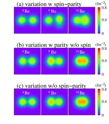
Figure 1: (color online) Density distribution of the intrinsic wave functions of the ground states of ⁸Be, ⁹Be, and ¹⁰Be obtained by (a) the AMD+VAP (variation after the angular-momentum and parity projections), (b) the variation after the parity projection without the angular-momentum projection, and (c) the variation without the angular-momentum and parity projections.

IV.3 Excited states

To investigate dipole excitations, I calculate $J^{\pi}=1^{-}$ states of ⁸Be and ¹⁰Be, and $J^{\pi}=1/2^{+}$, $3/2^{+}$, and $5/2^{+}$ states of ⁹Be by applying the sAMD and the sAMD+$\alpha$GCM based on the obtained ground state wave functions. For the sAMD, the shift parameter $\epsilon$ is taken to be $\epsilon=0.1$ fm which is small enough to give the $\epsilon$-independent result. For unit vectors $\boldsymbol{e}_{\sigma}$, I choose three sets, $\boldsymbol{e}_{\sigma=x,y,z}$, $\boldsymbol{e}_{\sigma=1,\ldots,8}$, and $\boldsymbol{e}_{\sigma=1,\ldots,14}$, and check the convergence of the dipole strengths. Here, the set of 8 vectors are $\boldsymbol{e}_{\sigma=1,\ldots,8}=(\pm 1/\sqrt{3},\pm 1/\sqrt{3},\pm 1/\sqrt{3})$, and that of 14 vectors are $\boldsymbol{e}_{\sigma=1,\ldots,14}=(\pm 1/\sqrt{3},\pm 1/\sqrt{3},\pm 1/\sqrt{3})$, $(\pm 1,0,0)$, $(0,\pm 1,0)$, and $(0,0,\pm 1)$. The $x$, $y$, and $z$ axes are taken to be the principle axes of the inertia of the intrinsic state that satisfy $\langle x^{2}\rangle\geq\langle y^{2}\rangle\geq\langle z^{2}\rangle$ and $\langle xy\rangle=\langle yz\rangle=\langle zx\rangle=0$. For the E1 strength, the sAMD model space with $\boldsymbol{e}_{\sigma=x,y,z}$ can cover $\boldsymbol{r}_{j}\phi_{{\boldsymbol{X}}_{i}}({\boldsymbol{r}_{j}})$ configurations excited by the E1 operator. However, for the ISD strength, a larger number of unit vectors ($\boldsymbol{e}_{\sigma}$) are necessary for the sAMD model space to cover $r_{j}^{2}\boldsymbol{r}_{j}\phi_{{\boldsymbol{X}}_{i}}({\boldsymbol{r}_{j}})$ configurations excited by the ISD operator. The E1 and ISD strengths of ⁹Be and ¹⁰Be calculated by the sAMD in three cases, $\boldsymbol{e}_{\sigma=x,y,z}$, $\boldsymbol{e}_{\sigma=1,\ldots,8}$, and $\boldsymbol{e}_{\sigma=1,\ldots,14}$, are shown in Fig. 2. As expected, the set $\boldsymbol{e}_{\sigma=x,y,z}$ is enough only for the E1 strength but not for the ISD strength. It is found that the set $\boldsymbol{e}_{\sigma=1,\ldots,8}$ is practically enough to get a qualitatively converged result for both the E1 and ISD strengths, and therefore this set is adopted in the present calculation of the dipole strengths. For the $\alpha$GCM calculation, the distance parameter is taken to be $\Delta D=-1,1,2,\ldots,20$ fm. This means that $\alpha$-cluster continuum states are treated as discretized states in the box boundary $\Delta D\leq 20$ fm.

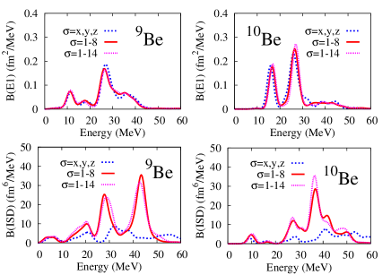
Figure 2: (color online) E1 and ISD strengths of ⁹Be and ¹⁰Be obtained by the sAMD in three cases of $\boldsymbol{e}_{\sigma=x,y,z}$, $\boldsymbol{e}_{\sigma=1,\ldots,8}$, and $\boldsymbol{e}_{\sigma=1,\ldots,14}$. The smearing width is $\gamma=2$ MeV.

The model space of the sAMD+$\alpha$GCM wave function given in Eq. (18) covers 1p-1h excitations and $\alpha$-cluster excitations from the ground state wave function. For the detailed description of the low-lying energy spectra and their dipole transition strengths, I mix additional configurations optimized for the low-lying levels ⁹Be$(1/2^{+}_{1})$, ⁹Be$(3/2^{+}_{1})$, ⁹Be$(5/2^{+}_{1})$ and ¹⁰Be$(1^{-}_{1})$, which are obtained by the AMD+VAP with $J^{\pi}=1/2^{+}$, $3/2^{+}$, and $5/2^{+}$ for ⁹Be and that with $J^{\pi}=1^{-}$ for ¹⁰Be. The final wave function with these additional VAP configurations is given as

$$\Psi^{\textrm{sAMD+}\alpha\textrm{GCM+cfg}}_{{\rm Be}(J^{\pi}_{k})} = \sum_{K}c_{0}(J^{\pi}_{k};K)P^{J\pi}_{MK}\Phi_{\rm AMD}({\bf Z}^{0})$$

$$+\sum_{i=1,\ldots,A}\sum_{\sigma}\sum_{K}c_{1}(J^{\pi}_{k};i,\sigma,K)P^{J\pi}_{MK}\Phi_{\rm AMD}({\bf Z}_{\rm nonflip}^{0}(i,\sigma))$$

$$+\sum_{i=1,\ldots,A}\sum_{\sigma}\sum_{K}c_{2}(J^{\pi}_{k};i,\sigma,K)P^{J\pi}_{MK}\Phi_{\rm AMD}({\bf Z}_{\rm flip}^{0}(i,\sigma))$$

$$+\sum_{\Delta D}\sum_{K}c_{3}(J^{\pi}_{k};\Delta D,K)P^{J\pi}_{MK}\Phi_{\rm AMD}(\boldsymbol{Z}^{0}_{D_{\alpha}}(\Delta D))$$

$$+ \sum_{J^{\prime}\pi^{\prime}}\sum_{K}c_{4}(J^{\pi}_{k};J^{\prime}\pi^{\prime},K)P^{J\pi}_{MK}\Phi_{\rm AMD}(\boldsymbol{Z}^{J^{\prime}\pi^{\prime}}_{\textrm{VAP}}).$$ (30)

The dipole strengths are calculated by the following matrix elements,

$$\langle\Psi^{\textrm{sAMD}}_{{\rm Be}(J^{\pi}_{k})}||{\cal M}||\Psi^{\textrm{sAMD}}_{{\rm Be}(\textrm{g.s.})}\rangle,$$ (31)

$$\langle\Psi^{\textrm{sAMD+}\alpha\textrm{GCM}}_{{\rm Be}(J^{\pi}_{k})}||{\cal M}||\Psi^{\textrm{sAMD+}\alpha\textrm{GCM}}_{{\rm Be}(\textrm{g.s.})}\rangle,$$ (32)

$$\langle\Psi^{\textrm{sAMD+}\alpha\textrm{GCM+cfg}}_{{\rm Be}(J^{\pi}_{k})}||{\cal M}||\Psi^{\textrm{sAMD+}\alpha\textrm{GCM+cfg}}_{{\rm Be}(\textrm{g.s.})}\rangle.$$ (33)

The calculated dipole strengths with and without the additional VAP configurations are found to be almost consistent with each other except for quantitative details of the energy position and the strengths in $E\leq 10$ MeV. In this paper, I mainly discuss the dipole strengths calculated by the sAMD and the sAMD+$\alpha$GCM+cfg wave functions, which I call cal-I and cal-II, respectively. The former corresponds to the small amplitude calculation containing 1p-1h excitations. The latter contains the large amplitude $\alpha$-cluster mode in addition to the 1p-1h excitations described by the sAMD model space. Namely, the sAMD+$\alpha$GCM+cfg includes the higher correlation than the sAMD in both the ground and excited states.

IV.4 E1 strength

The energy-weighted E1 strength of ⁹Be and ¹⁰Be obtained by the sAMD (cal-I) and the sAMD+$\alpha$GCM+cfg (cal-II) is shown in Fig. 3. The strength functions of two calculations (I) and (II) are qualitatively similar to each other except for broadening of the low-energy strength in $E\leq 15$ MeV of ⁹Be in the cal-II. The calculated EWS of the E1 strength is enhanced from the TRK sum rule value by a factor $1.7-1.8$. Figure 4 shows the comparison of the calculated E1 cross section with the experimental photonuclear cross sections of ⁹Be. The calculation reasonably describes the global feature of the experimental cross sections consisting of the low-energy strength in $E<20$ MeV and the GDR in $E>20$ MeV, though it somewhat overestimates the GDR peak energy and strength.

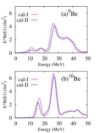
Figure 3: (color online) Energy-weighted E1 strength of ⁹Be and ¹⁰Be obtained by the sAMD (cal-I) and the sAMD+$\alpha$GCM+cfg (cal-II). The smearing width is $\gamma=2$ MeV.

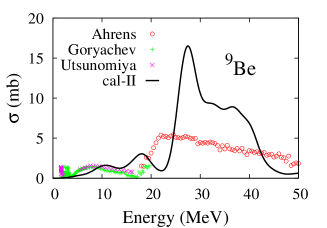
Figure 4: (color online) Comparison of the calculated E1 cross section of ⁹Be with the experimental photonuclear cross sections. The calculated values are those obtained with the sAMD+$\alpha$GCM+cfg (cal-II), smeared by $\gamma=2$ MeV. The experimental data are taken from the photonuclear cross sections by Ahrens et al.Ahrens:1975rq , the bremsstrahlung data by Goryachev et al.Goryachev92 , and the photodisintegration cross sections by Utsunomiya et al.Utsunomiya15 .

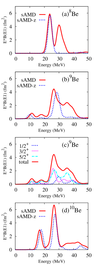
Figure 5: (color online) Energy-weighted E1 strength of ⁸Be, ⁹Be, and ¹⁰Be obtained by the sAMD ($\sigma=1,\ldots,8$) and the sAMD-z (longitudinal mode: $\sigma=z$) calculations. The sAMD and sAMD-z results for (a)⁸Be, (b)⁹Be, and (d)¹⁰Be are shown by solid and dashed lines, respectively. The decomposition of the strengths for $J^{\pi}=1/2^{+}$, $3/2^{+}$, and $5/2^{+}$ states of ⁹Be is also shown as well as the total strength in the panel (c). The smearing width is $\gamma=2$ MeV.

As shown in the comparison of the sAMD (cal-I) and the sAMD+$\alpha$GCM+cfg (cal-II) in Fig. 3, the E1 strength of ⁹Be and ¹⁰Be is not affected so much by the coupling with the large amplitude $\alpha$-cluster motion. In the following, we give detailed analysis of the E1 strength of ⁸Be, ⁹Be, and ¹⁰Be based on the sAMD to discuss effects of excess neutrons on the E1 strength in ⁹Be and ¹⁰Be. Figure 5 shows the E1 strength of ⁸Be, ⁹Be, and ¹⁰Be calculated by the sAMD. For ⁹Be, decomposition of the transition strength to $J=1/2^{+}$, $3/2^{+}$, and $5/2^{+}$ states is also shown. The GDR in ⁸Be shows a two peak structure in $E=20-40$ MeV. Also in ⁹Be, the two peak structure of the GDR is seen but it somewhat broadens. In addition to the GDR, low-lying E1 strength appears in $E=10-20$ MeV of ⁹Be. In ¹⁰Be, the lower peak of the GDR exists at $E\sim 25$ MeV, whereas the higher peak of the GDR is largely fragmented. Below the GDR, an E1 resonance appears at $E\sim 15$ MeV.

The origin of the two-peak structure of the GDR in Be isotopes is the prolate deformation of the $2\alpha$ core. To distinguish the longitudinal mode in the intrinsic frame, we calculate the E1 strength in the truncated sAMD model space by using wave functions shifted only to the longitudinal ($z$) direction, that is, the sAMD with the fixed $\sigma=z$ as

$$\Psi^{\textrm{sAMD-z}}_{{\rm Be}(J^{\pi}_{k})} = c_{0}(J^{\pi}_{k})P^{J\pi}_{MK}\Phi_{\rm AMD}({\bf Z}^{0})$$ (35)

$$+\sum_{i=1,\ldots,A}(c_{1}(J^{\pi}_{k};i)P^{J\pi}_{M0}\Phi_{\rm AMD}({\bf Z}_{\rm nonflip}^{0}(i,z))+c_{2}(J^{\pi}_{k};i)P^{J\pi}_{M0}\Phi_{\rm AMD}({\bf Z}_{\rm flip}^{0}(i,z)),$$

where the coefficients $c_{0}$, $c_{1}$, and $c_{2}$ are determined by diagonalization of the norm and Hamiltonian matrices. Here I omit the $K$-mixing and fix $K=0$ for ⁸Be and ¹⁰Be, and $K=3/2$ for ⁹Be to take into account only the $Y^{1}_{0}$ mode in the intrinsic frame. The sAMD with $\sigma=z$, which I call “sAMD-z”, is approximately regarded as the calculation containing the longitudinal mode but no transverse mode, though two modes do not exactly decouple from each other because of the angular-momentum projection. The E1 strength obtained by the sAMD-z is shown by dashed lines in Fig. 5(a), (b), and (d). In comparison of the sAMD and sAMD-z results, it is found that the lower peak of the GDR at $E=20-30$ MeV is contributed by the longitudinal mode of the $2\alpha$ core, whereas the higher peak of the GDR comes from the transverse mode. The higher peak broadens in ⁹Be and it is largely fragmented in ¹⁰Be indicating that the transverse mode is affected by excess neutrons. For the low-lying E1 resonances below the GDR, the strength at $E\sim 10$ MeV in ⁹Be and that at $E\sim 15$ MeV in ¹⁰Be are mainly contributed by the longitudinal mode. These low-energy dipole resonances in ⁹Be and ¹⁰Be are understood by the longitudinal motion of valence neutrons against the $2\alpha$ core.

From the above analysis of the E1 strength of ⁹Be and ¹⁰Be compared with that of ⁸Be, the effects of excess neutrons on the E1 strength is understood as follows. The longitudinal and transverse dipole modes in the $2\alpha$ core part contribute to the GDR with the two peak structure. The valence neutron modes couple with the transverse dipole mode of the $2\alpha$ core and they broaden the higher peak of the GDR. Moreover, the valence neutron modes against the $2\alpha$ core contribute to the low-energy E1 strength. More details of the low-energy dipole excitations are discussed later.

IV.5 ISD strength and coupling with the $\alpha$-cluster mode in ⁹Be and ¹⁰Be

As previously mentioned, the sAMD (cal-I) corresponds to the small amplitude calculation, whereas the sAMD+$\alpha$GCM+cfg (cal-II) contains the large amplitude $\alpha$-cluster mode. A possible enhancement of the ISD strength in the cal-II relative to the cal-I can be a good probe for the dipole excitation that couples with the $\alpha$-cluster mode, because the $\alpha$-cluster excitation in ⁹Be and ¹⁰Be involves the compressive dipole mode. The energy-weighted ISD strength of ⁹Be and ¹⁰Be calculated by the cal-I and cal-II is shown in Fig. 6. The strength of the isoscalar GDR in $E=30\sim 50$ MeV is not affected by the $\alpha$-cluster mode, whereas the ISD strength for some low-energy resonances are significantly enhanced in the cal-II as a result of the coupling with the $\alpha$-cluster mode. In ⁹Be, the ISD strength in $E<10$ MeV is remarkably enhanced in the cal-II, whereas the resonance at $E=10-15$ MeV has the weak ISD strength in both the cal-I and cal-II. In ¹⁰Be, the ISD strength around $E=15$ MeV is enhanced.

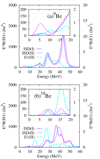
Figure 6: (color online) ISD strength of ⁹Be and ¹⁰Be obtained by the sAMD (cal-I) and the sAMD+$\alpha$GCM+cfg (cal-II). E1 strength obtained by the the sAMD+$\alpha$GCM+cfg (cal-II) is also shown for comparison. The smearing width is $\gamma=2$ MeV.

IV.6 Low-energy dipole resonances in ⁹Be and ¹⁰Be

Table 1: EWS of the E1 and ISD strengths for low-energy resonances: A1($E<8$ MeV), A2($8<E<15$ MeV), and A3($15<E<20$ MeV) in ⁹Be, and B1($E<12$ MeV) and B2($12<E<20$ MeV) in ¹⁰Be. The total EWS is also shown. The strengths are calculated by the sAMD (cal-I) and the sAMD+$\alpha$GCM+cfg (cal-II). The EWS calculated by the matrix elements for the transitions from the sAMD+$\alpha$GCM+cfg initial states to the sAMD final states (cal-III), and that for the transitions from the sAMD initial states to sAMD+$\alpha$GCM+cfg the final states (cal-IV) are also listed. The unit of $S(E1)$ is fm²MeV and that of $S(ISD)$ is fm⁶MeV.

	(I)	(II)	(III)	(IV)
$\alpha$ mode in initial	w/o	w	w	w/o
$\alpha$ mode in final	w/o	w	w/o	w
9Be
$S(E1;\textrm{total})$	58	56	58	56
$S(E1;\textrm{A1})$	0.13	0.43	0.39	0.16
$S(E1;\textrm{A2})$	3.3	2.4	2.6	3.5
$S(E1;\textrm{A3})$	2.7	3.3	3.3	2.6
$S(IS1;\textrm{total})$	$15.2\times 10^{3}$	$15.3\times 10^{3}$	$15.2\times 10^{3}$	$15.3\times 10^{3}$
$S(IS1;\textrm{A1})$	93	410	58	124
$S(IS1;\textrm{A2})$	108	230	200	131
$S(IS1,\textrm{A3})$	490	560	640	520
10Be
$S(E1;\textrm{total})$	63	62	63	62
$S(E1;\textrm{B1})$	0.09	0.08	0.06	0.10
$S(E1;\textrm{B2})$	10.4	8.7	7.6	10.9
$S(IS1;\textrm{total})$	$12.7\times 10^{3}$	$13.0\times 10^{3}$	$12.7\times 10^{3}$	$13.0\times 10^{3}$
$S(IS1;\textrm{B1})$	162	157	115	187
$S(IS1;\textrm{B2})$	56	187	83	74

From the analysis of the E1 and ISD strengths, the low-energy dipole excitations below the GDR in ⁹Be can be categorized as three resonances in $E<8$ MeV, $8<E<15$ MeV, and $15<E<20$ MeV, which I label A1, A2, and A3 resonances, respectively. The EWS in the corresponding energy regions, $S(E1/IS1;\textrm{A1})$, $S(E1/IS1;\textrm{A2})$, $S(E1/IS1;\textrm{A3})$, is listed in Table 1 as well as the total EWS value. In addition to the EWS obtained by the sAMD (cal-I) and sAMD+$\alpha$GCM+cfg (cal-II), the EWS calculated by the matrix elements

$$\langle\Psi^{\textrm{sAMD}}_{{\rm Be}(J^{\pi}_{k})}|{\cal M}|\Psi^{\textrm{sAMD+}\alpha\textrm{GCM+cfg}}_{{\rm Be}(\textrm{g.s.})}\rangle$$ (36)

for the transitions from the sAMD+$\alpha$GCM+cfg initial states to the sAMD final states (cal-III) and that by the matrix elements

$$\langle\Psi^{\textrm{sAMD+}\alpha\textrm{GCM+cfg}}_{{\rm Be}(J^{\pi}_{k})}|{\cal M}|\Psi^{\textrm{sAMD}}_{{\rm Be}(\textrm{g.s.})}\rangle$$ (37)

for the transitions from the sAMD initial states to the sAMD+$\alpha$GCM+cfg final states (cal-IV) are also shown in the table. The cal-III contains the $\alpha$-cluster mode in the initial states as the ground state correlation but not in the final states, whereas the cal-IV contains the $\alpha$-cluster mode only in the final states but not in the initial states. In all the calculations (I), (II), (III), and (IV), $S(E1;\textrm{A1})$ is very small, whereas $S(E1;\textrm{A2})$ and $S(E1;\textrm{A3})$ are significantly large as $\sim$10% of the TRK sum rule. Consequently, the EWS of the E1 strength in $E<20$ MeV exhausts $\sim$20% of the TRK sum rule and it is $\sim$10% of the calculated total EWS.

The $\alpha$-cluster mode does not affect so much the E1 and ISD strengths of A2 and those of A3, but it gives significant enhancement of the dipole strengths of A1. In particular, $S(IS1;\textrm{A1})$ is remarkably enhanced by the coupling with the $\alpha$-cluster mode. The enhancement is found only in the cal-II but not in other calculations, cal-I, cal-III, and cal-IV. It indicates that the coupling with the $\alpha$-cluster mode in the ground state and that in the A1 resonance coherently enhance $S(IS1;\textrm{A1})$. The $\alpha$-cluster mode also makes $S(E1;\textrm{A1})$ three times larger in the cal-II than the cal-I, though it is still less than 2% of the TRK sum rule.

As seen in the EWS of the sAMD+$\alpha$GCM+cfg (cal-II) in Table 1, the A1 resonance shows the relatively strong ISD and weak E1 transitions, whereas the A2 resonance shows the relatively weak ISD and strong E1 transitions. These characteristics of the A1 and A2 resonances can be understood by the $2\alpha+n$ picture as follows. The ground and low-lying states of ⁹Be are approximately described by the molecular orbital structure, where the valence neutron occupies molecular orbitals formed by the linear combination of $p$ orbits around $\alpha$ clusters Okabe77 ; Okabe78 ; SEYA ; OERTZENa . Let me consider two $\alpha$ clusters at the left and right along the $z$ axis (see Fig. 8). I call the left(right) $\alpha$ “$\alpha_{L(R)}$”, and label single-particle orbits (atomic orbitals) around each $\alpha$ cluster as $[Nn_{z}l_{z}j_{z}]_{\alpha_{L(R)}}$. Here $N$ is the total quantum (node) number, $n_{z}$ is the quantum number for the $z$-axis, and $l_{z}$ and $j_{z}$ are the $z$-components of the orbital- and total-angular momenta, respectively. The $\pi^{-}_{3/2}$ and $\pi^{+}_{3/2}$ molecular orbitals are given by the linear combination of the atomic orbitals $[101\frac{3}{2}]_{\alpha_{L,R}}$ as

$$\pi^{-}_{3/2}\equiv[101\frac{3}{2}]_{\textrm{MO}}=[101\frac{3}{2}]_{\alpha_{L}}+[101\frac{3}{2}]_{\alpha_{R}}$$ (38)

$$\pi^{+}_{3/2}\equiv[211\frac{3}{2}]_{\textrm{MO}}=[101\frac{3}{2}]_{\alpha_{L}}-[101\frac{3}{2}]_{\alpha_{R}}$$ (39)

where $[Nn_{z}l_{z}j_{z}]_{\textrm{MO}}$ is the label indicating the quantum numbers $N$, $n_{z}$, $l_{z}$, and $j_{z}$ of the molecular orbital around the $2\alpha$. Another molecular orbital is the longitudinal orbital $\sigma^{+}_{1/2}$ given by the linear combination of $[110\frac{1}{2}]_{\alpha_{L,R}}$ as

$$\sigma^{+}_{1/2}\equiv[220\frac{3}{2}]_{\textrm{MO}}=[110\frac{1}{2}]_{\alpha_{L}}-[110\frac{1}{2}]_{\alpha_{R}}.$$ (41)

In the case that the $\alpha$-$\alpha$ distance is not so large, the molecular orbital $[Nn_{z}l_{z}j_{z}]_{\textrm{MO}}$ approximately corresponds to the Nilsson (deformed shell-model) orbit $[Nn_{3}\Lambda]_{\Omega}$ with $n_{3}=n_{z}$, $\Lambda=l_{z}$, and $\Omega=j_{z}$ in the prolate deformation. $\pi^{-}_{3/2}$ is the negative-parity orbital with no node ($n_{z}=0$), $\pi^{+}_{3/2}$ is the positive-parity orbital with one node ($n_{z}=1$), and $\sigma^{+}_{1/2}$ is the positive-parity orbital with two nodes ($n_{z}=2$) along the $z$-axis.

For the valence neutron around the $2\alpha$, $\pi^{-}_{3/2}$ is the lowest negative-parity molecular orbital, whereas $\sigma^{+}_{1/2}$ is the lowest positive-parity orbital. The ground state of ⁹Be dominantly has the $2\alpha+n$ structure with the $\pi^{-}_{3/2}$ configuration. The A1 resonance is approximately described by the $\sigma^{+}_{1/2}$ configuration, whereas the A2 resonance is dominated by the $\pi^{+}_{3/2}$ configuration (see Fig. 8). The E1 transition for $\pi^{-}_{3/2}\to\pi^{+}_{3/2}$, i.e., $[101\frac{3}{2}]_{\textrm{MO}}\to[211\frac{3}{2}]_{\textrm{MO}}$ is possible because the $Y^{1}_{0}$ operator changes $N\to N\pm 1$ and $n_{z}\to n_{z}\pm 1$. However, the E1 transition for $\pi^{-}_{3/2}\to\sigma^{+}_{1/2}$, i.e., $[101\frac{3}{2}]_{\textrm{MO}}\to[220\frac{1}{2}]_{\textrm{MO}}$ is forbidden because the change $n_{z}\to n_{z}\pm 2$ is not possible for the E1 operator. This is the reason why the E1 strength is large for A2 but it is suppressed for A1. Because of the $[211\frac{3}{2}]_{\textrm{MO}}$ configuration of the A2 resonance, the E1 strength of A2 shows the $K=3/2$ band feature that the contribution from transitions to $J^{\pi}=3/2^{+}$ and $5/2^{+}$ states is dominant as seen in Fig. 5(c). The A1 resonance has the large node number $n_{z}=2$ along the $2\alpha$ direction than the A2 resonance ($n_{z}=1$), and therefore, the spatial development of the $2\alpha$ clustering is more prominent in the A1 resonance. As a result of the developed clustering, the A1 resonance couples rather strongly with the $\alpha$-cluster mode. The coupling with the $\alpha$-cluster mode, namely, the ⁵He-$\alpha$ relative motion in A1 enhances the ISD strength as discussed previously.

Let me discuss low-energy dipole resonances in ¹⁰Be. The low-energy dipole strength below the GDR can be categorized as two resonances in $E<12$ MeV and $12<E<20$ MeV, which I label B1 and B2, respectively. The EWS of the dipole strengths for the corresponding energy regions are listed in table 1. The B2 resonance shows the strong E1 transition exhausting more than 20% of the TRK sum rule and 10% of the calculated total EWS. It also shows the significant ISD strength enhanced by the $\alpha$-cluster mode in the cal-II (sAMD+$\alpha$GCM+cfg). The significant E1 strength and the strong coupling with the $\alpha$-cluster mode of the B2 resonance can be understood by two neutron correlation in the $2\alpha+2n$ picture as shown in the schematic figures of Fig. 8. The configuration in the ground state of ¹⁰Be is approximately described by the positive-parity projected state of the atomic orbital configuration as

$$[101\frac{3}{2}]_{\alpha_{L}}[10-1-\frac{3}{2}]_{\alpha_{L}}+[101\frac{3}{2}]_{\alpha_{R}}[10-1-\frac{3}{2}]_{\alpha_{R}}$$ (42)

$$=\frac{1}{2}\left\{(\pi^{-}_{3/2})^{2}+(\pi^{+}_{3/2})^{2})\right\},$$ (43)

which corresponds to the ⁶He+$\alpha$ cluster structure in the intrinsic state of the ¹⁰Be ground state. The B2 resonance is interpreted as the parity partner of the ground state as

$$[101\frac{3}{2}]_{\alpha_{L}}[10-1-\frac{3}{2}]_{\alpha_{L}}-[101\frac{3}{2}]_{\alpha_{R}}[10-1-\frac{3}{2}]_{\alpha_{R}}$$ (44)

$$=\frac{1}{2}\left\{\pi^{-}_{3/2}\pi^{+}_{3/2}+\pi^{+}_{3/2}\pi^{-}_{3/2}\right\}.$$ (45)

In the transition from the ground state to the B2 resonance, the coherent contribution of two neutrons enhances the E1 strength. The B2 resonance has a large overlap with negative-parity ⁶He+$\alpha$ cluster wave functions, for instance, 60% overlap with $P^{1-}_{00}\Phi_{\rm AMD}({\bf Z}^{0}_{D_{\alpha}}(\Delta D=1\textrm{fm}))$. As a result of the strongly coupling with the $\alpha$-cluster mode, the ISD strength of the B2 resonance is enhanced. In other words, the B2 resonance is regarded as the $\alpha$-cluster excitation on the ground state which already contains the ⁶He+$\alpha$ cluster structure. In contrast to the B2 resonance, the B1 resonance is regarded as a single-particle excitation with the molecular orbital configuration $\pi^{-}_{3/2}\sigma^{+}_{1/2}$ and has no coherent contribution of two neutrons to the E1 strength. Moreover, the $\pi^{-}_{3/2}\sigma^{+}_{1/2}$ configuration contains the ⁵He+⁵He and ⁶He^∗+$\alpha$ components instead of the ⁶He+$\alpha$ component, and therefore, it does not couple with the $\alpha$-cluster mode.

Finally, I discuss the calculated $B(E1)$ of the $1/2^{+}_{1}$, $3/2^{+}_{1}$, and $5/2^{+}_{1}$ states of ⁹Be, which contribute to the dipole strengths of the A1 resonance. In Fig. 7, I show the E1 strength in $E\leq 10$ MeV of ⁹Be. Here the smearing width is chosen to be $\gamma=0.1$ MeV to resolve discrete states. The $1/2^{+}_{1}$, $3/2^{+}_{1}$, and $5/2^{+}_{1}$ states are obtained as discrete states in the sAMD (cal-I). In the sAMD+$\alpha$GCM+cfg (cal-II), the $1/2^{+}_{1}$ and $5/2^{+}_{1}$ states are still discrete states, however, the $3/2^{+}_{1}$ shows a resonance behavior coupling with the discretized continuum states in the box boundary at $\Delta D\leq 20$ fm. We evaluate the $B(E1)$ of the $3/2^{+}_{1}$ resonance by a sum of the E1 strength in $E<6$ MeV and estimate the excitation energy by the $B(E1)$ weighted averaged energy of $3/2^{+}$ states in this energy region. In Table 2, I compare the calculated E1 strength of the $1/2^{+}_{1}$, $3/2^{+}_{1}$, and $5/2^{+}_{1}$ states with the experimental values measured by the $(\gamma,n)$ cross sections in Ref. Arnold:2011nv . The excitation energies and $B(E1)$ of the ⁹Be($5/2^{+}_{1}$) and ⁹Be($3/2^{+}_{1}$) obtained by the sAMD+$\alpha$GCM+cfg (cal-II) reproduce reasonably the experimental data. However, the calculated $B(E1)$ of the ⁹Be($1/2^{+}_{1}$) is quite small inconsistently to the experimental data. The $1/2^{+}_{1}$ state has been suggested to be a virtual or resonance state of a $s$-wave neutron Efros:1998yk ; Arai:2003jm ; Burda:2010an ; Garrido:2010xz ; AlvarezRodriguez:2010ng ; Efros:2013zoa ; Odsuren:2015pja . However, the present model is insufficient to describe such the virtual or $s$-wave resonance state because the valence neutron motion far from the $2\alpha$ is not taken into account in the model space.

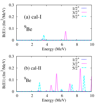
Figure 7: (color online) E1 strength of $1/2^{+}$, $3/2^{+}$, and $5/2^{+}$ states of ⁹Be in $E<10$ MeV obtained by (a) the sAMD (cal-I) and (b) the sAMD+$\alpha$GCM+cfg (cal-II). The smearing width is $\gamma=0.1$ MeV.

Table 2: Excitation energy and E1 strength of ⁹Be($1/2^{+}_{1}$), ⁹Be($3/2^{+}_{1}$), ⁹Be($5/2^{+}_{1}$), and ¹⁰Be($1^{-}_{1}$). The energy (MeV) and $B(E1)$ (fm²) calculated by the sAMD (cal-I) and the sAMD+$\alpha$GCM+cgf (cal-II) are listed compared with the experimental data. The experimental values of ⁹Be are data measured by the $(\gamma,n)$ cross sections in Ref. Arnold:2011nv . The experimental excitation energy of ¹⁰Be($1^{-}$) is taken from Refs. AjzenbergSelove:1988ec ; Tilley:2004zz .

	cal-I		cal-II		exp
	$E$	$B(E1)$	$E$	$B(E1)$	$E$	$B(E1)$
9Be
$1/2^{+}$	3.5	0.002	2.9	0.002	1.731(2)	0.136(2)
$3/2^{+}$	6.5	0.014	5.1	0.039	4.704	0.068(7)
$5/2^{+}$	3.6	0.008	3.1	0.013	3.008(4)	0.016(2)
10Be
$1^{-}$	9.8	0.009	8.3	0.010	5.960

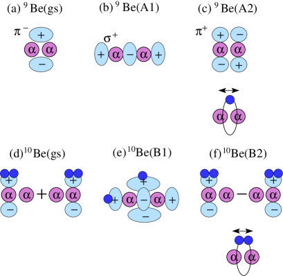
Figure 8: (color online) Schematic figures of $2\alpha$ and valence neutrons for the ground state and the A1 and A2 resonances of ⁹Be, and those for the ground state and the B1 and B2 resonances of ¹⁰Be.

V Summary

I investigated the isovector and isoscalar dipole excitations in ⁹Be and ¹⁰Be with the shifted AMD combined with the $\alpha$-cluster GCM, in which the 1p-1h excitations on the ground state and the large amplitude $\alpha$-cluster mode are incorporated. Since the angular-momentum and parity projections are done, the coupling of excitations in the intrinsic frame with the rotation and parity transformation is taken into account microscopically. The low-energy E1 resonances appear in $E<20$ MeV because of valence neutron modes against the $2\alpha$ core. They exhaust about $20\%$ of the TRK sum rule and $10\%$ of the calculated EWS. The GDR shows the two peak structure which is understood by the E1 excitations in the 2$\alpha$ core part with the prolate deformation. The higher peak of the GDR for the transverse mode broadens in ⁹Be and it is largely fragmented in ¹⁰Be because of excess neutrons.

By comparing the results of the shifted AMD combined with and without the $\alpha$-cluster GCM, I investigated how the E1 and ISD strengths in ⁹Be and ¹⁰Be are affected by the large amplitude $\alpha$-cluster mode. The ISD strength is a good probe to identify the dipole resonances that couples with the $\alpha$-cluster mode because the $\alpha$-cluster mode in ⁹Be and ¹⁰Be involves the compressive dipole mode. It was found that the ISD strength for some low-energy resonances in ⁹Be and ¹⁰Be are enhanced by the coupling with the $\alpha$-cluster mode, whereas the E1 strength is not so sensitive to the coupling with the $\alpha$-cluster mode. In ⁹Be, the ISD strength of the low-energy resonance in $E<10$ MeV is remarkable. In ¹⁰Be, the ISD strength at $E\sim 15$ MeV is enhanced by the coupling with the $\alpha$-cluster mode. This resonance at $E\sim 15$ MeV in ¹⁰Be is regarded as the $\alpha$-cluster excitation on the ground state having the ⁶He+$\alpha$ structure and can be interpreted as the parity partner of the ground state. The E1 transition of this resonance is also strong because of the coherent contribution of two valence neutrons.

The calculated E1 strength of ⁹Be reasonably describes the global feature of experimental photonuclear cross sections consisting of the low-energy strength in $E<20$ MeV and the GDR in $E>20$ MeV, though it somewhat overestimates the GDR peak energy and its strength. For the low-lying positive-parity states of ⁹Be, the calculated excitation energies and $B(E1)$ of the ⁹Be($5/2^{+}_{1}$) and ⁹Be($3/2^{+}_{1}$) reasonably agree to the experimental data. However, the calculation fails to reproduce the experimental $B(E1)$ of the ⁹Be($1/2^{+}_{1}$) because the present model is insufficient to describe the detailed asymptotic behavior of the $s$-wave neutron in the $1/2^{+}_{1}$ state.

References

- (1) T. Kobayashi et al. Phys. Lett. B232, 51 (1989).
- (2) K. Ieki et al., Phys. Rev. Lett. 70, 730 (1993).
- (3) D. Sackett et al., Phys. Rev. C 48, 118 (1993).
- (4) S. Shimoura et al., Phys. Lett. B 348, 29 (1995).
- (5) M. Zinser et al., Nucl. Phys. A 619, 151 (1997).
- (6) T. Aumann et al., Phys. Rev. C 59, 1252 (1999).
- (7) T. Nakamura et al., Phys. Rev. Lett. 96, 252502 (2006).
- (8) R. Kanungo et al., Phys. Rev. Lett. 114, no. 19, 192502 (2015).
- (9) D. J. Millener, J. W. Olness, E. K. Warburton and S. S. Hanna, Phys. Rev. C 28, 497 (1983).
- (10) R.Palit et al., Phys. Rev. C 68, 034318 (2003).
- (11) T.Nakamura et al., Phys. Lett. 394B, 11 (1997).
- (12) N. Fukuda et al., Phys. Rev. C 70, 054606 (2004).
- (13) P. G. Hansen and B. Jonson, Europhys. Lett. 4, 409 (1987).
- (14) G. Bertsch and J. Foxwell, Phys. Rev. C 41, 1300 (1990) [Phys. Rev. C 42, 1159 (1990)].
- (15) Y. Suzuki and Y. Tosaka, Nucl. Phys. A 517, 599 (1990).
- (16) M.Honma, H.Sagawa Prog. Theor. Phys. 84, 494 (1990).
- (17) G. F. Bertsch and H. Esbensen, Annals Phys. 209, 327 (1991).
- (18) H.Sagawa, N.Takigawa, Nguyen van Giai Nucl.Phys. A543, 575 (1992).
- (19) A. Csoto, Phys. Rev. C 49, 3035 (1994).
- (20) T.Suzuki, H.Sagawa and P.F.Bortignon Nucl. Phys. A662, 282 (2000).
- (21) E. Garrido, D. V. Fedorov and A. S. Jensen, Nucl. Phys. A 708, 277 (2002).
- (22) T. Myo, S. Aoyama, K. Kato and K. Ikeda, Phys. Lett. B 576 (2003) 281.
- (23) L. V. Chulkov et al., Nucl. Phys. A 759, 23 (2005).
- (24) C. A. Bertulani and M. S. Hussein, Phys. Rev. C 76, 051602 (2007).
- (25) K. Hagino and H. Sagawa, Phys. Rev. C 76, 047302 (2007).
- (26) K. Hagino, H. Sagawa, T. Nakamura and S. Shimoura, Phys. Rev. C 80, 031301 (2009).
- (27) D. Baye, P. Capel, P. Descouvemont and Y. Suzuki, Phys. Rev. C 79, 024607 (2009).
- (28) Y. Kikuchi, K. Kato, T. Myo, M. Takashina and K. Ikeda, Phys. Rev. C 81, 044308 (2010).
- (29) E. C. Pinilla, P. Descouvemont and D. Baye, Phys. Rev. C 85, 054610 (2012).
- (30) Y. Kikuchi, T. Myo, K. Kato and K. Ikeda, Phys. Rev. C 87, no. 3, 034606 (2013).
- (31) T.Myo, A.Ohnishi and K.Kato, Prog. Theor. Phys. 99, 801 (1998)
- (32) H. Sagawa, T. Suzuki, H. Iwasaki and M. Ishihara, Phys. Rev. C 63, 034310 (2001).
- (33) M. Tohyama, Phys.Lett. 323B, 257 (1994).
- (34) I.Hamamoto, H.Sagawa and X.Z.Zhang, Phys.Rev. C 53, 765 (1996).
- (35) I.Hamamoto and H.Sagawa, Phys.Rev. C 53, R1492 (1996).
- (36) H. Sagawa and T. Suzuki, Phys. Rev. C 59, 3116 (1999).
- (37) G. Colo and P. F. Bortignon, Nucl. Phys. A 696, 427 (2001).
- (38) T. Nakatsukasa and K. Yabana, Phys. Rev. C 71, 024301 (2005).
- (39) Y. Kanada-En’yo and M. Kimura, Phys. Rev. C 72, 064301 (2005).
- (40) P. Van Isacker, M. A. Nagarajan and D. D. Warner, Phys. Rev. C 45, R13 (1992).
- (41) F.Catara, E.G.Lanza, M.A.Nagarajan and A.Vitturi, Nucl. Phys. A624, 449 (1997).
- (42) M. Matsuo, Nucl. Phys. A 696, 371 (2001).
- (43) D. Vretenar, N. Paar, P. Ring and G. A. Lalazissis, Nucl. Phys. A 692, 496 (2001).
- (44) S. Goriely and E. Khan, Nucl. Phys. A 706, 217 (2002).
- (45) N. Paar, P. Ring, T. Niksic and D. Vretenar, Phys. Rev. C 67, 034312 (2003).
- (46) N. Tsoneva, H. Lenske and C. Stoyanov, Phys. Lett. B 586, 213 (2004).
- (47) M. Matsuo, K. Mizuyama and Y. Serizawa, Phys. Rev. C 71, 064326 (2005).
- (48) J. Piekarewicz, Phys. Rev. C 73, 044325 (2006).
- (49) J. Terasaki and J. Engel, Phys. Rev. C 74, 044301 (2006).
- (50) J. Liang, L. G. Cao and Z. Y. Ma, Phys. Rev. C 75, 054320 (2007).
- (51) N. Tsoneva and H. Lenske, Phys. Rev. C 77, 024321 (2008).
- (52) N. Paar, D. Vretenar, E. Khan and G. Colo, Rept. Prog. Phys. 70, 691 (2007).
- (53) K. Yoshida and N. Van Giai, Phys. Rev. C 78, 014305 (2008).
- (54) G. Co’, V. De Donno, C. Maieron, M. Anguiano and A. M. Lallena, Phys. Rev. C 80, 014308 (2009).
- (55) M. Martini, S. Peru and M. Dupuis, Phys. Rev. C 83, 034309 (2011).
- (56) T. Inakura, T. Nakatsukasa and K. Yabana, Phys. Rev. C 84, 021302 (2011).
- (57) X. Roca-Maza, G. Pozzi, M. Brenna, K. Mizuyama and G. Colo, Phys. Rev. C 85, 024601 (2012).
- (58) S. Ebata, T. Nakatsukasa and T. Inakura, Phys. Rev. C 90, no. 2, 024303 (2014).
- (59) S. Bacca, N. Barnea, G. Hagen, M. Miorelli, G. Orlandini and T. Papenbrock, Phys. Rev. C 90, no. 6, 064619 (2014).
- (60) J. Piekarewicz, Phys. Rev. C 83, 034319 (2011).
- (61) A. Carbone, G. Colo, A. Bracco, L. G. Cao, P. F. Bortignon, F. Camera and O. Wieland, Phys. Rev. C 81, 041301 (2010).
- (62) P.-G. Reinhard and W. Nazarewicz, Phys. Rev. C 87, no. 1, 014324 (2013).
- (63) T. Inakura, T. Nakatsukasa and K. Yabana, Phys. Rev. C 88, no. 5, 051305 (2013).
- (64) K. Govaert, F. Bauwens, J. Bryssinck, D. De Frenne, E. Jacobs, W. Mondelaers, L. Govor and V. Y. Ponomarev, Phys. Rev. C 57, 2229 (1998).
- (65) R.-D. Herzberg et al., Phys. Rev. C 60, 051307 (1999).
- (66) A. Leistenschneider et al., Phys. Rev. Lett. 86, 5442 (2001).
- (67) N. Ryezayeva et al., Phys. Rev. Lett. 89, 272502 (2002).
- (68) E. Tryggestad et al., Phys. Rev. C 67, 064309 (2003).
- (69) T. Hartmann, M. Babilon, S. Kamerdzhiev, E. Litvinova, D. Savran, S. Volz and A. Zilges, Phys. Rev. Lett. 93, 192501 (2004).
- (70) P. Adrich et al., Phys. Rev. Lett. 95, 132501 (2005).
- (71) J. Gibelin et al., Phys. Rev. Lett. 101, 212503 (2008).
- (72) A. Klimkiewicz et al., Phys. Rev. C 76, 051603 (2007).
- (73) R. Schwengner et al., Phys. Rev. C 78, 064314 (2008).
- (74) O. Wieland et al., Phys. Rev. Lett. 102, 092502 (2009).
- (75) J. Endres et al., Phys. Rev. C 80, 034302 (2009).
- (76) J. Endres et al., Phys. Rev. Lett. 105, 212503 (2010).
- (77) A. Tamii et al., Phys. Rev. Lett. 107, 062502 (2011).
- (78) B. L. Berman and S. C. Fultz, Rev. Mod. Phys. 47, 713 (1975).
- (79) M. J. Jakobson, Phys. Rev. 123, 229 (1961).
- (80) R.J. Hughes, R.H. Sambell, E.G. Muirhead, B.M. Spicer, Nucl. Phys., A238, 189 (1975).
- (81) A.M. Goryachev, G.N. Zalesnyy, I.V. Pozdnev, Izv. Rossiiskoi Akademii Nauk, Ser.Fiz. 56, 159 (1992).
- (82) H. Utsunomiya, Y. Yonezawa, H. Akimune, T. Yamagata, M. Ohta, M. Fujishiro, H. Toyokawa and H. Ohgaki, Phys. Rev. C 63, 018801 (2001).
- (83) C. W. Arnold, T. B. Clegg, C. Iliadis, H. J. Karwowski, G. C. Rich, J. R. Tompkins and C. R. Howell, Phys. Rev. C 85, 044605 (2012).
- (84) H. Ustunomiya et al., Phys. Rev. C, submitted.
- (85) J. Ahrens et al., Nucl. Phys. A 251, 479 (1975).
- (86) S. Okabe, Y. Abe and H. Tanaka, Prog. Theor. Phys. 57, 866 (1977).
- (87) S. Okabe and Y. Abe, Prog. Theor. Phys. 59, 315 (1978).
- (88) A. C. Fonseca, J. Revai, and A. Matveenko, Nucl. Phys. A326, 182 (1979).
- (89) P. Descouvemont, Phys. Rev. C 39, 1557 (1989).
- (90) K. Arai, Y. Ogawa, Y. Suzuki and K. Varga, Phys. Rev. C 54, 132 (1996).
- (91) V. D. Efros and J. M. Bang, Eur. Phys. J. A 4, 33 (1999).
- (92) K. Arai, P. Descouvemont, D. Baye and W. N. Catford, Phys. Rev. C 68, 014310 (2003).
- (93) O. Burda, P. von Neumann-Cosel, A. Richter, C. Forssen and B. A. Brown, Phys. Rev. C 82, 015808 (2010).
- (94) E. Garrido, D. V. Fedorov and A. S. Jensen, Phys. Lett. B 684, 132 (2010).
- (95) R. Alvarez-Rodriguez, A. S. Jensen, E. Garrido and D. V. Fedorov, Phys. Rev. C 82, 034001 (2010).
- (96) V. D. Efros et al. [European Centre for Theoretical Studies in Nuclear Physics and Related Areas Collaboration], Phys. Rev. C 89, no. 2, 027301 (2014).
- (97) M. Odsuren, Y. Kikuchi, T. Myo, M. Aikawa and K. Kato, Phys. Rev. C 92, no. 1, 014322 (2015).
- (98) A. Ono, H. Horiuchi, T. Maruyama and A. Ohnishi, Phys. Rev. Lett. 68, 2898 (1992).
- (99) A. Ono, H. Horiuchi, T. Maruyama and A. Ohnishi, Prog. Theor. Phys. 87, 1185 (1992).
- (100) Y. Kanada-En’yo, H. Horiuchi and A. Ono, Phys. Rev. C 52, 628 (1995).
- (101) Y. Kanada-En’yo and H. Horiuchi, Phys. Rev. C 52, 647 (1995).
- (102) Y. Kanada-En’yo and H. Horiuchi, Prog. Theor. Phys. Suppl. 142, 205 (2001).
- (103) Y. Kanada-En’yo, M. Kimura and A. Ono, PTEP 2012 01A202 (2012).
- (104) T. Furuta, K. H. O. Hasnaoui, F. Gulminelli, C. Leclercq and A. Ono, Phys. Rev. C 82 (2010) 034307.
- (105) Y. Kanada-En’yo, Phys. Rev. Lett. 81, 5291 (1998).
- (106) Y. Kanada-En’yo, H. Horiuchi and A. Dote, Phys. Rev. C 60, 064304 (1999).
- (107) Y. Kanada-En’yo, Prog. Theor. Phys. 117, 655 (2007) [Prog. Theor. Phys. 121, 895 (2009)].
- (108) Y. Kanada-En’yo, Phys. Rev. C 89, 024302 (2014).
- (109) H. Feldmeier, K. Bieler and J. Schnack, Nucl. Phys. A 586, 493 (1995).
- (110) T. Neff and H. Feldmeier, Nucl. Phys. A 713, 311 (2003).
- (111) T. Ando, K.Ikeda, and A. Tohsaki, Prog. Theor. Phys. 64, 1608 (1980).
- (112) R. Tamagaki, Prog. Theor. Phys. 39, 91 (1968).
- (113) N. Yamaguchi, T. Kasahara, S. Nagata, and Y. Akaishi, Prog. Theor. Phys. 62, 1018 (1979).
- (114) M. Seya, M. Kohno, and S. Nagata, Prog. Theor. Phys. 65, 204 (1981).
- (115) W. von Oertzen, Z. Phys. A 354, 37 (1996); 357, 355 (1997),
- (116) F. Ajzenberg-Selove, Nucl. Phys. A 490, 1 (1988).
- (117) D. R. Tilley, J. H. Kelley, J. L. Godwin, D. J. Millener, J. E. Purcell, C. G. Sheu and H. R. Weller, Nucl. Phys. A 745, 155 (2004).