The Early History of the Integrable Chiral Potts Model and the Odd-Even Problem

Abstract

In the first part of this paper I shall discuss the round-about way of how the integrable chiral Potts model was discovered about 30 years ago. As there should be more higher-genus models to be discovered, this might be of interest. In the second part I shall discuss some quantum group aspects, especially issues of odd versus even $N$ related to the Serre relations conjecture in our quantum loop subalgebra paper of 5 years ago and how we can make good use of coproducts, also borrowing ideas of Drinfeld, Jimbo, Deguchi, Fabricius, McCoy and Nishino.

Keywords: Chiral Potts model, Yang–Baxter equation, Star-triangle equation

1 Introduction

It is a great honor to be asked to contribute to the special issue honoring the 75th birthday of Professor Rodney Baxter and it may be proper to finally give a review of the early history of how the integrable chiral Potts model came into being. First of all, Baxter has given many important contributions to this topic, as is also evidenced by his contribution in this special issue [1]. Secondly, the early development of the theory went through many unexpected twists and turns and missed opportunities not reported in the published papers; reporting on these should encourage others seeking to discover new solvable models and further properties of existing ones.

2 Part 1: Early history of the integrable chiral Potts model

2.1 Discovery of the Yang–Baxter integrable chiral Potts model

It really started in the summer of 1986, when Barry McCoy, Mulin Yan, Helen Au-Yang and I decided to start a project on parafermions. The work of Zamolodchikov and Fateev [2] seemed to us to relate parafermionic conformal quantum field theory to the phase transition separating regimes I and II in the RSOS model of Andrews, Baxter and Forrester [3], especially, since Huse [4] had already suggested that this transition is in the universality class of the chiral clock model [5, 6]. We split the project into two parts: Au-Yang and Yan were to look at a preprint of Alcaraz and Lima Santos, now published as [7], while McCoy and I would try to find Painlevé-type equations that could be used to describe parafermionic correlations, extending the conformal theory into the massive regime, and also try a variety of perturbation expansions of correlation functions to use for that purpose.

Au-Yang soon discovered that the full 3-state self-dual case solves the quantum Lax pair equations, as formulated by Bashilov and Pokrovsky [8]: There are no conditions on the corresponding spin-chain Hamiltonian for a family of transfer matrices commuting with it to exist, even if the Boltzmann weights in [7] are allowed to be chiral! Chiral comes from the Greek word $\chi\epsilon\acute{\iota}\rho$, hand, so that it means handed, not reflection invariant. The four of us looked briefly at Au-Yang’s solution and found that the spectral variables lie on an elliptic curve, but that the only physical two-dimensional classical spin model was the three-state critical Potts model. McCoy and I decided for the moment to continue with Painlevé and series expansions.

Au-Yang and Yan went on to analyze the non-self-dual 3-state chiral Potts model with Boltzmann weights $W(a-b)$ and ${\overline{W}}(a-b)$ for horizontal and vertical nearest-neighbor pair interactions of spins $a$ and $b$ with values 1 to 3 (or 0 to 2) mod 3, writing

$$l_{n}={\displaystyle\sum_{j=0}^{N-1}\omega^{-jn}W(j)\over\displaystyle\sum_{j=0}^{N-1}W(j)},\qquad\bar{l}_{n}={{\overline{W}}(n)\over{\overline{W}}(0)},\qquad\omega=\mathrm{e}^{2\pi\mathrm{i}/N},\quad N=3,$$ (1)

as used in the quantum Lax pair approach. A logical thing to do seemed to rewrite the star-triangle equations [10, 11] in these variables, assuming three versions of the weights for the three different positions in these equations, namely $W$ and ${\overline{W}}$, $W^{\prime}$ and ${\overline{W}}{}^{\prime}$, or $W^{\prime\prime}$ and ${\overline{W}}{}^{\prime\prime}$. As $l_{n}$ involves a discrete Fourier transform, such a transform was also applied to the star-triangle equations, which then became, (with proper normalizations of all $W$’s and ${\overline{W}}$’s, which we can choose to be $\sum_{j=1}^{N-1}W(j)=\overline{W}(0)=1$),

$$V_{ab}\overline{X}_{b}=\overline{V}_{ba}X_{a}\;,$$ (2)

where

$$V_{ab}=\sum_{m=0}^{N-1}\sum_{k=0}^{N-1}\omega^{am+bk+mk}\,l^{\vphantom{y}}_{m}\bar{l}^{\prime}_{k}=\sum_{k=0}^{N-1}\omega^{bk}\,W(a+k){\overline{W}}{}^{\prime}(k),$$ (3)

$$\overline{V}_{ab}=\sum_{m=0}^{N-1}\sum_{k=0}^{N-1}\omega^{am+bk+mk}\,\bar{l}^{\vphantom{y}}_{m}l^{\prime}_{k}=\sum_{k=0}^{N-1}\omega^{ak}\,W(k){\overline{W}}{}^{\prime}(b+k),$$ (4)

and

$$X_{a}=\sum_{k=0}^{N-1}\omega^{ak}\,l^{\prime\prime}_{k}=\sum_{k=0}^{N-1}\omega^{ak}\,{\overline{W}}{}^{\prime\prime}(k),\qquad\overline{X}_{a}=\sum_{k=0}^{N-1}\omega^{ak}\,\bar{l}^{\prime\prime}_{k}=W^{\prime\prime}(a).$$ (5)

Eliminating $X$ and $\overline{X}$ from (2), one gets the consistency equations

$${V_{ab}V_{00}\over V_{0b}V_{a0}}={\overline{V}_{ba}\overline{V}_{00}\over\overline{V}_{0a}\overline{V}_{b0}}\;,\quad 1\leq a,b\leq N-1.$$ (6)

Note that no difference-variable assumption is made on rapidities (spectral variables). In the self-dual case $\bar{l}_{n}=l_{n}$, $\overline{V}_{ab}=V_{ab}$, one can restrict oneself to $a<b$; then for $N=3$ there is only one equation left and choosing $l_{1}$ and $l_{2}$ arbitrarily, the equation then determines a relation between $l^{\prime}_{1}$ and $l^{\prime}_{2}$, parametrizing a commuting family of transfer matrices.

More generally, assuming the existence of a one-parameter family of solutions leading to a commuting family of diagonal-to-diagonal transfer matrices $T(u)$, we should by Baxter’s well-known argument [12] take the derivative of the logarithm of $T(u)$ at a shift point $u=0$, where

$$l_{n}=\alpha_{n}u+\beta_{n}u^{2}+\mathrm{O}\left(u^{3}\right),\quad\bar{l}_{n}=\overline{\alpha}_{n}u+\bar{\beta}_{n}u^{2}+\mathrm{O}\left(u^{3}\right),$$ (7)

for $1\leq n\leq N-1$, $l_{0}=\bar{l}_{0}=1$, so that

$$T(u)=T(0)\left[\mathbf{1}_{N^{L}}+u\mathcal{H}+\mathrm{O}\left(u^{2}\right)\right].$$ (8)

It was easy to check that this leads to a spin-chain Hamiltonian $\mathcal{H}$ of the form

$$\mathcal{H}=\sum_{j=1}^{L}\bigg{(}\sum_{n=1}^{N-1}\overline{\alpha}_{n}\mathbf{X}_{j}^{n}+\sum_{n=1}^{N-1}\alpha_{n}\mathbf{Z}_{j}^{n}\mathbf{Z}_{j+1}^{-n}\bigg{)}+c\,\mathbf{1}_{N^{L}},$$ (9)

where

$$\mathbf{Z}_{j}=\mathbf{1}\otimes\mathbf{1}\otimes\cdots\mathbf{1}\otimes\binrel@{\mathbf{Z}}\binrel@@{\mathop{\kern 0.0pt\mathbf{Z}}\limits_{j\rm th}}\otimes\mathbf{1}\cdots\otimes\mathbf{1},\quad\mathbf{X}_{j}=\mathbf{1}\otimes\mathbf{1}\otimes\cdots\mathbf{1}\otimes\binrel@{\mathbf{X}}\binrel@@{\mathop{\kern 0.0pt\mathbf{X}}\limits_{j\rm th}}\otimes\mathbf{1}\cdots\otimes\mathbf{1},$$ (10)

with [13]

$$\mathbf{X}\equiv\pmatrix{0&0&0&\ldots&0&1\cr 1&0&0&\ldots&0&0\cr 0&1&0&\ldots&0&0\cr\vdots&\vdots&\vdots&\ddots&\vdots&\vdots\cr 0&0&0&\ldots&0&0\cr 0&0&0&\ldots&1&0\cr},\qquad\mathbf{Z}\equiv\pmatrix{1&0&0&\ldots&0&0\cr 0&\omega&0&\ldots&0&0\cr 0&0&\omega^{2}&\ldots&0&0\cr\vdots&\vdots&\vdots&\ddots&\vdots&\vdots\cr 0&0&0&\ldots&\hskip-5.0pt\omega^{N-2}\hskip-5.0pt&0\cr 0&0&0&\ldots&0&\hskip-20.0pt\omega^{N-1}\hskip-20.0pt&\hskip-3.0pt\cr},$$ (11)

satisfying

$$\mathbf{Z}\mathbf{X}=\omega\mathbf{X}\mathbf{Z},\qquad\omega=\exp({2\pi\mathrm{i}/N}),\quad\omega^{N}=1,$$ (12)

and $c$ an irrelevant constant that equals 0 with the above normalization $l_{0}=\bar{l}_{0}=1$.

For the non-self-dual $N=3$ case there is one condition

$${\alpha_{1}^{\,3}+\alpha_{2}^{\,3}\over\alpha_{1}\alpha_{2}}={\overline{\alpha}_{1}^{\,3}+\overline{\alpha}_{2}^{\,3}\over\overline{\alpha}_{1}\overline{\alpha}_{2}}.$$ (13)

This was first derived from the quantum Lax pair approach and then rederived using (6) and substituting (7) and a similar equation with $u$ replaced by $u^{\prime}$ for $l^{\prime}_{n}$ and $\bar{l}^{\prime}_{n}$.

Expanding only $W^{\prime}$ and ${\overline{W}}^{\prime}$ at the shift point $u^{\prime}=0$ one has two equivalent sets of $(N-1)^{2}$ equations determining the commutation of a transfer matrix with a Hamiltonian:

$$\alpha_{m}\sum_{k=0}^{N-1}{l_{k-m}\over l_{k}}\,\omega^{nk}=\overline{\alpha}_{n}\sum_{k=0}^{N-1}{\bar{l}_{k-n}\over\bar{l}_{k}}\,\omega^{mk},\quad(1\leq m,n\leq N-1),$$ (14)

$$\alpha_{m}\sum_{k=0}^{N-1}{\overline{S}_{k+m}\over\overline{S}_{k}}\,\omega^{nk}=\overline{\alpha}_{n}\sum_{k=0}^{N-1}{S_{k+n}\over S_{k}}\,\omega^{mk},\quad(1\leq m,n\leq N-1),$$ (15)

with

$$S_{m}=\sum_{k=0}^{N-1}\omega^{mk}\,l_{k}=W(m),\quad\overline{S}_{m}=\sum_{k=0}^{N-1}\omega^{mk}\,\bar{l}_{k}=\sum_{k=0}^{N-1}\omega^{mk}\,{\overline{W}}(k),$$ (16)

the Fourier duals of the $\bar{l}_{n}$ and $l_{n}$. Without conditions on the $\alpha_{n}$ and $\overline{\alpha}_{n}$ neither (14) nor (15) allow a one-parameter family of transfer matrices, unless $N=2$ or $N=3$ selfdual. Now (14) is linear and homogeneous in the alphas, so that the coefficient determinant should vanish. For $N=3$ this was one way to derive (13).

Au-Yang then proceeded to eliminate $\bar{l}_{1}$ and $\bar{l}_{2}$ from both systems (14) and (15) for the case $N=3$ by the Euclidean algorithm, assuming the consistency relation (13). In the meantime McCoy and I were still wrestling with our half of the project, trying to find some nonlinear Painlevé-type equation trying to generalize the conformal field theory equations of Zamolodchikov and Fateev [2] to the massive regime. We expanded some correlations of the ABF model and tried to fit them to quadratic or cubic relations. We also tried several extensions of the Sato–Miwa–Jimbo approach. We did not get very far in spite of massive computations. Part of what we found was written up at the end of 1986 [14], but the major spin-off would come two years later.

Everything changed early October 1986, when Au-Yang came to us with the curve,

$${\overline{\alpha}_{1}^{\,3}-\overline{\alpha}_{2}^{\,3}\over\alpha_{1}^{\,3}-\alpha_{2}^{\,3}}\,{\alpha_{1}\alpha_{2}\over\overline{\alpha}_{1}\overline{\alpha}_{2}}\,3\sqrt{3}\,\mathrm{i}(l_{1}^{\,3}+l_{2}^{\,3}-l_{1}l_{2}-l_{1}^{\,2}l_{2}^{\,2})l_{1}l_{2}(1-l_{1}l_{2})$$

$$=(1+l_{1}^{\,3}+l_{2}^{\,3}-3l_{1}l_{2})(l_{1}^{\,3}+l_{2}^{\,3}+l_{1}^{\,3}l_{2}^{\,3}-3l_{1}^{\,2}l_{2}^{\,2})$$

$$+{\alpha_{1}^{\,3}+\alpha_{2}^{\,3}\over\alpha_{1}^{\,3}-\alpha_{2}^{\,3}}(l_{1}^{\,3}-l_{2}^{\,3})(1+l_{1}^{\,3}l_{2}^{\,3}-l_{1}^{\,3}-l_{2}^{\,3}).$$ (17)

None of us could recognize this curve and McCoy showed it to Sah and Kuga in the Stony Brook mathematics department. Several days later they told us that the genus of the curve (17) was 10. This violated the folklore that solutions of the quantum Yang–Baxter equations are parametrized by curves of genus at most 1!

A period of extensive checking by all four of us followed and we studied the conditions on the alphas for $N=4$, concluding that when $N$ is not prime the solution is not unique. We found that the double Fourier transforms of (14) and (15),

$$\sum_{m=1}^{N-1}\alpha_{m}{l_{q-m}\over l_{q}}\,\omega^{-mp}=\sum_{n=1}^{N-1}\overline{\alpha}_{n}{\bar{l}_{p-n}\over\bar{l}_{p}}\,\omega^{-nq},\quad(0\leq p,q\leq N-1),$$ (18)

($\alpha_{0}=\overline{\alpha}_{0}=0$), are easier to deal with for larger $N$. One can even subtract from (18) the same equation with $p=q=0$. Expanding the $l_{n}$ and $\bar{l}_{n}$, one finds equations with only $\alpha_{n}$ and $\overline{\alpha}_{n}$. Once we got a result for $N=5$, Au-Yang and I guessed a general solution

$$\alpha_{n}={\mathrm{e}^{\mathrm{i}(2n-N)\phi/N}\over\sin(\pi n/N)},\qquad\overline{\alpha}_{n}=\lambda{\mathrm{e}^{\mathrm{i}(2n-N)\bar{\phi}/N}\over\sin(\pi n/N)},\qquad\cos\phi=\lambda\cos\bar{\phi},$$ (19)

and verified that it satisfies all equations for all $N\geq 2$. McCoy and I also did an extensive literature search and found among others a paper by von Gehlen and Rittenberg [15], who had found the special case of (19) with $\phi=\bar{\phi}=\frac{1}{2}\pi$, causing us to present (19) in the above form. We were surprised not to have found out earlier that [15] is cited in [7].

At some point early 1987 McCoy also got his student Shuang Tang involved in the checking before the paper was submitted, as he wanted to be absolutely sure about the conclusion before the submission of the letter [16]. Tang would be very involved in the next stage of the project. As the principal author of the work, Au-Yang was supposed to speak about it at the Rutgers meeting May 7-8, but she wanted me to do it [17]. There were two back-to-back talks scheduled, one by McGuire, ‘There are no higher-genus solutions of the star triangle relations’ and mine ‘Commuting transfer matrices in the chiral Potts models and solutions of star-triangle equations with genus larger than one.’ Before the talks McGuire and I compared notes and found no contradiction, as he had assumed that the weights depend only on rapidity differences, forcing the genus of the rapidity manifold to be 0 or 1. He changed his title and his talk became a good introduction to my talk [17, p. 407].

At Summer Research Institute Theta Functions—Bowdoin, July 1987, I reported our results in more detail, adding several other observations that I had made, such as the equivalence of the quantum Lax pair and star-triangle equation approaches and that the Dolan–Grady criterion [18] implies the existence of an Onsager algebra, and I submitted a handwritten manuscript for publication. The proceedings came out only two years later [19], so that I had to include an update, modifying the last sentence and adding two further paragraphs, as a lot had happened since.

2.2 Parametrizing the $N$-state self-dual case

At Theta Functions—Bowdoin, Barry McCoy reported on our next nearly finished work [20]. We had noted that in (6), (14), (15) and (18) we have $(N-1)^{2}$ equations in the general case, (i.e. 4 for $N=3$, 9 for $N=4$), but only $\frac{1}{2}(N-1)(N-2)$ equations in the self-dual case, (or 1 for $N=3$, 3 for $N=4$, 6 for $N=5$). Therefore, we decided first to extract the curve for the integrable manifold of the $N=4$ self-dual case using the Euclidean algorithm both by hand and by computer using Wolfram’s SMP. Tang, McCoy and I thus obtained a curve for the 4-state self-dual case and Han Sah recognized it as a Fermat curve, mapping it to $x^{4}+y^{4}=z^{4}$ in homogeneous coordinates [20].

Next we applied the same method to the 5-state self-dual case using SMP, obtaining some curves that took several computer screens to display. But we managed to extract their rather simple common factor and using a map patterned after the $N=4$ case, we found a parametrization of the Boltzmann weights in terms of the curve $x^{5}+y^{5}=z^{5}$. It did then not take much imagination to conjecture the answer for general $N$ in terms of the Fermat curve $x^{N}+y^{N}=z^{N}$. More precisely, we wrote the product form

$$\frac{l_{n}}{l_{0}}=b^{2n}\prod_{k=1}^{n}\frac{\omega^{-(k-1)/2}y-\omega^{(k-1)/2}z}{\omega^{-(N-k)/2}x-\omega^{(N-k)/2}z},\quad\bar{l}_{n}=l_{n},$$ (20)

with the Fermat curve given as

$$b^{-N}(x^{N}-z^{N})=b^{N}(y^{N}-z^{N}),\quad b\equiv\mathrm{e}^{\mathrm{i}\phi/N},\quad\lambda=1,$$ (21)

involving a rescaling of the homogeneous coordinates $(x,y,z)$. Generically, the genus of the curve (21) is $\frac{1}{2}(N-1)(N-2)$. For $b=1$, (20) reduces to the genus-zero solution of Fateev and Zamolodchikov [21, equation (11)]. The new self-dual result was submitted in October 1987 as part of our contribution to the Sato Festschrift [22].

It was clear that we did not have the computer power to do the next step, the $N=4$ non-self-dual case, the same way. Nevertheless, progress came soon after, during five weeks following a one week conference in Canberra in November 1987, when Rodney Baxter, Helen Au-Yang and I got together to work out the general case.

2.3 Star-triangle equation and full parametrization

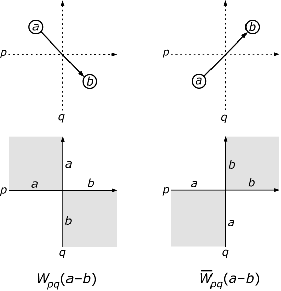
Figure 1: The two kinds of chiral Potts model Boltzmann weights $W_{pq}(a-b)$ and $\overline{W}_{pq}(a-b)$. The handedness is indicated by arrows between the spins of values $a$ and $b$. Also given are the oriented lines on which rapidities $p$ and $q$ live. Row two gives the equivalent checkerboard vertex model representation.

The first thing to be decided was a proper notation for the Boltzmann weights. We clearly needed to incorporate Baxter’s $Z$-invariance [23, 24], but we decided to use notations from [25], see figure 1. In analogy with relativistic scattering theory we decided to call the spectral variables $p,q,r$ rapidities and to put arrows on the rapidity lines. The chirality of the interactions between spins, $a,b,\cdots,$ is indicated by arrows. The Potts nature means that the weights depend on differences $a-b$ mod $N$. Not to give the same figures every time, I have here also given the equivalent checkerboard vertex model representation, representing the star-triangle equations as in figure 2.

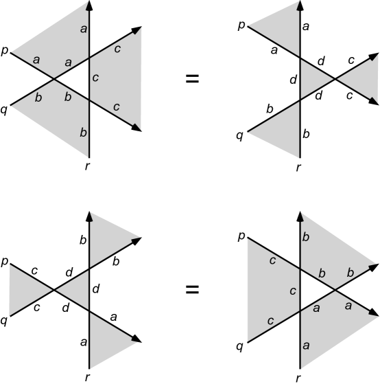
Figure 2: The star-triangle equations represented as checkerboard Yang–Baxter equations. For the chiral Potts model both equations (interchanging grey and white colorings of the faces) are equivalent.

For several days the three of us made attempts to generalize the conjectured product form (21) for the self-dual case. At some point I proposed to look at the Ising model and to write the theta functions of the differences of $p$ and $q$ as sums of products of functions of $p$ and $q$ separately. We could use either Onsager’s paper [26] or our two papers [24, 25]. Baxter and Au-Yang thought that I was crazy to guess a product from a single factor and I was to finish the calculation I was doing. The next day we went for an outing in Tidbinbilla, but the morning after Baxter came up with the desired product forms [27],

$${W_{pq}(n)\over W_{pq}(0)}=\prod_{j=1}^{n}\,{d_{p}b_{q}-a_{p}c_{q}\omega^{j}\over b_{p}d_{q}-c_{p}a_{q}\omega^{j}},\qquad{{\overline{W}}_{pq}(n)\over{\overline{W}}_{pq}(0)}=\prod_{j=1}^{n}\,{\omega a_{p}d_{q}-d_{p}a_{q}\omega^{j}\over c_{p}b_{q}-b_{p}c_{q}\omega^{j}}.$$ (22)

Periodicity mod $N$, $W_{pq}(n+N)=W_{pq}(n)$, ${\overline{W}}_{pq}(n+N)={\overline{W}}_{pq}(n)$, led to the chiral Potts curve condition for the rapidities $x_{p}=(a_{p},b_{p},c_{p},d_{p})$,

$$a_{p}^{\,N}+k^{\prime}b_{p}^{\,N}=k\,d_{p}^{\,N},\quad k^{\prime}a_{p}^{\,N}+b_{p}^{\,N}=k\,c_{p}^{\,N},\quad k^{2}+k^{\prime}{}^{2}=1,$$ (23)

using a suitable normalization. We did extensive checking using Fortran on the new little Macintosh computers at Australian National University and the scalar factor $R$ in the star-triangle equation was guessed also from Ising and checked by Fortran. Our letter [27] contains many more results, and we obtained a proof that the star-triangle equations are satisfied using recurrences based on variations of (2). This proof was published a few years later in the appendix of [28].

2.4 Free energy, order parameters and functional equation

During these six weeks in Canberra, I made a brief visit to Melbourne which was also very significant, because Paul Pearce gave me a copy of a preprint by Bazhanov and Reshetikhin. This preprint contained a cubic functional relation, that was omitted in the published version [29]. As the Onsager algebra [19] and the paper of von Gehlen and Rittenberg [15] indicated that the chiral Potts model is a cyclic version of quantum sl(2), we conjectured that chiral Potts would have a similar functional relation. Barry McCoy thus made his students Tang and Albertini solve the eigenvalue problem for small systems so that soon numerical support for our conjecture would be available.

In the meantime, Baxter obtained the first free-energy result by the “399th” method [30] to solve the Ising model and he found the specific heat exponent to be $\alpha=1-2/N$ for the two-dimensional classical case [31].

The small chain results for the von Gehlen–Rittenberg special case were particularly simple and McCoy coined the term ‘superintegrable’ for this case with extra Onsager-algebra integrability, as several concepts were being ‘supered’ by our high-energy colleagues in Stony Brook. Therefore, as I had some traveling to do, I wrote a couple of self-submitting batch jobs in SMP on the three Ridge Unix computers of the Institute for Theoretical Physics that gave us iteratively the ground state energy of the superintegrable chain in the commensurate phase for chains of considerable length, leading to long series expansions for $N=3$, 4, 5 and general $N$. At some higher orders I had to work around multiplication errors in the SMP program.

Also our earlier labor doing series expansions trying to get Painlevé-type results paid off: One day McCoy told us to look again at the paper by Howes, Kadanoff and den Nijs [32], as they had conjectured a particularly simple result for the order parameter of the 3-state superintegrable quantum chain in the ordered ground state, namely $(1-\lambda^{2})^{1/9}$ [32, eq. (3.13)]. They stated that they had done a series expansion that reproduced this conjecture to thirteenth order! Soon we obtained the leading terms in the expansion of the order parameters for general $N$, so that we could generalize their conjecture as

$$\langle\mathbf{Z}_{0}^{\,k}\rangle=(1-\lambda^{2})^{k(N-k)/2N^{2}}.$$ (24)

Invoking Baxter’s $Z$-invariance [23], this result should apply also to the ordered phase of the full integrable chiral Potts model, both for the one-dimensional quantum chain and the two-dimensional classical case.

However, this was based on only very few terms. Luckily, just walking by, I noted a preprint of Henkel and Lacki [33] on the very top of a pile of discarded preprints in one of the garbage bins of the ITP. This gave further confirmation, as Henkel and Lacki had expanded the sum of the order parameters to one more order than we had done. Unfortunately for them, for $N\geq 4$ this sum does not have the binomial form that it has for $N=2$ and 3. Our conjecture was submitted May 1988 in a paper with several other results [35].

Early October 1988 we received a preprint of Baxter [36] in which he solved several properties of the superintegrable case by the inversion relation. About a week later we submitted our paper [37] with our cubic functional equation that had been verified by Albertini for several chain lengths using Fortran. As a result, we found that there had to exist a commensurate-incommensurate phase transition in the superintegrable 3-state chain [37] for $\lambda<1$, so that the conjectured phase diagram in [32, figure 2] with a Lifshitz point at $\lambda=1$ is not quite correct.

At the Taniguchi conference, October 1988, Miwa made me present a detailed proof that the weights (22) satisfy the star-triangle equation. Each time I had filled his high-tech whiteboard he printed a copy of what I had written. A more elaborate paper appears in the proceedings [28], with the proof given in the appendix. McCoy presented details [38] about the appearance of the incommensurate phase in the 3-state superintegrable quantum chain. Multi-particle excitations were also studied to estimate size of the incommensurate phase [39].

2.5 Representation theoretical understanding, outlook and some prehistory

There were many further developments, especially the representation theory explanation of Bazhanov and Stroganov, valid for odd $N$ [40, 41], and an alternative approach valid for all $N$ [42]. The difference of these two approaches is discussed in the next section. These two works made the relation with cyclic representations of quantum groups as described later by De Concini and Kac [43] explicit, confirming our earlier thoughts on it.

There should be some models that have rapidities on higher-genus curves other than the one of chiral Potts. Martins [44] claims to have found a model parametrized by a K3 surface recently and it would be interesting to investigate this further.

To conclude this section, we should mention some early works of Krichever and Korepanov, of which we were not aware until some time in 1993 when we received some copies in Russian in the mail. In [45, 46] Krichever proved his Theorem 1 stating that generically the genus of the curve coming from vacuum vectors of an $N$-state model related to the six-vertex model had to be $(N-1)^{2}$, but he only worked out the case $N=2$ in detail. Korepanov followed this up studying the cases $N=3$ and greater [47], discovering thus the Boltzmann weight of some $\tau_{2}$ model, in agreement with Krichever’s theorem and with [45, equation (13)], [46, equation (10)]. This way, though unknown outside the Soviet Union for many years, Korepanov gave the first explicit demonstration of a solution of the quantum Yang–Baxter equation with a higher-genus parametrization, several months before the discovery of the integrable chiral Potts model.

However, Korepanov did not discover the integrable chiral Potts model, nor did he construct the $R$-matrix intertwining two cyclic representations. That construction had to wait until [40, 41]. Only with the complete construction does one know that both the horizontal and vertical transfer matrices of the $\tau_{2}$ model form commuting families with one set of spectral parameters (rapidities) taken from the high-genus curve and the other set from the genus-zero curve of the six-vertex model. Until [40, 41] the meaning of Korepanov’s discovery was veiled.

Finally, in the introduction of our recent paper [48] one can find some other references related to parafermions that are of historical interest, including papers on generalized Clifford algebras.

3 Part 2: Odd or Even

3.1 Ising case $N=2$: Onsager algebra and Jordan–Wigner transformation

When $N=2$, the integrable chiral Potts model becomes the Ising model. The chiral Potts spin-chain Hamiltonian (9) reduces to

$$\mathcal{H}=\sum_{j=1}^{L}\big{(}\alpha_{1}\mathbf{Z}_{j}\mathbf{Z}_{j+1}+\bar{\alpha}_{1}\mathbf{X}_{j}\big{)}=-\sum_{j=1}^{L}\big{(}J\sigma^{z}_{j}\sigma^{z}_{j+1}+B\sigma^{x}_{j}\big{)},$$ (25)

identifying $\mathbf{X}=\sigma^{x}$ and $\mathbf{Z}=\sigma^{z}$ as Pauli matrices, and $\alpha_{1}=-J$, $\bar{\alpha}_{1}=-B$. This is the transverse-field Ising chain Hamiltonian, now so popular in quantum information circles. As said before, the connection with the Ising model for $N=2$ has been very important for us to find the high-genus solutions of the star-triangle equations [27, 28].

In the Ising case of spin-${1\over 2}$, the spin operators have mixed commutation relations: commuting if at different sites, but anticommuting at the same site. This was first addressed in the Ising model context by Bruria Kaufman [49], who introduced the Clifford algebra spinors,

$$\Gamma_{2j-1}=\mathbf{X}_{1}\mathbf{X}_{2}\cdots\mathbf{X}_{j-1}\mathbf{Z}_{j},\quad\Gamma_{2j}=\mathrm{i}\mathbf{X}_{1}\mathbf{X}_{2}\cdots\mathbf{X}_{j}\mathbf{Z}_{j},\quad\Gamma_{m}\Gamma_{n}+\Gamma_{n}\Gamma_{m}=2\delta_{mn}.$$ (26)

A generalization to spin-${1\over 2}$ XXZ models at roots of unity was introduced by Deguchi, Fabricius and McCoy [50]. Nishino and Deguchi [51] found a further generalization applicable to the superintegrable $\tau_{2}$-model when $N$ is odd, as required in [41]. This was followed by a series of papers on the superintegrable $\tau_{2}$ and chiral Potts models [52, 53, 54, 55, 56, 57, 58, 59] for general $N$ using [42]. In these papers we constructed the eigenvectors in the ground state sector and the order parameters using a generalized Jordan–Wigner transform.

In these superintegrable models there is additional sl(2) loop group symmetry, supporting representations of the Onsager algebra [19, 26],

$$[A_{j},A_{k}]=4G_{j-k},\qquad[G_{m},A_{l}]=2A_{l+m}-2A_{l-m},\qquad[G_{j},G_{k}]=0,$$ (27)

but with a more complicated closure relation than in the Ising model. It should be noted that von Gehlen and Rittenberg [15] had already constructed the superintegrable chiral Potts quantum chain in 1985, using the Dolan–Grady criterion [18, 19, 61],

$$\mathcal{H}=A_{0}+\lambda A_{1},\quad [A_{0},[A_{0},[A_{0},A_{1}]]]=16[A_{0},A_{1}],$$ (28)

$$[A_{1},[A_{1},[A_{1},A_{0}]]]=16[A_{1},A_{0}].$$

which is a kind of Serre relation implying the existence of the Onsager algebra.

3.2 Bazhanov–Stroganov construction

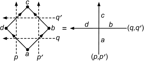
Figure 3: Square of four chiral Potts weights (22) represented by four oriented solid lines connecting the Potts spins $a$, $b$, $c$ and $d$. The four rapidity lines are drawn dashed. This is equivalent to a vertex model with the spins living on line pieces.

A quantum group construction of the integrable chiral Potts model has first been given by Bazhanov and Stroganov [41] for odd $N$, starting from an R-matrix of the six-vertex model, the intertwiner of two highest-weight spin-$1\over 2$ representations. They constructed next the intertwiner of a spin-$1\over 2$ and a cyclic representation ($\tau_{2}$-model weights). Finally, the square of four chiral Potts weights as given in [27] and figure 3 was shown to intertwine two cyclic representations.

The more general the six-vertex R-matrix is chosen, the more easy it is to arrive at the chiral Potts model. Korepanov [47] had chosen $R^{00}_{00}=R^{11}_{11}$, $R^{01}_{01}=R^{10}_{10}$ and $R^{10}_{01}=R^{01}_{10}$. Bazhanov and Stroganov [41] made a special gauge choice with $R^{10}_{01}\neq R^{01}_{10}$, whereas [42] also ended up with $R^{01}_{01}\neq R^{10}_{10}$, see [60, equation (1.7)] for the comparison.

3.3 Baxter–Bazhanov–Perk construction

Figure 4: Star of four chiral Potts weights (22) represented by four oriented solid lines connecting the Potts spins $a$, $b$, $c$, $d$ and $e$. Summing over the value of $e$ this becomes the IRF model weight on the right.

In order to get a construction valid for all $N$, Baxter, Bazhanov and Perk [42] started in the opposite direction with a star of chiral Potts model weights as in figure 4, with Boltzmann weights defined by (22) and figure 1. Summing out the central spin gives an Interaction-Round-a-Face (IRF) model weight $U_{pp^{\prime}qq^{\prime}}(a,b,c,d)$, which can also be viewed as a vertex model weight using the well-known map assigning spin differences mod $N$ to the line pieces.

If one now chooses $(x_{q^{\prime}},y_{q^{\prime}},\mu_{q^{\prime}})=(y^{\vphantom{y}}_{q},\omega^{2}x^{\vphantom{y}}_{q},\mu_{q}^{-1})$, then $U_{pp^{\prime}qq^{\prime}}(a,b,c,d)=0$ for $0\leq a-d\leq 1$ and $2\leq b-c\leq N-1$, so that $U$ is triangular and the leading block is the R-matrix of a $\tau_{2}$ model. If one also chooses $(x_{p^{\prime}},y_{p^{\prime}},\mu_{p^{\prime}})=(y^{\vphantom{y}}_{p},\omega^{2}x^{\vphantom{y}}_{p},\mu_{p}^{-1})$, then also $U_{pp^{\prime}qq^{\prime}}(a,b,c,d)=0$ for $0\leq d-c\leq 1$ and $2\leq a-b\leq N-1$, and we receive a six-vertex R-matrix.

We consider from now on the superintegrable case $(x_{p^{\prime}},y_{p^{\prime}},\mu_{p^{\prime}})=(y^{\vphantom{y}}_{p},x^{\vphantom{y}}_{p},\mu_{p}^{-1})$. Then, dropping some overall factors we can write the $2^{2}\!\times\!2^{2}$ R-matrix as

$$R(x,y)=\pmatrix{1-{\displaystyle{x\over y}}\omega^{-1}&0&0&0\cr 0&1-{\displaystyle{x\over y}}&{\displaystyle{x\over y}}(1-\omega^{-1})&0\cr 0&1-\omega^{-1}&(1-{\displaystyle{x\over y}})\omega^{-1}&0\cr 0&0&0&1-{\displaystyle{x\over y}}\omega^{-1}}$$ (29)

and the $2N\!\times\!2N$ $\tau_{2}$ R-matrix as

$$U(x)=\pmatrix{U_{00}&U_{01}\cr U_{10}&U_{11}}=\pmatrix{{\bf 1}-\omega x\mathbf{Z}&-\omega x({\bf 1}-\mathbf{Z})\mathbf{X}\cr\mathbf{X}^{-1}({\bf 1}-\mathbf{Z})&\omega(\mathbf{Z}-x\mathbf{1})}.$$ (30)

Here $x$ and $y$ are genus-0 rapidities of the six-vertex model, $\mathbf{X}$ and $\mathbf{Z}$ are the $N\!\times\!N$ matrices defined before.

Note that $R(x,y)$ is a linear combination of only 1, $\textstyle{x\over y}$, $\omega^{-1}$ and $\textstyle{x\over y}\omega^{-1}$. This makes that choice particularly amenable for further analysis.

3.4 The monodromy matrix and its expansion coefficients

We can string $L$ $\tau_{2}$-model R-matrices together to form a monodromy matrix. Writing

$${\cal L}(x)=\pmatrix{{\cal L}_{00}&{\cal L}_{01}\cr{\cal L}_{10}&{\cal L}_{11}}=\pmatrix{\mbox{\myss A}(x)&\mbox{\myss B}(x)\cr\mbox{\myss C}(x)&\mbox{\myss D}(x)},$$ (31)

following notations of the Faddeev school [62]. Then two such monodromy matrices ${\cal L}(x)$ and ${\cal L}(y)$ satisfy a Yang–Baxter equation with the six-vertex R-matrix. This is so, both for the finite-dimensional case with $\omega$ and the infinite-dimensional case with generic $q$ that we shall introduce later.

The monodromy matrix ${\cal L}(x)$ is a polynomial in $x$ of degree $L$. So, we write

$$\mbox{\myss A}(x)=\sum_{l=0}^{L}\mathbf{A}_{l}x^{l},\quad\mbox{\myss B}(x)=\sum_{l=1}^{L}\mathbf{B}_{l}x^{l},\quad\mbox{\myss C}(x)=\sum_{l=0}^{L-1}\mathbf{C}_{l}x^{l},\quad\mbox{\myss D}(x)=\sum_{l=0}^{L}\mathbf{D}_{l}x^{l}.$$ (32)

In each of these four series all coefficients commute. It is easy to work out some of these coefficients explicitly [52, 56]

$$\mathbf{A}_{0}=\mathbf{D}_{L}=\mathbf{1},\qquad\mathbf{A}_{L}=\mathbf{D}_{0}\,\omega^{-L}=\prod_{j=1}^{L}\mathbf{Z}_{j},\qquad\mathbf{C}_{L}=\mathbf{B}_{0}=0,$$

$$\overline{\mathbf{B}}_{L}={\mathbf{B}_{L}\over 1-\omega}=\sum_{j=1}^{L}\bigg{(}\prod_{m=1}^{j-1}\mathbf{Z}_{m}\!\bigg{)}{\hbox{\mbox{\bfra f}}}_{j},\qquad\overline{\mathbf{C}}_{0}={\mathbf{C}_{0}\over 1-\omega}=\sum_{j=1}^{L}\bigg{(}\prod_{m=1}^{j-1}(\omega\mathbf{Z}_{m})\!\bigg{)}{\hbox{\mbox{\bfra e}}}_{j},$$

$$\overline{\mathbf{B}}_{1}={\mathbf{B}_{1}\over 1-\omega}=\sum_{j=1}^{L}{{\mbox{\bfra f}}}_{j}\prod_{m=j+1}^{L}(\omega\mathbf{Z}_{m}),\quad\overline{\mathbf{C}}_{L-1}={\mathbf{C}_{L-1}\over 1-\omega}=\sum_{j=1}^{L}{{\mbox{\bfra e}}}_{j}\prod_{m=j+1}^{L}\mathbf{Z}_{m}.$$ (33)

We note that some of these look like coproducts. The ${\mbox{\bfra e}}_{j}$ and ${\mbox{\bfra f}}_{j}$ are defined by having

$${\mbox{\bfra e}}={\mathbf{X}^{-1}({\bf 1}-\mathbf{Z})\over 1-\omega}\qquad\hbox{and}\qquad{\mbox{\bfra f}}={({\bf 1}-\mathbf{Z})\mathbf{X}\over 1-\omega}$$ (34)

acting only on position $j$.

The eigenstates of the superintegrable $\tau_{2}$ model are highly degenerate and we can define creation and annihilation operators within each sector by

$$\mathbf{x}^{+}_{0,Q}=\mathbf{C}^{(N+Q)}_{0}\mathbf{B}^{(Q)}_{1},\quad\mathbf{x}^{-}_{1,Q}=\mathbf{C}^{(Q)}_{0}\mathbf{B}^{(N+Q)}_{1},\quad(Q=0,\cdots,N-1).$$ (35)

Here we defined

$$\mathbf{B}^{(n)}_{1}={\mathbf{B}^{\;n}_{1}\over(n)_{\omega}!},\qquad\mathbf{C}^{(n)}_{0}={\mathbf{C}^{\;n}_{0}\over(n)_{\omega}!},$$ (36)

using the $q$-factorial and $q$-integers

$$(n)_{q}!=(n)_{q}(n-1)_{q}\cdots(1)_{q},\qquad(n)_{q}={1-q^{n}\over 1-q}=1+q+q^{2}+\cdots+q^{n-1},$$ (37)

with $q=\omega$.

For each $Q$ between 0 and $N-1$, $\mathbf{x}^{+}_{0,Q}$ and $\mathbf{x}^{-}_{1,Q}$ generate an sl(2) (sub)algebra provided the Serre relations

$$[\mathbf{x}^{+}_{0,Q},[\mathbf{x}^{+}_{0,Q},[\mathbf{x}^{+}_{0,Q},\mathbf{x}^{-}_{1,Q}]\,]\,]=0,\quad[\mathbf{x}^{-}_{1,Q},[\mathbf{x}^{-}_{1,Q},[\mathbf{x}^{-}_{1,Q},\mathbf{x}^{+}_{0,Q}]\,]\,]=0,$$ (38)

hold.

3.5 Infinite-dimensional representation

In order to properly define all this, it will be important to analytically continue in $\omega$. But then we need the infinite-dimensional representation

$$\mathbf{X}_{q}\equiv\pmatrix{0&0&0&\ldots&0&0&\ldots\cr 1&0&0&\ldots&0&0&\ldots\cr 0&1&0&\ldots&0&0&\ldots\cr\vdots&\vdots&\vdots&\ddots&\vdots&\vdots\cr 0&0&0&\ldots&0&0&\ldots\cr 0&0&0&\ldots&1&0&\ldots\cr\vdots&\vdots&\vdots&&\vdots&\vdots\cr},\qquad\mathbf{Z}_{q}\equiv\pmatrix{1&0&0&\ldots&0&0&\ldots\cr 0&q&0&\ldots&0&0&\ldots\cr 0&0&q^{2}&\ldots&0&0&\ldots\cr\vdots&\vdots&\vdots&\ddots&\vdots&\vdots\cr 0&0&0&\ldots&\hskip-5.0ptq^{N-2}\hskip-5.0pt&0&\ldots\cr 0&0&0&\ldots&0&\hskip-20.0ptq^{N-1}\hskip-20.0pt&\ldots\cr\vdots&\vdots&\vdots&&\vdots&\vdots\cr},$$ (39)

satisfying $\mathbf{Z}_{q}\mathbf{X}_{q}=q\mathbf{X}_{q}\mathbf{Z}_{q}$.

Also, we really only need

$${\mbox{\bfra e}}_{q}={\mathbf{X}_{q}^{-1}({\bf 1}-\mathbf{Z}_{q})\over 1-q}\qquad\hbox{and}\qquad\hbox{\mbox{\bfra f}}_{q}={({\bf 1}-\mathbf{Z}_{q})\mathbf{X}_{q}\over 1-q}$$ (40)

so that the extra 1, present in the finite-dimensional case in the upper-right corner of $\mathbf{X}$ and making $\mathbf{X}$ a cyclic matrix, cancels out.

Using the $q$-integers (37), we can write

$${\mbox{\bfra e}}_{q}\equiv\pmatrix{0&\!\!\!(1)_{q}\!\!\!&0&\ldots&0&0&\ldots\cr 0&0&\!\!\!(2)_{q}\!\!\!&\ldots&0&0&\ldots\cr 0&0&0&\ldots&0&0&\ldots\cr\vdots&\vdots&\vdots&\ddots&\vdots&\vdots\cr 0&0&0&\ldots&0&\!\!\!(n)_{q}\!\!\!&\ldots\cr 0&0&0&\ldots&0&0&\ldots\cr\vdots&\vdots&\vdots&&\vdots&\vdots\cr},\quad{\mbox{\bfra f}}_{q}\equiv\pmatrix{0&0&0&\ldots&0&0&\ldots\cr\!\!(1)_{q}\!\!\!&0&0&\ldots&0&0&\ldots\cr 0&\!\!\!(2)_{q}\!\!\!&0&\ldots&0&0&\ldots\cr\vdots&\vdots&\vdots&\ddots&\vdots&\vdots\cr 0&0&0&\ldots&0&0&\ldots\cr 0&0&0&\ldots&\!\!\!(n)_{q}\!\!\!&0&\ldots\cr\vdots&\vdots&\vdots&&\vdots&\vdots\cr},$$ (41)

or

$$({\mbox{\bfra e}}_{q})_{kl}=(k)_{q}\,\delta_{k+1,l},\qquad({\mbox{\bfra f}}_{q})_{kl}=(l)_{q}\,\delta_{k,l+1},\qquad(\mathbf{Z}_{q})_{kl}=q^{k-1}\,\delta_{k,l}.$$ (42)

Also,

$${\mbox{\bfra e}}_{q}{\mbox{\bfra f}}_{q}-q\,{\mbox{\bfra f}}_{q}{\mbox{\bfra e}}_{q}={1-q\mathbf{Z}_{q}^{\;2}\over 1-q},\qquad{\mbox{\bfra e}}_{q}\mathbf{Z}_{q}=q\,\mathbf{Z}_{q}{\mbox{\bfra e}}_{q},\qquad\mathbf{Z}_{q}{\mbox{\bfra f}}_{q}=q\,{\mbox{\bfra f}}_{q}\mathbf{Z}_{q}.$$ (43)

When $q$ is an $N$th root of unity, $(N)_{q}=0$ and the first $N\!\times\!N$ block decouples from the rest, making ${\mbox{\bfra e}}_{q}$, ${\mbox{\bfra f}}_{q}$ and $\mathbf{Z}_{q}$ block diagonal. Said differently, replacing $q$ by $\omega$, we only need to keep the first $N\!\times\!N$ block.

3.6 Commutators and $q$-commutators

Replacing $\omega$ by generic $q$ in (29), the six-vertex R-matrix with the special choice of the gauge rapidities in the Yang–Baxter equation (see [11, equation (20)]) becomes

$$R(x,y)=\pmatrix{1-{\displaystyle{x\over y}}q^{-1}&0&0&0\cr 0&1-{\displaystyle{x\over y}}&{\displaystyle{x\over y}}(1-q^{-1})&0\cr 0&1-q^{-1}&(1-{\displaystyle{x\over y}})q^{-1}&0\cr 0&0&0&1-{\displaystyle{x\over y}}q^{-1}}.$$ (44)

We can now take any monodromy matrix (31) associated with it and write the Yang–Baxter equation out in terms of the A, B, C, D [62]. Then we get the following sixteen equations:

$$[\mbox{\myss A}(x),\mbox{\myss A}(y)]=[\mbox{\myss B}(x),\mbox{\myss B}(y)]=[\mbox{\myss C}(x),\mbox{\myss C}(y)]=[\mbox{\myss D}(x),\mbox{\myss D}(y)]=0,$$ (45)

$$(1-\textstyle{x\over y}{q^{-1}})\mbox{\myss B}(x)\mbox{\myss A}(y)=\textstyle{x\over y}(1-{q^{-1}})\mbox{\myss B}(y)\mbox{\myss A}(x)+(1-\textstyle{x\over y}){q^{-1}}\mbox{\myss A}(y)\mbox{\myss B}(x),$$

$$(1-\textstyle{x\over y}{q^{-1}})\mbox{\myss A}(x)\mbox{\myss B}(y)=(1-\textstyle{x\over y})\mbox{\myss B}(y)\mbox{\myss A}(x)+(1-{q^{-1}})\mbox{\myss A}(y)\mbox{\myss B}(x),$$ (46)

$$\textstyle{x\over y}(1-{q^{-1}})\mbox{\myss C}(x)\mbox{\myss A}(y)+(1-\textstyle{x\over y})\mbox{\myss A}(x)\mbox{\myss C}(y)=(1-\textstyle{x\over y}{q^{-1}})\mbox{\myss C}(y)\mbox{\myss A}(x),$$

$$(1-\textstyle{x\over y}){q^{-1}}\mbox{\myss C}(x)\mbox{\myss A}(y)+(1-{q^{-1}})\mbox{\myss A}(x)\mbox{\myss C}(y)=(1-\textstyle{x\over y}{q^{-1}})\mbox{\myss A}(y)\mbox{\myss C}(x),$$ (47)

$$\textstyle{x\over y}(1-{q^{-1}})\mbox{\myss D}(x)\mbox{\myss B}(y)+(1-\textstyle{x\over y})\mbox{\myss B}(x)\mbox{\myss D}(y)=(1-\textstyle{x\over y}{q^{-1}})\mbox{\myss D}(y)\mbox{\myss B}(x),$$

$$(1-\textstyle{x\over y}){q^{-1}}\mbox{\myss D}(x)\mbox{\myss B}(y)+(1-{q^{-1}})\mbox{\myss B}(x)\mbox{\myss D}(y)=(1-\textstyle{x\over y}{q^{-1}})\mbox{\myss B}(y)\mbox{\myss D}(x),$$ (48)

$$(1-\textstyle{x\over y}{q^{-1}})\mbox{\myss D}(x)\mbox{\myss C}(y)=\textstyle{x\over y}(1-{q^{-1}})\mbox{\myss D}(y)\mbox{\myss C}(x)+(1-\textstyle{x\over y}){q^{-1}}\mbox{\myss C}(y)\mbox{\myss D}(x),$$

$$(1-\textstyle{x\over y}{q^{-1}})\mbox{\myss C}(x)\mbox{\myss D}(y)=(1-\textstyle{x\over y})\mbox{\myss D}(y)\mbox{\myss C}(x)+(1-{q^{-1}})\mbox{\myss C}(y)\mbox{\myss D}(x),$$ (49)

$$\textstyle{x\over y}(1-{q^{-1}})\mbox{\myss D}(x)\mbox{\myss A}(y)+(1-\textstyle{x\over y})\mbox{\myss B}(x)\mbox{\myss C}(y)$$

$$=\textstyle{x\over y}(1-{q^{-1}})\mbox{\myss D}(y)\mbox{\myss A}(x)+(1-\textstyle{x\over y}){q^{-1}}\mbox{\myss C}(y)\mbox{\myss B}(x),$$

$$\textstyle{x\over y}(1-{q^{-1}})\mbox{\myss C}(x)\mbox{\myss B}(y)+(1-\textstyle{x\over y})\mbox{\myss A}(x)\mbox{\myss D}(y)$$

$$=(1-\textstyle{x\over y})\mbox{\myss D}(y)\mbox{\myss A}(x)+(1-{q^{-1}})\mbox{\myss C}(y)\mbox{\myss B}(x),$$ (50)

$$(1-\textstyle{x\over y}){q^{-1}}\mbox{\myss D}(x)\mbox{\myss A}(y)+(1-{q^{-1}})\mbox{\myss B}(x)\mbox{\myss C}(y)$$

$$=\textstyle{x\over y}(1-{q^{-1}})\mbox{\myss B}(y)\mbox{\myss C}(x)+(1-\textstyle{x\over y}){q^{-1}}\mbox{\myss A}(y)\mbox{\myss D}(x),$$

$$(1-\textstyle{x\over y}){q^{-1}}\mbox{\myss C}(x)\mbox{\myss B}(y)+(1-{q^{-1}})\mbox{\myss A}(x)\mbox{\myss D}(y)$$

$$=(1-\textstyle{x\over y})\mbox{\myss B}(y)\mbox{\myss C}(x)+(1-{q^{-1}})\mbox{\myss A}(y)\mbox{\myss D}(x).$$ (51)

Note that we have a symmetry under the simultaneous replacements $\mbox{\myss A}\leftrightarrow\mbox{\myss C}$ and $\mbox{\myss B}\leftrightarrow\mbox{\myss D}$, as (46) $\leftrightarrow$ (49) and (47) $\leftrightarrow$ (48); if we replace $x\leftrightarrow y$ then also (50) $\leftrightarrow$ (51).

At this point we stress that the special asymmetric gauge of $R(x,y)$ causes all coefficients to be linear combinations of only 1, $\textstyle{x\over y}$, $\omega^{-1}$ and $\textstyle{x\over y}\omega^{-1}$. This we could have because we chose to use [42] rather than [41]. It makes expansions in powers of $x$ and $y$ particularly attractive.

Of course, the 16 equations (45) through (51) with $x\leftrightarrow y$ are also valid. Using all 32 equations we find the following 10 commutator equations and 6 $q$-commutator equations:

$$[\mbox{\myss A}(x),\mbox{\myss A}(y)]=[\mbox{\myss B}(x),\mbox{\myss B}(y)]=[\mbox{\myss C}(x),\mbox{\myss C}(y)]=[\mbox{\myss D}(x),\mbox{\myss D}(y)]=0,$$

$$[\mbox{\myss A}(x),\mbox{\myss B}(y)]=[\mbox{\myss A}(y),\mbox{\myss B}(x)],\quad[\mbox{\myss C}(x),\mbox{\myss D}(y)]=[\mbox{\myss C}(y),\mbox{\myss D}(x)],$$

$$[\mbox{\myss A}(x),\mbox{\myss D}(y)]=[\mbox{\myss A}(y),\mbox{\myss D}(x)],$$

$$y[\mbox{\myss A}(x),\mbox{\myss C}(y)]=x[\mbox{\myss A}(y),\mbox{\myss C}(x)],\quad y[\mbox{\myss B}(x),\mbox{\myss D}(y)]=x[\mbox{\myss B}(y),\mbox{\myss D}(x)],$$

$$y[\mbox{\myss A}(x),\mbox{\myss D}(y)]+y[\mbox{\myss B}(x),\mbox{\myss C}(y)]=x[\mbox{\myss A}(y),\mbox{\myss D}(x)]+x[\mbox{\myss B}(y),\mbox{\myss C}(x)],$$

$$[\mbox{\myss C}(x),\mbox{\myss A}(y)]_{q}=[\mbox{\myss C}(y),\mbox{\myss A}(x)]_{q}\,,\quad[\mbox{\myss D}(x),\mbox{\myss B}(y)]_{q}=[\mbox{\myss D}(y),\mbox{\myss B}(x)]_{q}\,,$$

$$[\mbox{\myss D}(x),\mbox{\myss A}(y)]_{q}+[\mbox{\myss C}(x),\mbox{\myss B}(y)]_{q}=[\mbox{\myss D}(y),\mbox{\myss A}(x)]_{q}+[\mbox{\myss C}(y),\mbox{\myss B}(x)]_{q}\,,$$

$$x[\mbox{\myss A}(x),\mbox{\myss B}(y)]_{q}=y[\mbox{\myss A}(y),\mbox{\myss B}(x)]_{q}\,,\quad x[\mbox{\myss C}(x),\mbox{\myss D}(y)]_{q}=y[\mbox{\myss C}(y),\mbox{\myss D}(x)]_{q}\,,$$

$$x[\mbox{\myss C}(x),\mbox{\myss B}(y)]_{q}=y[\mbox{\myss C}(y),\mbox{\myss B}(x)]_{q}\,,$$ (52)

where $[\mbox{\myss X},\mbox{\myss Y}]_{q}\equiv\mbox{\myss X}\mbox{\myss Y}-q\mbox{\myss Y}\mbox{\myss X}\;.$ This structure is a consequence of the special choice (44).

3.7 Quantum group and coproducts

The notion of quantum group came about after many years of progress by many people. To me two papers by Zamolodchikov and Zamolodchikov [63] and by Berg et al. [64] were very significant, as they gave me the idea that somehow R-matrices are associated with groups. At a conference in Kyoto, May 1981, Jimbo asked me how the models that I had presented in my talk [65] fit into a larger classification. I answered him that I believed that they should be classified with the first series of Dynkin diagrams.

Sklyanin seems to be the first to have suggested that the correct mathematical framework associated with R-matrices is Hopf algebras, in a one page note in Russian [66] on his two earlier works on quantum algebra structures [67, 68]. The works of Drinfeld [69] and Jimbo [70, 71] describe a lot of the structure of what now is called quantum groups, a term first coined by Drinfeld [72]. Here I prefer to use Jimbo’s review [73], as it also addresses the chiral Potts model, albeit only for $N$ odd, even though the case $N$ even can be dealt with [60] also.

To make contact with the quantum group ${\rm U}_{q}(\widehat{\hbox{\mbox{\bfra s}l}}_{2})$, we assume $q\to\pm\omega^{1/2}$, defining a proper limiting process where it is needed. We define the generators to be

$$e_{0}=q\mbox{\myss Z}_{q}^{\,-1}\hbox{\mbox{\bfra f}}_{q^{2}}^{\vphantom{y}}={\mbox{\myss Z}_{q}^{\vphantom{y}}-\mbox{\myss Z}_{q}^{\,-1}\over q-q^{-1}}\mathbf{X},\qquad e_{1}=f_{0}\lambda^{-1},$$

$$f_{0}=-q\hbox{\mbox{\bfra e}}_{q^{2}}^{\vphantom{y}}\mbox{\myss Z}_{q}^{\,-1}=-\mathbf{X}^{\rm T}{\mbox{\myss Z}_{q}^{\vphantom{y}}-\mbox{\myss Z}_{q}^{\,-1}\over q-q^{-1}},\qquad f_{1}=e_{0}\lambda,$$

$$k_{0}=q\mbox{\myss Z}_{q}^{\,2},\qquad k_{1}=k_{0}^{-1},$$ (53)

where $\lambda$ is a complex parameter and ${\mbox{\bfra e}}_{q^{2}}$ and ${\mbox{\bfra f}}_{q^{2}}$ are defined in (40). It is easily verified that these generators satisfy the required relations

$$e_{i}f_{j}-f_{j}e_{i}=\delta_{ij}{k_{i}^{\vphantom{y}}-k_{i}^{\,-1}\over q-q^{-1}},$$ (54)

$${e_{i}^{\,n}\over[n]_{q}!}\hbox{ and }\;{f_{i}^{\,n}\over[n]_{q}!}\hbox{ Laurent polynomials in }q,$$ (55)

$$k_{i}^{\,1/2}e_{i}^{\vphantom{y}}=qe_{i}^{\vphantom{y}}k_{i}^{\,1/2},\qquad k_{i}^{\,1/2}e_{j}^{\vphantom{y}}=q^{-1}e_{j}^{\vphantom{y}}k_{i}^{\,1/2},$$

$$k_{i}^{\,1/2}f_{i}^{\vphantom{y}}=q^{-1}f_{i}^{\vphantom{y}}k_{i}^{\,1/2},\quad k_{i}^{\,1/2}f_{j}^{\vphantom{y}}=qf_{j}^{\vphantom{y}}k_{i}^{\,1/2},$$ (56)

$$e_{i}^{\,3}e_{j}^{\vphantom{y}}\,-[3]_{q}\,e_{i}^{\,2}e_{j}^{\vphantom{y}}e_{i}^{\vphantom{y}}\,+[3]_{q}\,e_{i}^{\vphantom{y}}e_{j}^{\vphantom{y}}e_{i}^{\,2}\,-e_{j}^{\vphantom{y}}e_{i}^{\,3}\,=0,$$

$$f_{i}^{\,3}f_{j}^{\vphantom{y}}-[3]_{q}\,f_{i}^{\,2}f_{j}^{\vphantom{y}}f_{i}^{\vphantom{y}}+[3]_{q}\,f_{i}^{\vphantom{y}}f_{j}^{\vphantom{y}}f_{i}^{\,2}-f_{j}^{\vphantom{y}}f_{i}^{\,3}=0,$$ (57)

where

$$[n]_{q}={q^{n}-q^{-n}\over q-q^{-1}}$$ (58)

is the $q$-integer now. The condition (55) follows from (41) with $(n)_{q}$ replaced by $[n]_{q}$.

Having two such representations we can prove that the following coproduct satisfies the same relations:

$$\Delta(e_{0})=e_{0}\otimes q^{1/2}k_{0}^{1/2}+q^{-1/2}k_{0}^{-1/2}\otimes e_{0},$$

$$\Delta(f_{0})=f_{0}\otimes q^{-1/2}k_{0}^{1/2}+q^{1/2}k_{0}^{-1/2}\otimes f_{0},$$

$$\Delta(e_{1})=e_{1}\otimes q^{-1/2}k_{1}^{1/2}+q^{1/2}k_{1}^{-1/2}\otimes e_{1},$$

$$\Delta(f_{1})=f_{1}\otimes q^{1/2}k_{1}^{1/2}+q^{-1/2}k_{1}^{-1/2}\otimes f_{1},$$

$$\Delta(k_{0})=k_{0}\otimes k_{0},\qquad\Delta(k_{1})=k_{1}\otimes k_{1}.$$ (59)

Thus this coproduct is indeed a quantum group homomorphism. By induction we can define the coproduct $\Delta^{(L-1)}$ with $L$ factors consistently. We only need to check the consistency for $\Delta^{(2)}$, namely that we get equal results whether we replace the first factors in (59) by their coproduct or do this for the second factors. It follows then that the coproduct $\Delta^{(L-1)}$ is also a quantum group homomorphism.

Hence, realizing that the operators in (33) are coproducts, we can use this fact to greatly simplify checking their relations, as it is sufficient to check them for $L=2$ or 3 only. This can be used also for proving higher Serre relations in [56], for example, to which we may return in a future paper.

References

References

• [1] R J Baxter R J 2015 Some academic and personal reminiscences of Rodney James Baxter J. Phys. A: Math. Theor. 48 254001
• [2] Zamolodchikov A B and Fateev V A 1985 Nonlocal (parafermion) currents in two-dimensional conformal quantum field theory and self-dual critical points in $Z_{N}$-symmetric statistical systems Zh. Eksp. Teor. Fiz. 89 380–99 [Sov. Phys. JETP 62 215–25]
• [3] Andrews G E, Baxter R J and Forrester P F 1984 Eight-vertex SOS model and generalized Rogers-Ramanujan-type identities J. Stat. Phys. 35 193–266
• [4] Huse D A 1984 Exact exponents for infinitely many new multicritical points Phys. Rev. B 30 3908–15
• [5] Ostlund S 1981 Incommensurate and commensurate phases in asymmetric clock models Phys. Rev. B 24 398–405
• [6] Huse D A 1981 Simple three-state model with infinitely many phases Phys. Rev. B 24 5180–94
• [7] Alcaraz F C and Lima Santos A 1986 Conservation laws for Z($N$) symmetric quantum spin models and their exact ground state energies Nucl. Phys. B 275 436–58
• [8] Bashilov Yu A and Pokrovsky S V 1980 Conservation laws in the quantum version of $N$-positional Potts model Commun. Math. Phys. 76 129–41
• [9] Wu F Y and Wang Y K 1976 Duality transformation in a many-component spin model J. Math. Phys. 17, 439–40
• [10] Baxter R J 1982 Exactly Solved Models in Statistical Mechanics (London: Academic)
Baxter R J 2007 Exactly Solved Models in Statistical Mechanics (New York: Dover) (reprint with update)
• [11] Perk J H H and Au-Yang H 2006 Yang–Baxter Equation Encyclopedia of Mathematical Physics vol 5 ed Françoise J-P, Naber G L and Tsou S T (Oxford: Elsevier Science) pp 465–73 (extended version: arXiv:math-ph/0606053)
• [12] Baxter R J 1972 One-dimensional anisotropic Heisenberg chain Ann. Phys. NY 70, 323–337
• [13] Sylvester J J 1883 On quaternions, nonions, sedenions, etc. Johns Hopkins University Circulars 3 No. 27, 7–9
• [14] McCoy B M and Perk J H H 1987 Relation of conformal field theory and deformation theory for the Ising model Nucl. Phys. B 285 [FS19] 279–94
• [15] von Gehlen G and Rittenberg V 1985 Zn-symmetric quantum chains with an infinite set of conserved charges and Zn zero modes Nucl. Phys. B 257 [FS14] 351–70
• [16] Au-Yang H, McCoy B M, Perk J H H, Tang S and Yan M-L 1987 Commuting transfer matrices in the chiral Potts models: Solutions of the star-triangle equations with genus $>1$ Phys. Lett. A 123 219–23
• [17] Lebowitz J L 1987 Programs of the 56th and 57th Statistical Mechanics Meetings J. Stat. Phys. 49 395–407
• [18] Dolan L and Grady M 1982 Conserved charges from self-duality Phys. Rev. D 25 1587–604
• [19] Perk J H H 1989 Star-triangle equations, quantum Lax pairs, and higher genus curves Theta Functions, Bowdoin 1987 (Proceedings of Symposia in Pure Mathematics vol 49 part 1) ed Ehrenpreis L and Gunning R C (Providence, RI: American Mathematical Society) pp 341–54
• [20] McCoy B M, Perk J H H, Tang S and Sah C-H 1987 Commuting transfer matrices for the four-state self-dual chiral Potts model with a genus-three uniformizing Fermat curve Phys. Lett. A 125 9–14
• [21] Fateev V A and Zamolodchikov A B 1982 Self-dual solutions of the star-triangle relations in $Z_{N}$-models Phys. Lett. A 92 37–9
• [22] Au-Yang H, McCoy B M, Perk J H H and Tang S 1988 Solvable models in statistical mechanics and Riemann surfaces of genus greater than one Algebraic Analysis: Papers Dedicated to Professor Mikio Sato on the Occasion of His Sixtieth Birthday (Algebraic Analysis vol 1) ed Kashiwara M and Kawai T (San Diego, CA: Academic Press) pp 29–40
• [23] Baxter R J 1978 Solvable eight-vertex model on an arbitrary planar lattice Phil. Trans. R. Soc. A 289 315–46
• [24] Baxter R J 1986 Free-fermion, checkerboard and $Z$-invariant lattice models in statistical mechanics Proc. R. Soc. Lond. A 404 1–33
• [25] Au-Yang H and Perk J H H 1987 Critical correlations in a $Z$-invariant inhomogeneous Ising model Physica A 144 44–104
• [26] Onsager L 1944 Crystal statistics. I. A two-dimensional model with an order-disorder transition Phys. Rev. 65 117–49
• [27] Baxter R J, Au-Yang H and Perk J H H 1988 New solutions of the star-triangle relations for the chiral Potts model Phys. Lett. A 128 138–42
• [28] Au-Yang H and Perk J H H 1989 Onsager’s star-triangle equation: Master key to integrability Integrable Systems in Quantum Field Theory and Statistical Mechanics (Advanced Studies in Pure Mathematics vol 19) ed Jimbo M, Miwa T and Tsuchiya A (Tokyo: Kinokuniya-Academic) pp 57–94
• [29] Bazhanov V V and Reshetikhin N Yu 1989 Critical RSOS models and conformal field theory Int. J. Mod. Phys. A 4 115–42
• [30] Baxter and R J Enting I G 1978 399th solution of the Ising model J. Phys. A: Math. Gen. 11 2463–73
• [31] Baxter R J 1988 Free energy of the solvable chiral Potts model J. Stat. Phys. 52 639–67
• [32] Howes S, Kadanoff L P and den Nijs M 1983 Quantum model for commensurate-incommensurate transitions Nucl. Phys. B 215 [FS7] 169–208
• [33] Henkel M and Lacki J 1985 Critical exponents of some special $Z_{n}$-symmetric quantum chains preprint BONN-HE-85-22 (Aug. 1985) 30 pp, in particular eq. (2.15)
• [34] Henkel M and Lacki J 1989 Integrable chiral $Z_{n}$ quantum chains and a new class of trigonometric sums Phys. Lett. A 138 105–109
• [35] Albertini G, McCoy B M, Perk J H H and Tang S 1989 Excitation spectrum and order parameter for the integrable $N$-state chiral Potts model Nucl. Phys. B 314 (1989) 741–63
• [36] Baxter R J 1988 The superintegrable chiral Potts model Phys. Lett. A 133 185–9
• [37] Albertini G, McCoy B M and Perk J H H 1989 Commensurate-incommensurate transition in the ground state of the superintegrable chiral Potts model Phys. Lett. A 135 159–66
• [38] Albertini G, McCoy B M and Perk J H H 1989 Eigenvalue spectrum of the superintegrable chiral Potts model Integrable Systems in Quantum Field Theory and Statistical Mechanics (Advanced Studies in Pure Mathematics vol 19) ed Jimbo M, Miwa T and Tsuchiya A (Tokyo: Kinokuniya-Academic) pp 1–55
• [39] Albertini G, McCoy B M and Perk J H H 1989 Level crossing transitions and the massless phases of the superintegrable chiral Potts chain Phys. Lett. A 139 204–12
• [40] Bazhanov V V and Stroganov Yu G 1990 Chiral Potts model as a descendant of the six-vertex model Yang–Baxter Equation in Integrable Systems (Advanced Series in Mathematical Physics vol 10) ed Jimbo M (Singapore: World Scientific) pp 673–91
• [41] Bazhanov V V and Stroganov Yu G 1990 Chiral Potts model as a descendant of the six-vertex model J. Stat. Phys. 59 799–817
• [42] Baxter R J, Bazhanov V V and Perk J H H 1990 Functional relations for transfer matrices of the chiral Potts model Intern. J. Mod. Phys. B 4 803–70
• [43] De Concini C and Kac V G 1990 Representations of quantum groups at roots of 1 Operator Algebras, Unitary Representations, Enveloping Algebras, and Invariant Theory: Actes du Colloque en l’Honneur de Jacques Dixmier (Progress in Mathematics vol 92) ed Connes A, Duflo M, Joseph A and Rentschler R (Boston, MA: Birkhäuser) pp 471–506
• [44] Martins M J 2015 An integrable nineteen vertex model lying on a hypersurface Nucl. Phys. B 892 306–36 (arXiv:1410.6749)
• [45] Krichever I M 1981 Baxter’s equations and algebraic geometry Funkts. Anal. Prilozhen. 15 22–35 [Funct. Anal. Appl. 15 92–103]
• [46] Krichever I M 1982 Algebraic geometry methods in the theory of Baxter–Yang equations Soviet Scientific Reviews. Section C vol 3 (Harwood Academic Pub, Switzerland) pp 53–81
• [47] Korepanov I G 1986 The method of vacuum vectors in the theory of Yang–Baxter equation Applied Problems in Calculus (Publishing House of Chelyabinsk Polytechnical Institute, Chelyabinsk, Russia) pp 39–48 (arXiv:nlin/0010024 and http://yadi.sk/d/TYQ2iwL4QgJWa)
• [48] Au-Yang H and Perk J H H 2014 Parafermions in the $\tau_{2}$ model J. Phys. A: Math. Theor. 47 315002 (19pp) (arXiv:1402.0061)
• [49] Kaufman B 1949 Crystal statistics. II. Partition function evaluated by spinor analysis Phys. Rev. 76 1232–43
• [50] Deguchi T, Fabricius K and McCoy B M 2001 The $sl_{2}$ loop algebra symmetry of the six-vertex model at roots of unity J. Stat. Phys. 102 701–36 (arXiv:cond-mat/9912141)
• [51] Nishino A and Deguchi T 2006 The $L(\mbox{\bfra sl}_{2})$ symmetry of the Bazhanov–Stroganov model associated with the superintegrable chiral Potts model Phys. Lett. A 356 366–70 (arXiv:cond-mat/0605551)
• [52] Au-Yang H and Perk J H H 2008 Eigenvectors in the superintegrable model I: $\mbox{\bfra sl}_{2}$ generators J. Phys. A: Math. Theor. 41 275201 (10pp) (arXiv:0710.5257)
• [53] Nishino A and Deguchi T 2008 An algebraic derivation of the eigenspaces associated with an Ising-like spectrum of the superintegrable chiral Potts model J. Stat. Phys. 133 587–615 (arXiv:0806.1268)
• [54] Au-Yang H and Perk J H H 2009 Eigenvectors in the superintegrable model II: ground-state sector J. Phys. A: Math. Theor. 42 375208 (16pp) (arXiv:0803.3029)
• [55] Au-Yang H and Perk J H H 2010 Identities in the superintegrable chiral Potts model J. Phys. A: Math. Theor. 43 025203 (10pp) (arXiv:0906.3153)
• [56] Au-Yang H and Perk J H H 2011 Quantum loop subalgebra and eigenvectors of the superintegrable chiral Potts transfer matrices J. Phys. A: Math. Theor. 44 025205 (26pp) (arXiv:0907.0362)
• [57] Au-Yang H and Perk J H H 2011 Spontaneous magnetization of the integrable chiral Potts model J. Phys. A: Math. Theor. 44 445005 (20pp) (arXiv:1003.4805)
• [58] Au-Yang H and Perk J H H 2011 Superintegrable chiral Potts model: Proof of the conjecture for the coefficients of the generating function $\mathcal{G}(t,u)$ arXiv:1108.4713
• [59] Au-Yang H and Perk J H H 2012 Serre relations in the superintegrable model arXiv:1210.5803 (8pp)
• [60] Au-Yang H and Perk J H H 2015 CSOS models descending from chiral Potts models: Degeneracy of the eigenspace and loop algebra J. Phys. A: Math. Theor. this issue
• [61] Davies B 1991 Onsager’s algebra and the Dolan–Grady condition in the non-self-dual case J. Math. Phys. 32 2945–50
• [62] Sklyanin E K, Takhtadzhyan L A and Faddeev L D 1979 Quantum inverse problem method. I Teor. Mat. Fiz. 40 194–220 [Theor. Math. Phys. 40 688–706]
• [63] Zamolodchikov A B and Zamolodchikov Al B 1978 Relativistic factorized $S$-matrix in two dimensions having O($N$) isotropic symmetry Nucl. Phys. B 133 525–35
• [64] Berg B, Karowski M, Weisz P and Kurak V 1978 Factorized U($n$) symmetric $S$-matrices in two dimensions Nucl. Phys. B 134 125–32
• [65] Perk J H H and Schultz C L 1983 Families of commuting transfer matrices in $q$-state vertex models Non-linear Integrable Systems—Classical Theory and Quantum Theory (Proceedings of RIMS Symposium organized by M. Sato, Kyoto, Japan, 13–16 May 1981) ed Jimbo M and Miwa T (Singapore:World Scientific) pp 135–152
• [66] Sklyanin E K 1985 On an algebra generated by quadratic relations (in Russian) Uspekhi Mat. Nauk 40(2) 214
• [67] Sklyanin E K 1982 Some algebraic structures connected with the Yang–Baxter equation Funktsional. Anal. i Prilozhen. 16(4) 17–34 [Funct. Anal. Appl. 16 263–70 (1983)]
• [68] Sklyanin E K 1983 Some algebraic structures connected with the Yang–Baxter equation. Representations of quantum algebras Funktsional. Anal. i Prilozhen. 17(4) 34–48 [Funct. Anal. Appl. 17 273–84]
• [69] Drinfel’d V G 1985 Hopf algebras and the quantum Yang–Baxter equation Dokl. Akad. Nauk SSSR 283 1060–4 Soviet Math. Dokl. 32 254–8
• [70] Jimbo M 1985 A $q$-difference analogue of $\mathrm{U}(\mathfrak{g})$ and the Yang–Baxter equation Lett. Math. Phys. 10 63–9
• [71] Jimbo M 1986 A $q$-analogue of $\mathrm{U}(\mathfrak{gl}(N+1))$, Hecke algebra and the Yang–Baxter equation Lett. Math. Phys. 11 247–52
• [72] Drinfel’d V G 1987 Quantum groups Proceedings of the International Congress of Mathematicians, August 3–11, 1986 vol 1 ed A M Gleason (Providence, RI: American Mathematical Society) pp 798–820
• [73] Jimbo M 1991 Solvable lattice models and quantum groups Proceedings of the International Congress of Mathematicians, August 21–29, 1990 vol 2 ed I Satake (Tokyo: Springer) pp 1343–52