CSOS models descending from chiral Potts models:
Degeneracy of the eigenspace and loop algebra

Abstract

Monodromy matrices of the ${\boldsymbol{\tau}}^{\vphantom{{}^{\prime}}}_{2}$ model are known to satisfy a Yang–Baxter equation with a six-vertex $R$-matrix as the intertwiner. The commutation relations of the elements of the monodromy matrices are completely determined by this $R$-matrix. We show the reason why in the superintegrable case the eigenspace is degenerate, but not in the general case. We then show that the eigenspaces of special CSOS models descending from the chiral Potts model are also degenerate. The existence of an $L({\mathfrak{sl}}_{2})$ quantum loop algebra (or subalgebra) in these models is established by showing that the Serre relations hold for the generators. The highest weight polynomial (or the Drinfeld polynomial) of the representation is obtained by using the method of Baxter for the superintegrable case. As a byproduct, the eigenvalues of all such CSOS models are given explicitly.

1 Introduction

After the discovery of the integrable chiral Potts model [1], the proper parametrization of the Boltzmann weights has been established in collaboration with Professor Baxter [3], who has contributed a great deal also to the further development of the theory since that time. It seems fitting, therefore, to present a related work in the special issue in Baxter’s honor. We start with a brief discussion of how the chiral Potts model relates in two different ways to the six-vertex model [4].

1.1 The construction of Bazhanov and Stroganov: descendants of six-vertex model

It has been noted by Baxter that the transfer matrices of six-vertex models commute [5] and that their Boltzmann weights satisfy Yang–Baxter equations [6], i.e.,

$$\sum_{\ell_{2},m_{2},n_{2}=0}^{1}{\cal R}(rq)_{n_{1},m_{1}}^{n_{2},m_{2}}{\cal R}(pr)_{\ell_{1},n_{2}}^{\ell_{2},n_{3}}{\cal R}(pq)_{\ell_{2},m_{2}}^{\ell_{3},m_{3}}$$

$$=\sum_{\ell_{2},m_{2},n_{2}=0}^{1}{\cal R}(pq)_{\ell_{1},m_{1}}^{\ell_{2},m_{2}}{\cal R}(pr)_{\ell_{2},n_{1}}^{\ell_{3},n_{2}}{\cal R}(rq)_{n_{2},m_{2}}^{n_{3},m_{3}},$$ (1.1)

for $\ell_{i},n_{i},m_{i}=0,1$. The $R$-matrix ${\cal R}(rq)$ is known to be the intertwiner of the two-dimensional representations $\pi_{r}$ and $\pi_{q}$ of the quantum group ${\rm U}_{\rm q}({\widehat{\mathfrak{sl}}}_{2})$. Bazhanov and Stroganov [13] found a $2\times N$ $L$-operator, with $N$ odd, satisfying the Yang–Baxter equations

$$\sum_{\alpha_{2}=0}^{N-1}\sum_{m_{2},n_{2}=0}^{1}{\cal R}(rq)_{n_{1},m_{1}}^{n_{2},m_{2}}{\cal L}(pp^{\prime}r)_{\alpha_{1},n_{2}}^{\alpha_{2},n_{3}}{\cal L}(pp^{\prime}q)_{\alpha_{2},m_{2}}^{\alpha_{3},m_{3}}$$

$$=\sum_{\alpha_{2}=0}^{N-1}\sum_{m_{2},n_{2}=0}^{1}{\cal L}(pp^{\prime}q)_{\alpha_{1},m_{1}}^{\alpha_{2},m_{2}}{\cal L}(pp^{\prime}r)_{\alpha_{2},n_{1}}^{\alpha_{3},n_{2}}{\cal R}(rq)_{n_{2},m_{2}}^{n_{3},m_{3}},$$

$$\quad(\alpha_{1},\alpha_{3}=0,\cdots,N-1,\quad m_{1},n_{1},m_{3},n_{3}=0,1).$$ (1.2)

The $L$-operator intertwines a cyclic and a spin-$\frac{1}{2}$ representation of ${\rm U}_{\rm q}({\mathfrak{sl}}_{2})$ [7]. Bazhanov and Stroganov [13] finished their construction by recognizing that the square of four $N$-state chiral-Potts Boltzmann weights with $N$ odd intertwines two cyclic representations.

1.2 Six-vertex and $\tau_{2}$ model descending from chiral Potts model

Not satisfied with a construction valid only for $N$ odd, in [14] the authors consider a square weight given by

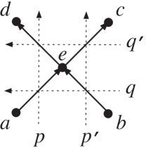
Figure 1: The square weight $U_{pp^{\prime}qq^{\prime}}(a,b,c,d)$ with sum over the central spin $e$. When $(x^{\vphantom{.}}_{q^{\prime}},y^{\vphantom{.}}_{q^{\prime}},\mu^{\vphantom{.}}_{q^{\prime}})=(y^{\vphantom{.}}_{q},\omega^{\ell}x^{\vphantom{.}}_{q},\mu_{q}^{-1})$, this can be arranged as a block-triangular array with $\ell\times\ell$ and $(N\!-\!\ell)\times(N\!-\!\ell)$ diagonal blocks $U_{pp^{\prime}q}^{(\ell)}(a,b,c,d)$ and $U_{pp^{\prime}q}^{(N-\ell)}(a,b,c,d)$ of $N\!\times\!N$ matrices. When also $(x^{\vphantom{.}}_{p^{\prime}},y^{\vphantom{.}}_{p^{\prime}},\mu^{\vphantom{.}}_{p^{\prime}})=(y^{\vphantom{.}}_{p},\omega^{j}x^{\vphantom{.}}_{p},\mu_{p}^{-1})$, these blocks further triangularize with diagonal blocks including the $j\times j$ block $U_{pq}^{(\ell,j)}(a,b,c,d)$. Setting $\ell=j=2$ this block gives six-vertex model weights at an $N$th root of unity. For general $\ell$ and $j$ the $U_{pq}^{(\ell,j)}(a,b,c,d)$ is a Boltzmann weight of a cyclic solid-on-solid (CSOS) model.

$$U_{pp^{\prime}qq^{\prime}}(a,b,c,d)=\sum_{e=1}^{N}W_{pq}(a-e){\overline{W}}_{pq^{\prime}}(e-d){\overline{W}}_{p^{\prime}q}(b-e)W_{p^{\prime}q^{\prime}}(e-c),$$ (1.3)

see figure 1, in which the four chiral Potts weights are given by

$$W_{pq}(n)=\Big{(}{\mu_{p}\over\mu_{q}}\Big{)}^{n}\prod_{m=1}^{n}\frac{y_{q}-x_{p}\omega^{m}}{y_{p}-x_{q}\omega^{m}},\quad\overline{W}_{pq}(n)=\big{(}{\mu_{p}\mu_{q}}\big{)}^{n}\prod_{m=1}^{n}\frac{\omega x_{p}-x_{q}\omega^{m}}{y_{q}-y_{p}\omega^{m}},$$ (1.4)

where the weights are periodic functions of $N$, $W(n+N)=W(n)$ and $\omega^{N}=1$. The subscripts $p$ and $q$ denote points on a high-genus curve, with each point $p$ parametrized by the triple $(x_{p},y_{p},\mu_{p})$ restricted by the conditions

$$k^{\prime}{}^{2}+k^{2}=1,\quad ky_{p}^{N}=1-k^{\prime}\mu_{p}^{N},\quad kx_{p}^{N}=1-k^{\prime}/\mu_{p}^{N},$$

$$t_{p}\equiv x_{p}y_{p},\quad k^{2}t_{p}^{N}=1+k^{\prime}{}^{2}-k^{\prime}(\lambda^{\vphantom{.}}_{p}+\lambda^{-1}_{p}),\quad\lambda^{\vphantom{.}}_{p}\equiv\mu^{N}_{p}.$$ (1.5)

In [14] they find that when $(x^{\vphantom{.}}_{q^{\prime}},y^{\vphantom{.}}_{q^{\prime}},\mu^{\vphantom{.}}_{q^{\prime}})=(y^{\vphantom{.}}_{q},\omega^{\ell}x^{\vphantom{.}}_{q},\mu_{q}^{-1})$, the square in (1.3) becomes block triangular: namely $U_{pp^{\prime}qq^{\prime}}(a,b,c,d)=0$ for $0\leq a-d\leq\ell-1$ and $\ell\leq b-c\leq N-1$. Now the diagonal blocks depend on the variable $t_{q}=x_{q}y_{q}$ only which no longer has to lie on a high-genus curve. Particularly, for $\ell=2$, the $2\times 2$ diagonal block $U_{pp^{\prime}q}^{(2)}(a,b,c,d)$ is related to $L$-operators like in (1.2).

If the vertical rapidities $p$ and $p^{\prime}$ are also related by $(x^{\vphantom{.}}_{p^{\prime}},y^{\vphantom{.}}_{p^{\prime}},\mu^{\vphantom{.}}_{p^{\prime}})=(y^{\vphantom{.}}_{p},\omega^{j}x^{\vphantom{.}}_{p},\mu_{p}^{-1})$, the diagonal block $U_{pp^{\prime}q}^{(2)}(a,b,c,d)$ is further decomposed, namely for $0\leq d-c\leq j-1$ and $j\leq a-b\leq N-1$, $U_{pp^{\prime}q}^{(2)}(a,b,c,d)=0$. Particularly for $j=2$, $U_{pp^{\prime}q}^{(2)}$ is block triangular, with one of its diagonal blocks related to a six-vertex model. The Yang–Baxter Equations of the chiral Potts model split into two sets of equations in IRF (Interaction-Round-a-Face) language as,

$$\sum^{N}_{g=1}{U}^{(2)}_{pp^{\prime}r}(a,g,e,f){U}_{pp^{\prime}q}^{(2)}(b,c,g,a){U}^{(2,2)}_{rq}(c,d,e,g)$$

$$=\sum^{N}_{g=1}{U}_{rq}^{(2,2)}(b,g,f,a){U}^{(2)}_{pp^{\prime}q}(g,d,e,f){U}^{(2)}_{pp^{\prime}r}(b,c,d,g).$$ (1.6)

shown in figure 2. We have, as in our previous papers [15, 16, 17], chosen the convention of multiplying from up to down, as seen from the above equation and in the figure 1.

Figure 2: Pictorial representation of Yang–Baxter equation (1.6).

The six-vertex $R$-matrix used by Bazhanov and Stroganov is different from the one descending from the chiral Potts model, creating subtle differences in the $\tau_{2}$-matrices in the two approaches. These differences are presented next.

1.3 Comparison of $R$-matrices of [13] and [14]

Bazhanov and Stroganov

$${\bf R}(x)=\left(\begin{array}[]{cccc}a&0&0&0\\ 0&b&xc&0\\ 0&c/x&{b}&0\\ 0&0&0&a\end{array}\right)\hfill$$ (1.11)

(1.12)

$$a=(x{\rm{q}}-x^{-1}{\rm{q}}^{-1}),\quad b=(x-x^{-1})$$ (1.13)

$$c=({\rm{q}}-{\rm{q}}^{-1}),\quad{\rm{q}}^{N}=1,\quad\hbox{$N$ odd}.$$ (1.14)

Descendant of Chiral Potts

$$U^{(2,2)}_{pq}=\left(\begin{array}[]{cccc}a&0&0&0\\ 0&b&tc&0\\ 0&c&{b/{\omega}}&0\\ 0&0&0&a\end{array}\right)\hfill$$ (1.19)

(1.20)

$$a=(1-\omega^{-1}t),\quad x^{2}=t=t_{q}/t_{p},\quad\omega^{N}=1,$$ (1.21)

$$b=(1-t),\quad c=(1-\omega^{-1}),\quad\hbox{any $N$}.$$ (1.22)

(1.23)

In the above comparison $\omega={\rm{q}}^{2}$. The transfer matrices for the symmetric six-vertex case on the left and the asymmetric one on the right are given respectively by

$$[T_{6v}]_{n,n^{\prime}}={\rm tr}\Bigg{[}\prod_{i=1}^{L}\sum_{m_{i}=0}^{1}{\bf R}_{n_{i},m_{i}}^{n^{\prime}_{i},m_{i+1}}(t)\Bigg{]},\quad[T_{a6v}]_{\sigma,\sigma^{\prime}}={\rm tr}\Bigg{[}\prod_{j=1}^{L}{\bf U}_{r,q}^{(2,2)}(\sigma^{\vphantom{.}}_{j},\sigma^{\vphantom{.}}_{j+1},\sigma^{\prime}_{j+1},\sigma^{\prime}_{j})\Bigg{]}.$$ (1.24)

Using Baxter’s well-known method—see e.g. chapter 10.14 of his book [18]—we can take the Hamiltonian limit and find

$$T_{6v} \to{\cal H}_{XXZ}=\sum_{j=1}^{L}\big{[}\sigma^{x}_{j}\sigma^{x}_{j+1}+\sigma^{y}_{j}\sigma^{y}_{j+1}+\Delta\sigma^{z}_{j}\sigma^{z}_{j+1}\big{]},\quad\Delta=\cos\frac{\pi}{N},$$ (1.25)

$$T_{a6v} \to{\cal H}_{XXX}+{\cal H}_{DM}=\sum_{j=1}^{L}\bigg{[}\Delta(\sigma^{x}_{j}\sigma^{x}_{j+1}+\sigma^{y}_{j}\sigma^{y}_{j+1}+\sigma^{z}_{j}\sigma^{z}_{j+1})$$ (1.26)

$$\hskip 101.17755pt+\sin\frac{\pi}{N}(\sigma^{x}_{j}\sigma^{y}_{j+1}-\sigma^{y}_{j}\sigma^{x}_{j+1})\bigg{]}.$$

This shows that, instead of the XXZ-spin chain Hamiltonian with periodic boundary conditions, the asymmetric case reduces to a periodic XXX chain with Dzyaloshinsky–Moriya term [19].

The $L$-operator of Bazhanov and Stroganov is

$${\cal L}_{j}(x)=\left[\begin{array}[]{cc}x^{-1}d_{-}{\bf X}^{-\rho}_{j}+xd_{+}{\bf X}^{\rho}_{j}&x(g_{+}{\bf X}^{-\rho}_{j}+g_{-}{\bf X}^{\rho}_{j}){\bf Z}^{\vphantom{.}}_{j}\\ x^{-1}(h_{+}{\bf X}^{-\rho}_{j}+h_{-}{\bf X}^{\rho}_{j}){\bf Z}_{j}^{-1}&x^{-1}f_{-}{\bf X}^{\rho}_{j}+xf_{+}{\bf X}^{-\rho}_{j}\end{array}\right],$$ (1.29)

(1.30)

$$h_{+}=d_{-}f_{+}/g_{+},\quad h_{-}=d_{+}f_{-}/g_{-},\quad\rho=(N-1)/2.$$ (1.31)

and the corresponding ${\boldsymbol{\tau}}^{\vphantom{{}^{\prime}}}_{2}(x)$ is given by

$${\boldsymbol{\tau}}^{\vphantom{{}^{\prime}}}_{2}(x)={\rm tr}[{\cal\bf L}(x)],\quad{\cal\bf L}(x)\equiv{\cal L}_{L}(x)\cdots{\cal L}_{j}(x)\cdots{\cal L}_{1}(x),\quad x^{2}=t_{q}.$$ (1.32)

However, ${\boldsymbol{\tau}}^{\vphantom{{}^{\prime}}}_{2}(t_{q})$ descending from the chiral Potts model is

$${\boldsymbol{\tau}}^{\vphantom{{}^{\prime}}}_{2}(t_{q})={\rm tr}[{\boldsymbol{\cal U}}(t_{q})],\quad{\boldsymbol{\cal U}}(t_{q})\equiv\prod_{i=1}^{L}{\bf U}_{p^{{}^{\vphantom{.}}}_{i}p^{\prime}_{i},q}^{(2)}(\sigma^{\vphantom{.}}_{i},\sigma^{\vphantom{.}}_{i+1},\sigma^{\prime}_{i+1},\sigma^{\prime}_{i}),$$ (1.33)

with $0\leq\sigma_{i}-\sigma^{\prime}_{i}\leq 1$ for $1\leq i\leq L+1$, without imposing the periodic boundary condition, where

$${\bf U}^{(2)}_{pp^{\prime}q}=\left[\begin{array}[]{cc}1-\omega{t_{q}}{\bf Z}/y_{p}y_{p^{\prime}}&{-\omega t_{q}}\mu_{p^{\prime}}(1-{x_{p^{\prime}}}{\bf Z}/{y_{p}}){\bf X}/{y_{p^{\prime}}}\\ {\mu_{p}}{\bf X}^{-1}(1-{\bf Z}{x_{p}}/{y_{p^{\prime}}})/{y_{p}}&{\mu_{p}\mu_{p^{\prime}}}(\omega x_{p}x_{p^{\prime}}{\bf Z}-\omega t_{q})/{y_{p}y_{p^{\prime}}}\end{array}\right].$$ (1.36)

In (1.31) and (1.36), we have

$${\bf Z}=\left(\begin{array}[]{ccccc}1&0&0&\cdots&0\\ 0&\omega&0&\cdots&0\\ 0&0&\omega^{2}&\cdots&0\\ \vdots&\ddots&\ddots&\ddots&\vdots\\ 0&\cdots&0&0&\omega^{N-1}\end{array}\right),\quad{\bf X}=\left(\begin{array}[]{ccccc}0&0&0&\cdots&1\\ 1&0&0&\cdots&0\\ 0&1&0&\cdots&0\\ \vdots&\ddots&\ddots&\ddots&\vdots\\ 0&\cdots&0&1&0\end{array}\right),$$ (1.37)

and

$${\bf X}_{j}=\hbox{\vbox{\hbox{${}_{1}$}\hbox{${\bf 1}$}}}\otimes\hbox{\vbox{\hbox{\;${}_{\cdots}$}\hbox{$\cdots$}}}\otimes{\bf 1}\otimes\hbox{\vbox{\hbox{\;${}_{j}$}\hbox{${\bf X}$}}}\otimes{\bf 1}\otimes\hbox{\vbox{\hbox{\;${}_{\cdots}$}\hbox{$\cdots$}}}\otimes\hbox{\vbox{\hbox{${}_{L}$}\hbox{${\bf 1}$}}}\,,$$

$${\bf Z}_{j}=\hbox{\vbox{\hbox{${}_{1}$}\hbox{${\bf 1}$}}}\otimes\hbox{\vbox{\hbox{\;${}_{\cdots}$}\hbox{$\cdots$}}}\otimes{\bf 1}\otimes\hbox{\vbox{\hbox{\;${}_{j}$}\hbox{${\bf Z}$}}}\otimes{\bf 1}\otimes\hbox{\vbox{\hbox{\;${}_{\cdots}$}\hbox{$\cdots$}}}\otimes\hbox{\vbox{\hbox{${}_{L}$}\hbox{${\bf 1}$}}}\,.$$ (1.38)

It is worthwhile to note that, even though we use the same ${\bf Z}$ and ${\bf X}$ in both cases, in (1.31) the matrices act on spin variables $\sigma_{i}$, but in (1.36) they act on edge variables $n_{i}=\sigma_{i}-\sigma_{i+1}$ mod $N$, such that ${\bf Z}_{j}|\{n_{i}\}\rangle=\omega^{n_{i}}|\{n_{i}\}\rangle$ and ${\bf X}_{j}|\{n_{i}\}\rangle=|n_{1},\cdots,n_{i}+1,\cdots,n_{L}\rangle$.

The monodromy matrix in (1.32),

$${\bf L}(x)=\left[\begin{array}[]{cc}{\bf A}(x)&{\bf B}(x)\cr{\bf C}(x)&{\bf D}(x)\end{array}\right]=\sum_{n=-L}^{L}\,x^{n}\left[\begin{array}[]{cc}{\bf A}_{n}&{\bf B}_{n}\cr{\bf C}_{n}&{\bf D}_{n}\end{array}\right],$$ (1.39)

satisfies the Yang–Baxter equation

$$[{\cal\bf L}(x)\otimes{\cal\bf L}(y)]{\bf{\check{R}}}(x/y)={\bf{\check{R}}}(x/y)[{\cal\bf L}(y)\otimes{\cal\bf L}(x)].$$ (1.40)

It is easy to show that ${\bf A}_{n}$ and ${\bf D}_{n}$ are nonvanishing only for even $n$, while ${\bf B}_{n}$ and ${\bf C}_{n}$ are nonzero for odd $n$. On the other hand, the monodromy matrix in (1.33) is

$${\boldsymbol{\cal U}}(t_{q})=\left[\begin{array}[]{cc}{\bf A}(t_{q})&{\bf B}(t_{q})\cr{\bf C}(t_{q})&{\bf D}(t_{q})\end{array}\right]=\sum_{n=0}^{L}\,(-\omega t_{q})^{n}\left[\begin{array}[]{cc}{\bf A}_{n}&{\bf B}_{n}\cr{\bf C}_{n}&{\bf D}_{n}\end{array}\right],$$ (1.41)

with nonnegative indices $n$ for the coefficients and ${\bf B}_{0}={\bf C}_{L}=0$. From repeated application of the Yang–Baxter equation (1.6) one can show that a similar Yang–Baxter equation holds for this monodromy matrix,

$$[{\boldsymbol{\cal U}}(t_{r})\otimes{\boldsymbol{\cal U}}(t_{q})]{\bf U}^{(2,2)}_{rq}={\bf U}^{(2,2)}_{rq}[{\boldsymbol{\cal U}}(t_{q})\otimes{\boldsymbol{\cal U}}(t_{r})].$$ (1.42)

Both Yang–Baxter equations (1.42) and (1.40) give rise to sixteen relations between the ${\bf A}(t)$, ${\bf B}(t)$, ${\bf C}(t)$ and ${\bf D}(t)$. By changing the vertical rapidity variables, or changing the size (or length) $L$, we change the monodromy matrices, but that does not change the Yang–Baxter equations. Thus, the sixteen relations remain the same in each of the two cases. However, the differences in the six-vertex $R$-matrices shown in (1.23) cause the sixteen relations to be different for the two cases (1.39) and (1.41).

1.4 Degenerate eigenspace in XXZ model and superintegrable $\tau_{2}$ model

For the superintegrable chiral Potts model, it was shown in [22, 23, 24, 25, 26] that there exist special sets of $2_{{}^{\vphantom{.}}}^{m_{E}}$ Ising-like eigenvalues of the transfer matrix or Hamiltonian, which implies a $2_{{}^{\vphantom{.}}}^{m_{E}}$-fold degeneracy in the corresponding $\tau_{2}$ model. Superintegrability means that the model satisfies two or more different integrability criteria, like Yang–Baxter or Onsager algebra integrability [2, 23]. In their study of the XXZ model at roots of unity [27, 28, 29, 30], the authors show the existence of a quantum loop algebra $L({\widehat{\mathfrak{sl}}}_{2})$ in the XXZ model. Such a loop algebra or subalgebra was also shown in [15, 16, 17, 31, 32] to exist in certain sectors of the superintegrable ${\boldsymbol{\tau}}^{\vphantom{{}^{\prime}}}_{2}$-model. The proof of this degeneracy is based on the sixteen relations of the Yang–Baxter equations. Since the equations (1.6) are model-independent, one needs to know why there is degeneracy in the superintegrable ${\boldsymbol{\tau}}^{\vphantom{{}^{\prime}}}_{2}$ model, but not in the generic ${\boldsymbol{\tau}}^{\vphantom{{}^{\prime}}}_{2}$ model.

1.5 Understanding the degeneracy

Consider two of the sixteen equations obtained from (1.42),

$$(\omega y-x){\bf A}(x){\bf B}(y)=\omega(y-x){\bf B}(y){\bf A}(x)+y(\omega-1){\bf A}(y){\bf B}(x),$$ (1.43)

$$(\omega y-x){\bf B}(y){\bf D}(x)=(y-x){\bf D}(x){\bf B}(y)+y(\omega-1){\bf B}(x){\bf D}(y).$$ (1.44)

Equating the coefficients of $x^{L+1}$ of these two equations, we find

$${\bf A}_{L}{\bf B}(y)=\omega{\bf B}(y){\bf A}_{L},\quad{\bf B}(y){\bf D}_{L}={\bf D}_{L}{\bf B}(y).$$ (1.45)

Similarly by equating the coefficients of $y^{L+1}$, we have

$${\bf A}(x){\bf B}_{L}-{\bf B}_{L}{\bf A}(x)=(1-\omega^{-1}){\bf A}_{L}{\bf B}(x)=-(1-\omega){\bf B}(x){\bf A}_{L},$$

$${\bf D}(x){\bf B}_{L}-\omega{\bf B}_{L}{\bf D}(x)=(1-\omega){\bf D}_{L}{\bf B}(x)=(1-\omega){\bf B}(x){\bf D}_{L}.$$ (1.46)

By induction, one can show

$${\bf A}(x){\bf B}^{n}_{L}-{\bf B}^{n}_{L}{\bf A}(x)=-(1-\omega)[n]{\bf B}(x){\bf B}^{n-1}_{L}{\bf A}_{L},$$

$${\bf D}(x){\bf B}^{n}_{L}-\omega^{n}{\bf B}^{n}_{L}{\bf D}(x)=(1-\omega)[n]{\bf B}(x){\bf B}^{n-1}_{L}{\bf D}_{L}.$$ (1.47)

so that

$$[{\bf A}(x)+{\bf D}(x)]{\bf B}^{(n)}_{L}-{\bf B}^{(n)}_{L}[{\bf A}(x)+\omega^{n}{\bf D}(x)]=(\omega-1){\bf B}(x){\bf B}^{(n-1)}_{L}[{\bf A}_{L}-{\bf D}_{L}].$$ (1.48)

Here we have used the definitions

$${\bf B}^{(n)}_{L}=\frac{{\bf B}^{\,n}_{L}}{[n]!},\qquad[n]=\frac{1-\omega^{n}}{1-\omega},\quad[n]!=\prod_{k=1}^{n}\,[k].$$ (1.49)

Letting $n=N$ in (1.48), and using $\omega^{N}=1$, we find both ${\bf B}^{\,N}_{L}=0$ and $[N]!=0$. However, ${\bf B}^{(N)}_{L}$ can be defined through a limiting procedure [32], so that

$$[{\boldsymbol{\tau}}^{\vphantom{{}^{\prime}}}_{2}(x),{\bf B}^{(N)}_{L}]=[{\bf A}(x)+{\bf D}(x),{\bf B}^{(N)}_{L}]=(\omega-1){\bf B}(x){\bf B}^{(N-1)}_{L}[{\bf A}_{L}-{\bf D}_{L}].$$ (1.50)

This shows that the degeneracy of the eigenspace of an eigenvalue depends on the difference ${\bf A}_{L}-{\bf D}_{L}$. For, if $|\Psi\rangle$ is an eigenvector of ${\boldsymbol{\tau}}^{\vphantom{{}^{\prime}}}_{2}(x)$ and $[{\bf A}_{L}-{\bf D}_{L}]|\Psi\rangle=0$, then $[{\boldsymbol{\tau}}^{\vphantom{{}^{\prime}}}_{2}(x),{\bf B}^{(N)}_{L}]|\Psi\rangle=0$. Consequently, ${\bf B}^{(N)}_{L}|\Psi\rangle$ is also an eigenvector with same eigenvalue.

For the generic case, we can show that ${\bf B}^{N}_{L}\neq 0$, but constant, so that ${\bf B}^{N}_{L}|\Psi\rangle$ does not give rise to an independent eigenvector, and its eigenspace is nondegenerate.

From (1.36) we have

$${\bf A}_{0}=1, {\bf D}_{0}=\omega^{L}\prod_{j=1}^{L}\frac{{\bf Z}_{j}\mu_{p^{\vphantom{.}}_{j}}\mu_{p^{\prime}_{j}}x_{p^{\vphantom{.}}_{j}}x_{p^{\prime}_{j}}}{y_{p^{\vphantom{.}}_{j}}y_{p^{\prime}_{j}}},$$

$${\bf A}_{L}=\prod_{j=1}^{L}\frac{{\bf Z}_{j}}{y_{p^{\vphantom{.}}_{j}}y_{p^{\prime}_{j}}},\quad {\bf D}_{L}=\prod_{j=1}^{L}\frac{\mu_{p^{\vphantom{.}}_{j}}\mu_{p^{\prime}_{j}}}{y_{p^{\vphantom{.}}_{j}}y_{p^{\prime}_{j}}}.\quad$$ (1.51)

Consider the lattice with periodic boundary condition $\sigma_{L+1}=\sigma_{1}$, so that

$$\sum_{i=1}^{L}n_{i}=\sum_{i=1}^{L}(\sigma_{i}-\sigma_{i+1})=\sigma_{1}-\sigma_{L+1}=0.$$ (1.52)

Then we have $\prod_{j=1}^{L}{\bf Z}_{j}|\{n_{i}\}\rangle=|\{n_{i}\}\rangle$. Consequently, if $\mu_{p_{j}}\mu_{p^{\prime}_{j}}=1$, for all $j$, then ${\boldsymbol{\tau}}^{\vphantom{{}^{\prime}}}_{2}$ has degenerate eigenspaces. From (1.5), we find the condition $\mu_{p}\mu_{p^{\prime}}=1$ is satisfied if and only if $(x_{p^{\prime}},y_{p^{\prime}},\mu_{p^{\prime}})=(y^{\vphantom{.}}_{p},\omega^{j}x^{\vphantom{.}}_{p},\mu_{p}^{-1})$. This is indeed the case for the superintegrable case with $j=N$.

1.6 CSOS models

In the context of the eight-vertex model Baxter [33, 34] has introduced the restricted solid-on-solid (rSOS) model , in which an interface is described by assigning integer heights to the sites of a two-dimensional lattice, while restricting the heights (or height differences) to a finite range. Pearce and Seaton [35] chose a different restriction, choosing the heights from some $\mathbb{Z}_{N}$ using the cyclic condition $N+1\equiv 1$, calling their model a cyclic solid-on-solid (CSOS) model. Here we shall introduce other examples of CSOS models.

As mentioned above, it has been shown in [14] that for $(x_{q^{\prime}},y_{q^{\prime}},\mu_{q^{\prime}})=(y^{\vphantom{.}}_{q},\omega^{\ell}x^{\vphantom{.}}_{q},\mu_{q}^{-1})$ and $(x_{p^{\prime}},y_{p^{\prime}},\mu_{p^{\prime}})=(y^{\vphantom{.}}_{p},\omega^{j}x^{\vphantom{.}}_{p},\mu_{p}^{-1})$, the square $U_{pp^{\prime}qq^{\prime}}(a,b,c,d)=0$ for $0\leq a-d\leq\ell-1$ and $\ell\leq b-c\leq N-1$; and also for $0\leq d-c\leq j-1$ and $j\leq a-b\leq N-1$. The diagonal block $U^{(\ell,j)}_{pq}(a,b,c,d)$ describes a special case of the CSOS model with $0\leq a-d,b-c\leq\ell-1$ and $0\leq d-c,a-b\leq j-1$, and depends on $t_{q}$ and $t_{p}$ only. Its weights, which are left implicit in [14] are given in (2.106) in the Appendix. The corresponding transfer matrices, denoted by ${\boldsymbol{\tau}}^{\vphantom{{}^{\prime}}}_{\ell,j}$, are special cases of the ${\boldsymbol{\tau}}^{\vphantom{{}^{\prime}}}_{\ell}$ model acting on restricted spaces with $0\leq n_{i}\leq j-1$.

1.7 Outline of the paper

In section 2, we consider the special case of such a CSOS model with $\ell=2$, so that its monodromy matrix satisfies the Yang–Baxter equation (1.42). The eigenvectors of this model are given in section 2.2. In section 3, we use the method of Baxter [26] to derive the Drinfeld polynomial of the highest-weight representation which shows that the CSOS model has $2^{m_{E}}$-fold degeneracy for some integers $m_{E}$, which will be given later. This in turn means the existence of quantum loop algebras. The generators of the quantum loop algebra given in (4.17) are the same as those given in [17]. In section 4, we shall present the proof of the Serre relations for these generators for the CSOS models, which includes the superintegrable case.

Included in the Appendix A is rederivation of the decomposition of the square of weights, as the notations used in [14] are not conventional. The corresponding functional relations for the product of two transfer matrices given in [14, 26] for these CSOS models are included here in Appendix B. As the functional relations between the ${\boldsymbol{\tau}}^{\vphantom{{}^{\prime}}}_{j}$-matrices are direct consequences of fusion, it is shown in Appendix B.2, that the T-system functional relations studied by many authors [37, 38, 39] also hold for any ${\boldsymbol{\tau}}^{\vphantom{{}^{\prime}}}_{j}$ model. In Appendix C, the relationships between the coefficients of the monodromy matrix (1.41), which only depend on the specific form of the asymmetric 6-vertex model $R$-matrix, are given. Using these relations, we also show in section 4, that ${\bf C}_{L-1}$, ${\bf B}_{L}$, ${\bf C}_{0}$ and ${\bf B}_{1}$ of the CSOS models are related to a $j^{L}$-dimensional representation of $U_{\rm q}(\widehat{\mathfrak{sl}}_{2})$.

2 CSOS models for $\ell=2$

Using alternating horizontal and vertical rapidities,

$$(x_{q^{\prime}},y_{q^{\prime}},\mu_{q^{\prime}})=(y^{\vphantom{.}}_{q},\omega^{2}x^{\vphantom{.}}_{q},\mu_{q}^{-1})\quad\hbox{and}\quad(x_{p^{\prime}},y_{p^{\prime}},\mu_{p^{\prime}})=(y^{\vphantom{.}}_{p},\omega^{j}x^{\vphantom{.}}_{p},\mu_{p}^{-1}),$$ (2.1)

we have the decomposition of the square

$$U_{pp^{\prime}qq^{\prime}}(a,b,c,d)\to U^{(2)}_{pp^{\prime}q}(a,b,c,d){(t_{q})}\to U^{(2,j)}_{pq}(a,b,c,d){(t_{q}/t_{p})},$$ (2.2)

and from (1.36), we find the nonvanishing elements to be

$${\bf U}^{(2,j)}_{pq}(a,b,b,a)=1-\omega^{1-j+a-b}t, \quad 0\leq a-b\leq j-1;$$

$${\bf U}^{(2,j)}_{pq}(a,b,b-1,a)=-\omega^{1-j}t(1-\omega^{1+a-b}), \quad 0\leq a-b\leq j-2;$$

$${\bf U}^{(2,j)}_{pq}(a,b,b,a-1)=1-\omega^{a-b-j}, \quad 1\leq a-b\leq j-1;$$

$${\bf U}^{(2,j)}_{pq}(a,b,b-1,a-1)=\omega^{1-j}(\omega^{a-b}-t), \quad 0\leq a-b\leq j-1.$$ (2.3)

where we set $t=t_{q}/t_{p}$, so that the high-genus rapidities are replaced by the usual rapidities with difference property. The resulting transfer matrix is

$$[{\boldsymbol{\tau}}^{\vphantom{{}^{\prime}}}_{2,j}(t_{q}/t_{p})]_{\sigma,\sigma^{\prime}}={\rm tr}[{\boldsymbol{\cal U}}^{(2,j)}(t)],\quad{\boldsymbol{\cal U}}^{(2,j)}(t)\equiv\prod_{j=1}^{L}{\bf U}_{p,q}^{(2,j)}(\sigma^{\vphantom{.}}_{j},\sigma^{\vphantom{.}}_{j+1},\sigma^{\prime}_{j+1},\sigma^{\prime}_{j}).$$ (2.4)

Since $\ell=2$, the Yang–Baxter equations (1.6) or (1.42) hold for the monodromy matrix ${\boldsymbol{\cal U}}^{(2,j)}(t)$. As can be seen from (2.3), the weights are simpler than those studied by Pearce and Seaton and others [35, 40].

2.1 Commutation relation for $\ell=2$.

For $0\leq d-c,a-b\leq j-1$, using (2.3), we find the leading coefficients to be

$${\bf A}_{0}=1,\quad{\bf D}_{0}=\omega^{(1-j)L}\prod_{i=1}^{L}{\bf Z}^{(j)}_{i},\quad{\bf A}_{L}=\omega^{-jL}\prod_{i=1}^{L}{\bf Z}_{i}^{(j)},\quad{\bf D}_{L}=\omega^{-jL},$$ (2.5)

where ${\bf Z}^{(j)}$ is the $j\times j$ diagonal matrix with elements

$${\bf Z}^{(j)}_{k,l}=\delta_{k,l}\omega^{k},\quad 0\leq k,l\leq j-1.$$ (2.6)

From (2.3), we find that the weights depend only on the difference of neighboring spins. As the transfer matrices of the CSOS models commute with the spin shift operator $\mbox{\mycal X}={\bf X}_{1}{\bf X}_{2}\cdots{\bf X}_{L}$, their eigenspaces split into $N$ blocks. In the block corresponding to the eigenvalue $\omega^{Q}$ of the shift operator X, the transfer matrix becomes ${\bf A}(t)+\omega^{-Q}{\bf D}(t)$. Assuming cyclic boundary conditions and $L$ a multiple of $N$, $L=pN$ for some integer $p$, we find from (2.5) that the same commutation relations

$$[{\bf A}(x)+\omega^{-Q}{\bf D}(x),{\bf C}_{0}^{(nN+Q)}{\bf B}_{1}^{(mN+Q)}]\,|\{n_{j}\}\rangle=0,$$

$$[{\bf A}(x)+\;\omega^{Q}\,{\bf D}(x),{\bf B}_{1}^{(mN+Q)}{\bf C}_{0}^{(nN+Q)}]\,|\{n_{j}\}\rangle=0,$$

$$[{\bf A}(x)+\omega^{-Q}{\bf D}(x),{\bf B}_{L}^{(mN+Q)}{\bf C}_{L-1}^{(nN+Q)}]\,|\{n_{j}\}\rangle=0,$$

$$[{\bf A}(x)+\;\omega^{Q}\,{\bf D}(x),{\bf C}_{L-1}^{(nN+Q)}{\bf B}_{L}^{(mN+Q)}]\,|\{n_{j}\}\rangle=0,$$ (2.7)

hold as those given in (IV:49) and (IV:50) of [17].

Thus the generators of $L({\widehat{\mathfrak{sl}}}_{2})$ for the ground-state sectors in superintegrable models, as given in [31, 32, 15] for $Q=0$ and in [17] for $Q\neq 0$, should also be generators for the CSOS model. To show that CSOS models with weights given by (2.3) support quantum loop algebra $L({\widehat{\mathfrak{sl}}}_{2})$ in all sectors, we must prove that the generators satisfy the necessary Serre relations; this proof will be given in section 4. We shall first present vectors, upon which these generators generate eigenspaces spanned by $2^{m_{E}}$ eigenvectors having the same eigenvalue.

2.2 Eigenvectors

It is easily verified that Yang–Baxter equation (1.42) also holds for the monodromy matrix ${\boldsymbol{\cal U}}(t_{q})$ with different vertical rapidities, as defined in (1.33). Therefore, the well-known identities derived in [21, 32] also hold for this monodromy matrix, i.e.

$${\bf A}(x_{0})\Bigg{(}\prod_{i=1}^{R}{\bf B}(x_{i})\Bigg{)}=\omega^{R}\Bigg{[}\Bigg{(}\prod_{i=1}^{R}f_{i0}\Bigg{)}\Bigg{(}\prod_{i=1}^{R}{\bf B}(x_{i})\Bigg{)}{\bf A}(x_{0})$$ (2.8)

$$\hskip 80.0pt+\sum_{i=1}^{R}\Bigg{(}\prod_{k=1,k\neq i}^{R}f_{ki}\Bigg{)}g_{0i}\Bigg{(}\prod_{k=0,k\neq i}^{R}{\bf B}(x_{k})\Bigg{)}{\bf A}(x_{i})\Bigg{]},$$ (2.9)

$${\bf D}(x_{0})\Bigg{(}\prod_{i=1}^{R}{\bf B}(x_{i})\Bigg{)}=\omega^{R}\Bigg{[}\Bigg{(}\prod_{i=1}^{R}f_{0i}\Bigg{)}\Bigg{(}\prod_{i=1}^{R}{\bf B}(x_{i})\Bigg{)}{\bf D}(x_{0})$$ (2.10)

$$\hskip 80.0pt-\sum_{i=1}^{R}\Bigg{(}\prod_{k=1,k\neq i}^{R}f_{ik}\Bigg{)}g_{0i}\Bigg{(}\prod_{k=0,k\neq i}^{R}{\bf B}(x_{k})\Bigg{)}{\bf D}(x_{i})\Bigg{]},$$ (2.11)

where we used the short-hand notations of [32],

$$f_{ik}=f\bigg{(}\frac{x_{i}}{x_{k}}\bigg{)},\quad g_{ik}=g\bigg{(}\frac{x_{i}}{x_{k}}\bigg{)},\quad f(z)=\frac{z-\omega}{\omega(z-1)},\quad g(z)=\frac{1-\omega}{\omega(z-1)}.$$ (2.12)

Similarly, we also have

$${\bf A}(x_{0})\Bigg{(}\prod_{i=1}^{R}{\bf C}(x_{i})\Bigg{)}=\Bigg{[}\Bigg{(}\prod_{i=1}^{R}f_{0i}\Bigg{)}\Bigg{(}\prod_{i=1}^{R}{\bf C}(x_{i})\Bigg{)}{\bf A}(x_{0})$$ (2.13)

$$\hskip 80.0pt+\sum_{i=1}^{R}\Bigg{(}\prod_{k=1,k\neq i}^{R}f_{ik}\Bigg{)}g_{i0}\Bigg{(}\prod_{k=0,k\neq i}^{R}{\bf C}(x_{k})\Bigg{)}{\bf A}(x_{i})\Bigg{]},$$ (2.14)

$${\bf D}(x_{0})\Bigg{(}\prod_{i=1}^{R}{\bf C}(x_{i})\Bigg{)}=\Bigg{[}\Bigg{(}\prod_{i=1}^{R}f_{i0}\Bigg{)}\Bigg{(}\prod_{i=1}^{R}{\bf C}(x_{i})\Bigg{)}{\bf D}(x_{0})$$ (2.15)

$$\hskip 80.0pt-\sum_{i=1}^{R}\Bigg{(}\prod_{k=1,k\neq i}^{R}f_{ki}\Bigg{)}g_{i0}\Bigg{(}\prod_{k=0,k\neq i}^{R}{\bf C}(x_{k})\Bigg{)}{\bf D}(x_{i})\Bigg{]}.$$ (2.16)

In these equations, the subscripts are different from those of Nishino and Deguchi [32], because of the difference in the $R$-matrices.

Consider the vector $|{\bf R}\rangle$ given by

$$|{\bf R}\rangle={\bf B}^{(\ell N-R)}_{L}\prod_{i=1}^{R}{\bf B}(x_{i})|\Omega\rangle,\quad|\Omega\rangle=|\{0\}\rangle=\binrel@{\binrel@{\mbox{\Large$\otimes$}}\binrel@@{\mathop{\kern 0.0pt\mbox{\Large$\otimes$}}\limits_{j=1}}}\binrel@@{\mathop{\kern 0.0pt\binrel@{\mbox{\Large$\otimes$}}\binrel@@{\mathop{\kern 0.0pt\mbox{\Large$\otimes$}}\limits_{j=1}}}\limits^{L}}|0\rangle.$$ (2.17)

Here $|\Omega\rangle$ is the state $|\{n_{i}\}\rangle$ with all $n_{i}=\sigma_{i}-\sigma_{i+1}$ having the minimal value 0. Then, using the commutation relations (1.47), we find

$$[{\bf A}(t)+\omega^{-Q}{\bf D}(t)|{\bf R}\rangle={\bf B}^{(\ell N-R)}_{L}[{\bf A}(t)+\omega^{-Q-R}{\bf D}(t)]\prod_{i=1}^{R}{\bf B}(x_{i})|\Omega\rangle$$

$$+{(\omega-1){\bf B}^{(\ell N-R-1)}_{L}{\bf B}(t)\prod_{i=1}^{R}{\bf B}(x_{i})(\omega^{R}{\bf A}_{L}-\omega^{-Q}{\bf D}_{L})|\Omega\rangle}.$$ (2.18)

Note that the second term in (2.18) vanishes if either $R=\ell N$ or $R=nN-Q$. If $R=\ell N$, the first line reproduces (2.18); if $R=nN-Q$, we can use (2.5) and $\prod_{i=1}^{L}{\bf Z}_{i}^{(j)}|\Omega\rangle=|\Omega\rangle$, which follows from (2.6). Also we find from (2.3) that

$${\bf A}(t)|\Omega\rangle=a(t)|\Omega\rangle,\quad a(t)=(1-\omega^{1-j}t)^{L},$$

$${\bf D}(t)|\Omega\rangle=d(t)|\Omega\rangle,\quad d(t)=\omega^{(1-j)L}(1-t)^{L}.$$ (2.19)

Next set $x_{0}=t$ and define

$$F(t)=\prod_{i=1}^{R}(t-\omega x_{i}),$$ (2.20)

so that, with $f_{ij}$ defined by (2.12),

$$\prod_{i=1}^{R}f_{0i}=\frac{F(t)}{F(\omega t)},\quad\prod_{i=1}^{R}f_{i0}=\omega^{-R}\frac{F(\omega^{2}t)}{F(\omega t)},\quad\prod_{k=1,k\neq i}^{R}\frac{f_{ik}}{f_{ki}}=\prod_{k=1,k\neq i}^{R}\frac{x_{i}-\omega x_{k}}{\omega x_{i}-x_{k}}.$$ (2.21)

Then, using the identities (2.11) and (2.19) in (2.18), we obtain

$$[{\bf A}(t)+\omega^{-Q}{\bf D}(t)]|{\bf R}\rangle=\bigg{[}a(t)\frac{F(\omega^{2}t)}{F(\omega t)}+\omega^{-Q}d(t)\frac{F(t)}{F(\omega t)}\bigg{]}|{\bf{R}}\rangle$$

$$+{\bf B}^{(\ell N-R)}_{L}\sum_{i=1}^{R}g_{0i}\prod_{k=0,k\neq i}^{R}{\bf B}(x_{k})\prod_{k=1,k\neq i}^{R}[\omega(x_{i}-x_{k})]^{-1}$$

$$\times{\bigg{[}a(x_{i})\omega^{R}\prod_{k=1,k\neq i}^{R}(\omega x_{i}-x_{k})-d(x_{i})\omega^{-Q}\prod_{k=1,k\neq i}^{R}(x_{i}-\omega x_{k})\bigg{]}}|\Omega\rangle,$$ (2.22)

where we have also used (2.21) and (2.12). If we choose the $x_{i}$ for $i=1,\cdots,R$ such that

$$a(x_{i})\omega^{R}\prod_{k=1,k\neq i}^{R}(\omega x_{i}-x_{k})=d(x_{i})\omega^{-Q}\prod_{k=1,k\neq i}^{R}(x_{i}-\omega x_{k}),$$ (2.23)

which are actually the Bethe Ansatz equations, then the second term in (2.22) vanishes. Then $|{\bf R}\rangle$ is an eigenvector of $[{\bf A}(t)+\omega^{-Q}{\bf D}(t)]$ with eigenvalue

$$T_{\mathrm{CSOS}}=\tau_{2,j}(t) =\bigg{[}a(t)\frac{F(\omega^{2}t)}{F(\omega t)}+\omega^{-Q}d(t)\frac{F(t)}{F(\omega t)}\bigg{]}$$ (2.24)

$$=\bigg{[}(1-\omega^{1-j}t)^{L}\frac{F(\omega^{2}t)}{F(\omega t)}+\omega^{-Q+(1-j)L}(1-t)^{L}\frac{F(t)}{F(\omega t)}\bigg{]}.$$

Similarly, let

$$|{\bar{\Omega}}\rangle=|\{j-1\}\rangle=\binrel@{\binrel@{\mbox{\Large$\otimes$}}\binrel@@{\mathop{\kern 0.0pt\mbox{\Large$\otimes$}}\limits_{j=1}}}\binrel@@{\mathop{\kern 0.0pt\binrel@{\mbox{\Large$\otimes$}}\binrel@@{\mathop{\kern 0.0pt\mbox{\Large$\otimes$}}\limits_{j=1}}}\limits^{L}}|j-1\rangle$$ (2.25)

be the state $|\{n_{i}\}\rangle$ with all $n_{i}=\sigma_{i}-\sigma_{i+1}$ having the maximal value $j-1$. It is easy to see from (2.3) that

$${\bf A}(t)|{\bar{\Omega}}\rangle={\hat{a}}(t)|{\bar{\Omega}}\rangle,\quad{\hat{a}}(t)=(1-t)^{L},$$

$${\bf D}(t)|{\bar{\Omega}}\rangle={\hat{d}}(t)|{\bar{\Omega}}\rangle,\quad{\hat{d}}(t)=(1-\omega^{1-j}t)^{L}.$$ (2.26)

Consider now the vector

$$|{\bf{\bar{R}}}\rangle={\bf C}^{(\ell N-R)}_{L-1}\prod_{i=1}^{R}{\bf C}(x_{i})|{\bar{\Omega}}\rangle.$$ (2.27)

Using the commutation relations

$${\bf C}(x){\bf A}_{L}=\omega{\bf A}_{L}{\bf C}(x),\qquad{\bf C}(x){\bf D}_{L}={\bf D}_{L}{\bf C}(x),$$

$${\bf A}(x){\bf C}^{(n)}_{L-1}={\bf C}^{(n)}_{L-1}{\bf A}(x)+(\omega-1)\omega^{1-n}x{\bf C}^{{(n-1)}}_{L-1}{\bf C}(x){\bf A}_{L},$$

$${\bf D}(x){\bf C}^{(n)}_{L-1}=\omega^{-n}{\bf C}^{(n)}_{L-1}{\bf D}(x)-(\omega-1)\omega^{1-n}x{\bf C}^{(n-1)}_{L-1}{\bf C}(x){\bf D}_{L},$$ (2.28)

we can easily show that, if $R=\ell N$ or $R=nN+Q$ and $\{x_{1},x_{2},\cdots,x_{R}\}$ satisfy the Bethe Ansatz equations

$${\hat{a}}(x_{i})\prod_{k=1,k\neq i}^{R}(x_{i}-\omega x_{k})=\omega^{R-Q}{\hat{d}}(x_{i})\prod_{k=1,k\neq i}^{R}(\omega x_{i}-x_{k}),$$ (2.29)

then $|{\bf\bar{R}}\rangle$ is also an eigenvector of $[{\bf A}(t)+\omega^{-Q}{\bf D}(t)]$ and has eigenvalue

$${T}_{\mathrm{CSOS}}=\tau_{2,j}(t)= \bigg{[}{\hat{a}}(t)\frac{F(t)}{F(\omega t)}+\omega^{-Q}{\hat{d}}(t)\frac{F(\omega^{2}t)}{F(\omega t)}\bigg{]}$$ (2.30)

$$=\bigg{[}(1-t)^{L}\frac{F(t)}{F(\omega t)}+\omega^{(1-j)L-Q}(1-\omega^{1-j}t)^{L}\frac{F(\omega^{2}t)}{F(\omega t)}\bigg{]},$$

where we have added $\omega^{(1-j)L}=1$ in the second line to make the result also valid if $L\neq pN$. However, for $L\neq pN$, $|{\bar{\Omega}}\rangle$ does not satisfy the cyclic boundary condition, so that the vectors (2.27) are not eigenvectors under that condition.

However, the vectors given by

$$|\hat{\bf R}\rangle={\bf B}^{(\ell N-R)}_{1}\prod_{i=1}^{R}{\bf B}(x_{i})|\Omega\rangle,\quad\omega^{R}=\omega^{Q-(1-j)L},\quad R\neq\ell N,$$ (2.31)

with the $x_{i}$ for $i=1,\cdots,R$ satisfying the Bethe Ansatz equations

$$(1-x_{i})^{L}\prod_{k=1,k\neq i}^{R}(x_{i}-\omega x_{k})=(1-\omega^{1-j}x_{i})^{L}\prod_{k=1,k\neq i}^{R}(\omega x_{i}-x_{k}),$$ (2.32)

can be shown to be eigenvectors with eigenvalues given by (2.30).

From finite-size calculations, we find that these are not the only possibilities. We must also introduce

$$|\tilde{\bf R}\rangle={\bf B}^{(\ell N-R-n)}_{L}{\bf B}^{(n)}_{1}\prod_{i=1}^{R}{\bf B}(x_{i})|\Omega\rangle,\quad\omega^{R}=\omega^{-Q-n}=\omega^{(j-1)L},$$ (2.33)

with the $x_{i}$ satisfying the Bethe Ansatz equations

$$\omega^{Q}(1-x_{i})^{L}\prod_{k=1,k\neq i}^{R}(x_{i}-\omega x_{k})=(1-\omega^{1-j}x_{i})^{L}\prod_{k=1,k\neq i}^{R}(\omega x_{i}-x_{k}).$$ (2.34)

Their eigenvalues are also given by (2.30).

We can summarize the results rewriting (2.24) and (2.30) as

$$\tau_{2,j}(t)F(\omega t)=\omega^{-P_{a}}(1-t)^{L}{F(t)}+\omega^{P_{b}}(1-\omega^{1-j}t)^{L}{F(\omega^{2}t)},$$ (2.35)

where we must choose $-P_{a}=(1-j)L-Q\;{\rm{mod}}\;N$ and $P_{b}=0$ in (2.24) and $P_{a}=0$ and $P_{b}=(1-j)L-Q\;{\rm{mod}}\;N$ in (2.30). Then the Bethe Ansatz equations become

$$(1-x_{i})^{L}\prod_{k=1,k\neq i}^{R}(x_{i}-\omega x_{k})=\omega^{P_{a}+P_{b}+R}(1-\omega^{1-j}x_{i})^{L}\prod_{k=1,k\neq i}^{R}(\omega x_{i}-x_{k}).$$ (2.36)

These results include the superintegrable case when $j=N$.

The eigenvalues (2.35) are easily seen to be independent of the $\ell$ in (2.17), (2.27), (2.31), and (2.33), which also shows the degeneracy of their eigenspaces. The smallest allowed values of $\ell$ lead to the possible highest-weight vectors.

Thus, we have shown that the eigenvectors are degenerate, but we have not yet demonstrated the Ising-like behavior with $2^{m_{E}}$-fold degeneracies. To understand the degeneracy, we must calculate the highest-weight polynomials, or the so-called Drinfeld polynomials [28, 29, 32]. We shall use the method of Baxter in [26] to determine these polynomials. As a byproduct, the eigenvalues of all our CSOS models for any $\ell$ are explicitly given.

3 Functional relations in CSOS models

3.1 Explicit formula for $\tau_{\ell,j}(t)$

Using $-P_{a}+P_{b}=(1-j)L-Q$, we rewrite the functional relation (2.109) as

$$\tau_{2,j}(\omega^{\ell-1}t)\tau_{\ell,j}(t)-\omega^{-P_{a}+P_{b}}(1-\omega^{\ell-1}t)^{L}(1-\omega^{\ell-1-j}t)^{L}\tau_{\ell-1,j}(t)=\tau_{\ell+1,j}(t).$$ (3.1)

We shall show by induction that

$$\tau_{\ell,j}(t)=\sum_{n=0}^{\ell-1}\zeta_{n}^{\ell,j}(t),\qquad 2\leq\ell\leq N,$$ (3.2)

$$\zeta_{n}^{\ell,j}(t)\equiv\frac{\omega^{nP_{b}-(\ell-1-n)P_{a}}F(t)F(\omega^{\ell}t)}{F(\omega^{\ell-n-1}t)F(\omega^{\ell-n}t)}\prod_{m=0}^{\ell-2-n}(1-\omega^{m}t)^{L}\prod_{m=\ell-n}^{\ell-1}(1-\omega^{m-j}t)^{L},$$ (3.3)

for the eigenvalues $\tau_{\ell,j}(t)$ of ${\boldsymbol{\tau}}^{\vphantom{{}^{\prime}}}_{\ell,j}(t)$. It is easy to see that for $\ell=2$, we have

$$\zeta_{0}^{2,j}(t)=\frac{\omega^{-P_{a}}F(t)}{F(\omega t)}(1-t)^{L},\quad\zeta_{1}^{2,j}(t)=\frac{\omega^{P_{b}}F(\omega^{2}t)}{F(\omega t)}(1-\omega^{1-j}t)^{L},$$ (3.4)

so that $\tau_{2,j}$ is identical to (2.35). Now assume (3.2) holds for $\ell$ or smaller. Using (3.2) and (3.3), we can easily show

$$\zeta_{0}^{2,j}(\omega^{\ell-1}t)\zeta_{0}^{\ell,j}(t)=\omega^{-\ell P_{a}}\frac{F(t)}{F(\omega^{\ell}t)}\prod_{m=0}^{\ell-1}(1-\omega^{m}t)^{L},$$ (3.5)

$$\zeta_{0}^{2,j}(\omega^{\ell-1}t)\,\big{[}\tau_{\ell,j}(t)-\zeta_{0}^{\ell,j}(t)\big{]}=\zeta_{0}^{2,j}(\omega^{\ell-1}t)\sum_{n=0}^{\ell-2}\zeta_{n+1}^{\ell,j}(t)$$

$$=\omega^{-P_{a}+P_{b}}(1-\omega^{\ell-1}t)^{L}(1-\omega^{\ell-1-j}t)^{L}\tau_{\ell-1,j}(t),$$ (3.6)

$$\zeta_{1}^{2,j}(\omega^{\ell-1}t)\tau_{\ell,j}(t)=\sum_{n=0}^{\ell-1}\frac{\omega^{(n+1)P_{b}-(\ell-n-1)P_{a}}F(t)F(\omega^{\ell+1}t)}{F(\omega^{\ell-n-1}t)F(\omega^{\ell-n}t)}$$

$$\times\prod_{m=0}^{\ell-2-n}(1-\omega^{m}t)^{L}\prod_{m=\ell-n}^{\ell}(1-\omega^{m-j}t)^{L}.$$ (3.7)

Also, $\tau_{2,j}(\omega^{\ell-1}t)\tau_{\ell,j}(t)$ in (3.1) is the sum of the left-hand sides of (3.5), (3.6) and (3.7), while the right-hand side of (3.6) cancels the second term of (3.1). Therefore, replacing $n=n^{\prime}-1$ in (3.7),we obtain the desired result

$$\tau_{\ell+1,j}(t)=\sum_{n=0}^{\ell}\frac{\omega^{nP_{b}-(\ell-n)P_{a}}F(t)F(\omega^{\ell+1}t)}{F(\omega^{\ell-n}t)F(\omega^{\ell-n+1}t)}\prod_{m=0}^{\ell-1-n}(1-\omega^{m}t)^{L}\prod_{m=\ell+1-n}^{\ell}(1-\omega^{m-j}t)^{L}.$$ (3.8)

This proves (3.2) holds for all $\ell\leq N$.

3.2 Functional relations for the transfer matrices

Following the method of Baxter in chapter 6 of [26], we introduce

$$T_{q}=N^{{\scriptstyle{\frac{1}{2}}}L}\frac{(1-x_{q}/y_{p})^{L}}{(1-x^{N}_{q}/y^{N}_{p})^{L}}{\cal T}(x_{q},y_{q}),\quad{\hat{T}}_{q^{\prime}}=N^{{\scriptstyle{\frac{1}{2}}}L}\frac{(1-\omega^{-j}y_{q}/x_{p})^{L}}{(1-y_{q}^{N}/x_{p}^{N})^{L}}{\hat{\cal T}}(y_{q},\omega^{\ell}x_{q}).$$ (3.9)

It has been shown by Baxter [26] or can be seen from (2.103) that ${\cal T}(x_{q},y_{q})$ and ${\hat{\cal T}}(y_{q}\omega^{\ell},x_{q})$ are polynomials in $x_{q}$ and $y_{q}$. Let $t=t_{q}/t_{p}$, so that (2.104) for $\ell=1,\cdots,N$ becomes

$${\cal T}(x_{q},y_{q}){\hat{\cal T}}(y_{q},\omega^{\ell}x_{q})=\Bigg{(}\prod_{m=\ell}^{N-1}(1-\omega^{m-j}t)^{L}\Bigg{)}{\boldsymbol{\tau}}^{\vphantom{{}^{\prime}}}_{\ell,j}(t)$$

$$+\omega^{\ell(P_{b}-P_{a})}\Bigg{(}\prod_{m=0}^{\ell-1}(1-\omega^{m}t)^{L}\Bigg{)}{\boldsymbol{\tau}}^{\vphantom{{}^{\prime}}}_{N-\ell,j}(\omega^{\ell}t).$$ (3.10)

Now substituting (3.2) into (3.10), we find that its eigenvalues become

$${\cal T}(x_{q},y_{q}){\hat{\cal T}}(y_{q},\,\omega^{\ell}x_{q})=\omega^{\ell P_{b}}\Bigg{(}\prod_{m=0}^{N-1-j}(1-\omega^{m}t)^{L}\Bigg{)}F(t)F(\omega^{\ell}t)\,t^{P_{a}+P_{b}}\,{\cal P}(t^{N}),$$ (3.11)

where

$$t_{q}^{P_{a}+P_{b}}{\cal P}(t^{N})=\omega^{-P_{b}}\sum_{k=0}^{N-1}\frac{\omega^{-k(P_{a}+P_{b})}}{F(\omega^{k}t)F(\omega^{k+1}t)}\prod_{n=1}^{j-1}(1-\omega^{k-n}t)^{L}.$$ (3.12)

For $j=N$, this reduces to the result for the superintegrable case examined by Baxter in [26]. It is also easily seen that the degree of ${\cal P}(t^{N})$ is $m_{E}=\lfloor\big{(}L(j-1)-2R-P_{a}-P_{b}\big{)}/N\rfloor$. From (1.5) we find that we may write

$${\cal P}(t_{q}^{N}/t_{p})=G(\lambda_{q})G(\lambda^{-1}_{q}),\qquad\lambda_{q}=\mu_{q}^{N}.$$ (3.13)

3.3 Analysis of the transfer matrices and their eigenvalues

Using (Baxter:2.22), we find

$$T(\omega x_{q},\omega^{-1}y_{q})=\left[\frac{(y_{p}-\omega x_{q})(y_{q}-\omega^{1+j}x_{p})}{(y_{q}-\omega x_{p})\omega(y_{p}-x_{q})}\right]^{L}{\mbox{\mycal X}}^{-1}T(x_{q},y_{q}),$$

$${\hat{T}}(\omega y_{q},\omega^{-1}x_{q})=\left[\frac{(x_{q}-\omega y_{p})(\omega^{j}x_{p}-\omega y_{q})}{(x_{p}-y_{q})\omega(x_{q}-\omega y_{p})}\right]^{L}{\mbox{\mycal X}}^{-1}{\hat{T}}(y_{q},x_{q}).$$ (3.14)

Similarly, we can show

$$T(\omega^{-1}x_{q},\omega y_{q})=\left[\frac{(y_{q}-x_{p})(\omega y_{p}-x_{q})}{(y_{p}-x_{q})(y_{q}-\omega^{j}x_{p})}\right]^{L}{\mbox{\mycal X}}\,T(x_{q},y_{q}),$$

$${\hat{T}}(\omega^{-1}y_{q},\omega x_{q})=\left[\frac{(\omega x_{p}-y_{q})(x_{q}-y_{p})}{(x_{q}-y_{p})(\omega^{j}x_{p}-y_{q})}\right]^{L}{\mbox{\mycal X}}\,{\hat{T}}(y_{q},x_{q}).$$ (3.15)

Therefore, when the shift operator X is replaced by $\omega^{-Q}$, the rescaled polynomial transfer matrices defined in (3.9) restricted to the sector corresponding to $Q$, satisfy

$${\cal T}(\omega x_{q},\omega^{-1}y_{q})=\omega^{P_{a}-P_{b}} \left[\frac{1-\omega^{-1-j}y_{q}/x_{p}}{1-\omega^{-1}y_{q}/x_{p}}\right]^{L} {\cal T}(x_{q},y_{q}),$$ (3.16)

$${\hat{\cal T}}(\omega y_{q},\omega^{-1}x_{q})=\omega^{P_{a}-P_{b}} \left[\frac{1-\omega^{-j}y_{q}/x_{p}}{1-y_{q}/x_{p}}\right]^{L} {\hat{\cal T}}(y_{q},x_{q}),$$ (3.17)

$${\cal T}(\omega^{-1}x_{q},\omega y_{q})=\omega^{-P_{a}+P_{b}} \left[\frac{1-y_{q}/x_{p}}{1-\omega^{-j}y_{q}/x_{p}}\right]^{L} {\cal T}(x_{q},y_{q}),$$ (3.18)

$${\hat{\cal T}}(\omega^{-1}y_{q},\omega x_{q})=\omega^{-P_{a}+P_{b}} \left[\frac{1-\omega^{-1}y_{q}/x_{p}}{1-\omega^{-1-j}y_{q}/x_{p}}\right]^{L} {\hat{\cal T}}(y_{q},x_{q}),$$ (3.19)

where $P_{a}-P_{b}=(j-1)L+Q$, since we have chosen the multiplication from up-to-down. If one prefers Baxter’s convention, one needs to make the change of $Q\to-Q$. When $j=N$, this reduces to the superintegrable case in (Baxter:6.5) with $r=0$ as it should.

For $(x_{p^{\prime}},y_{p^{\prime}},\mu_{p^{\prime}})=(y_{p},\omega^{j}x_{p},\mu_{p}^{-1})$, we can use (BBP:2.20) and (BBP:2.44) to show

$$\frac{f_{p^{\prime}q}f_{pr}}{f_{pq}f_{p^{\prime}r}}=\frac{(1-x_{q}/y_{p})(1-\omega^{-j}x_{r}/x_{p})(1-x^{N}_{q}/x^{N}_{p})(1-x^{N}_{r}/y^{N}_{p})}{(1-x^{N}_{q}/y^{N}_{p})(1-x^{N}_{r}/x^{N}_{p})(1-\omega^{-j}x_{q}/x_{p})(1-x_{r}/y_{p})}$$

$$\times\prod_{n=N-j}^{N-1}\frac{(1-\omega^{n}t_{r}/t_{p})(1-\omega^{n}x_{q}/x_{p})(1-\omega^{n}y_{q}/x_{p})}{(1-\omega^{n}t_{q}/t_{p})(1-\omega^{n}x_{r}/x_{p})(1-\omega^{n}y_{r}/x_{p})},$$ (3.20)

with $f_{pq}$ defined in [3, equation (13)]. The commutation relation (Baxter:2.12) can then be rewritten for the rescaled transfer matrices in (3.9) as

$${\cal T}(x_{q},y_{q}){\hat{\cal T}(x_{r},y_{r})}={\cal T}(x_{r},y_{r}){\hat{\cal T}(x_{q},y_{q})}$$

$$\times\prod_{n=N-j}^{N-1}\Bigg{[}\frac{(1-\omega^{n}t_{r}/t_{p})(1-\omega^{n}x_{q}/x_{p})(1-\omega^{n}y_{q}/x_{p})}{(1-\omega^{n}t_{q}/t_{p})(1-\omega^{n}x_{r}/x_{p})(1-\omega^{n}y_{r}/x_{p})}\Bigg{]}^{L}.$$ (3.21)

This relation holds for any $q$ and $r$, which suggest that

$${\hat{\cal T}(x_{q},y_{q})}=\kappa\,{\cal T}(x_{q},y_{q})\prod_{n=N-j}^{N-1}\Bigg{[}\frac{(1-\omega^{n}t_{q}/t_{p})}{(1-\omega^{n}x_{q}/x_{p})(1-\omega^{n}y_{q}/x_{p})}\Bigg{]}^{L}.$$ (3.22)

where $\kappa$ is some constant. Now we can use (3.16) to (3.19) and (3.22) to find the transfer matrix eigenvalues, such that (3.11) is satisfied. Let us write

$${\cal T}(x_{q},y_{q})=x_{q}^{P_{a}}y_{q}^{P_{b}}\lambda_{q}^{-P_{c}}G(\lambda_{q}^{-1})F(t_{q})\prod_{n=0}^{N-j-1}\frac{(1-\omega^{n}t_{q}/t_{p})^{L}}{(1-\omega^{n}y_{q}/x_{p})^{L}},$$ (3.23)

where $P_{a}$, $P_{b}$ and $P_{c}$ are integers in the interval $0\leq P_{a},P_{b},P_{c}\leq N-1$. We suggest that (3.23) is still a polynomial as the zeroes in the denominators are cancelled out by the zeroes in the numerator. If $x_{p}=\omega^{n}y_{q}$, then $\lambda^{-1}_{p}=\lambda_{q}$, so that $\lambda_{p}=\lambda^{-1}_{q}$ or $y_{p}^{N}=x_{q}^{N}$. Thus we find $t_{p}^{N}=t_{q}^{N}$. There is an $N$-sheet branch cut structure for variables $x_{q},y_{q}$ and $t_{q}$, but we may choose the sheet so that $t_{p}=\omega^{n}t_{q}$. Thus ${\cal T}(x_{q},y_{q})$ is free of poles. The expression (3.23) for ${\cal T}(x_{q},y_{q})$ can be easily shown to satisfy (3.16) and (3.18). From (3.23), we have

$${\cal T}(y_{q},x_{q})=y_{q}^{P_{a}}x_{q}^{P_{b}}\lambda_{q}^{P_{c}}G(\lambda_{q})F(t_{q})\prod_{n=0}^{N-j-1}\frac{(1-\omega^{n}t_{q}/t_{p})^{L}}{(1-\omega^{n}x_{q}/x_{p})^{L}}.$$ (3.24)

Now we use (3.22) to obtain

$${\hat{\cal T}(y_{q},x_{q})}=\kappa y_{q}^{P_{a}}x_{q}^{P_{b}}\lambda_{q}^{P_{c}}G(\lambda_{q})F(t_{q})\prod_{n=0}^{N-1}\frac{(1-\omega^{n}t_{q}/t_{p})^{L}}{(1-\omega^{n}x_{q}/x_{p})^{L}}\prod_{n=N-j}^{N-1}\frac{1}{(1-\omega^{n}y_{q}/x_{p})^{L}}.$$ (3.25)

Using (1.5), we may write

$$\prod_{n=0}^{N-1}\frac{1-\omega^{n}t_{q}/t_{p}}{1-\omega^{n}x_{q}/x_{p}}=\frac{1-t^{N}_{q}/t^{N}_{p}}{1-x^{N}_{q}/x^{N}_{p}}=-\frac{\mu^{N}_{p}x^{N}_{p}}{k^{\prime}y_{p}^{N}}\bigg{(}1-\frac{y^{N}_{q}}{x^{N}_{p}}\bigg{)}=\kappa^{-1/L}\prod_{n=0}^{N-1}\bigg{(}1-\frac{\omega^{n}y_{q}}{x_{p}}\bigg{)}$$ (3.26)

with $\kappa^{1/L}=-k^{\prime}y_{p}^{N}/\mu^{N}_{p}x^{N}_{p}$, so that (3.25) becomes

$${\hat{\cal T}(y_{q},x_{q})}=y_{q}^{P_{a}}x_{q}^{P_{b}}\lambda_{q}^{P_{c}}G(\lambda_{q})F(t_{q})\prod_{n=0}^{N-1-j}{(1-\omega^{n}y_{q}/x_{p})^{L}}.$$ (3.27)

It can again easily verified that ${\hat{\cal T}(y_{q},x_{q})}$ as given by (3.27) satisfies the relations (3.17) and (3.19). Furthermore, substituting (3.23) and (3.27) into (3.11), we find it becomes an identity. As explained in [26], we find from (1.5) that, in the limit $\mu_{q}\to 0$, $x_{q}\to\infty$, while $y_{q}$, $x_{q}\mu_{q}$ remain finite. This means that the weights in (1.4) are finite, and so are $T_{q}$ and ${\hat{T}}_{q^{\prime}}$. From (3.9), we find then that ${\cal T}(x_{q},y_{q})$ diverges no faster than $x_{q}^{(N-1)L}$ and ${\hat{\cal T}}(y_{q},x_{q})$ stays finite. In this limit, we find from (3.27) and (3.23) that

$${\hat{\cal T}}(y_{q},x_{q})\to x_{q}^{P_{b}-NP_{c}+R},\quad{\cal T}(x_{q},y_{q})\to x_{q}^{P_{a}+NP_{c}+Nm_{E}+R+(N-j)L}.$$ (3.28)

Thus if we choose the integer $P_{c}$ such that

$$P_{b}+R\leq NP_{c}\leq(j-1)L-m_{E}N-P_{a}-R,$$ (3.29)

then ${\hat{\cal T}}(y_{q},x_{q})$ is finite, and ${\cal T}(x_{q},y_{q})$ is $\mathrm{O}(x_{q}^{(N-1)L})$. Similarly, in the limit $\mu_{q}\to\infty$, we find from (1.5) that $y_{q}\to\infty$, while $x_{q}$, $y_{q}/\mu_{q}$ remain finite, such that

$${\cal T}(x_{q},y_{q})\to y_{q}^{P_{b}-NP_{c}+R},\quad{\hat{\cal T}}(y_{q},x_{q})\to y_{q}^{P_{a}+NP_{c}+Nm_{E}+R+(N-j)L}.$$ (3.30)

The condition in (3.29) then guarantees that ${\cal T}(x_{q},y_{q})$ is finite and ${\hat{\cal T}}(y_{q},x_{q})$ diverges no faster than $y_{q}^{L(N-1)}$, as it should.

4 Serre relations of the quantum loop algebra $L({\mathfrak{sl}}_{2})$ for the generators

The superintegrable chiral Potts models are found to have Ising-like spectra [22, 23, 25], and here we have shown that our CSOS models behave similarly.

For $Q=0$ and $L$ a multiple of $N$, it has been shown [31, 32] that the eigenspace in the superintegrable case supports a quantum loop algebra $L({\mathfrak{sl}}_{2})$. Furthermore, this loop algebra can be decomposed into $r=\lfloor(N-1)L/N\rfloor$ simple ${\mathfrak{sl}}_{2}$ algebras [15, 16, 17].

For the $Q\neq 0$ cases, we have assumed in [17] that the Serre relations hold. Even though, we have shown these relation to hold when operated on some special vectors, see Appendix B of [17], and also tested them extensively by computer for small systems, a proof was still lacking. In this section, we shall present the proof for the CSOS model, which includes the superintegrable case as a special case.

We shall first show that ${\bf C}_{L-1}$, ${\bf B}_{L}$, ${\bf C}_{0}$ and ${\bf B}_{1}$ for the CSOS models are related to a $j^{L}$-dimensional representation of the affine quantum group $U_{\rm q}(\widehat{\mathfrak{sl}}_{2})$. Therefore, the higher-order quantum Serre relation in Proposition 7.1.5 of Lusztig [41] holds also for the CSOS model. From (2.3) and (1.41), we find

$${\bf B}_{L}=\omega^{-jL}\sum_{n=1}^{L}\Bigg{(}\prod_{m=1}^{n-1}{\bf Z}^{(j)}_{m}\Bigg{)}\,\hat{\mbox{\bfrak f}}_{n},\quad{\bf C}_{0}=\sum_{n=1}^{L}\omega^{(n-1)(1-j)}\Bigg{(}\prod_{m=1}^{n-1}{\bf Z}^{(j)}_{m}\Bigg{)}\,\hat{\mbox{\bfrak e}}_{n},$$

$${\bf B}_{1}=\omega^{-j}\sum_{n=1}^{L}\,\omega^{(L-n)(1-j)}\hat{\mbox{\bfrak f}}_{n}\prod_{m=n+1}^{L}{\bf Z}^{(j)}_{m},\quad{\bf C}_{L-1}=\omega^{-j(L-1)}\sum_{n=1}^{L}\,\hat{\mbox{\bfrak e}}_{n}\prod_{m=n+1}^{L}{\bf Z}^{(j)}_{m},$$ (4.1)

where ${\bf Z}^{(j)}$ is the $j\times j$ diagonal matrix obtained by deleting the last $N-j$ columns and rows of ${\bf Z}$. Let ${\bf X}^{(j)}$ denote the $j\times j$ singular matrix obtained by deleting the last $N-j$ columns and rows of ${\bf X}$, The other operators in (4.1) are

$$\hat{\mbox{\bfrak e}}_{n}=({\bf X}_{n}^{(j)})^{T}(1-\omega^{-j}{\bf Z}^{(j)}_{n}),\quad\hat{\mbox{\bfrak f}}_{n}=(1-{\bf Z}^{(j)}_{n}){\bf X}^{(j)}_{n}.$$ (4.2)

4.1 Representations of $U_{\rm q}({\mathfrak{sl}}_{2})$

The equations in Appendix C are valid for any $L$. If we let $L=1$, the three equations in (3.136) and (3.137) become one,

$${\bf C}_{0}{\bf B}_{1}-\omega{\bf B}_{1}{\bf C}_{0}=(1-\omega)[{\bf D}_{1}{\bf A}_{0}-{\bf D}_{0}{\bf A}_{1}].$$ (4.3)

From (4.1), we find ${\bf B}_{1}=\omega^{-j}\hat{\mbox{\bfrak f}}_{1}$, and ${\bf C}_{0}=\hat{\mbox{\bfrak e}}_{1}$. From (2.5), we get ${\bf D}_{1}{\bf A}_{0}=\omega^{-j}$ and ${\bf D}_{0}{\bf A}_{1}=\omega^{1-2j}({\bf Z}_{1}^{(j)})^{2}$. Next we let ${\rm q}^{2}=\omega$, ${\bf Z}_{1}^{(j)}={\bf Q}_{1}^{\;2}$ and

$${\bf T}^{-2}=\omega^{1-j}({\bf Z}_{1}^{(j)})^{2},\quad{\bf B}_{1}=({\rm q}-{\rm q}^{-1})\mu{\bf T}^{-{\scriptstyle{\frac{1}{2}}}}{\bf F},\quad{\bf C}_{0}=({\rm q}-{\rm q}^{-1})\nu{\bf E}{\bf T}^{-{\scriptstyle{\frac{1}{2}}}},$$ (4.4)

where $\mu=-\omega^{-j}{\rm{q}}^{{\scriptstyle{\frac{1}{2}}}(j-1)}$ and $\nu={\rm{q}}^{{\scriptstyle{\frac{1}{2}}}(-j-1)}$. Then we have

$${\bf T}^{-1}{\bf F}={\rm q}^{2}{\bf F}{\bf T}^{-1},\quad{\bf T}{\bf E}={\rm q}^{2}{\bf E}{\bf T}.$$ (4.5)

Substituting (4.4) into (4.3), and using (4.5), we find

$$({\bf E}{\bf F}-{\bf F}{\bf E})=({\bf T}-{\bf T}^{-1})\big{/}({\rm q}-{\rm q}^{-1}).$$ (4.6)

Thus ${\bf T}$, ${\bf E}$ and ${\bf F}$ are generators of $U_{\rm q}({\mathfrak{sl}}_{2})$.

4.2 Representations of $U_{\rm q}({\widehat{\mathfrak{sl}}}_{2})$

For $L\geq 2$, we find from (2.5) that

$${\bf D}_{L}{\bf A}_{0}=\omega^{-jL},\quad{\bf D}_{0}{\bf A}_{L}=\omega^{(1-2j)L}\prod_{i=1}^{L}({\bf Z}_{i}^{(j)})^{2}=\omega^{-jL}{\bf T}_{0}^{-2},$$ (4.7)

defining generator ${\bf T}_{0}$. We obtain further generators from

$${\bf B}_{L}=({\rm q}-{\rm q}^{-1})\mu^{\vphantom{.}}_{0}{\bf T}_{0}^{-{\scriptstyle{\frac{1}{2}}}}{\bf F}^{\vphantom{.}}_{0},\quad{\bf C}_{0}=({\rm q}-{\rm q}^{-1})\nu^{\vphantom{.}}_{0}{\bf E}^{\vphantom{.}}_{0}{\bf T}_{0}^{-{\scriptstyle{\frac{1}{2}}}},\quad{\bf T}^{\vphantom{.}}_{1}={\bf T}^{-1}_{0},$$

$${\bf B}_{1}=({\rm q}-{\rm q}^{-1})\mu^{\vphantom{.}}_{1}{\bf T}_{0}^{-{\scriptstyle{\frac{1}{2}}}}{\bf E}^{\vphantom{.}}_{1},\quad{\bf C}_{L-1}=({\rm q}-{\rm q}^{-1})\nu^{\vphantom{.}}_{1}{\bf F}^{\vphantom{.}}_{1}{\bf T}_{0}^{-{\scriptstyle{\frac{1}{2}}}},$$ (4.8)

where

$$\mu_{0}=-\omega^{-jL}{\rm{q}}^{-{\scriptstyle{\frac{1}{2}}}(j-1)},\quad \nu_{0}={\rm{q}}^{{\scriptstyle{\frac{1}{2}}}(j-1)-1},$$

$$\mu_{1}=-\omega^{-j}{\rm{q}}^{{\scriptstyle{\frac{1}{2}}}(j-1)-L(j-1)},\quad \nu_{1}=\omega^{-j(L-1)}{\rm{q}}^{-{\scriptstyle{\frac{1}{2}}}(j+1)+L(j-1)}.$$ (4.9)

It is easily shown that with $\alpha_{ii}=2$ and $\alpha_{ij}=-2$, we have for $0\leq i,j\leq 1$ the relations

$${\bf T}_{i}^{-1}{\bf F}^{\vphantom{.}}_{j}={\rm q}^{\alpha_{ij}}{\bf F}^{\vphantom{.}}_{j}{\bf T}_{i}^{-1},\quad{\bf T}^{\vphantom{.}}_{i}{\bf E}^{\vphantom{.}}_{j}={\rm q}^{\alpha_{ij}}{\bf E}^{\vphantom{.}}_{j}{\bf T}^{\vphantom{.}}_{i},$$ (4.10)

Substituting (4.8) into (3.136), and using (4.9) and (4.10), we find

$${\bf E}_{i}{\bf F}_{j}-{\bf F}_{j}{\bf E}_{i}=\delta_{i,j}({\bf T}^{\vphantom{.}}_{i}-{\bf T}_{i}^{-1})\big{/}({\rm q}-{\rm q}^{-1}).$$ (4.11)

We also need the following definitions for the scaled powers,

$${\bf B}_{\ell}^{(n)}=\frac{{\bf B}_{\ell}^{\,n}}{[n]!},\quad{\bf C}_{\ell}^{(n)}=\frac{{\bf C}_{\ell}^{\,n}}{[n]!},\quad[n]!=\prod_{\ell=1}^{n}\frac{1-\omega^{\ell}}{1-\omega},$$

$${\bf E}_{i}^{(n)}=\frac{{\bf E}_{i}^{\,n}}{[n]_{\rm{q}}!},\quad{\bf F}_{i}^{(n)}=\frac{{\bf F}_{i}^{\,n}}{[n]_{\rm{q}}!},\quad[n]_{\rm{q}}!=\prod_{\ell=1}^{n}\frac{{\rm{q}}^{\ell}-{\rm{q}}^{-\ell}}{{\rm{q}}-{\rm{q}}^{-1}},\quad[n]!={\rm q}^{{\scriptstyle{\frac{1}{2}}}n(n-1)}[n]_{\rm q}!,$$ (4.12)

from which we find

$${\bf C}^{\vphantom{.}}_{0}{\bf B}_{1}^{(3)}\propto{\rm q}^{6}{\bf E}^{\vphantom{.}}_{0}{\bf E}^{(3)}_{1}{\bf T}_{0}^{-2},\quad {\bf B}^{\vphantom{.}}_{1}{\bf C}^{\vphantom{.}}_{0}{\bf B}^{(2)}_{1}\propto{\rm q}^{6}{\bf E}^{\vphantom{.}}_{1}{\bf E}^{\vphantom{.}}_{0}{\bf E}^{(2)}_{1}{\bf T}_{0}^{-2},$$

$${\bf B}^{(2)}_{1}{\bf C}^{\vphantom{.}}_{0}{\bf B}^{\vphantom{.}}_{1}\propto{\rm q}^{4}{\bf E}^{\vphantom{.}}_{0}{\bf E}^{(3)}_{1}{\bf T}_{0}^{-2},\quad {\bf B}^{(3)}_{1}{\bf C}^{\vphantom{.}}_{0}\propto{\bf E}^{(3)}_{1}{\bf E}^{\vphantom{.}}_{0}{\bf T}_{0}^{-2}.$$ (4.13)

Similar relations hold for other combinations. Consequently, after canceling out the $\omega$-factors in (3.139) and (3.144), these relations become

$${\bf E}^{\vphantom{.}}_{i}{\bf E}^{(3)}_{j}-{\bf E}^{\vphantom{.}}_{j}{\bf E}^{\vphantom{.}}_{i}{\bf E}^{(2)}_{j}+{\bf E}^{(2)}_{j}{\bf E}^{\vphantom{.}}_{i}{\bf E}^{\vphantom{.}}_{j}-{\bf E}^{(3)}_{j}{\bf E}^{\vphantom{.}}_{i}=0,$$

$${\bf F}^{\vphantom{.}}_{i}{\bf F}^{(3)}_{j}-{\bf F}^{\vphantom{.}}_{j}{\bf F}^{\vphantom{.}}_{i}{\bf F}^{(2)}_{j}+{\bf F}^{(2)}_{j}{\bf F}^{\vphantom{.}}_{i}{\bf F}^{\vphantom{.}}_{j}-{\bf F}^{(3)}_{j}{\bf F}^{\vphantom{.}}_{i}=0,$$ (4.14)

for $i\neq j$ and $i,j=0,1$. This also shows that the $j^{L}\times j^{L}$ matrices ${\bf C}_{0}$, ${\bf B}_{1}$, ${\bf C}_{L-1}$ and ${\bf B}_{L}$ are related to the highest-weight representations of the affine quantum group $U_{\rm q}({\widehat{\mathfrak{sl}}}_{2})$, leaving out the discussion of the coproduct and other operators here. Consequently the higher-order quantum Serre relations in 7.1.6 of Lusztig [41] hold. If we define

$$({\rm{q}}-{\rm{q}}^{-1}){\mbox{\bfrak e'}}=({\bf X}^{(j)})^{T}{({\rm{q}}^{j}{\bf Q}^{-1}-{\rm{q}}^{-j}{\bf Q})},$$

$$({\rm{q}}-{\rm{q}}^{-1}){\mbox{\bfrak f'}}={({\bf Q}-{\bf Q}^{-1})}{\bf X}^{(j)},\qquad{\mbox{\bfrak t'}}={\rm{q}}^{j-1}{\bf Q}^{-2},$$ (4.15)

then the generators in (4.8) are explicitly given as

$${\bf E}_{0}=\sum_{n=0}^{L}{\rm{q}}^{-n(j-1)}\prod_{m=1}^{n-1}{\mbox{\bfrak t'}}_{m}^{-{\scriptstyle{\frac{1}{2}}}}{\mbox{\bfrak e'}}_{n}\prod_{m=n+1}^{L}{\mbox{\bfrak t'}}_{m}^{{\scriptstyle{\frac{1}{2}}}},\quad{\bf F}_{0}=\sum_{n=0}^{L}{\rm{q}}^{n(j-1)}\prod_{m=1}^{n-1}{\mbox{\bfrak t'}}_{m}^{-{\scriptstyle{\frac{1}{2}}}}{\mbox{\bfrak f'}}_{n}\prod_{m=n+1}^{L}{\mbox{\bfrak t'}}_{m}^{{\scriptstyle{\frac{1}{2}}}},$$

$${\bf F}_{1}=\sum_{n=0}^{L}{\rm{q}}^{-n(j-1)}\prod_{m=1}^{n-1}{\mbox{\bfrak t'}}_{m}^{{\scriptstyle{\frac{1}{2}}}}{\mbox{\bfrak e'}}_{n}\prod_{m=n+1}^{L}{\mbox{\bfrak t'}}_{m}^{-{\scriptstyle{\frac{1}{2}}}},\quad{\bf E}_{1}=\sum_{n=0}^{L}{\rm{q}}^{n(j-1)}\prod_{m=1}^{n-1}{\mbox{\bfrak t'}}_{m}^{{\scriptstyle{\frac{1}{2}}}}{\mbox{\bfrak f'}}_{n}\prod_{m=n+1}^{L}{\mbox{\bfrak t'}}_{m}^{-{\scriptstyle{\frac{1}{2}}}}.$$ (4.16)

4.3 Serre relation for the generators of the loop algebra

As in [17], the generators of the loop algebra are given by

$${\bf x}_{0,Q}^{+}\propto{\bf C}_{0}^{(N+Q)}{\bf B}_{1}^{(Q)},\quad{\bf x}_{1,Q}^{-}\propto{\bf C}_{0}^{(Q)}{\bf B}_{1}^{(N+Q)},$$

$${\bf x}_{-1,Q}^{+}\propto{\bf C}_{L-1}^{(N+Q)}{\bf B}_{L}^{(Q)},\quad{\bf x}_{0,Q}^{-}\propto{\bf C}_{L-1}^{(Q)}{\bf B}_{L}^{(N+Q)}.$$ (4.17)

For $Q=0$, each term in the Serre relation is a product of 4 operators. For $Q\neq 0$, each term in the Serre relation is a product of 8 operators. To prove the $Q\neq 0$ case, we need to move factors around. We shall first prove the identities

$${\bf C}_{0}^{(N+Q)}{\bf B}_{1}^{(Q)}{\bf C}_{0}^{(Q)}={\bf C}_{0}^{(Q)}{\bf B}_{1}^{(Q)}{\bf C}_{0}^{(N+Q)}.$$ (4.18)

As in Chapter 7 of Lusztig [41], but now for the cyclic case with ${\rm{q}}^{2N}=1$, we define

$$f_{i,j,n,m;e}=f_{n,m;e}=\sum_{r+s=m}(-1)^{r}{\rm{q}}^{er(2n-m+1)}\theta_{i}^{(r)}\theta_{j}^{(n)}\theta_{i}^{(s)},\quad i,j=0,1,\quad j\neq i,$$ (4.19)

where we may choose $e=\pm 1$, $\theta_{i}={\bf E}_{i}$ or $\theta_{i}={\bf F}_{i}$, and $\theta_{i}^{(r)}=\theta_{i}^{r}/[r]_{\rm{q}}!$. It is shown by Lusztig in Proposition 7.15.(b) [41] that if $m>2n$, then $f_{n,m;e}=0$. For $n=1$, and $m=3$, this is the usual quantum Serre relation given in (4.14). We follow the steps of Lusztig in his proof. Since $f_{n,m-\ell;e}=0$ for $\ell\leq m-2n-1$, we have

$$g=\sum_{\ell=0}^{m-2n-1}(-1)^{\ell}{\rm{q}}^{\ell(1-m)}f^{\vphantom{.}}_{n,m-\ell;1}\theta_{i}^{(\ell)}=0.$$ (4.20)

Using (4.19), we find

$$g =\sum_{\ell=0}^{m-2n-1}\sum_{r+s^{\prime}=m-\ell}(-1)^{\ell+r}{\rm{q}}^{\ell(1-m)+r(2n-m+\ell+1)}\theta_{i}^{(r)}\theta_{j}^{(n)}\theta_{i}^{(s^{\prime})}\theta_{i}^{(\ell)}$$ (4.21)

$$=\sum_{s=0}^{m}c_{s}\,\theta_{i}^{(m-s)}\theta_{j}^{(n)}\theta_{i}^{(s)}=0,\quad s=s^{\prime}+\ell,\quad r=m-s,$$

where

$$\qquad c_{s}=\sum_{\ell=0}^{m-2n-1}(-1)^{\ell+m-s}{\rm{q}}^{\ell(1-s)+(m-s)(2n-m+1)}\Bigg{[}\begin{array}[]{@{}c@{}}s\\ \ell\end{array}\Bigg{]}_{\rm{q}},\quad\Bigg{[}\begin{array}[]{@{}c@{}}s\\ \ell\end{array}\Bigg{]}_{\rm{q}}=\frac{[s]_{\rm{q}}!}{[\ell]_{\rm{q}}![s-\ell]_{\rm{q}}!}.$$ (4.22)

These are exactly the same as in [41]. But from now on, we will use the cyclic property as in [27]. We let $s=kN+p$ for $0\leq k\leq\lfloor m/N\rfloor$, and $0\leq p\leq p_{k}$, where for $0\leq k\leq\lfloor m/N\rfloor-1$, $p_{k}=N-1$, but $p_{\lfloor m/N\rfloor}=N\{m/N\}$, with $\{x\}$ the fractional part of $x$. Using (3.55) of [27], namely

$$\Bigg{[}\begin{array}[]{@{}c@{}}s\\ \ell\end{array}\Bigg{]}_{\rm{q}}=\Bigg{[}\begin{array}[]{@{}c@{}}kN+p\\ \ell\end{array}\Bigg{]}_{\rm{q}}={\rm{q}}^{kN\ell}\Bigg{[}\begin{array}[]{@{}c@{}}p\\ \ell\end{array}\Bigg{]}_{\rm{q}},$$ (4.23)

we rewrite $c_{s}$ in (4.22) as

$$c_{kN+p}=(-1)^{m-kN-p}{\rm{q}}^{(m-kN-p)(2n-m+1)}\sum_{\ell=0}^{m-2n-1}(-1)^{\ell}{\rm{q}}^{\ell(1-p)}\Bigg{[}\begin{array}[]{@{}c@{}}p\\ \ell\end{array}\Bigg{]}_{\rm{q}}.$$ (4.24)

For $p\leq{m-2n-1}$, we have

$$\sum_{\ell=0}^{m-2n-1}(-1)^{\ell}{\rm{q}}^{\ell(1-p)}\Bigg{[}\begin{array}[]{@{}c@{}}p\\ \ell\end{array}\Bigg{]}_{\rm{q}}=\sum_{\ell=0}^{p}(-1)^{\ell}{\rm{q}}^{\ell(1-p)}\Bigg{[}\begin{array}[]{@{}c@{}}p\\ \ell\end{array}\Bigg{]}_{\rm{q}}=\delta_{p,0},$$ (4.29)

where 1.3.4 of [41], or (3.58) of [27], is used. Consequently, (4.21) can be rewritten as

$$g=\sum_{k=0}^{\lfloor m/N\rfloor}\sum_{p=0}^{p_{k}}c_{kN+p}\,\theta_{i}^{(m-kN-p)}\theta_{j}^{(n)}\theta_{i}^{(kN+p)}$$

$$=\sum_{k=0}^{\lfloor m/N\rfloor}c_{kN}\,\theta_{i}^{(m-kN)}\theta_{j}^{(n)}\theta_{i}^{(kN)}+\sum_{k=0}^{\lfloor m/N\rfloor}\sum_{p=m-2n}^{p_{k}}c_{kN+p}\,\theta_{i}^{(m-kN-p)}\theta_{j}^{(n)}\theta_{i}^{(kN+p)}.$$ (4.30)

Since

$$\theta_{i}^{(kN+p)}\theta_{i}^{(N-m+2n)}=\Bigg{[}\begin{array}[]{@{}c@{}}kN+N+p-m+2n\\ N-m+2n\end{array}\Bigg{]}_{\rm{q}}\theta_{i}^{(kN+N+p-m+2n)},$$ (4.31)

and, for $m-2n\leq p\leq N-1$,

$$\Bigg{[}\begin{array}[]{@{}c@{}}kN+N+p-m+2n\\ N-m+2n\end{array}\Bigg{]}_{\rm{q}}={\rm{q}}^{(N-m+2n)N(k+1)}\Bigg{[}\begin{array}[]{@{}c@{}}p-m+2n\\ N-m+2n\end{array}\Bigg{]}_{\rm{q}}=0,$$ (4.32)

we find

$$\sum_{p=m-2n}^{p_{k}}c_{kN+p}\,\theta_{i}^{(m-kN-p)}\theta_{j}^{(n)}\theta_{i}^{(kN+p)}\theta_{i}^{(N-m+2n)}=0.$$ (4.33)

Thus by multiplying $\theta_{i}^{(N-m+2n)}$ to $g$, we can get rid of the second term in (4.30), or

$$0=g\theta_{i}^{(N-m+2n)}=\sum_{k=0}^{\lfloor m/N\rfloor}c_{kN}\theta_{i}^{(m-kN)}\theta_{j}^{(n)}\theta_{i}^{(kN)}\theta_{i}^{(N-m+2n)}$$

$$=\sum_{k=0}^{\lfloor m/N\rfloor}c_{kN}\theta_{i}^{(m-kN)}\theta_{j}^{(n)}\theta_{i}^{(kN+N-m+2n)}\Bigg{[}\begin{array}[]{@{}c@{}}kN+N-m+2n\\ N-m+2n\end{array}\Bigg{]}_{\rm{q}}$$ (4.36)

$$=(-1)^{m}{\rm{q}}^{m(2n-m+1)}\Bigg{\{}\sum_{k=0}^{\lfloor m/N\rfloor}(-1)^{k}\theta_{i}^{(m-kN)}\theta_{j}^{(n)}\theta_{i}^{(kN+N-m+2n)}\Bigg{\}}.$$ (4.37)

If we let $n=Q$ and $m=N+Q$, then (4.37) becomes

$$\theta_{i}^{(N+Q)}\theta_{j}^{(Q)}\theta_{i}^{(Q)}=\theta_{i}^{(Q)}\theta_{j}^{(Q)}\theta_{i}^{(N+Q)}.$$ (4.38)

Now letting $n=N+Q$ and $m=3N+Q$ in (4.37), we find

$$\theta_{i}^{(3N+Q)}\theta_{j}^{(N+Q)}\theta_{i}^{(Q)} -\theta_{i}^{(2N+Q)}\theta_{j}^{(N+Q)}\theta_{i}^{(N+Q)}$$ (4.39)

$$+\theta_{i}^{(N+Q)}\theta_{j}^{(N+Q)}\theta_{i}^{(2N+Q)}-\theta_{i}^{(Q)}\theta_{j}^{(N+Q)}\theta_{i}^{(Q+3N)}=0.$$

In order to show that (4.18) holds, we put $\theta_{i}={\bf E}_{0}$ and $\theta_{j}={\bf E}_{1}$ in (4.38), and then use (4.8) and (4.12). Similarly, from (4.39) we obtain

$${\bf C}_{0}^{(3N+Q)}{\bf B}_{1}^{(N+Q)}{\bf C}_{0}^{(Q)} -{\bf C}_{0}^{(2N+Q)}{\bf B}_{1}^{(N+Q)}{\bf C}_{0}^{(N+Q)}$$ (4.40)

$$+{\bf C}_{0}^{(N+Q)}{\bf B}_{1}^{(N+Q)}{\bf C}_{0}^{(2N+Q)}-{\bf C}_{0}^{(Q)}{\bf B}_{1}^{(N+Q)}{\bf C}_{0}^{(Q+3N)}=0.$$

Next we shall prove by induction the identity

$${\bf C}_{0}^{(jN+Q)}{\bf B}_{1}^{(Q)}{\bf C}_{0}^{(Q)}={\bf C}_{0}^{(Q)}{\bf B}_{1}^{(Q)}{\bf C}_{0}^{(jN+Q)}.$$ (4.41)

For $j=1$, it is identical to (4.18). Assuming it holds for $j$, we shall prove it for $j+1$. It is easy to verify that

$${\bf C}_{0}^{(jN+Q)}{\bf C}_{0}^{(kN)}=\Bigg{[}\begin{array}[]{@{}c@{}}kN+jN+Q\\ jN+Q\end{array}\Bigg{]}{\bf C}_{0}^{(jN+kN+Q)}=\Bigg{(}\begin{array}[]{@{}c@{}}k+j\\ j\end{array}\Bigg{)}{\bf C}_{0}^{(jN+kN+Q)},$$ (4.42)

so that for $k=1$, we have

$$(1+j){\bf C}_{0}^{(jN+N+Q)}{\bf B}_{1}^{(Q)}{\bf C}_{0}^{(Q)}={\bf C}_{0}^{(N)}{\bf C}_{0}^{(jN+Q)}{\bf B}_{1}^{(Q)}{\bf C}_{0}^{(Q)}$$

$$={\bf C}_{0}^{(N)}{\bf C}_{0}^{(Q)}{\bf B}_{1}^{(Q)}{\bf C}_{0}^{(jN+Q)}={\bf C}_{0}^{(N+Q)}{\bf B}_{1}^{(Q)}{\bf C}_{0}^{(Q)}{\bf C}_{0}^{(jN)}$$

$$={\bf C}_{0}^{(Q)}{\bf B}_{1}^{(Q)}{\bf C}_{0}^{(N+Q)}{\bf C}_{0}^{(jN)}=(1+j){\bf C}_{0}^{(Q)}{\bf B}_{1}^{(Q)}{\bf C}_{0}^{(jN+N+Q)}.$$ (4.43)

Thus we have proven (4.41) hold for any $j$. Furthermore, we can also show

$${\bf C}_{0}^{(jN+Q)}{\bf B}_{1}^{(Q)}{\bf C}_{0}^{(kN+Q)}={\bf C}_{0}^{(jN+Q)}{\bf B}_{1}^{(Q)}{\bf C}_{0}^{(Q)}{\bf C}_{0}^{(kN)}={\bf C}_{0}^{(Q)}{\bf B}_{1}^{(Q)}{\bf C}_{0}^{(jN+Q)}{\bf C}_{0}^{(kN)}$$

$$\qquad=\Bigg{(}\begin{array}[]{@{}c@{}}k+j\\ j\end{array}\Bigg{)}{\bf C}_{0}^{(Q)}{\bf B}_{1}^{(Q)}{\bf C}_{0}^{(jN+kN+Q)}=\Bigg{(}\begin{array}[]{@{}c@{}}k+j\\ j\end{array}\Bigg{)}{\bf C}_{0}^{(jN+kN+Q)}{\bf B}_{1}^{(Q)}{\bf C}_{0}^{(Q)}.$$ (4.48)

We then can use these formulae to move things around, for example,

$${\bf x}^{-}_{1,Q}({\bf x}^{+}_{0,Q})^{3} ={\bf C}_{0}^{(Q)}{\bf B}_{1}^{(N+Q)}{\bf C}_{0}^{(N+Q)}{\bf B}_{1}^{(Q)}{\bf C}_{0}^{(N+Q)}{\bf B}_{1}^{(Q)}{\bf C}_{0}^{(N+Q)}{\bf B}_{1}^{(Q)}$$ (4.49)

$$=6{{\bf C}_{0}^{(Q)}{\bf B}_{1}^{(N+Q)}{\bf C}_{0}^{(3N+Q)}}{\bf B}_{1}^{(Q)}{\bf C}_{0}^{(Q)}{\bf B}_{1}^{(Q)}{\bf C}_{0}^{(Q)}{\bf B}_{1}^{(Q)}.$$

Similarly, we can show

$${\bf x}^{+}_{0,Q}{\bf x}^{-}_{1,Q}({\bf x}^{+}_{0,Q})^{2}=2{{\bf C}_{0}^{(N+Q)}{\bf B}_{1}^{(N+Q)}{\bf C}_{0}^{(2N+Q)}}{\bf B}_{1}^{(Q)}{\bf C}_{0}^{(Q)}{\bf B}_{1}^{(Q)}{\bf C}_{0}^{(Q)}{\bf B}_{1}^{(Q)},$$

$$({\bf x}^{+}_{0,Q})^{2}{\bf x}^{-}_{1,Q}{\bf x}^{+}_{0,Q}=2{{\bf C}_{0}^{(2N+Q)}{\bf B}_{1}^{(N+Q)}{\bf C}_{0}^{(N+Q)}}{\bf B}_{1}^{(Q)}{\bf C}_{0}^{(Q)}{\bf B}_{1}^{(Q)}{\bf C}_{0}^{(Q)}{\bf B}_{1}^{(Q)},$$

$$({\bf x}^{+}_{0,Q})^{3}{\bf x}^{-}_{1,Q}=6{{\bf C}_{0}^{(3N+Q)}{\bf B}_{1}^{(N+Q)}{\bf C}_{0}^{(Q)}}{\bf B}_{1}^{(Q)}{\bf C}_{0}^{(Q)}{\bf B}_{1}^{(Q)}{\bf C}_{0}^{(Q)}{\bf B}_{1}^{(Q)},$$ (4.50)

so that

$$[[[{\bf x}^{-}_{1,Q},{\bf x}^{+}_{0,Q}],{\bf x}^{+}_{0,Q}],{\bf x}^{+}_{0,Q}]$$

$$\quad={\bf x}^{-}_{1,Q}({\bf x}^{+}_{0,Q})^{3}-3({\bf x}^{+}_{0,Q}){\bf x}^{-}_{1,Q}({\bf x}^{+}_{0,Q})^{2}+3({\bf x}^{+}_{0,Q})^{2}({\bf x}^{-}_{1,Q}{\bf x}^{+}_{0,Q})-({\bf x}^{+}_{0,Q})^{3}{\bf x}^{-}_{1,Q}$$

$$\quad=6\bigg{[}{\bf C}_{0}^{(Q)}{\bf B}_{1}^{(N+Q)}{\bf C}_{0}^{(3N+Q)}-{\bf C}_{0}^{(N+Q)}{\bf B}_{1}^{(N+Q)}{\bf C}_{0}^{(2N+Q)}+{\bf C}_{0}^{(2N+Q)}{\bf B}_{1}^{(N+Q)}{\bf C}_{0}^{(N+Q)}$$

$$\hskip 62.87454pt-{\bf C}_{0}^{(3N+Q)}{\bf B}_{1}^{(N+Q)}{\bf C}_{0}^{(Q)}\bigg{]}{\bf B}_{1}^{(Q)}{\bf C}_{0}^{(Q)}{\bf B}_{1}^{(Q)}{\bf C}_{0}^{(Q)}{\bf B}_{1}^{(Q)}=0.$$ (4.51)

Here (4.40) has been used. Likewise, by different choices of the $\theta_{i}$, we can prove

$$[[[{\bf x}^{+}_{0,Q},{\bf x}^{-}_{1,Q}],{\bf x}^{-}_{1,Q}],{\bf x}^{-}_{1,Q}]=0,\quad[[[{\bf\bar{x}}^{-}_{0,Q},{\bf\bar{x}}^{+}_{-1,Q}],{\bf\bar{x}}^{+}_{-1,Q}],{\bf\bar{x}}^{+}_{-1,Q}]=0,$$

$$[[[{\bf\bar{x}}^{+}_{-1,Q},{\bf\bar{x}}^{-}_{0,Q}],{\bf\bar{x}}^{-}_{0,Q}],{\bf\bar{x}}^{-}_{0,Q}]=0.$$ (4.52)

Thus we prove the Serre relations for generators of the loop algebra.

4.4 Summary

The weights of the CSOS models given by (2.3) for $\ell=2$ satisfy the Yang–Baxter equations (1.6). As a consequence, we were able to show that the eigenvalues of the corresponding transfer matrix ${\boldsymbol{\tau}}^{\vphantom{{}^{\prime}}}_{2,j}$ are given by (2.35), in which $F(t)$ is a polynomial of degree $R$ given in (2.20), with roots $x_{i}$ for $i=1,\cdots,R$ satisfying the Bethe Ansatz equations (2.36). We then used the functional relations (3.1) to show that the eigenvalues of the transfer matrices ${\boldsymbol{\tau}}^{\vphantom{{}^{\prime}}}_{\ell,j}$ of the CSOS model are given by (3.2).

Substituting this result in the functional relations (3.10) for the product of two transfer matrix eigenvalues, we found that these reduce to (3.11) with the same polynomial ${\cal P}$ independent of $\ell$. We then examined the various properties of these eigenvalues, enabling us to show that they are given by (3.23) and (3.27). The polynomial ${\cal P}(t_{q}^{N}/t_{p}^{N})$ in (3.11) and (3.12) is a polynomial in $t_{q}^{N}$ of degree $m_{E}$, and for each root of ${\cal P}$, there are two choices of $\lambda_{q}$, as can be seen from (1.5) and (3.13). This shows that there are $2^{m_{E}}$ possible eigenvalues of the transfer matrix associated with the polynomial $F(t)$.

Since the transfer matrix ${\cal T}(x_{q},y_{q})$ and ${\boldsymbol{\tau}}^{\vphantom{{}^{\prime}}}_{\ell,j}$ commute with ${\boldsymbol{\tau}}^{\vphantom{{}^{\prime}}}_{2,j}$, they have the same eigenvectors. To each $F(t)$, corresponding to one eigenvalue (2.35) of ${\boldsymbol{\tau}}^{\vphantom{{}^{\prime}}}_{2,j}$, there are $2^{m_{E}}$ different eigenvalues of ${\cal T}(x_{q},y_{q})$. This means that the eigenspace associated with this eigenvalue of ${\boldsymbol{\tau}}^{\vphantom{{}^{\prime}}}_{2,j}$ has a $2^{m_{E}}$-fold degeneracy. This clearly points to the existence of the quantum loop algebra in the CSOS model derived from ${\boldsymbol{\tau}}^{\vphantom{{}^{\prime}}}_{2,j}$. The transfer matrices ${\boldsymbol{\tau}}^{\vphantom{{}^{\prime}}}_{\ell,j}$ of CSOS models with weights (2.106) were shown to have eigenvalues given by (3.2).

From (3.12), we can see that $m_{E}=\lfloor\big{(}jL-L-2R-P_{a}-P_{b}\big{)}/N\rfloor$. The $2^{m_{E}}$-fold degeneracy in the ${\boldsymbol{\tau}}^{\vphantom{{}^{\prime}}}_{2,j}$ model was verified by finite-size calculations, with a few exceptions. As an example, we have found an eigenvalue of ${\boldsymbol{\tau}}^{\vphantom{{}^{\prime}}}_{2,j}$ associated with a polynomial $F(t)$ of degree $R=3$ for the case of $N=3$, $L=6$, $j=2$ and $Q=1$, for which $m_{E}$ is negative. To understand this anomaly, we have calculated the eigenvalue of ${\cal T}(x_{q},y_{q})$ and ${\hat{\cal T}}(y_{q},x_{q})$ and found ${\hat{\cal T}}(y_{q},x_{q})=0$ for that case, so that (3.11) still holds.

In Section 4, we first showed that the leading coefficients of the monodromy matrix of the CSOS models, ${\bf C}_{L-1}$, ${\bf B}_{L}$, ${\bf C}_{0}$ and ${\bf B}_{1}$ are related to a $j^{L}$-dimensional representation of the affine quantum group $U_{\rm q}(\widehat{\mathfrak{sl}}_{2})$. We then showed that the resulting generators of the loop algebra given by (4.17) indeed satisfy the Serre relations.

Appendix A Decomposition of a square

A.1 The square weight $U(a,b,c,d)$

Consider the square resulting from the star-weight (1.3) and let

$$(x_{q^{\prime}},y_{q^{\prime}},\mu_{q^{\prime}})=(y_{q},\omega^{\ell}x_{q},\mu_{q}^{-1}).$$ (1.53)

Then the four Boltzmann weights in this square are given by (1.4) and are re-expressed in terms of the $\omega$-Pochhammer symbol (sometimes called the $\omega$-shifted factorial)

$$(x;\omega)_{n}=\prod_{m=0}^{n-1}(1-x\omega^{m}),\quad(x;\omega)_{-n}=\frac{1}{(\omega^{-n}x;\omega)_{n}},$$ (1.54)

as

$$W_{pq}(a-e)=\Bigg{[}{\mu_{p}y_{q}\over\mu_{q}y_{p}}\Bigg{]}^{a-e}\frac{(\omega x_{p}/y_{q};\omega)_{a-e}}{(\omega x_{q}/y_{p};\omega)_{a-e}},$$

$$\overline{W}_{p^{\prime}q}(b-e)=\Bigg{[}\frac{\omega\mu_{p^{\prime}}x_{p^{\prime}}\mu_{q}}{y_{q}}\Bigg{]}^{b-e}\frac{(x_{q}/x_{p^{\prime}};\omega)_{b-e}}{(\omega y_{p^{\prime}}/y_{q};\omega)_{b-e}},$$

$$\overline{W}_{pq^{\prime}}(e-d)=\Bigg{[}{\mu_{p}y_{q}\over\mu_{q}y_{p}}\Bigg{]}^{e-d}\frac{(\omega^{1-e+d}x_{p}/y_{q};\omega)_{e-d}}{(\omega^{\ell-e+d}x_{q}/y_{p};\omega)_{e-d}},$$

$$W_{p^{\prime}q^{\prime}}(e-c)=\Bigg{[}\frac{\mu_{p^{\prime}}x_{p^{\prime}}\mu_{q}}{y_{q}}\Bigg{]}^{e-c}\frac{(\omega^{\ell-e+c}x_{q}/x_{p^{\prime}};\omega)_{e-c}}{(\omega^{-e+c}y_{p^{\prime}}/y_{q};\omega)_{e-c}}.$$ (1.55)

Using the relation

$$(x;\omega)_{a}(\omega^{a}x;\omega)_{b}=(x;\omega)_{a+b},$$ (1.56)

we may combine these products as

$$(\omega^{1-e+d}x_{p}/y_{q};\omega)_{e-d}(\omega x_{p}/y_{q};\omega)_{a-e}=(\omega^{1-e+d}x_{p}/y_{q};\omega)_{a-d},$$

$$(\omega^{-e+c}y_{p^{\prime}}/y_{q};\omega)_{e-c}(\omega y_{p^{\prime}}/y_{q};\omega)_{b-e}=(\omega^{-e+c}y_{p^{\prime}}/y_{q};\omega)_{b-c+1}/(1-y_{p^{\prime}}/y_{q}),$$

$${(\omega x_{q}/y_{p};\omega)_{\ell-1}}\Big{/}{(\omega x_{q}/y_{p};\omega)_{a-e}}={(\omega^{1-e+a}x_{q}/y_{p};\omega)_{\ell-1-a+e}}$$

$$=(\omega^{1-e+a}x_{q}/y_{p};\omega)_{\ell-1-a+d}{(\omega^{\ell-e+d}x_{q}/y_{p};\omega)_{e-d}},$$

$$(\omega^{\ell-e+c}x_{q}/x_{p^{\prime}};\omega)_{e-c}=(\omega^{\ell-e+c}x_{q}/x_{p^{\prime}};\omega)_{e-c-\ell}(x_{q}/x_{p^{\prime}};\omega)_{\ell},$$

$$(\omega^{\ell-e+c}x_{q}/x_{p^{\prime}};\omega)_{e-c-\ell}(x_{q}/x_{p^{\prime}};\omega)_{b-e}=(\omega^{\ell-e+c}x_{q}/x_{p^{\prime}};\omega)_{b-c-\ell},$$ (1.57)

so that the star-weight (1.3) can be rewritten as

$$U_{pp^{\prime}qq^{\prime}}(a,b,c,d)=\Bigg{[}{\mu_{p}y_{q}\over\mu_{q}y_{p}}\Bigg{]}^{\alpha}\Bigg{[}\frac{\mu_{p^{\prime}}x_{p^{\prime}}\mu_{q}}{y_{q}}\Bigg{]}^{\beta}\frac{(1-y_{p^{\prime}}/y_{q})(x_{q}/x_{p^{\prime}};\omega)_{\ell}}{(\omega x_{q}/y_{p};\omega)_{\ell-1}}\sum_{e=1}^{N}\omega^{b-e}J,$$ (1.58)

where $\alpha=a-d$, $\beta=b-c$, and

$$J=\frac{(\omega^{1-e+d}x_{p}/y_{q};\omega)_{\alpha}(\omega^{1-e+a}x_{q}/y_{p};\omega)_{\ell-1-\alpha}(\omega^{\ell-e+c}x_{q}/x_{p^{\prime}};\omega)_{\beta-\ell}}{(\omega^{c-e}y_{p^{\prime}}/y_{q};\omega)_{1+\beta}}.$$ (1.59)

A.2 $U_{pp^{\prime}qq^{\prime}}(a,b,c,d)$ for $0\leq\alpha\leq\ell-1$ and $\ell\leq\beta\leq N-1$

Now consider the case $0\leq\alpha\leq\ell-1$ and $\ell\leq\beta\leq N-1$. We use

$$(\omega^{a}x;\omega)_{N}=(1-x^{N})=(\omega^{a}x;\omega)_{b}(\omega^{a+b}x;\omega)_{N-b},$$ (1.60)

to flip the denominator in $J$ so that

$$J=(\omega^{1-e+d}x_{p}/y_{q};\omega)_{\alpha}(\omega^{1-e+a}x_{q}/y_{p};\omega)_{\ell-1-\alpha}$$

$$\times\,(\omega^{\ell-e+c}x_{q}/x_{p^{\prime}};\omega)_{\beta-\ell}(\omega^{1-e+b}y_{p^{\prime}}/y_{q};\omega)_{N-1-\beta}\Big{/}(1-y^{N}_{p^{\prime}}/y^{N}_{q}).$$ (1.61)

Using the function $\Phi$ introduced in (BBP:3.26)

$$(\omega ux;\omega)_{\alpha}(\omega uy;\omega)_{\beta}=\sum_{n=0}^{\alpha+\beta}u^{n}\Phi(x,y)_{n}^{\alpha,\beta},$$ (1.62)

we find

$$J=\frac{1}{1-y^{N}_{p^{\prime}}/y^{N}_{q}}\sum_{m=0}^{\ell-1}\sum_{n=0}^{N-\ell-1}\Bigg{[}\frac{\omega^{d-e}x_{p}}{y_{q}}\Bigg{]}^{m}\Bigg{[}\frac{\omega^{b-e}y_{p^{\prime}}}{y_{q}}\Bigg{]}^{n}$$

$$\times\;\Phi\Bigg{(}1,\frac{\omega^{\alpha}t_{q}}{t_{p}}\Bigg{)}_{m}^{\alpha,\ell-\alpha-1}\Phi\Bigg{(}1,\frac{\omega^{\ell-1-\beta}t_{q}}{t_{p^{\prime}}}\Bigg{)}_{n}^{N-1-\beta,\beta-\ell}.$$ (1.63)

It is easily seen that $0\leq n+m\leq N-2$. Substituting (1.63) into (1.58), we find that the summation over $e$ yields

$$U_{pp^{\prime}qq^{\prime}}(a,b,c,d)=0,\quad\hbox{for $0\leq\alpha\leq\ell-1$ and $\ell\leq\beta\leq N-1$}.$$ (1.64)

This is the result (BBP:3.17) in [14].

A.3 Properties of $\Phi\big{(}x,y\big{)}_{n}^{\alpha,\beta}$

We shall now express the function $\Phi$ defined in (1.62) in terms of basic hypergeometric series and explore some of its properties. From corollary 10.2.2(c) in [42], we have

$$\sum_{k=0}^{n}\left[n\atop k\right](-1)^{k}\omega^{{\scriptstyle{\frac{1}{2}}}k(k-1)}x^{k}=(x;\omega)_{n},\quad\left[n\atop k\right]=\frac{[n]!}{[n-k]![k]!}=\frac{(\omega^{1+n-k};\omega)_{k}}{(\omega;\omega)_{k}}.$$ (1.65)

Consequently, (1.62) becomes

$$(\omega ux;\omega)_{\alpha}(\omega uy;\omega)_{\beta}=\sum_{k=0}^{\alpha}\sum_{k^{\prime}=0}^{\beta}\Bigg{[}{\alpha\atop k}\Bigg{]}\Bigg{[}{\beta\atop k^{\prime}}\Bigg{]}(-1)^{k+k^{\prime}}u^{k+k^{\prime}}\omega^{{\scriptstyle{\frac{1}{2}}}k(k+1)+{\scriptstyle{\frac{1}{2}}}k^{\prime}(k^{\prime}+1)}x^{k}y^{k^{\prime}}.$$ (1.66)

Letting $n=k+k^{\prime}$, we find

$$\Phi(x,y)_{n}^{\alpha,\beta}=(-1)^{n}\omega^{{\scriptstyle{\frac{1}{2}}}n(n+1)}\sum_{k=0}^{n}\Bigg{[}{\alpha\atop k}\Bigg{]}\Bigg{[}{\beta\atop n-k}\Bigg{]}\omega^{k(k-n)}y^{n}(x/y)^{k}$$

$$\hskip 50.0pt=(-1)^{n}\omega^{{\scriptstyle{\frac{1}{2}}}n(n+1)}\sum_{k=0}^{n}\Bigg{[}{\alpha\atop n-k}\Bigg{]}\Bigg{[}{\beta\atop k}\Bigg{]}\omega^{k(k-n)}x^{n}(y/x)^{k}.$$ (1.67)

We use (1.65), (1.56) and

$$(x;\omega)_{n}=(-1)^{n}\omega^{{\scriptstyle{\frac{1}{2}}}n(n-1)}x^{n}(\omega^{1-n}/x,\omega)_{n},$$ (1.68)

to write

$$\Bigg{[}{\alpha\atop k}\Bigg{]} =\frac{(\omega^{1+\alpha-k};\omega)_{k}}{(\omega;\omega)_{k}}=(-1)^{k}\omega^{\alpha k-{\scriptstyle{\frac{1}{2}}}k(k-1)}\frac{(\omega^{-\alpha};\omega)_{k}}{(\omega;\omega)_{k}},$$

$$\Bigg{[}{\alpha\atop n-k}\Bigg{]} =(-1)^{k}\omega^{nk-{\scriptstyle{\frac{1}{2}}}k(k-1)}\frac{(\omega^{1+\alpha-n};\omega)_{n}(\omega^{-n},\omega)_{k}}{(\omega;\omega)_{n}(\omega^{1+\alpha-n};\omega)_{k}},$$ (1.69)

so that

$$(-1)^{n}\omega^{-{\scriptstyle{\frac{1}{2}}}n(n+1)}\Phi(x,y)_{n}^{\alpha,\beta} =\frac{(\omega^{1+\beta-n};\omega)_{n}y^{n}}{(\omega;\omega)_{n}}\,{}_{2}\hbox{\my\char 8\relax}_{1}\left[{{\omega^{-n},\omega^{-\alpha}}\atop{\phantom{\omega,}\omega^{1+\beta-n}}};\frac{x\omega^{\alpha+1}}{y}\right]$$ (1.70)

$$=\frac{(\omega^{1+\alpha-n};\omega)_{n}x^{n}}{(\omega;\omega)_{n}}\,{}_{2}\hbox{\my\char 8\relax}_{1}\left[{{\omega^{-n},\omega^{-\beta}}\atop{\phantom{\omega,}\omega^{1+\alpha-n}}};\frac{y\omega^{\beta+1}}{x}\right],$$ (1.71)

with basic hypergeometric function ${}_{2}\Phi_{1}$. Particularly for $\beta=\ell-\alpha-1$, we have

$$\Phi(1,\omega^{\alpha}y)_{n}^{\alpha,\ell-\alpha-1} =(-1)^{n}\omega^{{\scriptstyle{\frac{1}{2}}}n(n+1)}\frac{(\omega^{1+\alpha-n};\omega)_{n}}{(\omega;\omega)_{n}}\,{}_{2}\hbox{\my\char 8\relax}_{1}\left[{{\omega^{-n},\omega^{1+\alpha-\ell}}\atop{\phantom{\omega,}\omega^{1+\alpha-n}}};{\omega^{\ell}}y\right]$$ (1.72)

$$=(-1)^{n}\omega^{{\scriptstyle{\frac{1}{2}}}n(n+1)+\alpha n}\frac{(\omega^{\ell-\alpha-n};\omega)_{n}y^{n}}{(\omega;\omega)_{n}}\,{}_{2}\hbox{\my\char 8\relax}_{1}\left[{{\omega^{-n},\omega^{-\alpha}}\atop{\phantom{\omega,}\omega^{\ell-\alpha-n}}};\frac{\omega}{y}\right].$$ (1.73)

From (1.62) or (1.66), we see that, when $0\leq\alpha\leq\ell-1$, $\Phi(1,\omega^{\alpha}y)_{n}^{\alpha,\ell-\alpha-1}=0$ for $n\geq\ell$. Since the basic hypergeometric function in (1.73) is symmetric in $n$ and $\alpha$, we find

$$\Phi(1,\omega^{n}y)_{\alpha}^{n,\ell-n-1}= (-y)^{\alpha-n}\omega^{{\scriptstyle{\frac{1}{2}}}\alpha(\alpha+1)-{\scriptstyle{\frac{1}{2}}}n(n+1)}$$ (1.74)

$$\times\,\frac{(\omega^{\ell-\alpha-n};\omega)_{\alpha}(\omega;\omega)_{n}}{(\omega^{\ell-\alpha-n};\omega)_{n}(\omega;\omega)_{\alpha}}\Phi(1,\omega^{\alpha}y)_{n}^{\alpha,\ell-\alpha-1}.$$

Now we use (1.56) and then (1.68) to write

$$\frac{(\omega^{\ell-\alpha-n};\omega)_{\alpha}}{(\omega^{\ell-\alpha-n};\omega)_{n}}=(\omega^{\ell-\alpha};\omega)_{\alpha-n}=(-1)^{\alpha-n}\omega^{\ell(\alpha-n)-{\scriptstyle{\frac{1}{2}}}(\alpha-n)(\alpha+n+1)}(\omega^{1+n-\ell};\omega)_{\alpha-n},$$

$$(\omega^{1-\ell+n};\omega)_{\alpha-n}=\frac{(\omega^{1-\ell};\omega)_{\alpha}}{(\omega^{1-\ell};\omega)_{n}}=\frac{(\omega;\omega)_{N-\ell+\alpha}}{(\omega;\omega)_{N-\ell+n}}=\frac{(\omega;\omega)_{\alpha}(\omega^{1+\alpha};\omega)_{N-\ell}}{(\omega;\omega)_{n}(\omega^{1+n};\omega)_{N-\ell}},$$ (1.75)

so that (1.74) can be further simplified to

$$\Phi(1,\omega^{n}y)_{\alpha}^{n,\ell-n-1}=\big{(}\omega^{\ell}y\big{)}^{\alpha-n}\frac{(\omega^{1+\alpha};\omega)_{N-\ell}}{(\omega^{1+n};\omega)_{N-\ell}}\,\Phi(1,\omega^{\alpha}y)_{n}^{\alpha,\ell-\alpha-1}.$$ (1.76)

A.4 Identity (3.33) in [14]

The identity (BBP:3.33), which was proven using the star-triangle equations of the chiral Potts weights, can be rewritten as

$$\Phi(1,\omega^{\ell-\beta-1}t)_{N-m-1}^{N-\beta-1,N+\beta-\ell}=(\omega^{\ell}t)^{\beta-m}(t\omega^{\ell};\omega)_{N-\ell}\frac{(\omega^{1+\beta};\omega)_{N-\ell}}{(\omega^{1+m};\omega)_{N-\ell}}\Phi(1,\omega^{\beta}t)_{m}^{\beta,\ell-\beta-1}.$$ (1.77)

Here we shall present a different proof.

For the root-of-unity case, Theorem 10.2.1 in [42] does not hold. In fact, following their method, we find instead

$$\sum_{n=0}^{N-1}\frac{(a;\omega)_{n}}{(\omega;\omega)_{n}}x^{n}=N^{-1}\sum_{n=0}^{N-1}{(\omega^{-n}x;\omega)_{n}}{(ax;\omega)_{N-n-1}}.$$ (1.78)

Since the proof of Theorem 10.10.1 in [42] is based on Theorem 10.2.1, it is not valid for $q^{N}=1$. It needs to be modified to
Theorem 10.10.1 for $\omega^{N}=1$

$$\,{}_{2}\hbox{\my\char 8\relax}_{1}\left[{{\omega^{\alpha},\omega^{\beta}}\atop{\phantom{\omega,}\omega^{\gamma}}};t\right]=\big{(}\omega^{\alpha+\beta-\gamma}t;\omega\big{)}^{{}^{\vphantom{.}}}_{N-\alpha-\beta+\gamma}\,\,\,{}_{2}\hbox{\my\char 8\relax}_{1}\left[{{\omega^{\gamma-\alpha},\omega^{\gamma-\beta}}\atop{\phantom{\omega,}\omega^{\gamma}}};\omega^{\alpha+\beta-\gamma}t\right].$$ (1.79)

Before applying this, we first use (1.71) to derive

$$\Phi(1,\omega^{\ell-\beta-1}t)_{N-m-1}^{N-\beta-1,N+\beta-\ell}$$

$$=(-1)^{m}\omega^{{\scriptstyle{\frac{1}{2}}}m(m+1)}\frac{(\omega^{1+m-\beta};\omega)_{N-m-1}}{(\omega;\omega)_{N-m-1}}\,\,\,{}_{2}\hbox{\my\char 8\relax}_{1}\left[{{\omega^{m+1},\omega^{\ell-\beta}}\atop{\phantom{\omega,}\omega^{1+m-\beta}}};t\right].$$ (1.80)

Next we use (1.79) and then (1.72) to find

$$\,{}_{2}\hbox{\my\char 8\relax}_{1}\left[{{\omega^{m+1},\omega^{\ell-\beta}}\atop{\phantom{\omega,}\omega^{1+m-\beta}}};t\right]=\big{(}\omega^{\ell}t;\omega\big{)}^{{}^{\vphantom{.}}}_{N-\ell}\,\,\,{}_{2}\hbox{\my\char 8\relax}_{1}\left[{{\omega^{-\beta},\omega^{1+m-\ell}}\atop{\phantom{\omega,}\omega^{1+m-\beta}}};\omega^{\ell}t\right]$$

$$=\big{(}\omega^{\ell}t;\omega\big{)}^{{}^{\vphantom{.}}}_{N-\ell}\,\,\frac{(\omega;\omega)_{\beta}}{(\omega^{1+m-\beta};\omega)_{\beta}}(-1)^{\beta}\omega^{-{\scriptstyle{\frac{1}{2}}}\beta(\beta+1)}\Phi(1,\omega^{m}t)_{\beta}^{m,\ell-m-1}.$$ (1.81)

Using (1.56), followed by (1.68) for the numerator, we can write

$$\frac{(\omega^{1+m-\beta};\omega)_{N-m-1}(\omega;\omega)_{\beta}}{(\omega^{1+m-\beta};\omega)_{\beta}(\omega;\omega)_{N-m-1}}=\frac{(\omega^{1+m};\omega)_{N-m-1-\beta}}{(\omega^{1+\beta};\omega)_{N-m-1-\beta}}$$

$$=(-1)^{N-m-\beta-1}\omega^{(N-m-\beta-1)[{\scriptstyle{\frac{1}{2}}}(N-m-\beta-2)+m+1]}=(-1)^{m-\beta}\omega^{-{\scriptstyle{\frac{1}{2}}}(m+\beta+1)(m-\beta)}.$$ (1.82)

Substituting (1.81) into (1.80) and using (1.82), we simplify (1.80) to

$$\Phi(1,\omega^{\ell-\beta-1}t)_{N-m-1}^{N-\beta-1,N+\beta-\ell}=\big{(}\omega^{\ell}t;\omega\big{)}^{{}^{\vphantom{.}}}_{N-\ell}\,\Phi(1,\omega^{m}t)_{\beta}^{m,\ell-m-1}.$$ (1.83)

Finally we use (1.76) with $n=m$ and $\alpha=\beta$ to find that (1.83) becomes (1.77).

A.5 $U_{pp^{\prime}qq^{\prime}}(a,b,c,d)$ for $0\leq\alpha,\beta\leq\ell-1$.

We see from (1.64), that the square becomes block triangular. We shall first calculate the upper diagonal block. For $\beta-\ell\leq 0$ and (1.54) we find

$$(\omega^{\ell-e+c}x_{q}/x_{p^{\prime}};\omega)_{\beta-\ell} =1/(\omega^{b-e}x_{q}/x_{p^{\prime}};\omega)_{\ell-\beta}$$ (1.84)

$$=(\omega^{{\ell-e+c}}x_{q}/x_{p^{\prime}};\omega)_{N-\ell+\beta}\Big{/}(1-x^{N}_{q}/x_{p^{\prime}}^{N}).$$

Consequently, (1.61) becomes

$$J=(1-y^{N}_{p^{\prime}}/y^{N}_{q})^{-1}(1-x^{N}_{q}/x^{N}_{p^{\prime}})^{-1}(\omega^{1-e+d}x_{p}/y_{q};\omega)_{\alpha}(\omega^{1-e+a}x_{q}/y_{p};\omega)_{\ell-1-\alpha}$$

$$\times\,(\omega^{1-e+b}y_{p^{\prime}}/y_{q};\omega)_{N-1-\beta}(\omega^{\ell-e+c}x_{q}/x_{p^{\prime}};\omega)_{N+\beta-\ell}$$

$$\quad=(1-y^{N}_{p^{\prime}}/y^{N}_{q})^{-1}(1-x^{N}_{q}/x^{N}_{p^{\prime}})^{-1}\sum_{m=0}^{\ell-1}\sum_{n=0}^{2N-\ell-1}\omega^{-ne-me}\bigg{(}\frac{\omega^{d}x_{p}}{y_{q}}\bigg{)}^{m}\bigg{(}\frac{\omega^{b}y_{p^{\prime}}}{y_{q}}\bigg{)}^{n}$$

$$\times\,\Phi\bigg{(}1,\frac{\omega^{\alpha}t_{q}}{t_{p}}\bigg{)}_{m}^{\alpha,\ell-\alpha-1}\Phi\bigg{(}1,\omega^{\ell-1-\beta}\frac{t_{q}}{t_{p^{\prime}}}\bigg{)}_{n}^{N-1-\beta,N+\beta-\ell}.$$ (1.85)

Substituting it into (1.58) and using (1.87), we find, for $0\leq\alpha,\beta\leq\ell-1$,

$$U_{pp^{\prime}qq^{\prime}}(a,b,c,d)=\Big{(}\frac{\mu_{p}y_{q}}{\mu_{q}y_{p}}\Big{)}^{\alpha}\Big{(}\frac{\mu_{q}\mu_{p^{\prime}}x_{p^{\prime}}}{y_{q}}\Big{)}^{\beta}\frac{N\Omega_{pp^{\prime}q}}{(1-x^{N}_{q}/x^{N}_{p^{\prime}})}$$

$$\qquad\times\sum_{m=0}^{\ell-1}\omega^{(d-b)m}\bigg{(}\frac{x_{p}}{y_{p^{\prime}}}\bigg{)}^{m}\Phi\bigg{(}1,\frac{\omega^{\alpha}t_{q}}{t_{p}}\bigg{)}_{m}^{\alpha,\ell-\alpha-1}\Phi\bigg{(}1,\omega^{\ell-1-\beta}\frac{t_{q}}{t_{p^{\prime}}}\bigg{)}_{N-1-m}^{N-1-\beta,N+\beta-\ell},$$ (1.86)

where

$$\Omega_{pp^{\prime}q}=\frac{(1-y_{q}/y_{p^{\prime}})(x_{q}/x_{p^{\prime}};\omega)_{\ell}}{(1-y^{N}_{q}/y^{N}_{p^{\prime}})(\omega x_{q}/y_{p};\omega)_{\ell-1}}.$$ (1.87)

Defining the function $F_{pq}$ as in [14],

$$F_{pq}(\ell,\alpha,m)=\Big{(}{\mu_{p}\over y_{p}}\Big{)}^{\alpha}{x_{p}}^{m}\,\Phi\bigg{(}1,\frac{\omega^{\alpha}t_{q}}{t_{p}}\bigg{)}_{m}^{\alpha,\ell-\alpha-1},$$ (1.88)

we use (1.83) to rewrite (1.86) as

$$U_{pp^{\prime}qq^{\prime}}(a,b,c,d)=A_{pp^{\prime}q}\Big{(}\frac{y_{q}}{\mu_{q}}\Big{)}^{\alpha-\beta}U^{(\ell)}_{pp^{\prime}q}(a,b,c,d),$$ (1.89)

where

$$A_{pp^{\prime}q}=\frac{N\Omega_{pp^{\prime}q}\big{(}\omega^{\ell}t_{q}/t_{p^{\prime}};\omega\big{)}^{{}^{\vphantom{.}}}_{N-\ell}}{(1-x^{N}_{q}/x^{N}_{p^{\prime}})}=\frac{N(1-y_{q}/y_{p^{\prime}})(x_{q}/x_{p^{\prime}};\omega)_{\ell}\big{(}\omega^{\ell}t_{q}/t_{p^{\prime}};\omega\big{)}^{{}^{\vphantom{.}}}_{N-\ell}}{(1-y_{q}^{N}/y_{p^{\prime}}^{N})(1-x^{N}_{q}/x^{N}_{p^{\prime}})(\omega x_{q}/y_{p};\omega)_{\ell-1}},$$ (1.90)

and

$$U^{(\ell)}_{pp^{\prime}q}(a,b,c,d)=\sum_{m=0}^{\ell-1}\omega^{(d-b)m}\mu_{p^{\prime}}^{\beta-m}F_{pq}(\ell,\alpha,m)F_{p^{\prime}q}(\ell,m,\beta).$$ (1.91)

It is more convenient to use (1.91) to calculate the weights of the square. However, for comparing the lower diagonal block with the upper one, we must use (1.77) in (1.86) as was done in [14], to find

$$U^{(\ell)}_{pp^{\prime}q}(a,b,c,d)=\sum_{m=0}^{\ell-1}\omega^{(d-b)m}F_{pq}(\ell,\alpha,m)F_{p^{\prime}q}(\ell,\beta,m)\frac{\eta_{q,\ell,\beta}}{\eta_{q,\ell,m}},$$ (1.92)

with

$$\eta_{q,\ell,m}=(\omega^{\ell}t_{q})^{m}(\omega^{1+m};\omega)_{N-\ell}.$$ (1.93)

A.6 $U_{pp^{\prime}qq^{\prime}}(a,b,c,d)$ for $\ell\leq\alpha\leq N-1$ and $\ell\leq\beta\leq N-1$

To calculate the lower diagonal block and to put it in the same form as the upper block, it is necessary to use (1.68) in (1.59) and then use (1.60) to obtain

$$J=\omega^{\ell(d-c)+2e-b-d}(t_{p}/t_{q})^{\alpha}(t_{q}/t_{p^{\prime}})^{\beta}(x_{p^{\prime}}/x_{q})^{\ell}(x_{q}/y_{p})^{\ell-1}(y_{q}/y_{p^{\prime}})$$

$$\qquad\times(1-y^{N}_{p}/x^{N}_{q})^{-1}(1-y^{N}_{q}/y^{N}_{p^{\prime}})^{-1}(\omega^{e-a}y_{q}/x_{p};\omega)_{\alpha}(\omega^{1+e-d-\ell}y_{p}/x_{q};\omega)_{N+\ell-1-\alpha}$$

$$\qquad\times(\omega^{1+e-b}x_{p^{\prime}}/x_{q};\omega)_{\beta-\ell}(\omega^{1+e-c}y_{q}/y_{p^{\prime}};\omega)_{N-1-\beta}.$$ (1.94)

We again use (1.62) and (1.87) to express (1.58) as

$$U_{pp^{\prime}qq^{\prime}}(a,b,c,d)=\bigg{(}{\mu_{p}x_{p}\over\mu_{q}x_{q}}\bigg{)}^{\alpha}\bigg{(}{\mu_{p^{\prime}}x_{q}\mu_{q}\over y_{p^{\prime}}}\bigg{)}^{\beta}\frac{N\omega^{\ell(d-c+1)}(x_{p^{\prime}}/y_{p})^{\ell}\Omega_{pp^{\prime}q}}{(1-x^{N}_{q}/y^{N}_{p})}$$

$$\qquad\times\sum_{m=0}^{N-\ell-1}\omega^{(d-b+\ell)m}\bigg{(}\frac{x_{p^{\prime}}}{y_{p}}\bigg{)}^{m}\Phi\bigg{(}1,\frac{\omega^{\beta}t_{q}}{t_{p^{\prime}}}\bigg{)}_{m}^{\beta-\ell,N-\beta-1}\Phi\bigg{(}1,\frac{\omega^{\ell-1-\alpha}t_{q}}{t_{p}}\bigg{)}_{N-1-m}^{N+\ell-1-\alpha,\alpha}.$$ (1.95)

Replacing $\ell\to N-\ell$, $\beta=\alpha-\ell$ and $t=\omega^{\ell}t_{q}/t_{p}$ in (1.77), we find

$$\Phi\bigg{(}1,\frac{\omega^{\ell-1-\alpha}t_{q}}{t_{p}}\bigg{)}_{N-1-m}^{N+\ell-1-\alpha,\alpha}=\big{(}{t_{q}}/{t_{p}};\omega\big{)}^{{}^{\vphantom{.}}}_{\ell}\Big{(}\frac{t_{q}}{t_{p}}\Big{)}^{\alpha-\ell-m}$$

$$\times\,\frac{(\omega^{1+\alpha-\ell};\omega)_{\ell}}{(\omega^{1+m};\omega)_{\ell}}\Phi\bigg{(}1,\frac{\omega^{\alpha}t_{q}}{t_{p}}\bigg{)}_{m}^{\alpha-\ell,N-\alpha-1}.$$ (1.96)

Using (1.88) and $t_{q^{\prime}}=\omega^{\ell}t_{q}$, we may rewrite (1.95) as

$$U_{pp^{\prime}qq^{\prime}}(a,b,c,d)={\hat{A}}_{pp^{\prime}q}(x_{q}\mu_{q})^{\beta-\alpha}\omega^{\ell(d-c)}{U}^{(N-\ell)}_{pp^{\prime}q^{\prime}}(a-\ell,b-\ell,c,d),$$ (1.97)

$${U}^{(N-\ell)}_{pp^{\prime}q^{\prime}}(a-\ell,b-\ell,c,d)$$

$$\qquad=\sum_{m=0}^{N-1-\ell}\omega^{(d-b+\ell)m}F_{p^{\prime}q^{\prime}}(N-\ell,\beta-\ell,m)F_{pq^{\prime}}(N-\ell,\alpha-\ell,m)\frac{\eta_{q^{\prime},N-\ell,\alpha-\ell}}{\eta_{q^{\prime},N-\ell,m}},$$ (1.98)

where

$${\hat{A}}_{pp^{\prime}q}=\bigg{(}\frac{\omega\mu_{p}\mu_{p^{\prime}}x_{p}x_{p^{\prime}}}{y_{p}y_{p^{\prime}}}\bigg{)}^{\ell}\frac{N\Omega_{pp^{\prime}q}({t_{q}}/{t_{p}};\omega)^{{}^{\vphantom{.}}}_{\ell}}{(1-x^{N}_{q}/y^{N}_{p})}.$$ (1.99)

A.7 Functional relation

For the case of cyclic boundary condition, $\sigma_{L+1}=\sigma_{1}$, the product of two transfer matrices can be written as

$$T_{q}{\hat{T}}_{q^{\prime}}=\prod_{i=1}^{L}U_{pp^{\prime}qq^{\prime}}(\sigma^{\vphantom{.}}_{i},\sigma^{\vphantom{.}}_{i+1},\sigma^{\prime}_{i+1},\sigma^{\prime}_{i}).$$ (1.100)

When the two rapidities $q$ and $q^{\prime}$ are related by (1.53), we find from (1.64) that the squares $U_{pp^{\prime}qq^{\prime}}$ are block diagonal. Then some of the factors in (1.89) and (1.97) cancel out upon multiplication with the result

$$T_{q}{\hat{T}}_{q^{\prime}}={A}_{pp^{\prime}q}^{L}{\boldsymbol{\tau}}^{\vphantom{{}^{\prime}}}_{\ell}(t_{q})+{\hat{A}}_{pp^{\prime}q}^{L}{\mbox{\mycal X}}^{\ell}{\boldsymbol{\tau}}^{\vphantom{{}^{\prime}}}_{N-\ell}(\omega^{\ell}t_{q}),$$ (1.101)

where, after applying (1.89) and (1.92),

$${{\boldsymbol{\tau}}^{\vphantom{{}^{\prime}}}_{\ell}}(t_{q})_{\sigma,\sigma^{\prime}}=\prod_{i=1}^{L}U^{(\ell)}_{pp^{\prime}q}(\sigma^{\vphantom{.}}_{i},\sigma^{\vphantom{.}}_{i+1},\sigma^{\prime}_{i+1},\sigma^{\prime}_{i})$$

$$\qquad=\prod_{i=1}^{L}\sum_{m_{i}=0}^{\ell-1}\omega^{\sigma^{\prime}_{i}-\sigma^{\vphantom{.}}_{i+1}}F_{pq}(\ell,\sigma^{\vphantom{.}}_{i}-\sigma^{\prime}_{i},m^{\vphantom{.}}_{i})F_{p^{\prime}q}(\ell,\sigma^{\vphantom{.}}_{i+1}-\sigma^{\prime}_{i+1},m^{\vphantom{.}}_{i})\frac{\eta_{q,\ell,\sigma^{\vphantom{.}}_{i}-\sigma^{\prime}_{i}}}{\eta_{q,\ell,m^{\vphantom{.}}_{i}}}.$$ (1.102)

Here we have used $\prod_{i=1}^{L}\eta_{q,\ell,\sigma^{\vphantom{.}}_{i+1}-\sigma^{\prime}_{i+1}}=\prod_{i=1}^{L}\eta_{q,\ell,\sigma^{\vphantom{.}}_{i}-\sigma^{\prime}_{i}}$, which is valid because of the cyclic boundary condition. On the other hand the lower diagonal block is given by (1.98), where $\ell\leq\alpha,\beta\leq N-1$, so that $0\leq\alpha-\ell,\beta-\ell\leq N-1-\ell$. By comparing (1.98) with (1.92), we find that the product of lower diagonal blocks is the ${\boldsymbol{\tau}}^{\vphantom{{}^{\prime}}}_{N-\ell}(\omega^{\ell}t_{q})$ in (1.102), except for a shift of the spins $a,b\to a-\ell,b-\ell$ in (1.98). Thus the shift operator ${\mbox{\mycal X}}^{\ell}$ shifting all spins by $\ell$ must be applied to ${\boldsymbol{\tau}}^{\vphantom{{}^{\prime}}}_{N-\ell}(\omega^{\ell}t_{q})$ in (1.101).

Functional relation (1.101) is (BBP:3.46) in [14], or (Baxter:3.5) in [26] with a simplification of notation due to Baxter. Equation (1.102) is identical to (BBP:3.44a) with $k=0$ and $j=\ell$. It is easy to verify that (1.90) and (1.99) agree with (BBP:3.41), (BBP:3.24), (BBP:3.35) and (BBP:3.36). Comparing (1.90) and (1.99) with (Baxter:3.5) with its constants given in (Baxter:2.4) and (Baxter:2.5), we find that the ${\boldsymbol{\tau}}^{\vphantom{{}^{\prime}}}_{\ell}$ in [26] is multiplied by a factor $(y_{p}y_{p^{\prime}})^{(\ell-1)L}$.

Appendix B Functional relation in CSOS model

Choosing $(x^{\vphantom{.}}_{q^{\prime}},y^{\vphantom{.}}_{q^{\prime}},\mu^{\vphantom{.}}_{q^{\prime}})=(y^{\vphantom{.}}_{q},\omega^{\ell}x^{\vphantom{.}}_{q},\mu_{q}^{-1})$ and $(x^{\vphantom{.}}_{p^{\prime}},y^{\vphantom{.}}_{p^{\prime}},\mu^{\vphantom{.}}_{p^{\prime}})=(y^{\vphantom{.}}_{p},\omega^{j}x^{\vphantom{.}}_{p},\mu_{p}^{-1})$, we can easily show that the square $U_{pp^{\prime}qq^{\prime}}=0$ for $0\leq d-c\leq j-1$, and $j\leq a-b\leq N-1$. By restricting $n_{i}=\sigma_{i}-\sigma_{i+1}$ to be in the interval $0\leq n_{i}\leq j-1$, the ${\boldsymbol{\tau}}^{\vphantom{{}^{\prime}}}_{\ell}$-model in (1.102) becomes the CSOS model denoted by ${\boldsymbol{\tau}}^{\vphantom{{}^{\prime}}}_{\ell,j}$. In this restricted space with $0\leq n_{i}\leq j-1$, the functional relation (1.101) still holds, but the constants in (1.87), (1.90) and (1.99) are changed according to

$$\Omega_{pp^{\prime}q}\to\Omega_{pq}=\frac{(1-\omega^{-j}y_{q}/x_{p})(1-x_{q}/y_{p})}{(1-y_{q}^{N}/x_{p}^{N})},$$

$$A_{pp^{\prime}q}\to A_{pq}=\big{(}\omega^{\ell-j}t_{q}/t_{p};\omega\big{)}^{{}^{\vphantom{.}}}_{N-\ell}\left[\frac{N(1-\omega^{-j}y_{q}/x_{p})(1-x_{q}/y_{p})}{(1-y_{q}^{N}/x_{p}^{N})(1-x^{N}_{q}/y^{N}_{p})}\right],$$

$${\hat{A}}_{pp^{\prime}q}\to{\hat{A}}_{pq}=\omega^{(1-j)\ell}({t_{q}}/{t_{p}};\omega)^{{}^{\vphantom{.}}}_{\ell}\left[\frac{N(1-\omega^{-j}y_{q}/x_{p})(1-x_{q}/y_{p})}{(1-y_{q}^{N}/x_{p}^{N})(1-x^{N}_{q}/y^{N}_{p})}\right],$$ (2.103)

so that (1.101) becomes,

$$T_{q}{\hat{T}}_{q^{\prime}}=\left[\frac{N(1-\omega^{-j}y_{q}/x_{p})(1-x_{q}/y_{p})}{(1-y_{q}^{N}/x_{p}^{N})(1-x^{N}_{q}/y^{N}_{p})}\right]^{L}$$

$$\times\,\bigg{[}\big{(}\omega^{\ell-j}t_{q}/t_{p};\omega\big{)}^{L}_{N-\ell}{\boldsymbol{\tau}}^{\vphantom{{}^{\prime}}}_{\ell,j}(t)+\omega^{\ell[(1-j)L-Q]}({t_{q}}/{t_{p}};\omega)^{L}_{\ell}{\boldsymbol{\tau}}^{\vphantom{{}^{\prime}}}_{N-\ell,j}(\omega^{\ell}t)\bigg{]}.$$ (2.104)

From (1.102) we see that the transfer matrix of the CSOS model is given by

$${\boldsymbol{\tau}}^{\vphantom{{}^{\prime}}}_{\ell,j}(t)=\prod_{i=1}^{L}U^{(\ell,j)}_{pq}(\sigma^{\vphantom{.}}_{i},\sigma^{\vphantom{.}}_{i+1},\sigma^{\prime}_{i+1},\sigma^{\prime}_{i}).$$ (2.105)

Now the differences of vertical spins are restricted to the values $0\leq\sigma^{\vphantom{.}}_{i}-\sigma^{\prime}_{i}\leq\ell-1$, while the horizontal spin differences are restricted to $0\leq\sigma^{\vphantom{.}}_{i}-\sigma^{\vphantom{.}}_{i+1},\sigma^{\prime}_{i}-\sigma^{\prime}_{i+1}\leq j-1$. Therefore, from (1.91) and (1.88) we find the weights of the CSOS model to be

$$U^{(\ell,j)}_{pq}(a,b,c,d)=\sum_{m=0}^{\ell-1}\omega^{(d-b-j)m}\Phi\big{(}1,{\omega^{\alpha}t}\big{)}_{m}^{\alpha,\ell-\alpha-1}\Phi\big{(}1,\omega^{m-j}t\big{)}_{\beta}^{m,\ell-1-m}.$$ (2.106)

B.1 The functional relations

The ${\boldsymbol{\tau}}^{\vphantom{{}^{\prime}}}_{\ell}$ models also satisfy functional relations among themselves, namely [14, 26]

$${\boldsymbol{\tau}}^{\vphantom{{}^{\prime}}}_{\ell}(t){\boldsymbol{\tau}}^{\vphantom{{}^{\prime}}}_{2}(\omega^{\ell-1}t)={\mbox{\mycal X}}z(\omega^{\ell-1}t){\boldsymbol{\tau}}^{\vphantom{{}^{\prime}}}_{\ell-1}(t)+{\boldsymbol{\tau}}^{\vphantom{{}^{\prime}}}_{\ell+1}(t)$$ (2.107)

with

$$z(t)=[\omega\mu_{p}\mu_{p^{\prime}}(t_{p}-t_{q})(t_{p^{\prime}}-t_{q})/(y_{p}y_{p^{\prime}})^{2}]^{L}.$$ (2.108)

This is valid for any $p$ and $p^{\prime}$, meaning that these relations also hold for the CSOS model. Consequently, we find the functional relation for the transfer-matrix eigenvalues of the CSOS models to be

$$\tau_{\ell,j}(t)\tau_{2,j}(\omega^{\ell-1}t)=\omega^{-Q+(1-j)L}(1-\omega^{\ell-1}t)^{L}(1-\omega^{\ell-1-j}t)^{L}\tau_{\ell-1,j}(t)+\tau_{\ell+1,j}(t),$$ (2.109)

where we have replaced the shift operator X by its eigenvalue $\omega^{-Q}$. Since we have adopted the convention of multiplication from up to down, the ${\boldsymbol{\tau}}^{\vphantom{{}^{\prime}}}_{2}$ matrices here are the transpose of those in [14, 26].

B.2 The T-system relations

To show that the T-system functional relations discussed in [37, 38, 39] also hold for generic ${\boldsymbol{\tau}}^{\vphantom{{}^{\prime}}}_{j}$ models, we may rewrite (2.107) as

$$\tau_{\ell-1}(\omega t)\tau_{2}(\omega^{\ell-1}t)=\omega^{-Q}z(\omega^{\ell-1}t)\tau_{\ell-2}(\omega t)+\tau_{\ell}(\omega t).$$ (2.110)

Multiplying both sides of this equation by ${\boldsymbol{\tau}}^{\vphantom{{}^{\prime}}}_{\ell}(t)$ and using (2.107), we find

$$\omega^{-Q}z(\omega^{\ell-1}t)[\tau_{\ell-1}(\omega t)\tau_{\ell-1}(t)-\tau_{\ell-2}(\omega t)\tau_{\ell}(t)]=\tau_{\ell}(\omega t)\tau_{\ell}(t)-\tau_{\ell-1}(\omega t)\tau_{\ell+1}(t).$$ (2.111)

By iteration, we obtain the T-functional relation

$$\tau_{\ell}(\omega t)\tau_{\ell}(t)-\tau_{\ell-1}(\omega t)\tau_{\ell+1}(t)=\omega^{-(\ell-1)Q}\prod_{j=1}^{\ell-1}z(\omega^{j}t).$$ (2.112)

Appendix C Relation between the coefficients

As mentioned earlier, there are sixteen quadratic relations between the elements of the monodromy matrix, with coefficients only depending on the form of the six-vertex model weights. The first four are $[{\bf A}(x),{\bf A}(y)]=[{\bf B}(x),{\bf B}(y)]=[{\bf C}(x),{\bf C}(y)]=[{\bf D}(x),{\bf D}(y)]=0$. Two of the relations are given in (1.43) and (1.44), and two very similar ones are

$$(\omega y-x){\bf B}(x){\bf A}(y)=(\omega-1)x{\bf B}(y){\bf A}(x)+(y-x){\bf A}(y){\bf B}(x),$$ (3.113)

$$(\omega y-x){\bf D}(y){\bf B}(x)=\omega(y-x){\bf B}(x){\bf D}(y)+x(\omega-1){\bf D}(x){\bf B}(y).$$ (3.114)

Adding (1.43) and (3.113), we find

$${\bf A}(x){\bf B}(y)+{\bf B}(x){\bf A}(y)={\bf B}(y){\bf A}(x)+{\bf A}(y){\bf B}(x).$$ (3.115)

Now we add (3.113) to $x$ times (3.115) to find

$$x[{\bf A}(x){\bf B}(y)-\omega{\bf B}(y){\bf A}(x)]=y[{\bf A}(y){\bf B}(x)-\omega{\bf B}(x){\bf A}(y)].$$ (3.116)

Expanding and equating the coefficients of $x^{m}y^{\ell}$ in (3.115) and (3.116), we find

$${\bf B}_{m}{\bf A}_{\ell}-{\bf A}_{\ell}{\bf B}_{m}={\bf B}_{\ell}{\bf A}_{m}-{\bf A}_{m}{\bf B}_{\ell},$$

$${\bf A}_{\ell}{\bf B}_{m}-\omega{\bf B}_{m}{\bf A}_{\ell}={\bf A}_{m-1}{\bf B}_{\ell+1}-\omega{\bf B}_{\ell+1}{\bf A}_{m-1}.$$ (3.117)

Similarly, we may use (1.44) and (3.114) to obtain

$$\omega{\bf B}_{m}{\bf D}_{\ell}-{\bf D}_{\ell}{\bf B}_{m}=\omega{\bf B}_{\ell}{\bf D}_{m}-{\bf D}_{m}{\bf B}_{\ell},$$

$${\bf D}_{\ell}{\bf B}_{m}-{\bf B}_{m}{\bf D}_{\ell}={\bf D}_{m-1}{\bf B}_{\ell+1}-{\bf B}_{\ell+1}{\bf D}_{m-1}.$$ (3.118)

Since ${\bf B}_{0}=0$, we find by letting $\ell=0$

$${\bf A}_{0}{\bf B}_{m}={\bf B}_{m}{\bf A}_{0},\quad{\bf D}_{0}{\bf B}_{m}=\omega{\bf B}_{m}{\bf D}_{0}.$$ (3.119)

Setting $m=1$ in the second equation of (3.117), we find

$${\bf A}_{\ell}{\bf B}_{1}-\omega{\bf B}_{1}{\bf A}_{\ell}={\bf A}_{0}{\bf B}_{\ell+1}-\omega{\bf B}_{\ell+1}{\bf A}_{0}=(1-\omega){\bf B}_{\ell+1}{\bf A}_{0}.$$ (3.120)

From (3.118) and (3.119), we also have

$${\bf D}_{m}{\bf B}_{1}-{\bf B}_{1}{\bf D}_{m}={\bf D}_{0}{\bf B}_{m+1}-{\bf B}_{m+1}{\bf D}_{0}=(\omega-1){\bf B}_{m+1}{\bf D}_{0}.$$ (3.121)

The next four equations

$$(\omega y-x){\bf C}(y){\bf A}(x)=(\omega-1)x{\bf C}(x){\bf A}(y)+\omega(y-x){\bf A}(x){\bf C}(y),$$

$$(\omega y-x){\bf A}(y){\bf C}(x)=(\omega-1)y{\bf A}(x){\bf C}(y)+(y-x){\bf C}(x){\bf A}(y),$$ (3.122)

$$(\omega y-x){\bf C}(x){\bf D}(y)=\omega(y-x){\bf D}(y){\bf C}(x)+y(\omega-1){\bf C}(y){\bf D}(x),$$

$$(\omega y-x){\bf D}(x){\bf C}(y)=(y-x){\bf C}(y){\bf D}(x)+x(\omega-1){\bf D}(y){\bf C}(x),$$ (3.123)

yield

$${\bf C}_{m}{\bf A}_{\ell}-\omega{\bf A}_{\ell}{\bf C}_{m}={\bf C}_{\ell}{\bf A}_{m}-\omega{\bf A}_{m}{\bf C}_{\ell},$$

$${\bf A}_{\ell}{\bf C}_{m}-{\bf C}_{m}{\bf A}_{\ell}={\bf A}_{m+1}{\bf C}_{\ell-1}-{\bf C}_{\ell-1}{\bf A}_{m+1},$$

$${\bf C}_{m}{\bf D}_{\ell}-{\bf D}_{\ell}{\bf C}_{m}={\bf C}_{\ell}{\bf D}_{m}-{\bf D}_{m}{\bf C}_{\ell},$$

$$\omega{\bf D}_{\ell}{\bf C}_{m}-{\bf C}_{m}{\bf D}_{\ell}=\omega{\bf D}_{m+1}{\bf C}_{\ell-1}-{\bf C}_{\ell-1}{\bf D}_{m+1}.$$ (3.124)

For the particular value of $m=0$ or $\ell=0$, and using ${\bf C}_{-1}=0$, we find

$${\bf A}_{0}{\bf C}_{m}={\bf C}_{m}{\bf A}_{0},\quad\omega{\bf D}_{0}{\bf C}_{m}={\bf C}_{m}{\bf D}_{0},$$

$${\bf C}_{0}{\bf A}_{\ell}-\omega{\bf A}_{\ell}{\bf C}_{0}=(1-\omega){\bf C}_{\ell}{\bf A}_{0},$$

$${\bf C}_{0}{\bf D}_{\ell}-{\bf D}_{\ell}{\bf C}_{0}=(\omega-1){\bf D}_{0}{\bf C}_{\ell}.$$ (3.125)

The remaining four equations are

$$(y-x)[{\bf D}(y){\bf A}(x)-{\bf A}(x){\bf D}(y)]=(1-\omega)[x{\bf C}(x){\bf B}(y)-y{\bf C}(y){\bf B}(x)],$$ (3.126)

$$(y-x)[{\bf D}(x){\bf A}(y)-{\bf A}(y){\bf D}(x)]=(\omega-1)[x{\bf B}(y){\bf C}(x)-y{\bf B}(x){\bf C}(y)],$$ (3.127)

$$(y-x)[{\bf C}(y){\bf B}(x)-\omega{\bf B}(x){\bf C}(y)]=(\omega-1)x[{\bf D}(x){\bf A}(y)-{\bf D}(y){\bf A}(x)],$$ (3.128)

$$(y-x)[{\bf C}(x){\bf B}(y)-\omega{\bf B}(y){\bf C}(x)]=(\omega-1)y[{\bf A}(y){\bf D}(x)-{\bf A}(x){\bf D}(y)],$$ (3.129)

Letting $y\leftrightarrow x$ in (3.127) and comparing with (3.126) we find

$$x[{\bf C}(x){\bf B}(y)-\omega{\bf B}(y){\bf C}(x)]=y[{\bf C}(y){\bf B}(x)-\omega{\bf B}(x){\bf C}(y)];$$ (3.130)

while letting $y\leftrightarrow x$ in (3.129) and comparing with (3.128) we obtain

$$[{\bf A}(x){\bf D}(y)-{\bf D}(y){\bf A}(x)]=[{\bf A}(y){\bf D}(x)-{\bf D}(x){\bf A}(y)].$$ (3.131)

Consequently, we have

$${\bf A}_{m}{\bf D}_{\ell}-{\bf D}_{\ell}{\bf A}_{m}={\bf A}_{\ell}{\bf D}_{m}-{\bf D}_{m}{\bf A}_{\ell},$$

$${\bf C}_{\ell}{\bf B}_{m}-\omega{\bf B}_{m}{\bf C}_{\ell}={\bf C}_{m-1}{\bf B}_{\ell+1}-\omega{\bf B}_{\ell+1}{\bf C}_{m-1}.$$ (3.132)

From (3.128), we find

$${\bf C}_{\ell}{\bf B}_{m}-\omega{\bf B}_{m}{\bf C}_{\ell} ={\bf C}_{\ell-1}{\bf B}_{m+1}-\omega{\bf B}_{m+1}{\bf C}_{\ell-1}+(1-\omega)[{\bf D}_{m}{\bf A}_{\ell}-{\bf D}_{\ell}{\bf A}_{m}],$$ (3.133)

$$={\bf C}_{m}{\bf B}_{\ell}-\omega{\bf B}_{\ell}{\bf C}_{m}+(1-\omega)[{\bf D}_{m}{\bf A}_{\ell}-{\bf D}_{\ell}{\bf A}_{m}].$$

Since ${\bf B}_{0}=0$, we find

$${\bf C}_{0}{\bf B}_{m}-\omega{\bf B}_{m}{\bf C}_{0}=(1-\omega)[{\bf D}_{m}{\bf A}_{0}-{\bf D}_{0}{\bf A}_{m}].$$ (3.134)

Using ${\bf C}_{L}=0$, we obtain

$${\bf C}_{\ell}{\bf B}_{L}-\omega{\bf B}_{L}{\bf C}_{\ell}=(1-\omega)[{\bf D}_{L}{\bf A}_{\ell}-{\bf D}_{\ell}{\bf A}_{L}].$$ (3.135)

Particularly, we find from (3.134) and (3.132) that

$${\bf C}_{0}{\bf B}_{L}-\omega{\bf B}_{L}{\bf C}_{0}={\bf C}_{L-1}{\bf B}_{1}-\omega{\bf B}_{1}{\bf C}_{L-1}=(1-\omega)[{\bf D}_{L}{\bf A}_{0}-{\bf D}_{0}{\bf A}_{L}].$$ (3.136)

Putting $m=1$ in (3.134), we obtain

$${\bf C}_{0}{\bf B}_{1}-\omega{\bf B}_{1}{\bf C}_{0}=(1-\omega)[{\bf D}_{1}{\bf A}_{0}-{\bf D}_{0}{\bf A}_{1}],$$ (3.137)

Setting $\ell=L-1$ in (3.135), we obtain

$${\bf C}_{L-1}{\bf B}_{L}-\omega{\bf B}_{L}{\bf C}_{L-1}=(1-\omega)[{\bf D}_{L}{\bf A}_{L-1}-{\bf D}_{L-1}{\bf A}_{L}].$$ (3.138)

C.1 Modified Serre relation

We shall now show the modified Serre relation

$$\Psi={\bf C}^{(3)}_{0}{\bf B}^{\vphantom{.}}_{1}-{\bf C}^{(2)}_{0}{\bf B}^{\vphantom{.}}_{1}{\bf C}^{\vphantom{.}}_{0}+\omega{\bf C}^{\vphantom{.}}_{0}{\bf B}^{\vphantom{.}}_{1}{\bf C}^{(2)}_{0}-\omega^{3}{\bf B}^{\vphantom{.}}_{1}{\bf C}^{(3)}_{0}=0.$$ (3.139)

We first may rewrite $\Psi$, and then use (3.137) and $[3]=1+\omega+\omega^{2}$, to find

$$\Psi={\bf C}^{2}_{0}[{\bf C}_{0}{\bf B}_{1}-\omega{\bf B}_{1}{\bf C}_{0}]+(\omega-[3]){\bf C}_{0}[{\bf C}_{0}{\bf B}_{1}-\omega{\bf B}_{1}{\bf C}_{0}]{\bf C}_{0}$$

$$-\omega^{2}[{\bf C}_{0}{\bf B}_{1}-\omega{\bf B}_{1}{\bf C}_{0}]{\bf C}^{2}_{0}=(1-\omega)[{\bf C}_{0}{\bf H}-\omega^{2}{\bf H}{\bf C}_{0}],$$ (3.140)

where

$${\bf H}={\bf C}_{0}({\bf D}_{1}{\bf A}_{0}-{\bf D}_{0}{\bf A}_{1})-({\bf D}_{1}{\bf A}_{0}-{\bf D}_{0}{\bf A}_{1}){\bf C}_{0}.$$ (3.141)

Now we use (3.125) to find

$${\bf H}=({\bf C}_{0}{\bf D}_{1}-{\bf D}_{1}{\bf C}_{0}){\bf A}_{0}+{\bf D}_{0}({\bf A}_{1}{\bf C}_{0}-\omega{\bf C}_{0}{\bf A}_{1})$$

$$=(\omega^{2}-1){\bf D}_{0}({\bf A}_{0}{\bf C}_{1}-{\bf A}_{1}{\bf C}_{0}).$$ (3.142)

Substituting (3.142) into (3.140) and using (3.125), we prove (3.139), as

$$\Psi=(1-\omega)(\omega^{2}-1)\omega{\bf D}_{0}[(1-\omega){\bf A}_{0}{\bf C}_{1}{\bf C}_{0}-({\bf C}_{0}{\bf A}_{1}-\omega{\bf A}_{1}{\bf C}_{0}){\bf C}_{0}]=0.$$ (3.143)

Similarly, we can show

$${\bf C}^{\vphantom{.}}_{0}{\bf B}^{(3)}_{1}-{\bf B}^{\vphantom{.}}_{1}{\bf C}^{\vphantom{.}}_{0}{\bf B}^{(2)}_{1}+\omega{\bf B}^{(2)}_{1}{\bf C}^{\vphantom{.}}_{0}{\bf B}^{\vphantom{.}}_{1}-\omega^{3}{\bf B}^{(3)}_{1}{\bf C}^{\vphantom{.}}_{0}=0,$$

$${\bf C}^{(3)}_{L-1}{\bf B}^{\vphantom{.}}_{L}-{\bf C}^{(2)}_{L-1}{\bf B}^{\vphantom{.}}_{L}{\bf C}^{\vphantom{.}}_{L-1}+\omega{\bf C}^{\vphantom{.}}_{L-1}{\bf B}^{\vphantom{.}}_{L}{\bf C}^{(2)}_{L-1}-\omega^{3}{\bf B}^{\vphantom{.}}_{L}{\bf C}^{(3)}_{L-1}=0,$$

$${\bf C}^{\vphantom{.}}_{L-1}{\bf B}^{(3)}_{L}-{\bf B}^{\vphantom{.}}_{L}{\bf C}^{\vphantom{.}}_{L-1}{\bf B}^{(2)}_{L}+\omega{\bf B}^{(2)}_{L}{\bf C}^{\vphantom{.}}_{L-1}{\bf B}^{\vphantom{.}}_{L}-\omega^{3}{\bf B}^{(3)}_{L}{\bf C}^{\vphantom{.}}_{L-1}=0.$$ (3.144)

References

References

- [1] Au-Yang H, McCoy B M, Perk J H H, Tang S and Yan M-L 1987 Commuting transfer matrices in the chiral Potts models: Solutions of the star-triangle equations with genus Phys. Lett. A 123 219–23
- [2] Perk J H H 2015 The early history of the integrable chiral Potts model and the odd-even problem J. Phys. A: Math. Theor. this issue
- [3] Baxter R J, Perk J H H and Au-Yang H 1988 New solutions of the star-triangle relations for the chiral Potts model Phys. Lett. A 128 138–42
- [4] Lieb E H and Wu F Y 1972 Two-dimensional ferroelectric models Phase Transitions and Critical Phenomena vol 1 ed C Domb and M S Green (London: Academic Press) pp 331–490
- [5] Baxter R J 1971 Generalized ferroelectric model on a square lattice Stud. Appl. Math. 50 51–69
- [6] Baxter R J 1972 Partition function of the eight-vertex lattice model Ann. Phys., NY 70 193–228
- [7] Jimbo M 1991 Solvable lattice models and quantum groups Proceedings of the International Congress of Mathematicians, August 21–29, 1990 vol 2 ed I Satake (Tokyo: Springer) pp 1343–52
- [8] Drinfel’d V G 1985 Hopf algebras and the quantum Yang–Baxter equation Dokl. Akad. Nauk SSSR 283 1060–4 Soviet Math. Dokl. 32 254–8
- [9] Jimbo M 1985 A -difference analogue of and the Yang–Baxter equation Lett. Math. Phys. 10 63–9
- [10] Jimbo M 1986 A -analogue of , Hecke algebra and the Yang–Baxter equation Lett. Math. Phys. 11 247–52
- [11] Sklyanin E K 1985 On an algebra generated by quadratic relations (in Russian) Uspekhi Mat. Nauk 40(2) 214
- [12] Drinfel’d V G 1987 Quantum groups Proceedings of the International Congress of Mathematicians, August 3–11, 1986 vol 1 ed A M Gleason (Providence, RI: American Mathematical Society) pp 798–820
- [13] Bazhanov V V and Stroganov Yu G 1990 Chiral Potts model as a descendant of the six-vertex model J. Stat. Phys. 59 799–817
- [14] Baxter R J, Bazhanov V V and Perk J H H 1990 Functional relations for transfer matrices of the chiral Potts model Int. J. Mod. Phys. B 4 803–70
- [15] Au-Yang H and Perk J H H 2008 Eigenvectors in the superintegrable model I: generators J. Phys. A: Math. Theor. 41 275201 (10pp) (arXiv:0710.5257)
- [16] Au-Yang H and Perk J H H 2009 Eigenvectors in the superintegrable model II: Ground state sector J. Phys. A: Math. Theor. 42 375208 (16pp) (arXiv:0803.3029)
- [17] Au-Yang H and Perk J H H 2011 Quantum loop subalgebra and eigenvectors of the superintegrable chiral Potts transfer matrices J. Phys. A: Math. Theor. 44 025205 (26pp) (arXiv:0907.0362)
- [18] Baxter R J 1982, 2007 Exactly Solved Models in Statistical Mechanics (London: Academic Press; New York: Dover Publications)
- [19] McCoy B M and Wu T T 1968 Hydrogen-bonded crystals and the anisotropic Heisenberg chain Nuovo Cimento B 56 311–5
- [20] Perk J H H and Capel H W 1976 Antisymmetric exchange, canting and spiral structure Phys. Lett. A 58 115–7
- [21] Sklyanin E K, Takhtadzhyan L A and Faddeev L D 1979 Quantum inverse problem method I Teor. Mat. Fiz. 40 194–220 [Theor. Math. Phys. 40 688–706 (Engl. transl.)]
- [22] von Gehlen G and Rittenberg V 1985 -symmetric quantum chains with an infinite set of conserved charges and zero modes Nucl. Phys. B 257 351–70
- [23] Albertini G, McCoy B M and Perk J H H 1989 Eigenvalue spectrum of the superintegrable chiral Potts model Adv. Stud. Pure Math. 19 1–55
- [24] Baxter R J 1988 The superintegrable chiral Potts model Phys. Lett. A 133 185–9
- [25] Baxter R J 1989 Superintegrable chiral Potts model: Thermodynamic properties, an “inverse” model, and a simple associated Hamiltonian J. Stat. Phys. 57 1–39
- [26] Baxter R J 1993 Chiral Potts model with skewed boundary conditions J. Stat. Phys. 73 461–95
- [27] Deguchi T, Fabricius K and McCoy B M 2001 The loop algebra symmetry of the six-vertex model at roots of unity J. Stat. Phys. 102 701–36 (arXiv:cond-mat/9912141)
- [28] Deguchi T 2007 Regular XXZ Bethe states at roots of unity as highest weight vectors of the loop algebra J. Phys. A: Math. Theor. 40 7473-508 (arXiv:cond-mat/0503564)
- [29] Deguchi T 2007 Irreducibility criterion for a finite-dimensional highest weight representation of the loop algebra and the dimensions of reducible representations J. Stat. Mech. P05007 1–30 (arXiv:math-ph/0610002)
- [30] Deguchi T 2007 Extension of a Borel subalgebra into the loop algebra symmetry for the twisted XXZ spin chain at roots of unity and the Onsager algebra Proc. Workshop on Recent Advances in Quantum Integrable Systems (RAQIS’07) ed L Frappat and E Ragoucy (Annecy-le-Vieux, France: LAPTH) pp 15–34 (arXiv:0712.0066)
- [31] Nishino A and Deguchi T 2006 The symmetry of the Bazhanov–Stroganov model associated with the superintegrable chiral Potts model Phys. Lett. A 356 366–70 (arXiv:cond-mat/0605551)
- [32] Nishino A and Deguchi T 2008 An algebraic derivation of the eigenspaces associated with an Ising-like spectrum of the superintegrable chiral Potts model J. Stat. Phys. 133 587–615 (arXiv:0806.1268)
- [33] Baxter R J 1973 Eight-vertex model in lattice statistics and one-dimensional anisotropic Heisenberg chain. II. Equivalence to a generalized ice-type lattice model Ann. Phys., NY 76 25–47
- [34] Andrews G E, Baxter R J and Forrester P F 1984 Eight-vertex SOS model and generalized Rogers-Ramanujan-type identities J. Stat. Phys. 35 193–266
- [35] Pearce P A and Seaton K A 1989 Exact solution of cyclic solid-on-solid lattice models Ann. Phys., NY 193 326–66
- [36] Au-Yang H and Perk J H H 2012 Serre relations in the superintegrable model arXiv:1210.5803 (8pp)
- [37] Klümper A and Pearce P A 1992 Conformal weights of RSOS lattice models and their fusion hierarchies Physica A 183 304–50
- [38] Jüttner G, Klümper A and Suzuki J 1998 From fusion hierarchy to excited state TBA Nucl. Phys. B 512 581–600 (arXiv:hep-th/9707074)
- [39] Kuniba A, Nakanishi T and Suzuki J 1994 Functional relations in solvable lattice models I: Functional relations and representation theory Int. J. Mod. Phys. A 9 5215-5266 (arXiv:hep-th/9309137)
- [40] Jimbo M, Miwa T and Okado M 1988 Local state probabilities of solvable lattice models: An family, Nucl. Phys. B 300 74–108
- [41] Lusztig G 1993 Introduction to Quantum Groups (Boston, Mass: Birkhäuser)
- [42] Andrews G E, Askey R and Roy R 1999 Special Functions (Cambridge, UK: Cambridge University Press)