A Discussion on the Transmission Conditions for Saturated Fluid Flow Through Porous Media With Fractal Microstructure

Abstract

The present work is aimed to find suitable exchange conditions for saturated fluid flow in a porous medium, when a fractal microstructure is embedded in the porous matrix. Two different deterministic models are introduced and rigorously analyzed. Also, numerical experiments for each of them are presented to verify the theoretically predicted behavior of the phenomenon and some probabilistic versions are explored numerically, to gain further insight on the phenomenon.

1 Introduction

An important topic of interest in the analysis of saturated flow through porous media, is modeling the phenomenon considering an embedded microstructure in the rock matrix. Some achievements in the preexisting literature address the case when the microstructure is periodic: see [1, 2, 3] for the analytical approach and [4, 5] for the numerical point of view. From a different perspective [6] presents the homogenization analysis for a non-periodic fissured system where the geometry of the cracks’ surface satisfies $C^{1}$-smoothness hypotheses. However, none of these mathematical analysis accomplishments, takes in consideration a fractal geometric structure embedded in the porous medium, which is an important case due to the remarkable evidence of such presence. In particular, in [7] the authors found that pore space and pore interface have fractal features. See [8] for a pore structure characterization, including random growth models. See [9] for fractal geometry results in tracing experiments within a porous medium, including dispersion, fingering and percolation. Finally, [10] discusses the use of fractal surfaces in modeling the storage phenomenon in gas reservoirs.

The current paper concentrates on finding adequate fluid transmission conditions for flow in porous media with an embedded fractal microstructure, as well as the well-posedness of the corresponding weak variational formulations. The goal of the work is to “blend” the modeling of porous media flow with the fractal roughness of the microstructure. It differs from the previously mentioned achievements since the geometric feature of periodicity is replaced by that of self-similarity and it explores numerically, the effect of some randomness in the fractal geometry. On the other hand, the present study has a very different approach to the analysis on fractals from the preexisting literature, given that the mainstream PDE analysis on fractals concentrates its efforts in solving strong forms on the fractal domain [11], the analysis of the associated eigenvalues and eigenfunctions [12], or determining the adequate function spaces [13].

In order to gain understanding of the phenomenon’s key features, the study is limited to the 1-D setting, defining the domain of analysis as $\Omega\overset{\mathbf{def}}{=}(0,1)$. Additionally, an adjustment of the classic stationary diffusion problem (1) below will be used, in order to introduce the fluid exchange transmission conditions across the fractal interface

$$-\bm{\partial}\big{(}K\,\bm{\partial}p\big{)}=F \text{in }\,\Omega\,, p(0)=0\,, \bm{\partial}p(1)=0\,.$$ (1)

Here, $p$ stands for the pressure, $K\bm{\partial}p$ indicates the flux according to Darcy’s law and $K$ denotes de permeability, which will be set as $K\equiv 1$ throughout this work. In addition, Dirichlet and Neumann boundary conditions are adopted on the extremes of the interval. Classical notation and results on function spaces $L^{2}(\Omega),H^{1}(\Omega)$ are used and standard letters $p,q,r,u,v$ denote the functions on these spaces. The letters $\mathfrak{B}$, $\mathfrak{b}$ stand for the fractal microstructure and its elements respectively. In particular, the following classical Hilbert space will be frequently used

$$\ell^{\,2}(\mathfrak{B})\overset{\mathbf{def}}{=}\Big{\{}g:\mathfrak{B}\rightarrow\bm{\mathbbm{R}}\,\big{|}\sum\limits_{\mathfrak{b}\,\in\,\mathfrak{B}}|g(\mathfrak{b})|^{2}<+\infty\Big{\}}\,,$$ (2a)

endowed with its natural inner product

$$\big{\langle}g,h\big{\rangle}_{\ell^{2}(\mathfrak{B})}\overset{\mathbf{def}}{=}\sum\limits_{\mathfrak{b}\,\in\,\mathfrak{B}}g(\mathfrak{b})\,h(\mathfrak{b}).$$ (2b)

In the next section, the fractal interface geometry is introduced, together with the adequate mathematical setting, in order to include it successfully in the PDE model.

1.1 Geometric Setting

Throughout this work we limit to a particular type of fractal microstructure, first we introduce a definition and a related result (see [14])

Definition 1 (Iterated Function Systems)

Let $D\subseteq\bm{\mathbbm{R}}^{\!N}$ be a closed set

1. A function $S:D\rightarrow D$ is said to be a contraction if there exists a constant $c\in[0,1)$ such that $\big{|}S(x)-S(y)\big{|}\leq c\,\big{|}x-y\big{|}$ for all $x,y\in D$. Additionally, we say that $S$ is a similarity if $\big{|}S(x)-S(y)\big{|}=c\,\big{|}x-y\big{|}$ for all $x,y\in D$ and $c$ is said to be its ratio.

2. A finite family of contractions, $\{S_{1},S_{2},\ldots,S_{L}\}$ on $D$ with $L\geq 2$ is said to be an iterated function system or IFS.

3. A non-empty compact subset $F\subseteq D$ is said to be an attractor of the IFS $\{S_{1},S_{2},\ldots,S_{L}\}$ if

   $$F=\bigcup_{i\,=\,1}^{L}S_{i}(F)\,.$$ (3)

   In particular, if every contraction of the IFS is a similarity then, the attractor $F$ is said to be a strictly self-similar set.

Theorem 1

Consider the IFS given by the contractions $\{S_{1},S_{2},\ldots,S_{L}\}$ on $D\subseteq\bm{\mathbbm{R}}^{\!N}$ then, there is a unique attractor $F\subseteq D$ satisfying the identity (3).

Proof 1

See Theorem 9.1 [14].

Remark 1

In this work, the attractor $F$ of an IFS will prove to be important in an indirect way: not for the definition of a microstructure, but for analyzing the nature of the attained conclusions.

It is a well-known fact that under certain conditions (see [14], Lemma 9.2) a strictly self-similar set $F$ has both, Hausdorff and Box dimensions which are equal (see [14], Theorem 9.3), namely $d$. Moreover, if $c_{i}$ is the ratio of the similarity $S_{i}$, then

$$\sum\limits_{i\,=\,1}^{L}c_{i}^{d}=1\,.$$ (4)

From now on, we limit our attention to fractal structures satisfying strict self-similarity. Finally, we introduce the type of microstructure to be studied in throughout this work.

Definition 2 (Fractal Microstructure)

We say that a set $\mathfrak{B}\subseteq[0,1]$ is a fractal microstructure if it is countable and there exists a sequence of finite subsets $\{\mathfrak{B}_{n}:n\geq 0\}$, together with an iterated function system of similarities $\{S_{i}:1\leq i\leq L\}$ on $[0,1]$, satisfying the following conditions

1. The set $\mathfrak{B}_{0}$ is finite and $\mathfrak{B}_{n}$ is recursively defined by

   $$\mathfrak{B}_{n}=\bigcup\limits_{i\,=\,1}^{L}S_{i}(\mathfrak{B}_{n-1})\,, \text{for all }\;n\in\bm{\mathbbm{N}}\,.$$ (5)

2. The sequence of sets is monotonically increasing and

   $$\mathfrak{B}_{n}\underset{n}{\uparrow}\mathfrak{B}\,.$$ (6)

In the following, we refer to $\{\mathfrak{B}_{n}:n\geq 0\}$ as a $\bm{\sigma}$-finite development of $\mathfrak{B}$.

Remark 2

Let $\mathfrak{B}\subseteq[0,1]$ be a fractal microstructure and let $\{S_{i}:1\leq i\leq L\}$ be its corresponding system of similarities, notice the following

1. There may exist more than one $\sigma$-finite development of $\mathfrak{B}$.

2. Given a $\sigma$-finite development $\{\mathfrak{B}_{n}:n\geq 0\}$ then, for each $n\in\bm{\mathbbm{N}}$, the following relationships of cardinality must hold

   $$\operatorname*{card}(\mathfrak{B}_{n})\leq L\,\operatorname*{card}(\mathfrak{B}_{n-1})\,, \operatorname*{card}(\mathfrak{B}_{n})\leq L^{n}\,\operatorname*{card}(\mathfrak{B}_{0})\,, \operatorname*{card}(\mathfrak{B}_{n}-\mathfrak{B}_{n-1})\leq L^{n-1}(L-1)\,\operatorname*{card}(\mathfrak{B}_{0})\,.$$ (7)

3. The fractal microstructure $\mathfrak{B}$ is necessarily contained in the unique fractal attractor $F$ of the IFS of similarities $\{S_{i}:1\leq i\leq L\}$.

2 Unscaled Storage Model for the Interface Microstructure

Let $\mathfrak{B}$ be a microstructure set, let $\{\mathfrak{B}_{n}:n\geq 0\}$ be a $\sigma$-finite development and consider the following sequence of strong interface problems

$$-\bm{\partial}^{2}p_{n}=F\quad\text{in}\;\left[\mathfrak{b}_{k-1},\mathfrak{b}_{k}\right].$$ (8a)

With interface conditions

$$\begin{split}p_{n}\left(\mathfrak{b}_{k}^{-}\right)&=p_{n}\left(\mathfrak{b}_{k}^{+}\right),\\ \bm{\partial}p_{n}\left(\mathfrak{b}_{k}^{-}\right)-\bm{\partial}p_{n}\left(\mathfrak{b}_{k}^{+}\right)+\beta\,p_{n}\left(\mathfrak{b}_{k}\right)&=f\left(\mathfrak{b}_{k}\right)\,,\quad\forall\;1\leq k\leq K_{n}-1\,\end{split}$$ (8b)

and boundary conditions

$$p_{n}(0)=0\,, \bm{\partial}p_{n}(1)=0\,.$$ (8c)

Here, $0=\mathfrak{b}_{0}<\mathfrak{b}_{1}<\mathfrak{b}_{2}<\ldots<\mathfrak{b}_{\scriptscriptstyle K_{n}}=1$ is a monotone ordering of $\mathfrak{B}_{n}$ i.e., $K_{n}=\operatorname*{card}(\mathfrak{B}_{n})$. The forcing term $F$ belongs to $L^{2}(0,1)$, $\beta>0$ is a storage fluid exchange coefficient, and $f$ is a source on the interface. In order to attain the variational formulation of the problems above we define the following function space

Definition 3

Define the space

$$V\overset{\mathbf{def}}{=}\big{\{}u\in H^{\,1}(0,1):u(0)=0\big{\}},$$ (9)

endowed with the inner product $\langle\cdot,\cdot\rangle_{\scriptscriptstyle V}:V\times V\rightarrow\bm{\mathbbm{R}}$

$$\langle u,v\rangle_{\scriptscriptstyle V}\overset{\mathbf{def}}{=}\int_{0}^{1}\bm{\partial}u\,\bm{\partial}v\,,$$ (10)

and the norm $\|u\|_{\scriptscriptstyle V}\overset{\mathbf{def}}{=}\sqrt{\langle u,u\rangle_{\scriptscriptstyle V}}$.

The variational formulation of Problem (8) above is given by

$$p_{n}\in V: \int_{0}^{1}\bm{\partial}p_{n}\,\bm{\partial}q+\beta\sum_{\mathfrak{b}\,\in\,\mathfrak{B}_{n}}p_{n}(\mathfrak{b})\,q(\mathfrak{b})=\int_{0}^{1}F\,q+\sum_{\mathfrak{b}\,\in\,\mathfrak{B}_{n}}f(\mathfrak{b})\,q(\mathfrak{b})\,, \forall\,q\in V.$$ (11)

Theorem 2

The problem (11) is well-posed. Moreover if $f\in\ell^{2}(\mathfrak{B})$ the sequence of solutions $\{p_{n}:n\in\bm{\mathbbm{N}}\}$ is bounded in $V$ and for each $n\in\bm{\mathbbm{N}}$ it holds that

$$\begin{split}\|p_{n}\|_{V},\,\Big{(}\sum_{\mathfrak{b}\,\in\,\mathfrak{B}_{n}}p_{n}^{2}(\mathfrak{b})\Big{)}^{1/2}\leq\frac{1}{\min\{1,\beta\}}\Big{(}\|F\|_{L^{2}(0,1)}^{2}+\|f\|^{2}_{\ell^{2}(\mathfrak{B})}\Big{)}^{1/2}.\end{split}$$ (12)

Proof 2

Clearly, the bilinear form $(q,r)\mapsto\int_{0}^{1}\bm{\partial}q\,\bm{\partial}r+\beta\sum\limits_{\mathfrak{b}\,\in\,\mathfrak{B}_{n}}q(\mathfrak{b})\,r(\mathfrak{b})$ is continuous and $V$-elliptic. In addition, it is direct to see that $q\mapsto\int_{0}^{1}F\,q+\sum\limits_{\mathfrak{b}\,\in\,\mathfrak{B}_{n}}f(\mathfrak{b})\,q(\mathfrak{b})$ is linear and continuous. Consequently, the well-posedness of Problem (11) follows from the Lax-Milgram Theorem (see [15]). For the boundedness of $\{p_{n}:n\in\bm{\mathbbm{N}}\}$, we test (11) with $p_{n}$ and get

$$\begin{split}\int_{0}^{1}(\bm{\partial}p_{n})^{2}+\beta\sum_{\mathfrak{b}\,\in\,\mathfrak{B}_{n}}p_{n}^{2}(\mathfrak{b})&=\int_{0}^{1}F\,p_{n}+\sum_{\mathfrak{b}\,\in\,\mathfrak{B}_{n}}f(\mathfrak{b})\,p_{n}(\mathfrak{b})\\ &\leq\|F\|_{L^{2}(0,1)}\|p_{n}\|_{L^{2}(0,1)}+\bigg{(}\sum_{\mathfrak{b}\,\in\,\mathfrak{B}_{n}}f^{2}(\mathfrak{b})\bigg{)}^{1/2}\,\bigg{(}\sum_{\mathfrak{b}\,\in\,\mathfrak{B}_{n}}p_{n}^{2}(\mathfrak{b})\bigg{)}^{1/2}\\ &\leq\bigg{(}\|F\|_{L^{2}(0,1)}^{2}+\sum_{\mathfrak{b}\,\in\,\mathfrak{B}}f^{2}(\mathfrak{b})\bigg{)}^{1/2}\bigg{(}\mathcal{K}^{2}_{(0,1)}\,\|\bm{\partial}p_{n}\|_{L^{2}(0,1)}^{2}+\sum_{\mathfrak{b}\,\in\,\mathfrak{B}_{n}}p_{n}^{2}(\mathfrak{b})\bigg{)}^{1/2}.\end{split}$$ (13)

The second and third lines were obtained applying the Cauchy-Schwartz inequality in $L^{2}(0,1)$, $\bm{\mathbbm{R}}^{\operatorname*{card}(\mathfrak{B}_{n})}$ and $\bm{\mathbbm{R}}^{2}$ respectively. Also, $\mathcal{K}_{(0,1)}$ is the Poincaré constant associated to the domain $(0,1)$; in this particular case $\mathcal{K}_{(0,1)}\leq\dfrac{1}{\sqrt{2}}$ (see [15]). Thus,

$$\begin{split}\max\Big{\{}\|p_{n}\|_{V},\bigg{(}\sum_{\mathfrak{b}\,\in\,\mathfrak{B}_{n}}p_{n}^{2}(\mathfrak{b})\bigg{)}^{1/2}\Big{\}}&\leq\Big{(}\int_{0}^{1}(\bm{\partial}p_{n})^{2}+\sum_{\mathfrak{b}\,\in\,\mathfrak{B}_{n}}p_{n}^{2}(\mathfrak{b})\Big{)}^{1/2}\\ &\leq\frac{1}{\min\{1,\beta\}}\Big{(}\|F\|_{L^{2}(0,1)}^{2}+\|f\|^{2}_{\ell^{2}(\mathfrak{B})}\Big{)}^{1/2},\quad\forall\,n\in\bm{\mathbbm{N}}.\end{split}$$

Hence, Estimate (12) follows.

In the theorem above, particularly due to the a-priori Estimate (12), we observe that the sequence of solutions $\{p_{n}:n\in\bm{\mathbbm{N}}\}\subseteq V$ contains extra information, which is given by the boundedness of the term $\sum\limits_{\mathfrak{b}\,\in\,\mathfrak{B}_{n}}p_{n}^{2}(\mathfrak{b})$. Implicitly, this fact gives the subspace of convergence.

Definition 4

Define the Fractal Interface Space

$$V_{\mathfrak{B}}\overset{\mathbf{def}}{=}\Big{\{}u\in H^{\,1}(0,1):u(0)=0,\;\sum_{\mathfrak{b}\,\in\,\mathfrak{B}}|u(\mathfrak{b})|^{2}<\infty\Big{\}},$$ (14)

endowed with the inner product $\langle\cdot,\cdot\rangle:V_{\mathfrak{B}}\times V_{\mathfrak{B}}\rightarrow\bm{\mathbbm{R}}$

$$\langle u,v\rangle_{\scriptscriptstyle V_{\mathfrak{B}}}\overset{\mathbf{def}}{=}\int_{0}^{1}\bm{\partial}u\,\bm{\partial}v+\sum_{\mathfrak{b}\,\in\,\mathfrak{B}}u(\mathfrak{b})\,v(\mathfrak{b})$$ (15)

and the norm $\|u\|_{\scriptscriptstyle V_{\mathfrak{B}}}^{2}\overset{\mathbf{def}}{=}\langle u,u\rangle_{\scriptscriptstyle V_{\mathfrak{B}}}$.

Remark 3

1. In the following we refer to the trace operator $\gamma_{\scriptscriptstyle\mathfrak{B}}:V_{\mathfrak{B}}\rightarrow\bm{\mathbbm{R}}^{\!\mathfrak{B}}$, $u\mapsto u|_{\mathfrak{B}}$ as the fractal trace operator on $\mathfrak{B}$, which is well-defined for functions $u\in V$.

2. The space $V_{\mathfrak{B}}$ is the subspace of functions $u\in V$ whose trace on the microstructure set, $u|_{\mathfrak{B}}$, belongs to $\ell^{\,2}(\mathfrak{B})$.

3. The space $V_{\mathfrak{B}}$ is a Hilbert space due to the completeness of $V$ with the norm $\|\cdot\|_{\scriptscriptstyle V}$ and the completeness of $\ell^{\,2}(\mathfrak{B})$ with the norm $\big{\{}\sum\limits_{\mathfrak{b}\,\in\,\mathfrak{B}}u^{2}(\mathfrak{b})\big{\}}^{1/2}$.

Theorem 3

Let $\{p_{n}:n\in\bm{\mathbbm{N}}\}\subseteq V$ be the sequence of solutions to the family of Problems (11). Then, if it converges weakly in $V$ to an element $\xi\in V$, the sequence of functionals $\Lambda_{n}:\ell^{\,2}(\mathfrak{B})\rightarrow\bm{\mathbbm{R}}$ defined by

$$\Lambda_{n}(u)\overset{\mathbf{def}}{=}\sum_{\mathfrak{b}\,\in\,\mathfrak{B}_{n}}p_{n}(\mathfrak{b})\,u(\mathfrak{b})=\sum_{\mathfrak{b}\,\in\,\mathfrak{B}}p_{n}(\mathfrak{b})\,u(\mathfrak{b})\,\bm{\mathbbm{1}}_{\mathfrak{B}_{n}}(\mathfrak{b})\,,\quad\forall\,u\in\ell^{\,2}(\mathfrak{B}),$$ (16)

converges weakly to $\xi|_{\mathfrak{B}}$ in $(\ell^{2}(\mathfrak{B}))^{\prime}$. In particular, $\xi\in V_{\mathfrak{B}}$ and

$$\sum_{\mathfrak{b}\,\in\,\mathfrak{B}_{n}}p_{n}(\mathfrak{b})\,q(\mathfrak{b})\xrightarrow[n\rightarrow\infty]{}\sum_{\mathfrak{b}\,\in\,\mathfrak{B}}\xi(\mathfrak{b})\,q(\mathfrak{b})\,,\quad\forall\,q\in V_{\mathfrak{B}}.$$ (17)

Proof 3

Clearly $\Lambda_{n}\in\ell^{\,2}(\mathfrak{B})^{\prime}$ for all $n\in\bm{\mathbbm{N}}$ and due to the Riesz Representation theorem, we have that

$$\|\Lambda_{n}\|=\Big{(}\sum_{\mathfrak{b}\,\in\,\mathfrak{B}_{n}}p_{n}^{2}(\mathfrak{b})\Big{)}^{1/2}\leq\frac{M}{\min\{1,\beta\}}\quad\forall\,n\in\bm{\mathbbm{N}},$$

where the last inequality holds due to Estimate (12). Consequently, there must exist a subsequence $\{n_{k}:k\in\bm{\mathbbm{N}}\}$ and an element $\eta\in\ell^{\,2}(\mathfrak{B})$ such that

$$\Lambda_{n_{k}}(u)=\sum_{\mathfrak{b}\,\in\,\mathfrak{B}_{n_{k}}}p_{n_{k}}(\mathfrak{b})\,u(\mathfrak{b})\xrightarrow[k\,\rightarrow\,\infty]{}\sum_{\mathfrak{b}\,\in\,\mathfrak{B}}\eta(\mathfrak{b})\,u(\mathfrak{b})\,,\quad\forall\,u\in\ell^{\,2}(\mathfrak{B}).$$

In particular, for any $\mathfrak{b}_{0}\in\mathfrak{B}$, let $K\in\bm{\mathbbm{N}}$ be such that $\mathfrak{b}_{0}\in\mathfrak{B}_{n_{k}}$ for all $k>K$. Then, recalling that $\bm{\mathbbm{1}}_{\{\mathfrak{b}_{0}\}}\in\ell^{\,2}(\mathfrak{B})$, the expression above yields

$$p_{n_{k}}(\mathfrak{b}_{0})=\sum_{\mathfrak{b}\,\in\,\mathfrak{B}_{n_{k}}}p_{n_{k}}(\mathfrak{b})\,\bm{\mathbbm{1}}_{\{\mathfrak{b}_{0}\}}(\mathfrak{b})\xrightarrow[k\,>\,K]{}\sum_{\mathfrak{b}\,\in\,\mathfrak{B}}\eta(\mathfrak{b})\,\,\bm{\mathbbm{1}}_{\{\mathfrak{b}_{0}\}}(\mathfrak{b})=\eta(\mathfrak{b}_{0})\,, \forall\;\mathfrak{b}_{0}\in\mathfrak{B}.$$

On the other hand, since $p_{n}\overset{w}{\rightharpoonup}\xi$ this implies that $p_{n}(x_{0})\rightarrow\xi(x_{0})$ for all $x_{0}\in[0,1]$. In particular $\lim\limits_{\,k\,\rightarrow\,\infty}p_{n_{k}}(\mathfrak{b}_{0})=\xi(\mathfrak{b}_{0})$ for all $\mathfrak{b}_{0}\in\mathfrak{B}$, consequently $\xi|_{\mathfrak{B}}=\eta$ and $\xi\in V_{\mathfrak{B}}$. Moreover, since the above holds for any convergent subsequence of $\{\Lambda_{n}:n\in\bm{\mathbbm{N}}\}\subseteq(\ell^{\,2}(\mathfrak{B}))^{\prime}$, it follows that the whole sequence is weakly convergent i.e.,

$$\Lambda_{n}\overset{w}{\rightharpoonup}\xi|_{\mathfrak{B}}\,, \text{weakly in }(\ell^{\,2}(\mathfrak{B}))^{\prime}.$$

From here, the convergence statement (17) follows trivially.

Remark 4

It is important to observe that the weak convergence hypothesis for the functionals $\Lambda_{n}$ in $(\ell^{\,2}(\mathfrak{B}))^{\prime}$, is a stronger condition than the statement (17), since it can not be claimed that the fractal trace operator $\gamma_{\scriptscriptstyle\mathfrak{B}}:V_{\mathfrak{B}}\rightarrow\ell^{\,2}(\mathfrak{B})$, $q\mapsto q|_{\mathfrak{B}}$ is surjective. Moreover, it will be shown that in most of the interesting cases this operator is not surjective.

2.1 The Limit Problem

Consider the variational problem with microstructure interface

$$p\in V_{\mathfrak{B}}: \int_{0}^{1}\bm{\partial}p\,\bm{\partial}q+\beta\sum_{\mathfrak{b}\,\in\,\mathfrak{B}}p(\mathfrak{b})\,q(\mathfrak{b})=\int_{0}^{1}F\,q+\sum_{\mathfrak{b}\,\in\,\mathfrak{B}}f(\mathfrak{b})\,q(\mathfrak{b})\,, \forall\,q\in V_{\mathfrak{B}}.$$ (18)

Where, $F\in L^{2}(0,1)$ and $f\in\ell^{\,2}(\mathfrak{B})$. We claim that the solution $p$ of the problem above is the weak limit of the sequence $\{p_{n}:n\in\bm{\mathbbm{N}}\}\subseteq V$ i.e., Problem (18) is the “limit” of Problems (11).

Theorem 4

The problem (18) is well-posed.

Proof 4

Consider the bilinear form

$$a(q,r)\overset{\mathbf{def}}{=}\int_{0}^{1}\bm{\partial}q\,\bm{\partial}r+\beta\sum_{\mathfrak{b}\,\in\,\mathfrak{B}}q(\mathfrak{b})\,r(\mathfrak{b}).$$ (19)

Using the Cauchy-Schwartz inequality in each summand of the right hand side in the expression above, we conclude the continuity of the bilinear form. On the other hand, it is direct to see that $\min\{1,\beta\}\|q\|_{\scriptscriptstyle V_{\mathfrak{B}}}^{2}\leq|a(q,q)|$, which implies that the bilinear form is $V_{\mathfrak{B}}$-elliptic. Applying the Lax-Milgram Theorem, the result follows, see [15].

Now we are ready to prove the weak convergence of the whole sequence of solutions of Problems (11) to the solution $p$ of Problem (18).

Theorem 5

Let $\{p_{n}:n\in\bm{\mathbbm{N}}\}\subseteq V$ be the sequence of solutions of Problems (11), then it converges weakly in $V$ to the unique solution $p$ of Problem (18).

Proof 5

Since $\{p_{n}:n\in\bm{\mathbbm{N}}\}$ is bounded in $V$ there must exist a weakly convergent subsequence $\{p_{n_{k}}:k\in\bm{\mathbbm{N}}\}$ and a limit $\xi\in V$. Test (11) with $q\in V_{\mathfrak{B}}\subseteq V$ arbitrary, this gives

$$\int_{0}^{1}\bm{\partial}p_{n_{k}}\bm{\partial}q+\beta\sum_{\mathfrak{b}\,\in\,\mathfrak{B}_{n_{k}}}p_{n_{k}}(\mathfrak{b})\,q(\mathfrak{b})=\int_{0}^{1}F\,q+\sum_{\mathfrak{b}\,\in\,\mathfrak{B}_{n_{k}}}f(\mathfrak{b})\,q(\mathfrak{b})\,.$$

Letting $k\rightarrow\infty$ in the expression above and, in view of Theorem 3, we get

$$\int_{0}^{1}\bm{\partial}\xi\,\bm{\partial}q+\beta\sum_{\mathfrak{b}\,\in\,\mathfrak{B}}\xi(\mathfrak{b})\,q(\mathfrak{b})=\int_{0}^{1}F\,q+\sum_{\mathfrak{b}\,\in\,\mathfrak{B}}f(\mathfrak{b})\,q(\mathfrak{b})\,, \forall\,q\in V_{\mathfrak{B}}.$$

Additionally, Theorem 3 implies that $\xi\in V_{\mathfrak{B}}$. Therefore $\xi$ is a solution to Problem (18), which is unique due to Theorem 4; therefore we conclude that $\xi\equiv p$. Since the above holds for any weakly convergent subsequence of $\{p_{n}:n\in\bm{\mathbbm{N}}\}$ it follows that the whole sequence must converge weakly to $p$.

Lemma 6

Let $\{p_{n}:n\in\bm{\mathbbm{N}}\}\subseteq V$ be the sequence of solutions of Problems (11) then

$$\|p_{n}-p\|_{\scriptscriptstyle V}\xrightarrow[n\,\rightarrow\,\infty]{}0.$$ (20a)

$$\left\|\gamma_{\scriptscriptstyle\mathfrak{B}}(p_{n})\bm{\mathbbm{1}}_{\mathfrak{B}_{n}}-\gamma_{\scriptscriptstyle\mathfrak{B}}(p)\,\bm{\mathbbm{1}}_{\mathfrak{B}}\right\|_{\scriptscriptstyle\ell^{\,2}(\mathfrak{B})}\xrightarrow[n\,\rightarrow\,\infty]{}0.$$ (20b)

Where $$\gamma_{\scriptscriptstyle\mathfrak{B}}(q)\overset{\mathbf{def}}{=}q\,\bm{\mathbbm{1}}_{\scriptscriptstyle\mathfrak{B}} V$$ is the fractal trace operator on .

Proof 6

We know that $p_{n}\overset{w}{\rightharpoonup}p$ weakly in $V$ and $p_{n}\bm{\mathbbm{1}}_{\mathfrak{B}_{n}}\overset{w}{\rightharpoonup}p\bm{\mathbbm{1}}_{\mathfrak{B}}$ weakly in $\ell^{\,2}(\mathfrak{B})$ from Theorems 5 and 3 respectively, therefore

$$\int_{0}^{1}\left|\bm{\partial}p\right|^{2}\leq\liminf_{n}\int_{0}^{1}\left|\partial p_{n}\right|^{2},$$

$$\sum_{\mathfrak{b}\,\in\,\mathfrak{B}}p^{2}(\mathfrak{b})\leq\liminf_{n}\sum_{\mathfrak{b}\,\in\,\mathfrak{B}}p_{n}^{2}(\mathfrak{b})\,\bm{\mathbbm{1}}_{\mathfrak{B}_{n}}(\mathfrak{b})=\liminf_{n}\sum_{\mathfrak{b}\,\in\,\mathfrak{B}_{n}}p_{n}^{2}(\mathfrak{b}).$$

On the other hand, testing (18) on the diagonal $p_{n}$, we get

$$\int_{0}^{1}\bm{\partial}p_{n}^{2}+\beta\sum_{\mathfrak{b}\,\in\,\mathfrak{B}}p_{n}^{2}(\mathfrak{b})\,\bm{\mathbbm{1}}_{\mathfrak{B}_{n}}(\mathfrak{b})=\int_{0}^{1}F\,p_{n}+\sum_{\mathfrak{b}\,\in\,\mathfrak{B}}f(\mathfrak{b})\,p_{n}(\mathfrak{b})\,\bm{\mathbbm{1}}_{\mathfrak{B}_{n}}(\mathfrak{b}).$$

Letting $n\rightarrow\infty$ in the expression above we get

$$\begin{split}\lim_{n}\Big{\{}\int_{0}^{1}\bm{\partial}p_{n}^{2}+\beta\sum_{\mathfrak{b}\,\in\,\mathfrak{B}_{n}}p_{n}^{2}(\mathfrak{b})\Big{\}}&=\int_{0}^{1}F\,p+\sum_{\mathfrak{b}\,\in\,\mathfrak{B}}f(\mathfrak{b})\,p(\mathfrak{b})\\ &=\int_{0}^{1}\bm{\partial}p^{2}+\beta\sum_{\mathfrak{b}\,\in\,\mathfrak{B}}p^{2}(\mathfrak{b})\\ &\leq\liminf_{n}\int_{0}^{1}\left|\partial p_{n}\right|^{2}+\beta\,\liminf_{n}\sum_{\mathfrak{b}\,\in\,\mathfrak{B}_{n}}p_{n}^{2}(\mathfrak{b}).\end{split}$$ (21)

Hence,

$$\lim_{n}\Big{\{}\int_{0}^{1}\bm{\partial}p_{n}^{2}+\beta\sum_{\mathfrak{b}\,\in\,\mathfrak{B}_{n}}p_{n}^{2}(\mathfrak{b})\Big{\}}=\liminf_{n}\int_{0}^{1}\left|\partial p_{n}\right|^{2}+\beta\,\liminf_{n}\sum_{\mathfrak{b}\,\in\,\mathfrak{B}_{n}}p_{n}^{2}(\mathfrak{b}).$$

From here, a simple exercise of real sequences shows that both sequences $\{\int_{0}^{1}\left|\partial p_{n}\right|^{2}:n\in\bm{\mathbbm{N}}\}$ and $\big{\{}\sum\limits_{\mathfrak{b}\,\in\,\mathfrak{B}_{n}}p_{n}^{2}(\mathfrak{b}):n\in\bm{\mathbbm{N}}\big{\}}$ converge. Combining these facts with Inequality (21) we have

$$\int_{0}^{1}\bm{\partial}p^{2}+\beta\sum_{\mathfrak{b}\,\in\,\mathfrak{B}}p^{2}(\mathfrak{b})\\ =\lim_{n}\int_{0}^{1}\bm{\partial}p_{n}^{2}+\beta\,\lim_{n}\sum_{\mathfrak{b}\,\in\,\mathfrak{B}_{n}}p_{n}^{2}(\mathfrak{b}).$$

Therefore, if $\displaystyle\int_{0}^{1}\bm{\partial}p^{2}\lneqq\liminf\limits_{n}\int_{0}^{1}\left|\partial p_{n}\right|^{2}$ or $\sum\limits_{\mathfrak{b}\,\in\,\mathfrak{B}}p^{2}(\mathfrak{b})\lneqq\liminf\limits_{n}\sum\limits_{\mathfrak{b}\,\in\,\mathfrak{B}_{n}}p_{n}^{2}(\mathfrak{b})$, the equality above would not be possible. Then, it holds that

$$\|p\|_{\scriptscriptstyle V}^{2}=\lim_{n}\int_{0}^{1}\partial p_{n}^{2}=\lim_{n}\|p_{n}\|_{\scriptscriptstyle V}^{2},$$

and

$$\|\gamma_{\scriptscriptstyle\mathfrak{B}}(p)\|_{\scriptscriptstyle\ell^{2}(\mathfrak{B})}^{2}=\lim_{n}\sum_{\mathfrak{b}\,\in\,\mathfrak{B}}p_{n}^{2}(\mathfrak{b})\,\bm{\mathbbm{1}}_{\mathfrak{B}_{n}}(\mathfrak{b})=\lim_{n}\|\gamma_{\scriptscriptstyle\mathfrak{B}}(p_{n}\bm{\mathbbm{1}}_{\mathfrak{B}_{n}})\|_{\scriptscriptstyle\ell^{2}(\mathfrak{B})}^{2}.$$

Finally, the convergence of norms together with the weak convergence on the underlying spaces, imply the strong convergence (20) of both sequences.

2.2 The Space $V_{\mathfrak{B}}$

We start this section proving a lemma which is central in the understanding of the space $V_{\mathfrak{B}}$.

Lemma 7

Let $\mathfrak{B}$ be a microstructure in $[0,1]$ and let $q\in H^{1}(0,1)$ be such that $q|_{\mathfrak{B}}\in\ell^{t}(\mathfrak{B})$ with $1\leq t<\infty$. Then, if $\mathfrak{b}_{0}\in\mathfrak{B}$ is an accumulation point of $\mathfrak{B}$, it must hold that $q(\mathfrak{b}_{0})=0$.

Proof 7

Let $q$ satisfy the hypotheses and let $\mathfrak{b}_{0}\in\mathfrak{B}$ be an accumulation point of $\mathfrak{B}$ such that $|q(\mathfrak{b}_{0})|>0$. Since $q\in H^{1}(0,1)$, it is absolutely continuous and there exists $\epsilon>0$ such that $|q(x)|>\dfrac{1}{2}\,|q(\mathfrak{b}_{0})|$ for all $|x-\mathfrak{b}_{0}|<\epsilon$; hence

$$\sum_{\mathfrak{b}\,\in\,\mathfrak{B}}|q(\mathfrak{b})|^{t}\geq\sum_{\begin{subarray}{c}\mathfrak{b}\,\in\,\mathfrak{B}\\[3.0pt] |\mathfrak{b}-\mathfrak{b}_{0}|<\epsilon\end{subarray}}|q(\mathfrak{b})|^{t}\geq\operatorname*{card}\big{(}\{\mathfrak{b}\,\in\,\mathfrak{B}:\ |\mathfrak{b}-\mathfrak{b}_{0}|<\epsilon\}\big{)}\,\frac{1}{2^{p}}\,|q(\mathfrak{b}_{0})|^{t}.$$

The set $\{\mathfrak{b}\,\in\,\mathfrak{B}:\ |\mathfrak{b}-\mathfrak{b}_{0}|<\epsilon\}$ contains infinitely many points because $\mathfrak{b}_{0}$ is an accumulation point of $\mathfrak{B}$, therefore $q|_{\mathfrak{B}}$ does not belong to $\ell^{t}(\mathfrak{B})$ which is absurd.

Corollary 8

Suppose that $\mathfrak{B}$ is dense in $[0,1]$ then $V_{\mathfrak{B}}=\{0\}$.

Proof 8

Due to Lemma 7 if $q\in V_{\mathfrak{B}}$ it must hold that $q(\mathfrak{b})=0$ for every $\mathfrak{b}$ accumulation point of $\mathfrak{B}$. Since $\mathfrak{B}$ is dense in $(0,1)$ every point of $\mathfrak{B}$ is an accumulation point of $\mathfrak{B}$, therefore $q(\mathfrak{b})=0$ for all $\mathfrak{b}\in\mathfrak{B}$. On the other hand, $q$ is absolutely continuous because it belongs to $H^{1}(0,1)$ and due to the density of $\mathfrak{B}$ in $[0,1]$ it follows that $q=0$.

The lemma 7 states that the accumulation points of the microstructure contained in $\mathfrak{B}$ define an important property of $V_{\mathfrak{B}}$. In addition, the next property follows trivially

Corollary 9

Let $\mathfrak{B}\subseteq[0,1]$ be a dense microstructure then, Problem (18) becomes trivial and the sequence $\{p_{n}:n\in\bm{\mathbbm{N}}\}$ satisfies

$$\|p_{n}\|_{\scriptscriptstyle V}\rightarrow 0\;, \sum_{\mathfrak{b}\,\in\,\mathfrak{B}_{n}}p_{n}^{2}(\mathfrak{b})\rightarrow 0\;.$$ (22)

The facts presented in Lemma 7 and Corollary 9 are unfortunate, since several important fractal microstructures are dense in $[0,1]$. On the other hand, if a microstructure $\mathfrak{B}$ is not dense in $[0,1]$ but it is a perfect set (which is also an important case) the problem (18), without becoming trivial, becomes fully decoupled and consequently uninteresting. An important example of the first case are the Dyadic numbers in $[0,1]$ and an example of the second case is the collection of extremes from the removed intervals in the construction of the Cantor set.

As an alternative, it is possible to strengthen the conditions on the interface forcing term $f$, seeking to weaken the summability properties of the limit function fractal trace $\gamma_{\scriptscriptstyle\mathfrak{B}}(p)=p\bm{\mathbbm{1}}_{\mathfrak{B}}$. However, this approach yields estimates equivalent to Inequality (12) in Theorem 2 and consequently $p\in V_{\mathfrak{B}}$. Therefore, this is not a suitable choice either.

3 The Fractal Scaling Model

The unsatisfactory conclusions shown in the previous section are, essentially, due to a physical fact assumed in the model: that the storage fluid exchange coefficient $\beta$ is constant all over the microstructure $\mathfrak{B}$. Consequently, the storage effect across the microstructure adds up to infinity. Hence, the modeling of $\beta$ has to avoid this hypothesis. On one hand, we need to assure that the form $\Lambda:V\times V\rightarrow\bm{\mathbbm{R}}$, defined by

$$\Lambda(q,r)\overset{\mathbf{def}}{=}\sum_{\mathfrak{b}\,\in\,\mathfrak{B}}\beta(\mathfrak{b})\,q(\mathfrak{b})\,r(\mathfrak{b}),$$ (23)

is bilinear and continuous. On the other hand, Lemma 7 states the need to avoid global estimates for $\{p_{n}(\mathfrak{b})\bm{\mathbbm{1}}_{\mathfrak{B}_{n}}(\mathfrak{b}):\mathfrak{b}\in\mathfrak{B}\}\subseteq\ell^{t}(\mathfrak{B})$ for any $t>1$. Therefore, if $\{\beta(\mathfrak{b}):\mathfrak{b}\in\mathfrak{B}\}\in\ell^{1}(\mathfrak{B})$ and recalling that $\beta(x)\geq 0$ for all $x\in(0,1)$, the bilinear form satisfies

$$\begin{split}\bigg{|}\sum_{\mathfrak{b}\,\in\,\mathfrak{B}}\beta(\mathfrak{b})\,q(\mathfrak{b})\,r(\mathfrak{b})\bigg{|}&\leq\sup_{\mathfrak{b}\,\in\,\mathfrak{B}}|q(\mathfrak{b})|\,\sup_{\mathfrak{b}\,\in\,\mathfrak{B}}|r(\mathfrak{b})|\sum_{\mathfrak{b}\,\in\,\mathfrak{B}}\beta(\mathfrak{b})\\ &\leq\|q\|_{V}\,\|r\|_{V}\sum_{\mathfrak{b}\,\in\,\mathfrak{B}}\beta(\mathfrak{b}).\end{split}$$ (24)

In order to attain this condition, it is natural to assume that the storage coefficient $\beta$, scales consistently with the properties of the fractal microstructure. This motivates the following definition

Definition 5

Let $\mathfrak{B}\subseteq[0,1]$ be a fractal microstructure with $L>1$ as given in Definition 2. Then, a storage coefficient $\beta:\mathfrak{B}\rightarrow(0,\infty)$, is said to scale consistently with a given $\sigma$-finite development $\{\mathfrak{B}_{n}:n\geq 0\}$ if it satisfies

$$\beta(\mathfrak{b})\overset{\mathbf{def}}{=}a\sum_{n\,\in\,\bm{\mathbbm{N}}}\Big{(}\frac{1}{L}-\epsilon\Big{)}^{n}\,\bm{\mathbbm{1}}_{\mathfrak{B}_{n}-\mathfrak{B}_{n-1}}(\mathfrak{b})\,,\quad\text{with}\;a>0\;\text{and}\;\,0<\epsilon<\frac{1}{L}\,.$$ (25)

Proposition 10

Let $\beta:\mathfrak{B}\rightarrow(0,\infty)$ be a storage coefficient consistently scaled with $\mathfrak{B}$ then $\beta\in\ell^{1}(\mathfrak{B})$.

Proof 9

Since $\{\mathfrak{B}_{n}:n\geq 0\}$ is the $\sigma$-finite development of $\mathfrak{B}$ with $\mathfrak{B}_{0}\neq\emptyset$, the cardinality Identity (7) implies

$$\sum_{\mathfrak{b}\,\in\,\mathfrak{B}_{n}}|\beta(\mathfrak{b})|=\sum_{\mathfrak{b}\,\in\,\mathfrak{B}_{n}}\beta(\mathfrak{b}) =\sum_{k\,=\,1}^{n}\;\sum_{\mathfrak{b}\,\in\,\mathfrak{B}_{k}-\mathfrak{B}_{k-1}}\beta(\mathfrak{b})$$

$$=\sum_{k\,=\,1}^{n}a\,L^{k-1}(L-1)\,\operatorname*{card}(\mathfrak{B}_{0})\Big{(}\frac{1}{L}-\epsilon\Big{)}^{k}=a\,\operatorname*{card}(\mathfrak{B}_{0})\big{(}1-\frac{1}{L}\big{)}\sum_{k\,=\,1}^{n}\big{(}1-\epsilon\,L\big{)}^{k}.$$

Since $\epsilon\in\big{(}0,\dfrac{1}{L}\big{)}$, as stated in Definition 5, the expression above is convergent and the result follows.

Remark 5

It is immediate to see some variations of Definition 5 based on the geometric series properties. For instance, if $\{\alpha_{n}:n\in\bm{\mathbbm{N}}\}\subseteq(0,\infty)$ is a sequence such that $\displaystyle\limsup\limits_{n}\sqrt[n]{\alpha_{n}}<\frac{1}{L}$, then take

$$\beta(\mathfrak{b})\overset{\mathbf{def}}{=}\sum_{n\,\in\,\bm{\mathbbm{N}}}\alpha_{n}\,\bm{\mathbbm{1}}_{\mathfrak{B}_{n}-\mathfrak{B}_{n-1}}(\mathfrak{b}).$$

The storage coefficient defined above will also satisfy that $\beta\in\ell^{1}(\mathfrak{B})$ and permit the desired Estimate (24). A more sophisticated variation considers probabilistic uncertainty for the values $\{\alpha_{n}:n\in\bm{\mathbbm{N}}\}$, whether on its decay rate or, on a distribution centered at the self-similarity parameter $L$. A very basic probabilistic version of the latter will be numerically illustrated in Section 4.

3.1 The Limit Problem

In the following it will be assumed that $F\in L^{2}(0,1)$. For notational simplicity it is understood that both, the storage coefficient and the interface forcing term are defined on the whole domain $[0,1]$, with $\beta\big{|}_{(0,1)-\mathfrak{B}}=f\big{|}_{(0,1)-\mathfrak{B}}=0$. It is also assumed that the storage coefficient $\beta\big{|}_{\mathfrak{B}}$ scales consistently with the fractal microstructure $\mathfrak{B}$ and that the forcing term is summable i.e., $f\in\ell^{1}(\mathfrak{B})$.

Theorem 11

The following problems are well-posed.

$$p_{n}\in V: \int_{0}^{1}\bm{\partial}p_{n}\,\bm{\partial}q+\sum_{\mathfrak{b}\,\in\,\mathfrak{B}_{n}}\beta(\mathfrak{b})\,p_{n}(\mathfrak{b})\,q(\mathfrak{b})=\int_{0}^{1}F\,q+\sum_{\mathfrak{b}\,\in\,\mathfrak{B}_{n}}f(\mathfrak{b})\,q(\mathfrak{b})\,, \forall q\in V.$$ (26)

$$p\in V: \int_{0}^{1}\bm{\partial}p\,\bm{\partial}q+\sum_{\mathfrak{b}\,\in\,\mathfrak{B}}\beta(\mathfrak{b})\,p(\mathfrak{b})\,q(\mathfrak{b})=\int_{0}^{1}F\,q+\sum_{\mathfrak{b}\,\in\,\mathfrak{B}}f(\mathfrak{b})\,q(\mathfrak{b})\,, \forall q\in V.$$ (27)

Proof 10

Consider the bilinear forms

$$\langle q,r\rangle_{\scriptscriptstyle\mathfrak{B}_{n}}\overset{\mathbf{def}}{=}\int_{0}^{1}\bm{\partial}q\,\bm{\partial}r+\sum_{\mathfrak{b}\,\in\,\mathfrak{B}_{n}}\beta(\mathfrak{b})\,q(\mathfrak{b})\,r(\mathfrak{b})\,,\quad n\in\bm{\mathbbm{N}},$$ (28a)

$$\langle q,r\rangle_{\scriptscriptstyle\mathfrak{B}}\overset{\mathbf{def}}{=}\int_{0}^{1}\bm{\partial}q\,\bm{\partial}r+\sum_{\mathfrak{b}\,\in\,\mathfrak{B}}\beta(\mathfrak{b})\,q(\mathfrak{b})\,r(\mathfrak{b}).$$ (28b)

Since $\beta\in\ell^{1}(\mathfrak{B})$, Inequality (24) is satisfied and the bilinear forms $(q,r)\mapsto\sum\limits_{\mathfrak{b}\,\in\,\mathfrak{B}}\beta(\mathfrak{b})\,q(\mathfrak{b})\,r(\mathfrak{b})$, $(q,r)\mapsto\sum\limits_{\mathfrak{b}\,\in\,\mathfrak{B}_{n}}\beta(\mathfrak{b})\,q(\mathfrak{b})\,r(\mathfrak{b})$ for each $n\in\bm{\mathbbm{N}}$ are continuous; consequently both bilinear forms (28) are continuous. On the other hand, since the coefficient $\beta$ is non-negative the bilinear forms (28) are both coercive on $V$. Applying the Lax-Milgram Theorem the result follows.

Theorem 12

Let $\{p_{n}:n\in\bm{\mathbbm{N}}\}$ be the sequence of solutions of Problems (26) and let $p$ be the solution to Problem (27). Then

1. $\{p_{n}:n\in\bm{\mathbbm{N}}\}$ converges weakly to $p$ in $V$.

2. The following convergence statements hold

   $$\sum_{\mathfrak{b}\,\in\,\mathfrak{B}_{n}}\beta(\mathfrak{b})\,p_{n}^{2}(\mathfrak{b})\xrightarrow[n\rightarrow\infty]{}\sum_{\mathfrak{b}\,\in\,\mathfrak{B}}\beta(\mathfrak{b})\,p^{2}(\mathfrak{b}).$$ (29a)

   $$\sum_{\mathfrak{b}\,\in\,\mathfrak{B}_{n}}f(\mathfrak{b})\,p_{n}(\mathfrak{b})\xrightarrow[n\rightarrow\infty]{}\sum_{\mathfrak{b}\,\in\,\mathfrak{B}}f(\mathfrak{b})\,p(\mathfrak{b}).$$ (29b)

3. $\{p_{n}:n\in\bm{\mathbbm{N}}\}$ converges strongly to $p$ in $V$.

Proof 11

1. The result follows using the techniques presented in Theorem 2 yield the boundedness of the sequence $\{p_{n}:n\in\bm{\mathbbm{N}}\}$. Next, using the reasoning of Theorem 5 the weak convergence follows.

2. Due to the weak convergence of the solutions and the fact that the evaluation is a continuous linear functional, it follows that $p_{n}(\mathfrak{b})\rightarrow p(\mathfrak{b})$ and $p_{n}^{2}(\mathfrak{b})\rightarrow p^{2}(\mathfrak{b})$ for all $\mathfrak{b}\in\mathfrak{B}$. Let $M>0$ be such that $\|p\|_{V}^{2}\leq M$ and $\|p_{n}\|_{V}^{2}\leq M$ for all $n\in\bm{\mathbbm{N}}$. Fix $k\in\bm{\mathbbm{N}}$ such that $n>k$ implies $\Big{|}\sum\limits_{\mathfrak{B}-\mathfrak{B}_{n}}\beta(\mathfrak{b})\Big{|}\leq\dfrac{\epsilon}{3\,M^{2}}$, which we know to exist since $\beta\in\ell^{1}(\mathfrak{B})$. Then, for any $n>k$ it holds that

   $$\begin{split}\bigg{|}\sum_{\mathfrak{b}\,\in\,\mathfrak{B}_{n}}\beta(\mathfrak{b})\,p_{n}^{2}(\mathfrak{b})-\sum_{\mathfrak{b}\,\in\,\mathfrak{B}}&\beta(\mathfrak{b})\,p^{2}(\mathfrak{b})\bigg{|}\\ &\leq\sum_{\mathfrak{b}\,\in\,\mathfrak{B}_{k}}\beta(\mathfrak{b})\,\left|p_{n}^{2}(\mathfrak{b})-p^{2}(\mathfrak{b})\right|+\sum_{\mathfrak{b}\,\in\,\mathfrak{B}_{n}-\mathfrak{B}_{k}}\beta(\mathfrak{b})\,\left|p_{n}^{2}(\mathfrak{b})\right|+\sum_{\mathfrak{b}\,\in\,\mathfrak{B}-\mathfrak{B}_{k}}\beta(\mathfrak{b})\,\left|p^{2}(\mathfrak{b})\right|\\ &\leq\sum_{\mathfrak{b}\,\in\,\mathfrak{B}_{k}}\beta(\mathfrak{b})\,\left|p_{n}^{2}(\mathfrak{b})-p^{2}(\mathfrak{b})\right|+\|p_{n}\|_{V}^{2}\sum_{\mathfrak{b}\,\in\,\mathfrak{B}-\mathfrak{B}_{k}}\beta(\mathfrak{b})\,+\|p\|_{V}^{2}\sum_{\mathfrak{b}\,\in\,\mathfrak{B}-\mathfrak{B}_{k}}\beta(\mathfrak{b})\\ &\leq\sum_{\mathfrak{b}\,\in\,\mathfrak{B}_{k}}\beta(\mathfrak{b})\,\left|p_{n}^{2}(\mathfrak{b})-p^{2}(\mathfrak{b})\right|+\frac{2}{3}\,\epsilon.\\ \end{split}$$

   Since $k\in\bm{\mathbbm{N}}$ is fixed, choose $N\in\bm{\mathbbm{N}}$ such that $n\geq N$ implies

   $$|p_{n}^{2}(\mathfrak{b})-p^{2}(\mathfrak{b})|\leq\frac{\epsilon}{3}\;\big{\|}\beta\big{\|}_{\ell^{1}(\mathfrak{B})}^{-1}, \text{for all }\mathfrak{b}\in\mathfrak{B}_{k}.$$

   Hence, combining with the previous estimate, the convergence statement (29a) follows. For the statement (29b) it suffices to combine the strong convergence of the forcing terms $\big{\|}f\bm{\mathbbm{1}}_{\mathfrak{B}_{n}}-f\big{\|}_{\ell^{1}(\mathfrak{B})}\xrightarrow[n\,\rightarrow\,\infty]{}0$ with the weak convergence of the solutions $p_{n}\overset{w}{\rightharpoonup}p$. This completes the second part.

3. Again, the result follows combining the convergence statements (29a) and (29b), with the techniques presented in Lemma 6, used to attain the strong convergence of the solutions.

Next, we present the closest version of a strong form of Problem (27).

Theorem 13

Let $\mathfrak{B}\subseteq[0,1]$ be a microstructure and let $\mathfrak{B}^{\prime}$ be its set of limit points. Then, Problem (27) is a weak formulation of the following strong problem.

$$-\bm{\partial}^{2}p=F\quad\text{in the sense }\;\;L^{2}\big{(}(0,1)-\mathfrak{B}^{\prime}\big{)},$$ (30a)

$$p(0)=0.$$ (30b)

Together with the interface fluid transmission conditions for isolated points of $$\mathfrak{B}$$

$$\begin{split}p\left(\mathfrak{b}_{0}^{-}\right)&=p\left(\mathfrak{b}_{0}^{+}\right),\\ \bm{\partial}p\left(\mathfrak{b}_{0}^{-}\right)-\bm{\partial}p\left(\mathfrak{b}_{0}^{+}\right)+\beta(\mathfrak{b}_{0})\,p\left(\mathfrak{b}_{0}\right)&=f\left(\mathfrak{b}_{0}\right)\,,\quad\forall\,\mathfrak{b}_{0}\in\mathfrak{B}-\mathfrak{B}^{\prime}.\end{split}$$ (30c)

And the non-localizable fluid transmission conditions for limit points of $$\mathfrak{B}$$

$$\begin{split}p\left(x^{-}\right)&=p\left(x^{+}\right),\\ \lim\limits_{n\,\rightarrow\,\infty}\frac{1}{\frac{1}{n}}\int_{x-\frac{1}{n}}^{x+\frac{1}{n}}\bm{\partial}p+\beta(x)\,p(x)\bm{\mathbbm{1}}_{\mathfrak{B}}(x)&=f(x)\,.\end{split}$$ (30d)

Proof 12

The boundary condition (30b) holds because $p\in V$. Let $x\in(0,1)-\mathfrak{B}^{\prime}$, then, there exists $\delta_{0}>0$ such that $(x-\delta,x+\delta)\cap\mathfrak{B}=\{x\}\cap\mathfrak{B}$ for all $\delta\in(0,\delta_{0})$. Test Problem (27) with $\varphi\in C_{0}^{\infty}(x-\delta,x)$ to get

$$-\big{\langle}\bm{\partial}^{2}p,\,\varphi\big{\rangle}_{\mathcal{D}^{\prime}(x-\delta,x),D(x-\delta,x)}=\int_{x-\delta}^{x}\bm{\partial}p\,\bm{\partial}\varphi=\int_{x-\delta}^{x}F\varphi.$$

Since the above holds for every smooth function with support contained in $(x-\delta,x)$, we conclude that $-\bm{\partial}^{2}p=F$ in $L^{2}(x-\delta,x)$. Similarly, it follows that $-\bm{\partial}^{2}p=F$ in $L^{2}(x,x+\delta)$, therefore $\bm{\partial}p\in H^{1}(x-\delta,x)\cap H^{1}(x,x+\delta)$ and the statement (30a) follows. Now, choose $\varphi\in C_{0}^{\infty}(x-\delta,x+\delta)$ and test Problem (27) to get

$$\int_{x-\delta}^{x+\delta}\bm{\partial}p\,\bm{\partial}\varphi+\beta(x)\,p(x)\,\varphi(x)=\int_{x-\delta}^{x+\delta}F\varphi+f(x)\,p(x)\,\varphi(x).$$

In the expression above, break the interval conveniently in order to use integration by parts

$$\begin{split}\int_{x-\delta}^{x+\delta}F\varphi+f(x)\,p(x)\,\varphi(x)&=\int_{x-\delta}^{x}\bm{\partial}p\,\bm{\partial}\varphi+\int_{x}^{x+\delta}\bm{\partial}p\,\bm{\partial}\varphi+\beta(x)\,p(x)\,\varphi(x)\\ &=-\int_{x-\delta}^{x}\bm{\partial}^{2}p\,\varphi-\int_{x}^{x+\delta}\bm{\partial}^{2}p\,\varphi+\bm{\partial}p\,\varphi\big{|}_{x-\delta}^{x}+\bm{\partial}p\,\varphi\big{|}_{x}^{x+\delta}+\beta(x)\,p(x)\,\varphi(x).\end{split}$$

From the initial part of the proof, the first summand of the left hand side, cancels with the first two summands of the right hand side. Evaluating the boundary terms and recalling that $\varphi(x-\delta)=\varphi(x+\delta)=0$ this gives

$$f(x)=\bm{\partial}p(x^{-})-\bm{\partial}p(x^{+})+\beta(x)\,p(x).$$

Consequently, the normal flux balance condition in (30c) follows for points $x\in\mathfrak{B}-\mathfrak{B}^{\prime}$. The normal stress balance condition in (30c) follows from the continuity of $p$ across the interface, which holds for any function in $V\subseteq H^{1}(0,1)$. The normal stress balance in Statement (30d) holds due to the continuity of $p$ at any point of $x\in(0,1)$. Now, fix $x\in\mathfrak{B}^{\prime}$ and test the problem (27) with $q_{n}(t)\overset{\mathbf{def}}{=}q\big{(}n(t-x)\big{)}$, where $q(t)\overset{\mathbf{def}}{=}(t+1)\bm{\mathbbm{1}}_{(-1,0)}(t)+(1-t)\bm{\mathbbm{1}}(0,1)(t)$; this gives

$$\frac{1}{\frac{1}{n}}\int_{x-\frac{1}{n}}^{x+\frac{1}{n}}\bm{\partial}p+\sum_{\mathfrak{b}\,\in\,\mathfrak{B}}\beta(\mathfrak{b})\,p(\mathfrak{b})\,q_{n}(\mathfrak{b})=\int_{x-\frac{1}{n}}^{x+\frac{1}{n}}F\,q_{n}+\sum_{\mathfrak{b}\,\in\,\mathfrak{B}}f(\mathfrak{b})\,q_{n}(\mathfrak{b}).$$

Taking limits in the expression above and recalling the Lebesgue Dominated Convergence Theorem, the result follows.

Notice that for the solution of Problem (27), the following equality holds in the sense of distribution by definition

$$-\bm{\partial}^{2}p+\sum_{\mathfrak{b}\,\in\,\mathfrak{B}}\beta(\mathfrak{b})\,p(\mathfrak{b})\,\delta_{\{\mathfrak{b}\}}=F+\sum_{\mathfrak{b}\,\in\,\mathfrak{B}}f(\mathfrak{b})\delta_{\{\mathfrak{b}\}}\,, \text{in }\mathcal{D}^{\prime}(0,1).$$

Where $\delta_{\{\mathfrak{b}\}}(q)\overset{\mathbf{def}}{=}q(\mathfrak{b})$ is the Dirac evaluation functional. It is easy to observe that if $x$ is a limit point of $\mathfrak{B}$, both series in the expression above will pick up infinitely many non-null terms for test functions satisfying $\operatorname*{supp}(\varphi)\cap\mathfrak{B}^{\prime}\neq\emptyset$. Therefore, the techniques used in Theorem 13 to derive point-wise statements from weak variational ones, do not apply. Again, this fact is unfortunate because, as pointed out at the end of Section 2, several important fractal microstructures are Notice that, by definition of distributions, the following equality holds in the sense of distribution for the solution of Problem (27) or dense in $[0,1]$. If $\mathfrak{B}$ is dense, very little can be said about the point-wise behavior at any point of the domain and if $\mathfrak{B}$ is a perfect set, the transmission conditions can not be described locally at any point of the interface. A positive aspect of this model is that the aforementioned cases do not become trivial or uninteresting. Additionally, if the set of accumulation points $\mathfrak{B}^{\prime}$ has null Lebesgue measure the non-localizable interface conditions are not relevant for the global phenomenon. Fortunately, this is the case for very important fractal microstructures e.g., the collection of extremes of the removed intervals in the construction of the Cantor set, the Sierpinski Triangle in 2-D, etc.

4 Numerical Experiments

In this section we present two types of numerical experiments. The first type are verification examples, supporting our homogenization conclusions for a problem whose asymptotic behavior is known exactly. The second type are of exploratory nature, in order to gain heuristic understanding of the probabilistic variations of the model. The experiments are executed in a MATLAB code using the Finite Element Method (FEM) which is an adaptation of the code fem1d.m [16].

4.1 General Setting

For the sake of simplicity, in all the examples below, the microstructure $\mathfrak{B}\subseteq[0,1]$ is the collection of extremes from the removed intervals in the construction of the Cantor set. In addition, its $\sigma$-finite development $\{\mathfrak{B}_{n}:n\geq 0\}$ is the natural one i.e.,

$$\begin{split}\mathfrak{B}_{0}\overset{\mathbf{def}}{=}\big{\{}0,1\big{\}}&,\\ \mathfrak{B}_{n+1}\overset{\mathbf{def}}{=}\Big{\{}\frac{1}{3}\,\mathfrak{b}:\mathfrak{b}\in\mathfrak{B}_{n}\Big{\}}\cup\Big{\{}1-\frac{1}{3}\,\mathfrak{b}:\mathfrak{b}\in\mathfrak{B}_{n}\Big{\}}&,\quad\forall\,n\geq 1.\end{split}$$ (31)

For the experiments, it will be shown that the sequences $\{p_{n}:n\in\bm{\mathbbm{N}}\}$ are Cauchy ($n\in\bm{\mathbbm{N}}$ indicates the stage of the Cantor set construction). In all the cases, the computations are made for the stages $6,7,8,9$. For each example, graphics of the solution for the $n$-stages chosen from $\{3,4,6,9\}$ are displayed, based on optical neatness: two or three graphs for the solution together with their corresponding derivatives. In addition, for visual purposes vertical lines in the derivatives’ graphics are introduced, to highlight the fractal structure of the function. For all the examples, the forcing term $F\in L^{2}(0,1)$ is set equal to zero and the interface forcing term $f:\mathfrak{B}\rightarrow\bm{\mathbbm{R}}$, is given by the following expression

$$f(\mathfrak{b})\overset{\mathbf{def}}{=}\sum_{n\,\in\,\bm{\mathbbm{N}}}\frac{1}{3^{n}}\,\bm{\mathbbm{1}}_{\mathfrak{B}_{n}-\mathfrak{B}_{n-1}}(\mathfrak{b})\,.$$ (32)

4.2 The Examples

Example 14 (Unscaled Example)

In the first example we implement the model studied in Section 2, in order to verify its conclusions. In particular, it must hold that $\|p_{n}\|_{V}\rightarrow 0$. We set the storage coefficient $\beta=1$ and the forcing terms $F=0$, $f$ defined in (32) above. The convergence is presented Table 1 below, together with the corresponding graphics in Figure 1. We observe convergence as established by the theoretical discussion of Section 2.

Stage $n$	$\#$ Nodes	$\|p_{n}\|_{L^{2}(0,1)}$	$\|p_{n}\|_{H^{1}(0,1)}$	$\|p_{n}-p_{n-1}\|_{L^{2}(0,1)}$	$\|p_{n}-p_{n-1}\|_{H^{1}(0,1)}$
6	$3^{6}+1$	0.011432576436	0.050569870333	0.008280418446366	0.022150608375185
7	$3^{7}+1$	0.006705537618	0.040243882138	0.004790279224858	0.014569849160095
8	$3^{8}+1$	0.004020895404	0.033172226789	0.002725704395092	0.010008013980805
9	$3^{9}+1$	0.000334472470	0.000634665497	0.001567106680915	0.007680602752328

Table 1: Example 14 : Convergence Table, $\beta=1$.

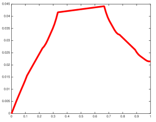
(a) Solution $p^{4}$, Stage $n=4$.

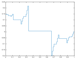
(b) Derivative $\bm{\partial}p^{4}$, Stage $n=4$.

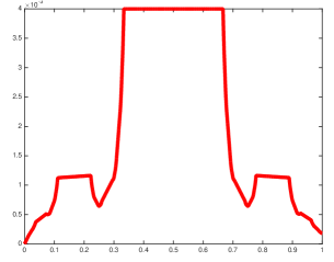
(c) Solution $p^{9}$, Stage $n=9$.

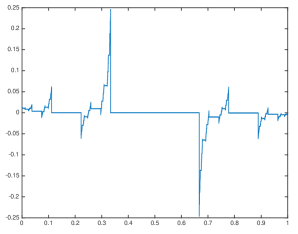
(d) Derivative $\bm{\partial}p^{9}$, Stage $n=9$.

Figure 1: Solutions Example 14. Storage coefficient $\beta=1$, forcing term $F=0$ and interface forcing term $f$, defined in Equation (32). The functions depicted in figures (a) and (c) are respectively, the solutions when the microstructures $\mathfrak{B}_{4}$ and $\mathfrak{B}_{9}$ are present; see (31). Figures (b) and (d) are the corresponding derivatives. The vertical lines in the derivatives’ graphics are included for optical purposes only.

Example 15 (Scaled Example)

In the second example we implement the model introduced in Section 3, in order to illustrate the behavior of the solutions. We set $F=0$, $f$ defined in Equation(32) above and the storage coefficient

$$\beta(\mathfrak{b})\overset{\mathbf{def}}{=}\sum_{n\,\in\,\bm{\mathbbm{N}}}\big{(}\frac{2}{3}\big{)}^{n}\,\bm{\mathbbm{1}}_{\mathfrak{B}_{n}-\mathfrak{B}_{n-1}}(\mathfrak{b})\,.$$ (33)

Due to its fractal nature, the exact solution can not be described explicitly. Therefore, we only present the Cauchy behavior of the sequence of solutions in Table 2 below, together with the corresponding graphics of the solutions in Figure 2. Again, convergence of the solutions is observed, as concluded by the theoretical results of Section 3.

Stage $n$	$\#$ Nodes	$\|p_{n}-p_{n-1}\|_{L^{2}(0,1)}$	$\|p_{n}-p_{n-1}\|_{H^{1}(0,1)}$
6	$3^{6}+1$	0.002708076748262	0.005143218742685
7	$3^{7}+1$	0.001344770703905	0.002552130987523
8	$3^{8}+1$	0.000670086347099	0.001271522606439
9	$3^{9}+1$	0.000334472470474	0.000634665496467

Table 2: Example 15: Convergence Table, $\beta$ defined in Equation (33).

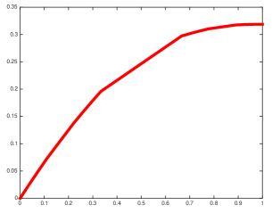
(a) Solution $p^{3}$, Stage $n=3$.

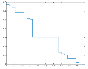
(b) Derivative $\bm{\partial}p^{3}$, Stage $n=3$.

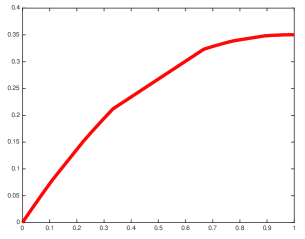
(c) Solution $p^{9}$, Stage $n=9$.

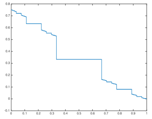
(d) Derivative $\bm{\partial}p^{9}$, Stage $n=9$.

Figure 2: Solutions Example 15. Storage coefficient $\beta$ defined in Equation (33), forcing term $F=0$ and interface forcing term $f$, defined in (32). The functions depicted in figures (a) and (c) are the corresponding solutions when the microstructures $\mathfrak{B}_{4}$ and $\mathfrak{B}_{9}$ are present, see (31). Figures (b) and (d) are the respective derivatives. The vertical lines in derivatives’ graphics are included for optical purposes only.

Example 16 (Random Behavior Example)

This third and last example is a probabilistic variation of Example 14. We simply introduce uncertainty in the storage coefficient $\beta$ by considering it a random variable, uniformly distributed on an interval i.e.,

$$\beta:\mathfrak{B}\rightarrow\Big{[}\frac{3}{4}\,,\frac{5}{4}\Big{]}\,, \beta\sim\text{uniformly}.$$ (34)

Due to the Law of Large Numbers, the average of $\beta$ is the constant function $\bar{\beta}=1$. Therefore, due to the linearity of the differential equation, the “averaged” function $\bar{p}$ of the solutions corresponding to the realizations is precisely the solution of Example 14. Below, Table 3 presents the results for eight numerical experiments, each of them consisting in averaging the outcome of twenty random realizations; we denoted this average by $\bar{p}_{n}$. The experiments were executed for two different stages, namely $n=4$ and $n=8$, consequently finite versions of the storage coefficient $\beta_{i}\overset{\mathbf{def}}{=}\beta\big{|}_{\mathfrak{B}_{i}}$ (introduced in(34)) were used, namely

$$\beta_{i}:\mathfrak{B}_{i}\rightarrow\Big{[}\frac{3}{4}\,,\frac{5}{4}\Big{]}\,, \beta_{i}\sim\text{uniformly}\,, i=4,8.$$ (35)

	Stage $n=4$		Stage $n=8$
Experiment	$\|\,\bar{p}_{n}-\bar{p}\,\|_{L^{2}(0,1)}$	$\|\,\bar{p}_{n}-\bar{p}\,\|_{H^{1}(0,1)}$	$\|\,\bar{p}_{n}-\bar{p}\,\|_{L^{2}(0,1)}$	$\|\,\bar{p}_{n}-\bar{p}\,\|_{H^{1}(0,1)}$
1	0.000119184000335	0.001061092385691	0.000003969114134	0.000255622745433
2	0.000212826056946	0.001524984778876	0.000011927845271	0.000729152212225
3	0.000251807786501	0.002145242883204	0.000006707500555	0.000433471661184
4	0.000118807313682	0.001071251072221	0.000006848283589	0.000399676826771
5	0.000200559658088	0.001539679789493	0.000003353682741	0.000236079667248
6	0.000274728964017	0.001805225518962	0.000017705174519	0.001055292921996
7	0.000262099625343	0.001921561839120	0.000013849036017	0.000696257848189
8	0.000338584909360	0.001974469520292	0.000004372910306	0.000289302820258
Average	0.000250408088105	0.001817080230904	0.000008011140143	0.000473741408661
Variance	$0.005804534\times 10^{-6}$	$0.164983904\times 10^{-6}$	$0.000027860\times 10^{-6}$	$0.083787371\times 10^{-6}$

Table 3: Example 16: Experiments, Each Consisting of 20 Random Realizations.

In the table 3 below, the $L^{2}$ and $H^{1}$-norms for the difference of the partial averages $\bar{p}_{n}$ and the Cesàro average are displayed. Clearly, convergence is observed in both cases and, due to the Law of Large Numbers, better behavior is observed at the stage $n=8$ over the stage $n=4$, as expected. The average and variance are also presented at the bottom of Table 3, which shows better behavior for the more developed stage $n=8$ over the stage $n=4$, not only in terms of centrality, but also in terms of deviation.

Finally, the solutions for some realizations are presented in Figure 3, where the microstructure is $\mathfrak{B}_{6}$. Clearly, the random realizations’ solutions are similarly shaped to its average value as expected.

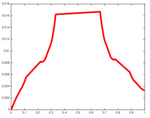
(a) Realization 1: Solution $p^{6}$.

(b) Realization 1: Derivative of the Solution $\bm{\partial}p^{6}$.

(c) Realization 2: Solution $p^{6}$.

(d) Realization 2: Derivative of the Solution $\bm{\partial}p^{6}$.

(e) Realization 3: Solution $p^{6}$.

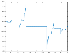
(f) Realization 3: Derivative of the Solution $\bm{\partial}p^{6}$.

Figure 3: Random Realizations Example 16. Storage coefficient $\beta$ defined in Equation(33), forcing term $F=0$ and interface forcing term $f$ defined in (32). For three random realizations, the functions depicted in figures (a), (c) and (e) are the solutions and figures (b), (d) and (f) are the corresponding derivatives. The microstructure is $\mathfrak{B}_{6}$, see Equation (31). The vertical lines in the derivatives’ graphics are included for optical purposes only.

4.3 Closing Observations

1. The Authors tried to find experimentally, a rate of convergence of the type $\|p^{n+1}_{i}-p^{n}_{i}\|=\mathcal{O}\big{(}\|p^{n}_{i}-p^{n-1}_{i}\|^{t_{i}}\big{)}$, $i=1,2$, using the well-know estimate

   $$t_{i}\sim\frac{\log\|p^{\,n+1}_{i}-p^{\,n}_{i}\|-\log\|p^{\,n}_{i}-p^{\,n-1}_{i}\|}{\log\|p^{\,n}_{i}-p^{\,n-1}_{i}\|-\log\|p^{\,n-1}_{i}-p^{\,n-2}_{i}\|}\,, i=1,2.$$

   The sampling was made on the sequence of stages $3,4,5,6,7,8,9$; experiments were run for Examples 14 and 15. However, in both cases, no solid numerical evidence suggesting an order of convergence for the phenomenon was detected.

2. Additional experiments for the Random Behavior Example 16 were executed. The probabilistic variations involved were

   1. Experiments for the stages $n=3,5,6,7$ and $9$.

   2. Experiments with different number of realizations, namely $20$, $60$ and $80$, depending on the computational time demanded.

   3. Using a storage coefficient $\beta:\mathfrak{B}\rightarrow I$, with different range intervals $I$ as well as uniform and normal distributions for $\beta$.

   4. Probabilistic variations of the forcing terms.

   5. Combinations of one or more of the previous factors.

   6. Execution of the aforementioned probabilistic variations adjusted to the scaled Example 15.

   In all the cases, convergence behavior was observed as expected. Naturally, the quality of convergence deteriorates depending on the deviation of the distributions as well as the combination of uncertainty factors introduced in the experiment.

3. All of the previously mentioned scenarios were also executed in the same code for the case of homogeneous Dirichlet boundary conditions on both ends i.e., $p_{n}(0)=p_{n}(1)=0$. As expected convergence behavior is observed, comparable with the corresponding analogous version used along the analysis of this paper i.e., Dirichlet-Neumann boundary conditions $p_{n}(0)=0$, $\bm{\partial}p_{n}(1)=0$.

5 Conclusions and Final Discussion

The present work yields several accomplishments as well as limitations listed below.

1. The unscaled storage model presented in Section 2 is in general not adequate, as it excludes most of the important cases of fractals.

2. The scaled storage model presented in Section 3 is suitable for an important number of fractal microstructures. However, the asymptotic variational model (27) is equivalent to a pointwise strong model (30), only if the closure of the microstructure $\operatorname*{cl}(\mathfrak{B})$ is negligible i.e., if it has null Lebesgue measure. Such hypothesis excludes important cases, e.g. the family of “fat” Cantor sets in 1-D or the “fat” versions of the classic fractal structures in 2-D and/or 3-D (see [14]). In these cases, only the “averaged normal flux” Statement (30d) can be concluded for the accumulation points of the microstructure $\mathfrak{B}^{\prime}$.

3. In order to overcome the deficiency previously mentioned, a first approach would be to take the traditional treatment of solving strong forms in fractal domains (as in [11, 13]) and then, try to “blend” it with the point of view presented here. Such analysis is to be pursued in future research.

4. The fractal microstructures addressed in this work are self-similar. This requirement is important only for the second model (Section 3) because it scales the storage coefficient $\beta$ (Equation (25)), according to the geometric detail of the structure at every level. In particular, in order to scale the storage coefficient adequately, accurate estimates of the growth rate of the microstructure $\mathfrak{B}$ from one level to the next are needed.

5. The self-similarity requirement for the microstructure $\mathfrak{B}$ in the introduction of the scaled model excludes the important family of the self-affine fractals; this type of microstructures is a topic for future work. On the other hand, the unscaled model of Section 2 does not require such detailed knowledge of the microstructure because it avoids scaling. Although it is likely to be unsuited for the analysis of self-affine microstructures it may be a good starting point, when looking for the needs to model this case.

6. It is important to observe the relevance of self-similarity versus the fractal dimension in the scaled model. While the self-similarity of the microstructure is the corner stone of the storage coefficient scaling, introduced in Equation (25) (hence, it can not be given up), the model is more flexible with respect to the fractal dimension of $\mathfrak{B}$, as long as it is not the same of the “host” domain $\Omega$.

7. We stress that the input needed by the present result, in terms of geometric information on the fractal structure, does not have to be as detailed as in the strong forms PDE analysis on fractals.

8. The random experiments presented in Example 16, as well as those only mentioned in Subsection 4.3, furnish solid numerical evidence of good behavior for probabilistic versions of the unscaled and the scaled models respectively. Additionally, it is important to handle certain level of uncertainty because, having a deterministic description of the fractal microstructure is a very strong hypothesis to be applicable in realistic scenarios. In the Authors’ opinion, this is justification enough to pursue rigorous analysis of these problems, which will be addressed in future work.

9. In Example 16, uncertainty was introduced in the storage coefficient $\beta$, or the forcing term $f$, however the geometry of the microstructure was never randomized. In several works (e.g. [17, 18]) the self-similarity is replaced by the concept of statistical self-similarity, in the sense that scaling of small parts have the same statistical distribution as the whole set. Clearly, this random property is consistent with the scaling of $\beta$ (25) in Definition 5. Consequently, the statistical self-similarity is a future line of research, in order to address geometric uncertainty of the fractal microstructure $\mathfrak{B}$. In particular, the fractal percolation microstructures, are of special interest for real world applications, see [19, 20].

10. The execution of all the numerical experiments shows that the code becomes unstable beyond the 9th stage of the Cantor set construction. This suggests that in order to overcome these limitations, an adaptation of the FEM method has to be developed, targeted to the microstructure of interest. This aspect is to be analyzed in future research.

11. The study of fractal microstructures in 2-D and 3-D are necessary for practical applications and in higher dimensions for theoretical purposes. Since passing from one dimension to two or more dimensions, increases significantly the level of complexity in the microstructure and in the equation, considerable challenges are to be expected in this future research line.

12. Another important analysis to be developed is the study of the models both, scaled and unscaled, in the mixed-mixed variational formulation introduced in [21]. On one hand, this approach allows great flexibility for the underlying spaces of velocity and pressure, which can constitute an advantage with respect to the treatment presented here. On the other hand, the mixed-mixed variational formulation allows modeling fluid exchange conditions across the interface of greater generality than the conditions in (8b), used in the present work; this advantage can contribute significantly to the development of the field.

References

• [1] R. Showalter, Distributed microstructure models of porous media, Flow in porous media. Proceeding of the Oberwolfach Conference 114, No 3 (1993) 155–163.
• [2] R. Showalter, N. Walkington, A diffusion system for fluid in fractured media, Differential & Integral Equations 3 (1990) 219–236.
• [3] R. Showalter, N. Walkington, Diffusion of fluid in a fissured medium with microstructure, SIAM J. Math. Anal. 22, No 6 (1991) 1702–1722.
• [4] T. Arbogast, D. Brunson, A computational method for approximating a Darcy-Stokes system governing a vuggy porous medium, Computational Geosciences 11, No 3 (2007) 207–218.
• [5] T. Arbogast, H. Lehr, Homogenization of a Darcy-Stokes system modeling vuggy porous media, Computational Geosciences 10, No 3 (2006) 291–302.
• [6] F. A. Morales, Homogenization of geological fissured systems with curved non-periodic cracks, Electronic Journal of Differential Equations 2014 No. 189 (2014) 1–21.
• [7] A. Katz, A. Thompson, Fractal sandstone pores: Implications for conductivity and pore formation, Physical Review Letters 54(12) (1985) 1325.
• [8] J. Zheng, X. Shi, J. Shi, Z. Chen, Pore structure reconstruction and moisture migration in porous media, Fractals 22 No3 (2014) 1440007, 1–9.
• [9] J. Feder, T. Jøssang, Fractal flow in porous media, Physica Scripta T29 (1989) 200–205.
• [10] L. Zhang, J. Li, H. Tang, J. Guo, Fractal pore structure model and multilayer fractal adsorption in shale, Fractals 22 No3 (2014) 14400010, 1–12.
• [11] R. S. Strichartz, Sovability for differential equations on fractals, Journal of Funcional Analysis 96 (2005) 247–267.
• [12] M. T. Barlow, J. Kigami, Localized eigenfunctions of the Laplacian on p.c.f. self-similar sets, Journal of the London Mathematical Society 56(2) (1997) 320–332.
• [13] R. S. Strichartz, Function spaces on fractals, Journal of Funcional Analysis 198 (2003) 43–83.
• [14] K. Falconer, Fractal Geometry: Mathematical Foundations and Applications. Second Edition, John Wiley $\&$ Sons, 2003.
• [15] R. E. Showalter, Hilbert space methods for partial differential equations, Vol. 1 of Monographs and Studies in Mathematics, Pitman, London-San Francisco, CA-Melbourne, 1977.
• [16] M. Peszyńska, fem1d.m: Template for solving a two point boundary value problem, Library, http://www.math.oregonstate.edu/~mpesz/code/teaching.html (2008–2015).
• [17] S. Graf, Statistically self-similar fractals, Probability Theory and Related Fields 74, No 3 (1987) 357–395.
• [18] J. E. Hutchinson, L. Rüschendorf, Random fractals and probability metrics, Advances in Applied Probability 32, No 4 (2000) 925–947.
• [19] J. T. Chayes, L. Chayes, R. Durret, Connectivity properties of Mandelbrot’s percolation process, Probability Theory and Related Fields 77, No 3 (1988) 307–324.
• [20] F. M. Dekking, R. W. J. Meester, On the structure of Mandelbrot’s percolation process and other random cantor sets, Journal of Statistical Physics 58, No 5/6 (1990) 1009–1126.
• [21] F. Morales, R. Showalter, Interface approximation of Darcy flow in a narrow channel, Mathematical Methods in the Applied Sciences 35 (2012) 182–195.