The K2-ESPRINT Project III: A Close-in Super-Earth around a Metal-rich Mid-M Dwarf

Abstract

We validate a $R_{p}=2.32\pm 0.24R_{\oplus}$ planet on a close-in orbit ($P=2.260455\pm 0.000041$ days) around K2-28 (EPIC 206318379), a metal-rich M4-type dwarf in the Campaign 3 field of the K2 mission. Our follow-up observations included multi-band transit observations from the optical to the near infrared, low-resolution spectroscopy, and high-resolution adaptive-optics (AO) imaging. We perform a global fit to all the observed transits using a Gaussian process-based method and show that the transit depths in all passbands adopted for the ground-based transit follow-ups ($r^{\prime}_{2},z_{\mathrm{s,2}},J,H,K_{\mathrm{s}}$) are within $\sim 2\sigma$ of the K2 value. Based on a model of the background stellar population and the absence of nearby sources in our AO imaging, we estimate the probability that a background eclipsing binary could cause a false positive to be $<2\times 10^{-5}$. We also show that K2-28 cannot have a physically associated companion of stellar type later than M4, based on the measurement of almost identical transit depths in multiple passbands. There is a low probability for a M4 dwarf companion ($\approx 0.072_{-0.04}^{+0.02}$), but even if this were the case, the size of K2-28b falls within the planetary regime. K2-28b has the same radius (within $1\sigma$) and experiences a similar irradiation from its host star as the well-studied GJ 1214b. Given the relative brightness of K2-28 in the near infrared ($m_{\mathrm{Kep}}=14.85$ mag and $m_{H}=11.03$ mag) and relatively deep transit ($0.6-0.7\%$), a comparison between the atmospheric properties of these two planets with future observations would be especially interesting.

1. Introduction

With relatively low masses and small physical sizes, M dwarfs are attractive targets for the search and characterization of small planets. GJ 1214b is one of the most intensely observed exoplanets, and the first detailed atmospheric characterization of this intermediate-sized planet between Earth- and Neptune-like ones was enabled by the large transit depth and brightness of its host star (e.g., Charbonneau et al., 2009; Bean et al., 2010; Kreidberg et al., 2014). However, both the census of small planets around mid-to-late M dwarfs (stars with effective temperatures of $T_{\mathrm{eff}}\leq 3400$ K) and the atmospheric characterization of these objects are still in their infancy; only five transiting systems (GJ 1214, GJ 1132, Kepler-42, Kepler-445, and Kepler-446) have been reported to date around mid-to-late M dwarfs (Muirhead et al., 2012, 2015; Berta-Thompson et al., 2015), and the latter three are too faint or the transit depths too shallow to permit intensive follow-up studies.

The failure of a second reaction wheel ended the Kepler prime mission, but the spacecraft’s second mission (“K2”) consists of observations of new fields and new targets with a cycle of $\sim 80$ days (Howell et al., 2014). K2 has so far unveiled many planetary systems with distinguishing characteristics, including a compact multi-planet system with sub-Saturn-mass planets in the 3:2 mean motion resonance (Armstrong et al., 2015), multiple systems with Earth- to super-Earth-sized planets around rather bright M dwarfs (Crossfield et al., 2015; Petigura et al., 2015), and a disintegrating minor planet around a white dwarf (Vanderburg et al., 2015). In order to fully exploit the worldwide ground facilities for K2 follow-ups, we had started the ESPRINT (Equipo de Seguimiento de Planetas Rocosos Intepretando sus Transitos) collaboration, which aims to discover and characterize unique transiting planets unveiled by K2. ESPRINT has contributed to the K2 haul of discoveries with a disintegrating ultra-short period planet with a cometary tail around an M dwarf (ESPRINT I: Sanchis-Ojeda et al., 2015), and confirmation of three systems in the Campaign 1 field by radial velocity measurements (ESPRINT II: Van Eylen et al., 2016).

In this paper we validate a $R_{p}=2.32R_{E}$ planet around a mid-M star in K2 Campaign 3, which is located at a high galactic latitude ($+60^{\circ}$) and samples a distinct stellar population from the prime Kepler mission. Our target is labeled as EPIC 206318379 (which we call K2-28 hereafter) with the Kepler magnitude of $m_{\mathrm{Kep}}=14.854$. The relative brightness of the star in the near infrared (e.g., $m_{H}=11.03$) summarized in Table 1 from the SDSS (Ahn et al., 2012) and 2MASS (Skrutskie et al., 2006) catalogs suggest that it is a rather cool star ($T_{\mathrm{eff}}\sim 3000$ K) and thus an excellent target for further follow-up studies.

We organize the rest of the paper as follows. In Section 2, we describe how we reduced and detected the planet candidates in K2 field 3, and present the ground-based observations for the target, including follow-up transit observations with the Infrared Survey Facility (IRSF) 1.4-m telescope and Okayama 1.88-m telescope, low-resolution spectroscopy with UH88 and the NASA Infrared Telescope Facility (IRTF), and adaptive-optics (AO) imaging with the Subaru 8.2-m telescope. We then carefully analyze the ground and space-based transit observations in Section 3 using Gaussian processes. The transit depths from the ground-based follow-ups are compared to that from the K2 reduced light curve, and consequently we show that they are all in agreement within $\sim 2\sigma$. Section 4 describes to what extent we are able to exclude the false positive scenario by first computing the probability that the transit-like signal is caused by a background eclipsing binary, which turns out to be very low ($\approx 2\times 10^{-5}$). The almost constant transit depths from the optical to the near infrared also put a constraint on the magnitude of possible close-in companion around K2-28. Finally, Section 5 is devoted to discussion and summary.

2. Observations and Data Reductions

2.1. K2 Photometry

The images of all the K2 Campaign 3 targets were downloaded from MAST, and we used our own tools (described in detail in Sanchis-Ojeda et al., 2015) to produce corrected light curves ready for our planet search routines. In particular, field 3 targets were observed for 69 days, from 2014 November 15 through 2015 January 23. The dataset was split into 9 segments with a duration of approximately 7.5 days each. Because of the faintness of K2-28, we defined an aperture at each segment with all the pixels that had 4% more counts than the mean background on at least 50% of the images of that segment. The light curves are corrected both for instrumental noise induced by the motion of the telescope and astrophysical long term variability using independent 4th-order polynomials with both time and centroid motion as variables.

We searched the processed long cadence light curves in K2 Campaign 3 for planet candidates using a Box-fitting Least Squares routine (BLS: Kovács et al., 2002; Jenkins et al., 2010). We improved the efficiency of the original BLS by implementing the optimal frequency sampling described in Ofir (2014). K2-28 emerged as a clear detection with SNR of $\sim$9. A linear ephemeris analysis gave a best-fit period of $P=2.26023\pm 0.00012$ days and mid-transit time of $T_{c,0}=2456977.9924\pm 0.0021$.

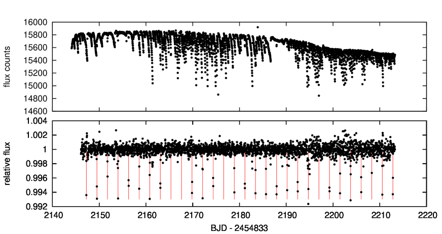
Figure 1.— Full light curves for K2-28 obtained by our custom-made aperture. (Top) Raw light curve. (Bottom) Reduced light curve after the correction for the centroid motion and flux baseline variations. The equally-spaced red vertical lines corresponds to the transits of K2-28b.

In the archived SDSS image of K2-28 there is a second, fainter ($\Delta m_{r}=4.802\pm 0.035$ mag) source $\sim 5\farcs 2$ to the north-east. We made sure that given the difference in magnitude, there is no excess of brightness detected in the K2 data pixels around the location of the faint companion seen in the SDSS image. Our imaging and astrometric analysis show the fainter source to have proper motion with respect to K2-28 and is thus physically unrelated and probably a background star (Section 4.1). We determined the position of the star at the epoch of K2 observations, designed a K2 photometric aperture that excludes this star but includes the 8 brightest pixels for K2-28  and extract a light curve using this aperture and the public code outlined in Van Eylen et al. (2016). Figure 1 shows thus extracted light curves with and without the correction for the centroid motions and baseline flux variations. Some of the data points, including ones during transits, are missing in the reduced light curve (bottom), mainly due to the removal of outliers when we corrected for the centroid motion and baseline function. The revised light curve contains the same transit events with the same depth, suggesting that K2-28 and not the fainter star is the source of the signal.

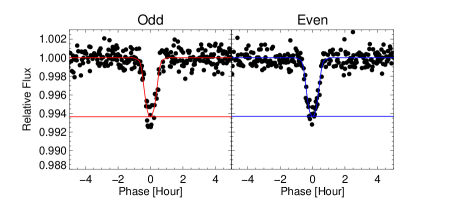
Figure 2.— Folded light curves during the odd (left) and even (right) transits.

We also performed an odd-even test by folding the K2 light curve with twice the period of K2-28 b. As shown in Figure 2, the odd and even transits exhibit equal depths within $0.08\sigma$, where $\sigma$ is defined as the depth uncertainty for each folded transit in the preliminary depth measurement, indicating that we have identified the correct period. The odd-even test also shows no indication of a secondary eclipse, excluding many false-positive scenarios involving an eclipsing binary. We therefore conducted a campaign of follow-up observations to validate this candidate planet.

2.2. Follow-up Transit Observations

2.2.1 IRSF 1.4 m/SIRIUS

We conducted a follow-up transit observation with the Simultaneous Infrared Imager for Unbiased Survey (SIRIUS; Nagayama et al., 2003) mounted on the IRSF 1.4-m telescope at South African Astronomical Observatory on 2015 August 7 UT. SIRIUS has three infrared detectors, each having 1,024 $\times$ 1,024 pixels with the pixel scale of 0$\farcs$45 pixel^-1, allowing $J$-, $H$-, and $K_{\mathrm{s}}$-band simultaneous imaging. The exposure times were set to 30 s for all bands. We started the observation at 20:50 UT and continued it until 24:03 UT (the airmass had changed from 1.54 to 1.10), covering the expected duration of a transit. During the SIRIUS observation, we employed the position-locking software to fix the centroid of stellar images within a few pixels from the initial position (Narita et al., 2013a, b).

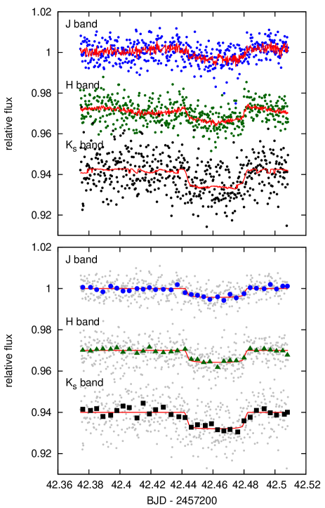
Figure 3.— (Top) K2-28’s raw light curves by IRSF/SIRIUS. The GP regression to each dataset is shown by the red line. (Bottom) Reduced light curves (grey points) after subtracting the GP regressions to correlated noises. The blue, green, and black symbols indicate 16-point binned fluxes for the $J$, $H$, $K_{s}$ bands, respectively. The best-fit transit model for each band is shown by the red solid line. Light curves in different bands have a vertical offset for clarity.

The observed images were bias-subtracted and flat-fielded in the standard manner. For the flat fielding, we combined 15, 18, and 17 twilight flat images for $J$, $H$, and $K_{\mathrm{s}}$ bands, respectively, taken before and after the observation. We then performed aperture photometry using two, one, and one comparison star(s) for $J$, $H$, and $K_{\mathrm{s}}$, respectively, by using a custom code (Fukui et al., 2011). The aperture sizes of 6.0, 8.0, and 6.0 pixels were selected for the $J$-, $H$-, and $K_{\mathrm{s}}$-band data to minimize the dispersion of the light curves with respect to the best-fit transit models. The time system of the light curves was converted from Julian Day (JD) to Barycentric JD (BJD) by the code of Eastman et al. (2010). The resulting light curves are plotted in the top panel of Figure 3.

2.2.2 OAO 188 cm/MuSCAT

We also conducted a follow-up transit observation with the Multicolor Simultaneous Camera for studying Atmospheres of Transiting exoplanets (MuSCAT; Narita et al., 2015) mounted on the 188-cm telescope at Okayama Astrophysical Observatory (OAO) on 2015 August 23 UT. MuSCAT consists of three CCDs, each having 1,024 $\times$ 1,024 pixels with the pixel scale of 0$\farcs$36 pixel^-1, allowing simultaneous three-band imaging through the Generation 2 Sloan $g^{\prime}_{2}$-, $r^{\prime}_{2}$-, and $z_{\mathrm{s,2}}$-band filters. MuSCAT can also fix the centroid of stellar images within $\sim 1$ pixel from the initial position (Narita et al., 2015). Because the $g^{\prime}_{2}$-band channel was not available at that time due to an instrumental trouble, we used the remaining two channels for the observation. The exposure times were set to 120 s and 60 s for the $r^{\prime}_{2}$ and $z_{\mathrm{s,2}}$ bands, respectively. We started the observation at 17:10 UT and continued it until 18:48 UT (the airmass had changed from 1.54 to 2.33), covering the first half of the transit.

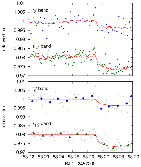
Figure 4.— (Top) K2-28’s raw light curves by OAO/MuSCAT. The GP regression to each dataset is shown by the red line. (Bottom) Reduced light curves (grey points) after subtracting the GP regressions to correlated noises. The blue and green symbols indicate 4-point and 8-point binned fluxes for the $r^{\prime}_{2}$ and $z_{\mathrm{s,2}}$ bands, respectively. The best-fit transit model for each band is shown by the red solid line. Light curves in different bands have a vertical offset for clarity.

The observed images were reduced by the same procedure as done in Section 2.2.1. For the flat fields, we used one hundred dome-flat images taken on the same observing night for all bands. We performed the aperture photometry using three comparison stars for all bands, with the aperture sizes of 18 pixels for both of the $r^{\prime}_{2}$- and $z_{\mathrm{s,2}}$-band data. The produced light curves are shown in the top panel of Figure 4.

We note that the comparison stars of our ground-based photometry are all solar-type ones with their colors ranging from $V-J=1.2$ to $2.4$, which are in stark contrast to the color of K2-28 ($V-J=4.37$). This difference could be a source of systematic effects in the reduced light curves arising from relative flux variations by e.g., changing precipitable water vapor and target’s airmass. But the five photometric bands that we employed are generally less affected by the telluric water absorption, and in particular, the $z_{\mathrm{s,2}}$-band is designed to avoid strong telluric absorption. The target’s airmass was changing monotonically during the IRSF and OAO runs, and thus its impact is not expected to be large as long as the baseline of the light curve is corrected from the out-of-transit flux data.

2.3. Optical Low Resolution Spectroscopy

We obtained an optical spectrum of K2-28 with the SuperNova Integral Field Spectrograph (SNIFS Lantz et al., 2004) on the UH88 telescope on Mauna Kea during the night of August 9, 2015 (UT). SNIFS provides spectra covering 3200 to 9700 Å at a resolution of $\lambda/\Delta\lambda=700-1000$. Full details on data reduction can be found in Aldering et al. (2002) and Mann et al. (2013b). The resulting spectrophotometric calibration of SNIFS spectra has been shown to be good to 2-3% (Mann et al., 2013b), which is sufficient to establish fundamental stellar parameters of M dwarfs.

Table 1Stellar Parameters of K2-28 (EPIC 206318379)

Parameter	Value
(Stellar Parameters from the SDSS and 2MASS Catalogs)
RA	$22:22:29.88$
Dec	$-07:57:19.55$
$\mu_{\alpha}$ (mas yr-1)	$-256\pm 3$
$\mu_{\delta}$ (mas yr-1)	$-195\pm 3$
$m_{g}$ (mag)	$16.839\pm 0.004$
$m_{r}$ (mag)	$15.449\pm 0.004$
$m_{i}$ (mag)	$13.909\pm 0.003$
$m_{z}$ (mag)	$13.103\pm 0.003$
$m_{J}$ (mag)	$11.70\pm 0.03$
$m_{H}$ (mag)	$11.03\pm 0.02$
$m_{K_{\mathrm{s}}}$ (mag)	$10.75\pm 0.02$
(Spectroscopic and Derived Parameters)
$T_{\rm eff}$ (K)	$3214\pm 60$
$[\mathrm{Fe/H}]$ (dex)	$0.26\pm 0.10$
$\log g$ (dex)	$4.93\pm 0.04$
$R_{\star}$ ($R_{\odot}$)	$0.288\pm 0.028$
$M_{\star}$ ($M_{\odot}$)	$0.257\pm 0.048$
$\rho_{\star}$ ($\rho_{\odot}$)	$10.8\pm 2.4$
distance (pc)	$53\pm 8$

We derived the effective temperature following the procedure from Mann et al. (2013b). To briefly summarize, we compare our optical spectrum to BT-SETTL models (Allard et al., 2013) calibrated to reproduce the temperatures of nearby stars with radii and temperatures measured from long-baseline interferometry (Boyajian et al., 2012). This method yielded $T_{\rm{eff}}=3214\pm 60$ K.

2.4. Near Infrared Spectroscopy

We obtained a near-infrared (NIR) spectrum of K2-28 with the updated SpeX spectrograph (Rayner et al., 2003) mounted on IRTF on Mauna Kea. SpeX observations were taken with the 0.3$\times 15\arcsec$ slit in the cross-dispersed mode, which provides simultaneous coverage from 0.8 to 2.4$\mu$m at $R\simeq 2000$. We placed the target at two positions along the slit (A and B) and observed in an ABBA pattern in order to subsequently subtract the sky background. In total we took six exposures following this pattern, which when stacked, yielded a S/N per pixel of 65 in the $H$ and $K$ bands. To correct for telluric lines, an A-type star was observed immediately after the target observations with much higher S/N ($>100$).

SpeX spectra were extracted using the SpeXTool package (Cushing et al., 2004), which includes flat-field correction, wavelength calibration, sky subtraction, and extraction of the one-dimensional spectrum. Multiple exposures were combined using the IDL code xcombspec. A telluric correction spectrum was constructed from the A0V star and applied using the xtellcor package (Vacca et al., 2003).

Metallicity was calculated from the IRTF spectrum utilizing procedure from Mann et al. (2013a). Mann et al. (2013a) provides empirical relations between spectroscopic feature strength and metallicity calibrated against wide binaries containing a solar-type star and an M dwarf. We used the mean of the $H$ and $K$ band relations, accounting for both Poisson and calibration errors. This method gave a metallicity of $[\mathrm{Fe/H}]=0.26\pm 0.10$. With $T_{\rm{eff}}$ derived from the optical spectrum and $[\mathrm{Fe/H}]$ from the NIR spectrum, we computed the stellar radius and mass following the empirical relations from Mann et al. (2015). These values are reported in Table 1 along with other derived parameters (i.e., the stellar density $\rho_{\star}$, surface gravity $\log g$, and distance to the star).

2.5. AO Imaging

We conducted a high-angular resolution imaging with the Subaru telescope equipped with the adaptive optics (AO) instrument AO188 and the Infrared Camera and Spectrograph (IRCS, Kobayashi et al. 2000) on 2015 September 17 UT. We used the “high-resolution” mode of IRCS, which has a pixel scale of 20.6 mas pixel^-1 and the FOV of 21$\farcs$1 $\times$ 21$\farcs$1. We used the target star itself as a natural guide star. The target star was observed through the $K^{\prime}$-band filter at nine dithering points, each with the exposure time of 30 s (2 s $\times$ 15 coadds), resulting in the total integration time of 270 s. The airmass was 1.26 and the AO-worked full width at half maximum (FWHM) of the target $\sim$0$\farcs$18.

The observed images were dark-subtracted and flat-fielded in a standard manner. Twilight flat images taken in the morning were used for the flat fielding. The reduced images were then aligned, sky-level-subtracted, and median-combined. The combined image and the 5-$\sigma$ contrast curve are shown in Figure 5.

3. Analyses of the Light Curves

Due to the sparse time sampling of the K2 data ($\sim 0.5$ hour) in comparison with the transit duration ($\sim 1$ hour), the folded K2 transit curve looks V-shaped as shown in Figure 6. This leads to a degeneracy in system parameters (i.e., the scaled semi-major axis $a/R_{s}$, transit impact parameter $b$, and planet-to-star radius ratio $R_{p}/R_{s}$) when we fit the time-integrated K2 flux data alone. On the other hand, the follow-up transit curves exhibit a clearer ingress (egress) and flat bottom (especially in the $z_{\mathrm{s,2}}$-band) in spite of the worse photometric precision than Kepler, suggesting that the transiting body is significantly smaller than the central late-type star. The clear ingress and egress also enable us to better constrain the transit parameters, and thus we here decide to fit the follow-up transit curves simultaneously with the K2 light curve.

When a source of dilution, i.e. a physical companion star or background star, is present in the photometric aperture, the transit depths measured in different bands may vary depending on the contrast ratio of the objects in each band. Conversely, a wavelength-independent transit depth is suggestive of no dilution source in the aperture, on the assumption that the diluting star does not have an identical spectral energy distribution as that of the primary. Thus, in order to constrain the presence of possible dilution sources, we attempt to measure the radius ratio for each observed band as accurately as possible, and compare the results in different bands from the optical to the near infrared. Since only a part of the transit is observed for OAO datasets, we do not attempt to fit the light curves in individual bands, but combine all the transit curves and perform a global fit.

We employ the method of Gaussian processes (GP) to obtain the most accurate radius ratio for each band from our current datasets. In addition to the flux counts, ground-based observations in general provide many auxiliary variables such as target’s pixel centroid drifts, sky background count, target’s FWHM in the photometric aperture, etc., which are not monotonic functions of time. Time-correlated noises are also present in our datasets owing both to the intrinsic stellar activity and other instrumental systematics. Taking account of these pieces of information in modeling the observed light curves yields more accurate estimates for the model parameters (e.g., Gibson et al., 2012). A GP model assumes that the observed flux values with $N_{\mathrm{data}}$ points follow a multi-variable Gaussian:

$$\mathcal{N}(\mathbf{\mu},\Sigma)=\frac{1}{\sqrt{(2\pi)^{N_{\mathrm{data}}}|\Sigma|}}\exp\left\{-\frac{(\mathbf{f}-\mathbf{\mu})^{\mathrm{T}}\Sigma^{-1}(\mathbf{f}-\mathbf{\mu})}{2}\right\},~{}~{}$$ (1)

where $\mathbf{f}$ and $\mathbf{\mu}$ are the observed and modeled flux vectors (with $N_{\mathrm{data}}$ components), and $\Sigma$ is the covariance matrix. When $\Sigma$ has only diagonal components, representing independent Gaussian noises in individual fluxes, the exponent in Equation (1) reduces to $-\chi^{2}/2$. By introducing non-diagonal components in the covariance matrix $\Sigma$, we can deal with correlated noises among flux values, not only as a function of time but also functions of other auxiliary parameters like pixel centroid shifts and sky background counts, which are often corrected by modeling the baseline flux variations with e.g., polynomials of the parameters. In a GP modeling, we do not need to assume such a functional form for the flux variation by auxiliary variables, and the best correlation pattern among the flux values are found in the fitting process through an optimization of hyper-parameters (Rasmussen & Williams, 2006).

We estimate the posterior distribution of the system parameter vector $\alpha$ using Bayes’ theorem:

$$p(\mathbf{\alpha}|\mathrm{data})\propto\mathcal{L}(\mathrm{data}|\mathbf{\alpha})\cdot p(\mathbf{\alpha}),$$ (2)

where $\mathcal{L}(\mathrm{data}|\mathbf{\alpha})$ is the likelihood of the flux values and $p(\mathbf{\alpha})$ is a prior distribution for the system parameters. In the present case, where we simultaneously model the observed fluxes in five different bands with GP, the likelihood $\mathcal{L}$ is expressed as a product of Gaussians given in Equation (1) for individual bands:

$$\ln\mathcal{L}(\mathrm{data}|\mathbf{\alpha},\mathbf{\theta}) = -\frac{1}{2}\sum_{i=r^{\prime}_{2},z_{\mathrm{s,2}},J,H,K_{\mathrm{s}}}\{(\Delta\mathbf{f}^{(i)})^{\mathrm{T}}(\Sigma^{(i)}(\mathbf{\theta}))^{-1}\Delta\mathbf{f}^{(i)}$$ (3)

$$+\ln|\Sigma^{(i)}(\theta))|+N_{\mathrm{data}}^{(i)}\ln(2\pi)\}$$

$$-\frac{1}{2}\chi_{\mathrm{K2}}^{2}+\mathrm{const.},$$

where $\Delta\mathbf{f}^{(i)}=\mathbf{f}^{(i)}-\mathbf{\mu}^{(i)}(\mathbf{\alpha})$, and $\mathbf{f}^{(i)}$ and $\mathbf{\mu}^{(i)}$ are $i-$th band’s observed and model flux vectors each comprised of $N_{\mathrm{data}}^{(i)}$ rows, and $\Sigma^{(i)}(\mathbf{\theta})$ is the covariance matrix of $N_{\mathrm{data}}^{(i)}\times N_{\mathrm{data}}^{(i)}$ for that dataset. The vectors $\mathbf{\alpha}$ and $\mathbf{\theta}=\{A_{j}^{(i)},L_{j}^{(i)}\}$ are transit model parameters and hyper-parameters, respectively, which are to be optimized by the procedure below. For the model flux $\mathbf{\mu}^{(i)}$, we use the analytic model by Ohta et al. (2009). Since we have already corrected for the pixel centroid motion and time-dependent flux variation in extracting the reduced K2 light curve, we employ a simple $\chi^{2}$ statistics for the K2 dataset as

$$\chi_{\mathrm{K2}}^{2}=\sum_{i}\frac{(f_{\mathrm{LC,obs}}^{(i)}-f_{\mathrm{LC,model}}^{(i)})^{2}}{\sigma_{\mathrm{LC}}^{(i)2}},$$ (4)

where $f_{\mathrm{LC,obs}}^{(i)}$ and $\sigma_{\mathrm{LC}}^{(i)}$ are the $i$-th observed K2 flux and its error, respectively. For $f_{\mathrm{LC,obs}}^{(i)}$, we extracted light curve segments only around the transit (covering $\pm 2$ times the transit duration from the mid-transit time) from the full reduced K2 light curve to save the computation time. Note that $f_{\mathrm{LC,model}}^{(i)}$ is computed by integrating the transit model flux (Ohta et al., 2009) over the cadence of K2 observation ($\sim 29.4$ minutes).

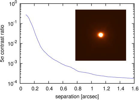
Figure 5.— $5\sigma$ Contrast curve around K2-28 based on the AO observation with Subaru/IRCS. The inset displays the combined image with the FOV of $3\farcs 2\times 3\farcs 2$. North is up and east is left.

For the covariance matrix $\Sigma$, there are some choices to describe the correlations between flux values and auxiliary parameters. Here we simply adopt the following combination of white noises and the “squared exponential” kernels:

$$\Sigma^{(i)}_{nm}=\sum_{j=1}^{5}A_{j}^{(i)2}\exp\left(-\frac{(p_{j,n}^{(i)}-p_{j,m}^{(i)})^{2}}{2L_{j}^{(i)2}}\right)+\delta_{nm}\sigma_{n}^{(i)2},$$ (5)

where the first term corresponds to the correlation between the input variables (parameters) $p_{j,n}^{(i)}$ and $p_{j,m}^{(i)}$, while the second term is the white noise component in each of the observed fluxes. As auxiliary variables $p_{j,n}^{(i)}$, we here employ the time $t$, $x$ and $y$ pixel centroid drifts (each), sky background count, and target’s FWHM in the photometric aperture, in total introducing ten hyper-parameters for each bandpass. In this specific covariance matrix, we can “learn” from the data the amplitude and length (scale) of the flux correlation as a function of each auxiliary variables by optimizing the hyper-parameters $A_{j}^{(i)}$ and $L_{j}^{(i)}$. We do not incorporate the target’s airmass as an auxiliary parameter, since target’s airmass varied monotonically against time during both IRSF and OAO runs, implying that GP regressions by target’s airmass could be degenerate with those by time (red noise). As we show in Section 5, however, fitting the light curves including airmass terms in the GP regression yields a fully consistent result with the one without airmass terms.

Table 2Result of the Global Fit to Transit Light Curves

Parameter	$r^{\prime}_{2}$-band	$z_{\mathrm{s,2}}$-band	$J$-band	$H$-band	$K_{\mathrm{s}}$-band	Kepler-band
(Fitting Parameters in individual bands)
$u_{1}+u_{2}$	$0.78\pm 0.10$	$0.64\pm 0.10$	$0.45\pm 0.10$	$0.44\pm 0.10$	$0.34\pm 0.10$	$0.080\pm 0.09$
$u_{1}-u_{2}$	$0.13\pm 0.10$	$0.43\pm 0.10$	$-0.29\pm 0.10$	$-0.32\pm 0.10$	$-0.28\pm 0.10$	$0.00\pm 0.10$
$R_{p}/R_{s}$	$0.056_{-0.010}^{+0.009}$	$0.077_{-0.004}^{+0.005}$	$0.063\pm 0.007$	$0.073\pm 0.007$	$0.086_{-0.006}^{+0.005}$	$0.0737_{-0.0018}^{+0.0032}$
(Common Fitting Parameters)
$a/R_{s}$	$17.9_{-2.8}^{+1.2}$
$b$	$0.36_{-0.24}^{+0.26}$
$e$	$0$ (fixed)
$P$ (days)	$2.260455\pm 0.000041$
$T_{c}^{\mathrm{(IRSF)}}$			$2457242.4620_{-0.0048}^{+0.0049}$
$T_{c}^{\mathrm{(OAO)}}$	$2457258.2849_{-0.0051}^{+0.0052}$
$T_{c}^{\mathrm{(K2)}}$						$2456977.99012_{-0.00074}^{+0.00075}$

In the global fit to the light curves, we have the following system model parameters: $a/R_{s}$, $b$, $P$, the limb-darkening parameters $u_{1}$ and $u_{2}$ for the quadratic limb-darkening law, $R_{p}/R_{s}$, and times of mid-transit for OAO, IRSF, and K2 datasets ($T_{c}^{\mathrm{(OAO)}}$, $T_{c}^{\mathrm{(IRSF)}}$, and $T_{c}^{\mathrm{(K2)}}$) as summarized in Table 2. Among these, $a/R_{s}$, $b$, $P$, $T_{c}^{\mathrm{(OAO)}}$, $T_{c}^{\mathrm{(IRSF)}}$, $T_{c}^{\mathrm{(K2)}}$ are common to all datasets, but we allow the other parameters to vary to see the possible variation in $R_{p}/R_{s}$ for each band. Due to the quality of the data, we are forced to fix the orbital eccentricity at zero, and also impose Gaussian priors (with dispersions of $0.1$ for both $u_{1}+u_{2}$ and $u_{1}-u_{2}$) on the limb-darkening parameters based on the table provided by Claret et al. (2013) as $p(\mathbf{\alpha})$ in Equation (2). To take into account the case that the internally estimated white noise for each flux value ($\sigma_{n,\mathrm{internal}}^{(i)}$: photon plus scintillation noise) is underestimated, we also optimize the white noise component $\sigma_{n}^{(i)}$ in Equation (5) by introducing additional free parameters $\sigma_{\mathrm{white}}^{(i)}$ for individual bands via

$$\sigma_{n}^{(i)}=\sqrt{\sigma_{n,\mathrm{internal}}^{(i)2}+\sigma_{\mathrm{white}}^{(i)2}}.$$ (6)

On the basis of Bayesian framework, we estimate the marginalized posteriors for those parameters. Ideally, the posterior distributions for these fitting parameters should be inferred by marginalizing all of the system and hyper-parameters. But the size of data and the huge number of parameters prohibit the full marginalization: computation of the inverse covariance matrix is rather expensive. Therefore, following Evans et al. (2015), we decide to adopt the so-called type-II maximum likelihood as below. We first maximize Equation (3) by the Nelder-Mead simplex method (e.g., Press et al., 2002), varying all the model and hyper-parameters. We then fix the hyper-parameters and $\sigma_{\mathrm{white}}^{(i)}$ in Equation (6) at the optimized values, and run Markov Chain Monte Carlo (MCMC) simulations using the customized code (Hirano et al., 2012, 2015) to obtain the global posterior distribution. The step size for each parameter is iteratively optimized so that the global acceptance ratio falls between $10-40~{}\%$. We run $10^{7}$ MCMC steps and the representative values are extracted from the marginalized posterior for each system parameter by taking the median, and 15.87 and 84.13 percentiles as the best-fit value and its $\pm 1\sigma$. We list the result of the fit in Table 2. The best-fit light curve models after subtracting the GP regressions to the correlated noises are displayed in the bottom panels of Figure 3 and 4 for the IRSF and OAO datasets, respectively. We note that the optimized $\sigma_{\mathrm{white}}$ is typically $0.001-0.003$.

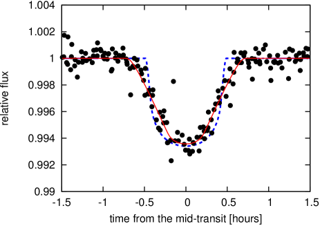
Figure 6.— Phase-folded K2 light curve (black points) around the transit of K2-28b. The best-fit transit model, integrated over the cadence of K2 observation ($\sim 29.4$ minutes), is shown by the red solid line. The transit model before the time-integration is shown by the blue dashed line.

Table 3Final Planetary Parameters

Parameter	Value
$P$ (days)	$2.260455\pm 0.000041$
$T_{c,0}$ (BJD)	$2456977.99012_{-0.00074}^{+0.00075}$
$R_{p}$ ($R_{\oplus}$)	$2.32\pm 0.24$
$i_{o}$ (∘)	$88.9_{-1.2}^{+0.8}$
$a$ (AU)	$0.0214\pm 0.0013$
$T_{\mathrm{eq}}$ (K) (Bond albedo: 0.0)	$568\pm 35$
$T_{\mathrm{eq}}$ (K) (Bond albedo: 0.4)	$500\pm 31$

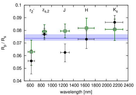
Figure 7.— Planet-to-star radius ratio ($R_{p}/R_{s}$) in each observed band (filled circles). The blue area represents $\pm 1\sigma$ of $R_{p}/R_{s}$ in the Kepler band. The horizontal errorbar for each band corresponds to the range of wavelength covered by the band. Note that the Kepler band covers the optical region between $437-835$ nm. The open squares are the measured $R_{p}/R_{s}$ for the cases that airmass cutoffs ($<2.2$) are applied (the $r_{2}^{\prime}$ and $z_{s,2}$ bands) and light curves are extracted with time-variable apertures (the $J$, $H$, and $K_{s}$ bands) in the fit.

Figure 6 shows the phase-folded K2 data (black points) along with our best-fit model (red solid line), and Table 3 summarizes our final result for the system parameters. Comparing the radius ratio by K2 data analysis with those by ground-based observations, $R_{p}/R_{s}$ from the optical to the infrared is consistent within $\sim 2\sigma$ (Figure 7: filled circles). The good agreement between the K2 transit depth and that in the $z_{\mathrm{s,2}}$ band, in which the best photometric precision was achieved from the ground, suggests that the transit-like signal is not caused by a background/bound eclipsing binary. Nonetheless, the transit depths in the $r_{2}^{\prime}$- and $K_{\mathrm{s}}$-bands exhibit a moderate disagreement. We will revisit this issue in Section 5.

The relatively short transit duration of K2-28b, in spite of the moderate impact parameter, suggests that the stellar radius is small and thus the star has a higher density. Indeed, using $a/R_{s}=17.9_{-2.8}^{+1.2}$ and Kepler’s third law, we estimate the stellar density as $\rho_{\star}/\rho_{\odot}=15.1_{-5.9}^{+3.2}$ solely from the transit light curve. Comparing this value with the spectroscopic estimate (Table 1), we find that they are compatible with each other, making it highly likely that K2-28b is transiting a cool star.

4. Validation of the Candidate

4.1. Resolved Sources in the Field

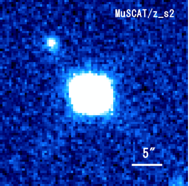
Figure 8.— MuSCAT’s on-focus image for K2-28 in the $z_{\mathrm{s,2}}$ band. North is up and east is left. Linear scaling is applied in this image.

As we noted, the SDSS image taken in 2000 suggests that K2-28 has a faint companion to its north-east at a separation of $\sim 5\farcs 2$, which could become a source of false positive. Figure 8 plots our latest $z_{\mathrm{s,2}}$-band image taken by MuSCAT on 2015 August 23 UT, in which we found the faint companion with the same magnitude difference as in SDSS, located further from K2-28. Considering the proper motion of K2-28 ($\mu_{\alpha}=-256\pm 3$ mas yr^-1 and $\mu_{\delta}=-195\pm 3$ mas yr^-1) (Ahn et al., 2012), the expected current separation between the two is $\sim 10^{\prime\prime}$ on the assumption that the fainter object is a background one. After calibrating the coordinates of both stars, we find that the faint companion stays at the almost same location while the current coordinate of K2-28 has slightly moved to $\mathrm{RA}=22:22:29.59,~{}\mathrm{Dec}=-07:57:22.78$. The current separation between the two is estimated as $10\farcs 36\pm 0\farcs 17$, which is fully consistent with the background scenario of the faint object.

Although the coordinate of the background star is outside of our custom-made aperture in the K2 photometry, a portion of its pixel response function (PRF) is involved in the aperture, meaning that the background star could still be a source of false positive. We checked the magnitude of its contamination on K2-28 assuming the averaged PRF for Kepler prime mission (Equation (10) in Coughlin et al., 2014). To estimate the fraction of the companion’s PRF that falls on our custom-made aperture, we simplified the aperture so that it is a circle encompassing all the aperture pixels with its radius being $8\farcs 44$. The resulting companion’s PRF fraction was estimated as $\sim 0.248$, and combining this with the magnitude difference between the two stars ($\Delta m_{\mathrm{kep}}\approx 4.82$), we estimated the maximum contamination from this companion as $\approx 3.0\times 10^{-3}$. The PRF for K2 could be larger than for the Kepler prime mission, but since the aperture does not extend to the coordinate of the background star, the PRF fraction cannot exceed $\sim 0.5$. Along with the fact that the maximum flux contamination from the companion star is smaller than the observed transit depth ($0.006-0.007$), we conclude that it is not responsible for the transit-like signal detected in our pipeline. Note that we also checked the current coordinate of K2-28 in the SDSS image, finding no bright object which could become a possible source of false positives.

4.2. Bayesian Statistical Calculation

We performed a Bayesian calculation of the false positive probability (FPP) that the signal arises from a background star (i.e., an eclipsing binary, EB) in the vicinity of the location of K2-28. The calculation does not address the probability that such a star is actually a binary on an eclipsing orbit, but address the probability that an appropriate star is close on the sky to produce the signal, and thus it is an upper limit on FPP. The procedure is described in detail in Gaidos et al. submitted, ApJ, and only briefly described here. The calculation multiplies a prior probability based on a model of the background stellar population by likelihoods from observational constraints. The synthetic background population at the location of K2-28 was constructed using TRILEGAL Version 1.6 (Vanhollebeke et al., 2009): to improve counting statistics, the population equivalent to 10 sq. deg. was computed. The background was computed to $m_{\mathrm{kep}}=23$, i.e. far fainter than the faintest object ($m_{\mathrm{kep}}\approx 19.5$) that could produce the signal if it were an EB with the maximum eclipse depth of 50%. The likelihood factors are the probabilities that (a) the background star can produce the observed transit depth; (b) the mean density of the background star is consistent with the observed transit duration; and (c) the background star does not appear in our Subaru ICRS-AO $K^{\prime}$-band imaging of the K2-28 (Section 2.5).

The calculation was performed by Monte Carlo: it sampled the synthetic background population randomly and placed them randomly and uniformly over a $15^{\prime\prime}$-radius circle centered on K2-28. Stars that violated the AO contrast ratio constraint (condition c) were excluded. Given the known orbital period and mean density of the synthetic star, the probability that a binary would have an orbit capable of producing the observed transit duration (condition b) was calculated assuming a Rayleigh distribution of orbital eccentricities with mean of 0.1. (Binaries on short-period orbits should quickly circularize.) To determine whether a background star could produce the observed transit signal with an eclipse depth $<50\%$ (condition a), we determined the relative contribution to the flux of K2-28 using bilinear interpolations of the PRF for detector channel 48 with the tables provided in the Supplement to the Kepler Instrument Handbook (E. Van Cleve & D. A. Caldwell, KSCI-19033). The calculations were performed in a series of 1000 Monte Carlo iterations and a running average used to monitor convergence. We found a FPP of $\approx 2\times 10^{-5}$ and therefore, we rule out the false positives by a background eclipsing binary.

4.3. Constraint on Possible Dilution Sources

The remaining false positive case is that a physically associated stellar companion is present around K2-28. The bound companion could have a transiting object (case A), or K2-28 could have a transiting object but its depth is diluted by the bound companion (case B). Our AO image achieves a $5\sigma$ contrast of $\sim 0.24$ at a separation of $0\farcs 1$, which translates to $\sim 5$ AU from K2-28. Thus, it is possible that a bound companion later than M4 dwarf is present within this distance from the central star. However, the similar values for the transit depth ($R_{p}/R_{s}$) from the optical to near infrared suggest that case A is unlikely, when the bound companion has a different spectral type from K2-28.

To quantify this statement, we refit the observed light curves introducing a “dilution factor” $D$, defined as the ratio of the companion’s flux to that of K2-28 in each bandpass. The companion has to be equal to or later than M4 dwarf since our spectroscopy implies K2-28 is the dominant source of brightness in the system. Thus, $D$ is in general larger in the infrared than in the optical. On the assumption that the later-type companion has a transiting object (case A), we search for a solution to the observed light curves as in Section 3. We assume various stellar types for the companion, and employ the contrast ratio for each band from Kraus & Hillenbrand (2007). We simply use the $r$ and $z$ magnitudes in Kraus & Hillenbrand (2007) to represent the MuSCAT $r^{\prime}_{2}$ and $z_{\mathrm{s,2}}$ bands, and $m_{\mathrm{kep}}$ is computed by $0.1m_{g}+0.9m_{r}$. As a result of the global fit to the ground-based transit follow-ups along with the K2 light curve including $D$, we find that a companion later than M4 dwarf leads to an incompatible result: in case of an M5 dwarf companion, the intrinsic radius ratio of the eclipsing objects in the optical (e.g., $R_{p}/R_{s}=0.206\pm 0.003$ for the Kepler band) becomes inconsistent with that in the infrared (e.g., $R_{p}/R_{s}=0.134\pm 0.008$ for the $J$ band) with $>5\sigma$. Hence, the putative bound companion (having a transiting object) around K2-28, if any, has to be another M4 dwarf. Even in this case, the transiting object falls on the planetary regime considering that the maximum possible dilution (M4+M4 binary case) brings about an underestimation of the radius ratio by a factor of $\sim\sqrt{2}$.

For the rest of the discussion, we resort to the statistics to constrain the possible dilution scenario by computing the probability that “K2-28 has an almost identical bound stellar companion”. First, the probability that an M dwarf ($0.1-0.5M_{\odot}$) has any stellar companion is $26\pm 3~{}\%$, and the probability that their mass ratio $q$ is greater than 0.75 ($\approx$ mass ratio between M4 and M5 dwarfs) is $0.57_{-0.27}^{+0.17}$ on the assumption that the probability distribution of $q$ follows $\propto q^{\gamma}$ with $\gamma=1.9\pm 1.7$ (Duchêne & Kraus, 2013). Then, adopting the log-normal distribution for the period $P$, we estimate the probability that binary’s semi-major axis is smaller than 5 AU as $\approx 0.49$ (Duchêne & Kraus, 2013). Thus, the total probability that K2-28 has such an M4 companion is $\approx 0.0721_{-0.036}^{+0.023}$. This is not critically low, yet we can safely say that it is more likely that K2-28 is a single star with a transiting super-Earth/mini-Neptune.

We note that case B of the dilution scenario is also possible, but this possibility is not so high as well following the same discussion above. In order to estimate the maximum radius ratio, we repeat the fit of the light curves with $D=1.0$, representing the case that a bound M4 dwarf identical to K2-28 is present in the system. The global fit to the observed light curves yields $R_{p}/R_{s}=0.104_{-0.002}^{+0.004}$, corresponding to $R_{p}\approx 3.27R_{\oplus}$. Again, this is an upper limit of the planet radius, and the planetary size is much closer to $R_{p}\approx 2.32R_{\oplus}$ when the dilution source is later than M4. All these dilution possibilities could be settled by taking a high resolution spectrum of the target and checking the binarity from the line blending, although the faintness of the target would make it challenging in the optical region ($m_{V}\approx 16.1$).

5. Discussion and Summary

We have conducted intensive follow-up observations for K2-28, which emerged as a planet-host candidate within the ESPRINT collaboration. Our optical spectroscopy indicates that K2-28 is a metal-rich M4 dwarf, located at $53\pm 8$ pc away from us. Based on the absence of bright sources in the AO image taken by Subaru/IRCS, we computed the probability that the transit-like signal is caused by a background eclipsing binary, and showed that such an FPP is very low ($\approx 2\times 10^{-5}$). The remaining possible false positive scenario is that a physically associated companion has a transiting object, but this still puts K2-28b in the planetary regime considering the maximum possible dilution case. Our ground-based transit follow-ups using OAO/MuSCAT and IRSF/SIRIUS revealed similar transit depths in different bands from the optical to the near infrared, thus showing such a bound companion is not likely to exist around K2-28, with the probability being $\approx 0.0721_{-0.036}^{+0.023}$.

It should be emphasized that the high cadence photometry of ground-based follow-ups helped to break the degeneracy between the system parameters. The poor sampling of the K2 data makes the transit curve V-shaped as shown in Figure 6, which could be explained by a grazing eclipsing binary, but follow-up transits exhibit flat bottoms in all bands, which are suggestive of a small transiting body. Even in the absence of a prior probability on the stellar density in fitting the follow-up transits, we could obtain a relatively tight constraint on the scaled semi-major axis and radius ratio. This case clearly demonstrates the importance of transit follow-ups from the ground to validate planetary candidates with relatively short transit durations.

Despite the careful analysis for the follow-up transits using GP, the transit depths in the $r_{2}^{\prime}$ and $K_{\mathrm{s}}$ bands shows a moderate disagreement ($\sim 2\sigma$) with that in the Kepler band as shown in Figure 7. As discussed below, these differences in $R_{p}/R_{s}$ are significantly larger than the ones expected from the different optically-thick planet radii in individual bands ($\Delta(R_{p}/R_{s})\approx 0.003$ at the most assuming a hydrogen-rich atmosphere). The disagreement in the $r_{2}^{\prime}$ band could be due to the lack of egress combined with the small number of data points during the transit. At the end of the OAO/MuSCAT run, the target was also low in elevation, suggesting that higher airmass may have caused some systematics. To take account of the airmass-related systematics, we also performed a global fit to the observed light curves including an airmass-dependent GP term in Equation (5). The result of the fit was fully consistent with the result without the airmass-dependent GP term (i.e., $R_{p}/R_{s}=0.057_{-0.010}^{+0.009}$ for the $r_{2}^{\prime}$ band). On the other hand, if we simply remove the flux data taken at higher airmass ($>2.2$) from the OAO dataset, the global fit yields $R_{p}/R_{s}=0.063_{-0.011}^{+0.009}$ for the $r_{2}^{\prime}$ band, which agrees with $R_{p}/R_{s}$ in the Kepler band with $\sim 1\sigma$. This treatment is rather arbitrary so that we do not claim its result as the final one. Further transit observations covering a whole transit would be able to settle this issue.

We also investigated the reason for the disagreement in the $K_{\mathrm{s}}$ band by checking the raw images taken by IRSF. We found that the FWHM of the target image slightly changed (by $\sim 20\%$) during our IRSF observation, and that variation was not a monotonic function of time; the FWHM takes its maximum during the transit. Although we have incorporated the FWHM as an input auxiliary variable in the GP regression to the correlated noises, this significant variation in FWHM may have caused further systematics in the extracted light curves.

To further investigate this possibility, we adopt time-variable apertures and set each aperture radius as FWHM multiplied by a constant value (e.g., 0.6), and extracted light curves again. Then, following the fitting procedure described in Section 3, we estimate the planet-to-star radius ratio for each band. Consequently, we find $R_{p}/R_{s}=0.081_{-0.009}^{+0.008}$ for the $K_{\mathrm{s}}$ bands (Figure 7: open squares). This value is consistent with the transit depth in the Kepler band ($R_{p}/R_{s}=0.074_{-0.002}^{+0.003}$), but the photometric precision turns out to be much worse than the fixed-aperture photometry. The reason for this discrepancy between the light curves for fixed and time-variable apertures is not known, but imperfect correction for flat-fielding or inclusion of scattered light from a neighboring star could be relevant.

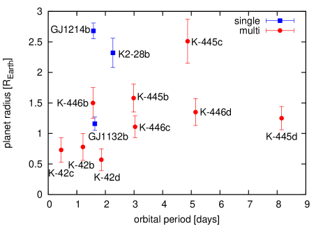
Figure 9.— Transiting planets around M dwarfs cooler than $T_{\mathrm{eff}}\leq 3400$ K. Planets in single and multiple systems are shown in blue squares and red circles, respectively (Charbonneau et al., 2009; Muirhead et al., 2012, 2015; Berta-Thompson et al., 2015). “Kepler-” is abbreviated as “K-” in this plot.

Dressing & Charbonneau (2013) found that while the occurrence rate of Earth-sized planets ($R_{p}<1.4R_{\oplus}$) around coolest M dwarfs monitored by Kepler is consistent with that around hotter M dwarfs ($T_{\mathrm{eff}}\geq 3723$ K), the occurrence rate of super-Earths around cooler M dwarfs is significantly smaller than that around hotter M dwarfs. Figure 9 plots the transiting planets around M dwarfs later than M3. Among those planets, the transiting planets with $R_{p}\geq 2.0R_{\oplus}$ are only GJ 1214b, Kepler-445c, and K2-28b. We note that their hosts are all metal-rich stars, which is in marked contrast to the metal poor hosts, Kepler-42, Kepler-446, and GJ 1132, having only Earth-sized (or sub-Earth-sized) planets. The occurrence rate calculated by Dressing & Charbonneau (2013) could contain $T_{\mathrm{eff}}$-dependent systematic errors in the stellar (and thus planet) radii, arising from the adopted models which become unreliable for lower $T_{\mathrm{eff}}$. With more samples as presented here, one can discuss the statistical property of planets around cooler M dwarfs more accurately.

With the relatively bright host star in the near infrared and moderate transit depth, K2-28 is a good target for future follow-up studies. It is particularly tempting to compare K2-28b with another well-studied super-Earth/mini-Neptune, GJ 1214b, in terms of atmospheric characteriztions. Using the semi-major axis of $a=0.0214\pm 0.0013$ AU and K2-28’s radius and effective temperature in Table 1, we find that K2-28b happens to receive almost an equivalent insolation from its host star as GJ 1214b (incident energy fluxes $S_{\mathrm{inc}}\approx 17.3S_{\oplus}$ for K2-28b and $S_{\mathrm{inc}}\approx 17.6S_{\oplus}$ for GJ 1214b, respectively). Kreidberg et al. (2014) conducted a spectro-photometry with the Wide Field Camera 3 (WFC3) on the Hubble Space Telescope (HST), and as a result of analyzing 12 transits of GJ 1214b, they achieved a precision of $30-40$ ppm for the transit depth in the individual spectroscopic channel between $1.15-1.65\mu$m. Since the transit depth variation against wavelength scales as $\Delta(R_{p}^{2}/R_{s}^{2})\propto 2(R_{p}/R_{s})^{2}(H/R_{p})$, where $H$ is the scale height, this variation for K2-28 as a function of wavelength would be $0.30\times$ that for GJ 1214b. If one conducts a similar observation for K2-28 to the one conducted by Kreidberg et al. (2014), observing the same number of transits with HST, we expect a precision of $70-80$ ppm for the transit depth measurement on the assumption that the uncertainty is dominated by the photon-limited shot noise ($\Delta m_{H}=1.94$ mag and transit duration of $\sim 60$ minutes). This level of precision is sufficient to confirm or rule out the atmospheres dominated by hydrogen or methane, for which the scale height equal to GJ 1214b would lead to $\Delta(R_{p}^{2}/R_{s}^{2})\sim 450$ ppm and $\sim 150$ ppm in variation amplitudes, respectively. Ruling out the water- or carbon-dioxide-dominated atmospheres ($\sim 80$ ppm and $\sim 20$ ppm, respectively) could be challenging, but increasing the number of observed transits will help.

Searching for additional planets in the system is also important to understand the architecture of planetary systems around mid-M dwarfs. Muirhead et al. (2015) showed that a significant fraction ($21_{-5}^{+7}~{}\%$) of mid-M dwarfs hosts multiple planets within 10 days. Concerning K2-28, we could not find evidence of another transiting planet in our BLS analysis. The sparse sampling of the K2 data during the transit makes it complicated to search for possible transit timing variations (TTVs), but further intensive ground-based transit follow-ups would find or at least be able to put a constraint on the presence of additional bodies. While K2-28 is faint in the optical, it is relatively bright in the NIR ($m_{H}=11.03\pm 0.02$ mag), and thus is likely within the reach of existing and planned NIR radial velocity instruments (e.g., IRD, CARMENES, SPIrou, HPF; Kotani et al., 2014; Quirrenbach et al., 2014; Artigau et al., 2014; Mahadevan et al., 2014), which could also reveal any non-transiting planets.

References

- Ahn et al. (2012) Ahn, C. P., et al. 2012, ApJS, 203, 21
- Aldering et al. (2002) Aldering, G., et al. 2002, in Society of Photo-Optical Instrumentation Engineers (SPIE) Conference Series, Vol. 4836, Survey and Other Telescope Technologies and Discoveries, ed. J. A. Tyson & S. Wolff, 61–72
- Allard et al. (2013) Allard, F., Homeier, D., Freytag, B., Schaffenberger, , W., & Rajpurohit, A. S. 2013, Memorie della Societa Astronomica Italiana Supplementi, 24, 128
- Armstrong et al. (2015) Armstrong, D. J., et al. 2015, A&A, 582, A33
- Artigau et al. (2014) Artigau, É., et al. 2014, in Society of Photo-Optical Instrumentation Engineers (SPIE) Conference Series, Vol. 9147, Society of Photo-Optical Instrumentation Engineers (SPIE) Conference Series, 914715
- Bean et al. (2010) Bean, J. L., Miller-Ricci Kempton, E., & Homeier, D. 2010, Nature, 468, 669
- Berta-Thompson et al. (2015) Berta-Thompson, Z. K., et al. 2015, Nature, 527, 204
- Boyajian et al. (2012) Boyajian, T. S., et al. 2012, ApJ, 757, 112
- Charbonneau et al. (2009) Charbonneau, D., et al. 2009, Nature, 462, 891
- Claret et al. (2013) Claret, A., Hauschildt, P. H., & Witte, S. 2013, A&A, 552, A16
- Coughlin et al. (2014) Coughlin, J. L., et al. 2014, AJ, 147, 119
- Crossfield et al. (2015) Crossfield, I. J. M., et al. 2015, ApJ, 804, 10
- Cushing et al. (2004) Cushing, M. C., Vacca, W. D., & Rayner, J. T. 2004, PASP, 116, 362