Herschel-Planck dust optical depth and column density maps

We present optical depth and temperature maps of the Perseus molecular cloud, obtained combining dust emission data from the Herschel and Planck satellites and 2MASS/NIR dust extinction maps. The maps have a resolution of 36 arcsec in the Herschel regions, and of 5 arcmin elsewhere. The dynamic range of the optical depth map ranges from $1\times 10^{-2}\,\mathrm{mag}$ up to $20\,\mathrm{mag}$ in the equivalent K band extinction. We also evaluate the ratio between the $2.2\text{\,}\mathrm{\SIUnitSymbolMicro m}$ extinction coefficient and the $850\text{\,}\mathrm{\SIUnitSymbolMicro m}$ opacity. The value we obtain is close to the one found in the Orion B molecular cloud. We show that the cumulative and the differential area function of the data (which is proportional to the probability distribution function of the cloud column density) follow power laws with index respectively $\simeq-2$, and $\simeq-3$. We use WISE data to improve current YSO catalogs based mostly on Spitzer data and we build an up-to-date selection of Class I/0 objects. Using this selection, we evaluate the local Schmidt law, $\Sigma_{\mathrm{YSO}}\propto\Sigma_{\mathrm{gas}}^{\beta}$, showing that $\beta=2.4\pm 0.6$. Finally, we show that the area-extinction relation is important for determining the star formation rate in the cloud, which is in agreement with other recent works.

1 Introduction

Understanding the physical processes that rule star formation is fundamental to improve our knowledge of galaxy formation and evolution across cosmic time.

An essential step towards reaching a better comprehension of star formation inside our Galaxy is to establish the relationship between the star formation rate (SFR) and the physical properties of the interstellar gas. Schmidt (1959) conjectured that ”the SFR depends on the gas density and […] varies with a power law of the gas density.” Schmidt argued that the index of the power law in the solar neighborhood was $\sim 2$. Kennicutt (1998) expressed the law as $\Sigma_{\mathrm{SFR}}=\kappa\Sigma_{\mathrm{gas}}^{\beta}$, where $\Sigma_{\mathrm{gas}}$ and $\Sigma_{\mathrm{SFR}}$ are the surface densities of the gas and of star formation rate. Kennicutt tested the Schmidt law in a heterogeneous sample of star forming galaxies and showed that a power law scaling relation exists between them and is characterized by an index $\beta=1.6$. Using observations of local disc and starburst galaxies, Bigiel et al. (2008) found a complex scaling between $\Sigma_{\mathrm{SFR}}$ and $\Sigma_{\mathrm{gas}}$, which could not be described by a single power law. On smaller, sub-kpc scales, Lada et al. (2013) showed that there is no Schmidt scaling relation between local giant molecular clouds, but a series of observational studies demonstrated that a Schmidt scaling law exists within some local molecular clouds (Heiderman et al., 2010; Gutermuth et al., 2011; Lombardi et al., 2013; Lada et al., 2013; Evans et al., 2014; Harvey et al., 2014).

In order to be able to understand the detailed interplay between the structure of molecular clouds and their local star formation rates (as opposed to the global one often considered), we are carrying out a coordinated study of molecular clouds in the Gould belt. We use a combination of Planck and Herschel dust emission data, calibrated using near infrared (NIR) dust extinction. This technique guarantees an optimal resolution of the cloud column density maps (corresponding to the Herschel/SPIRE500 $36\text{\,}\mathrm{a}\mathrm{r}\mathrm{c}\mathrm{s}\mathrm{e}\mathrm{c}$ resolution), better than the one of standard NIR extinction maps in the region of the sky we are considering. In our first paper we considered the Orion giant molecular cloud (Lombardi et al., 2014); here we focus on Perseus.

The Perseus cloud was first observed by Barnard, who cataloged a portion of it as Barnard 1-5 and Barnard 202-206. Since then, the cloud was extensively studied using molecular line emission (Ridge et al., 2006), star count extinction (Bachiller & Cernicharo, 1984), and dust continuum emission (Hatchell et al., 2005; Kirk et al., 2006; Enoch et al., 2006). Distance estimates for Perseus vary (Herbig & Jones, 1983; Cernis, 1990, 1993; Bally et al., 2008; Hirota et al., 2008; Schlafly et al., 2014); we use $240\text{\,}\mathrm{p}\mathrm{c}$ for consistency with Lombardi et al. (2010). Perseus is the prototype intermediate mass star forming region, with young B stars and two clusters, IC 348 (Muench et al., 2007) and NGC1333 (Lada et al., 1996). The complex seems to be associated with the Perseus OB2 association (de Zeeuw et al., 1999). Recently, Herschel observations were used to characterize small regions of the cloud. Pezzuto et al. (2012) studied two star forming dust condensations, B1-bS and B1-bN in the B1 region (see Fig. 1). They conclude that these two sources could be good examples of the first hydrostatic core phase. Sadavoy et al. (2012) presented observations of the B1-E region and proposed that it may be forming the first generation of dense cores. Finally, Sadavoy et al. (2014) identified and characterized 28 candidate Class 0 protostars in the whole cloud, four of which are newly discovered. They also found that the star formation efficiency of the clumps, as traced by Class 0 protostars, correlates strongly with the flatness of their respective column density distribution at high values. A global study of the Perseus cloud properties with Herschel data is still missing, and constitutes the main goal of this paper.

This paper is organized as follows. In Section 2 we present the data used in this work; in Section 3 we briefly describe the data reduction process; in Section 4 we apply the method to study the Perseus molecular cloud and present the column density and temperature maps ; in Section 5 we derive the local Schmidt law; finally, in Section 6 we present a summary.

2 Data

Perseus was observed as part of the Gould Belt Survey (André et al., 2010), one of the Herschel satellite key projects. The cloud was observed using the two photometers PACS (Poglitsch et al., 2010) and SPIRE (Griffin et al., 2010), in five bands, centered approximately at $70\text{\,}\mathrm{\SIUnitSymbolMicro m}160\text{\,}\mathrm{\SIUnitSymbolMicro m}250\text{\,}\mathrm{\SIUnitSymbolMicro m}350\text{\,}\mathrm{\SIUnitSymbolMicro m}500\text{\,}\mathrm{\SIUnitSymbolMicro m}$. Table 1 gives an overview of the observation used in this work. Dust maps derived by the Planck Collaboration (Planck Collaboration et al., 2014), and the near infrared extinction maps produced by Lombardi et al. (2010) through the NICEST method (Lombardi, 2009) are also used. We selected the region (corresponding to the Perseus molecular cloud) with galactic coordinates:

$$155^{\circ}<l<165^{\circ},\hskip 14.22636pt-25^{\circ}<b<-15^{\circ}.$$ (1)

Additionally, we employed the AllWISE data release (Wright et al., 2010; Mainzer et al., 2011) to select Young Stellar Objects (YSOs) from their colors. The WISE satellite observed the whole sky in four infrared bands, often referred to as W1, W2, W3, and W4, with wavelengths centered at $3.4\text{\,}\mathrm{\SIUnitSymbolMicro m}4.6\text{\,}\mathrm{\SIUnitSymbolMicro m}12\text{\,}\mathrm{\SIUnitSymbolMicro m}22\text{\,}\mathrm{\SIUnitSymbolMicro m}$. We retrieved 1.43 million sources from the WISE point source catalog in the science field and 1.63 million sources in the control field. We rejected any source with contamination and confusion flags and we further restricted the selection to those measurements with errors $\sigma<0.15\,\mathrm{mag}$ in all the WISE bands. The AllWISE source catalog contains associations with the 2MASS Point Source Catalog (Skrutskie et al., 2006). The precision adopted by the AllWISE collaboration for the 2MASS association is 3”. In addition, we required photometric errors in the 2MASS bands to be smaller than $0.1\,\mathrm{mag}$ .

Table 1: Herschel parallel mode observation used.

Target Name	Obs. ID	RA	DEC	Wavelengths ($\mu m$)	Obs. date	Exp. Time (s)
Perseus S	1342190326	3h 29m 38s	+30 54’ 33”	SPIRE, PACS 70 and 160	2010-09-02	14765
Perseus N	1342214504	3h 42m 51s	+32 01’ 38”	SPIRE, PACS 70 and 160	2011-19-2	11624

3 Method

The reduction technique is very close to the one presented by Lombardi et al. (2014) and therefore we only briefly summarize it in this section.

3.1 Dust Model

Dust is optically thin at the Herschel observation frequencies (at least for $\lambda>$ $160\text{\,}\mathrm{\SIUnitSymbolMicro m}$), and therefore its emission can be modeled as a modified black body:

$$I_{\nu}=B_{\nu}\left(T\right)\left(1-e^{-\tau_{\nu}}\right)\simeq B_{\nu}\left(T\right)\tau_{\nu}.$$ (2)

Here $B_{\nu}\left(T\right)$ is the black body function at the temperature $T$ and the optical thickness $\tau_{\nu}$ is taken to be a power law of the frequency $\nu$:

$$\tau_{\nu}=\tau_{\nu_{0}}\left(\frac{\nu}{\nu_{0}}\right)^{\beta}.$$ (3)

The frequency $\nu_{0}$ is an arbitrary reference frequency that we set as $\nu_{0}=353\,\mathrm{GHz}$ (corresponding to $\lambda=$850\text{\,}\mathrm{\SIUnitSymbolMicro m}$$), similarly to what was done by the Planck collaboration (Planck Collaboration et al., 2014).

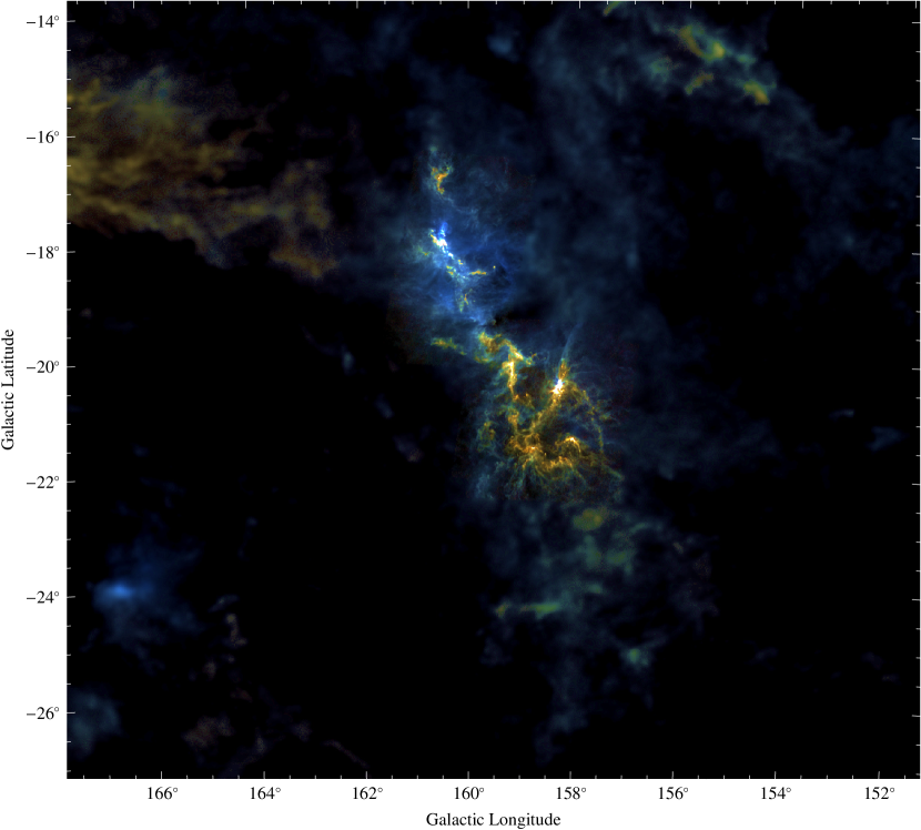
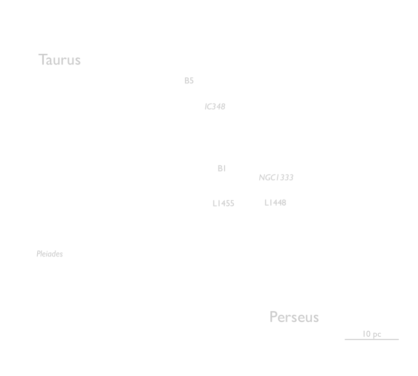
Figure 1: Composite three-colors image showing Herschel/SPIRE intensities for the region considered, where available (with the $250\text{\,}\mathrm{\SIUnitSymbolMicro m}350\text{\,}\mathrm{\SIUnitSymbolMicro m}500\text{\,}\mathrm{\SIUnitSymbolMicro m}$ bands shown in blue, green, and red). For regions outside the Herschel coverage, we used the Planck/IRAS dust model ($\tau_{\mathrm{850}}$, T, $\mathrm{\beta}$) to predict the intensity that would be observed at the SPIRE passbands. user /Subtype /Link /Border [0 0 0]/A ¡¡ /S/JavaScript /JS ( var aOCGs = this.getOCGs(), Layer; var Layers = ”fig:2b,fig:2a”.split(”,”), Active = -1, i, l; for (l=0; l¡Layers.length; l++) Layer = Layers[l]; for (i=0; aOCGs & i¡aOCGs.length; i++) if (aOCGs[i].state aOCGs[i].name == Layer) Active = l; aOCGs[i].state = false; if (Active ¿= 0) break; if (Active == -1) for (l=0; l¡Layers.length; l++) if (Layers[l] == ) Active = l; Active = Active + 1; if (Active == Layers.length) Active = 0; Layer = Layers[Active]; for (i=0; aOCGs & i¡aOCGs.length; i++) if (aOCGs[i].name == Layer) aOCGs[i].state = true; ) ¿¿ Toggle labels

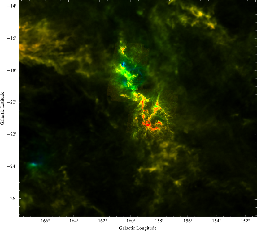
Figure 2: Combined optical depth-temperature map for Perseus. The image shows the optical depth as intensity and the temperature as hue, with red (blue) corresponding to low (high) temperatures.

3.2 SED fitting

The aim of our work is to infer the effective dust color temperature and the optical depth from the fluxes measured by Herschel at $250\text{\,}\mathrm{\SIUnitSymbolMicro m}350\text{\,}\mathrm{\SIUnitSymbolMicro m}500\text{\,}\mathrm{\SIUnitSymbolMicro m}$, following Lombardi et al. (2014), and also PACS $160\text{\,}\mathrm{\SIUnitSymbolMicro m}$ where available. For this purpose, we first convolved all the Herschel data to the beam size of SPIRE $500\text{\,}\mathrm{\SIUnitSymbolMicro m}$, i.e. to $36\,\mathrm{arsec}$ and then we fitted the observed spectral energy distribution with the function (2), that was integrated over the Herschel bandpasses. The detailed fitting procedure is described in detail in Lombardi et al. (2014), however we report here a brief outline of the basic steps used to generate the maps:

• For each SPIRE band we multiply for the correcting factor $C=K_{4e}/K_{4p}$. Since the extended source calibration method changed as a consequence of the work by Griffin et al. (2013), the correcting factors are not the same as those used in Lombardi et al. (2014). Specifically, $C$ is now equal to $(0.9986,1.0015,0.9993)$, while before it was $C=(0.9828,0.9834,0.9710)$ for the $250\text{\,}\mathrm{\SIUnitSymbolMicro m}350\text{\,}\mathrm{\SIUnitSymbolMicro m}500\text{\,}\mathrm{\SIUnitSymbolMicro m}$ bands respectively. However, this change doesn’t have a significant impact on the final maps.

• We perform an absolute flux calibration for the Herschel bands, using Planck maps.

• We assume a modified black body SED and we compute the expected flux at each reference passband.

• We modify the SED until we obtain a good match between the observed and theoretical fluxes. For this step we use a simple $\chi^{2}$ minimization technique that takes into account the calibration errors.

For the analysis presented here, we used the HIPE (Ott, 2010) extended emission level 2.5 products for SPIRE data and Unimaps for PACS data. For PACS data it is possible to use Scanamorphos, however there is no significant difference between the two maps.

Figure 1 shows a color-composite image of the combined reduced Herschel/SPIRE data for the region considered here, together with the predicted fluxes from Planck at the three SPIRE passbands for locations outside the Herschel coverage.

3.3 Optical depth and temperature maps

Figure 2 shows the combined optical depth-temperature map: the effective dust temperature is represented using different values of hue, while the intensity is proportional to the optical depth. Figures 3 and 4 individually show the temperature and optical depth maps.

Note that Planck data have lower resolution (5 arcmin instead of 36 arcsec) and a significantly lower noise. In particular, the error on the regions covered by Planck data is much smaller than that on the Herschel areas. Figs. 3 and 4 highlight the differences in optical depth and temperature that characterize the cloud.

 

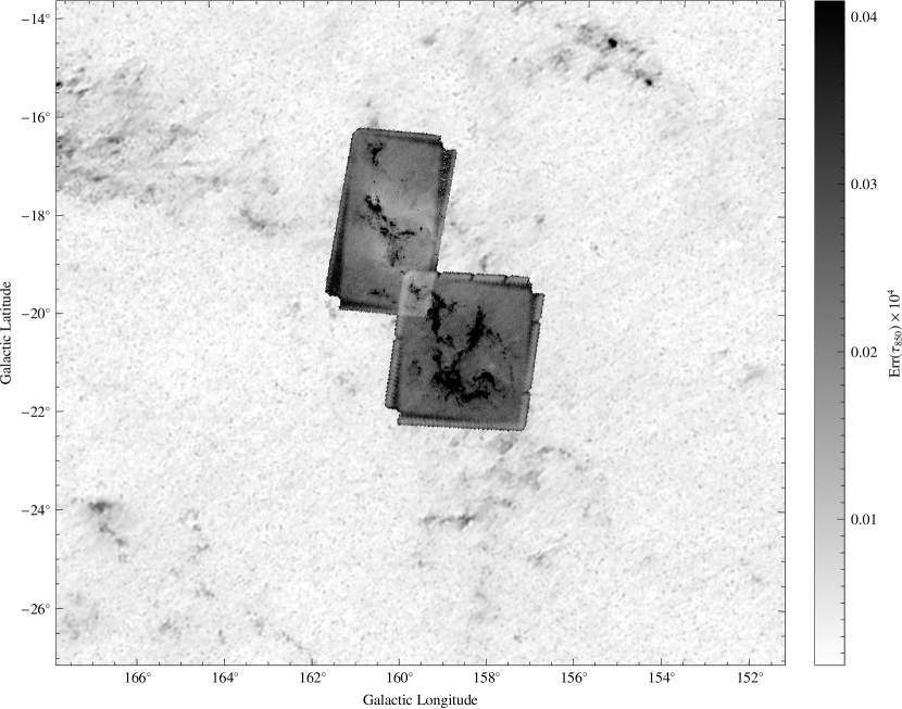
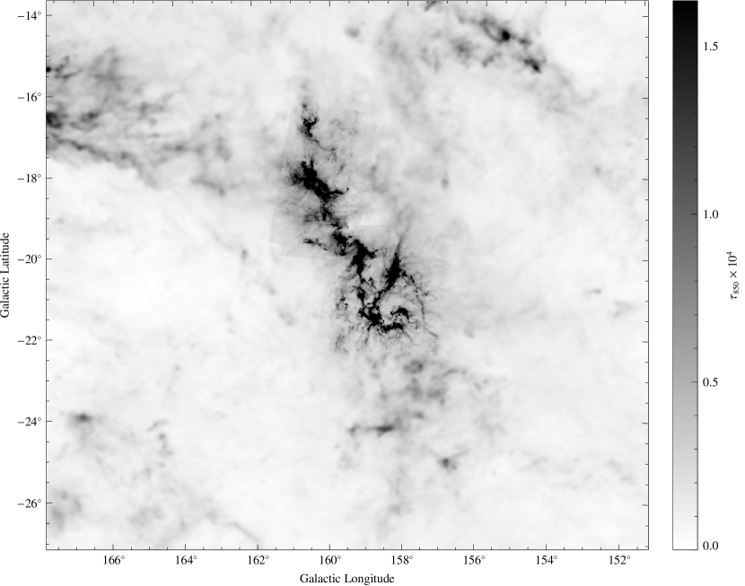
Figure 3: Optical depth map of the field and, on a user /Subtype /Link /Border [0 0 0]/A ¡¡ /S/JavaScript /JS ( var aOCGs = this.getOCGs(), Layer; var Layers = ”fig:3a,fig:3b”.split(”,”), Active = -1, i, l; for (l=0; l¡Layers.length; l++) Layer = Layers[l]; for (i=0; aOCGs & i¡aOCGs.length; i++) if (aOCGs[i].state aOCGs[i].name == Layer) Active = l; aOCGs[i].state = false; if (Active ¿= 0) break; if (Active == -1) for (l=0; l¡Layers.length; l++) if (Layers[l] == ) Active = l; Active = Active + 1; if (Active == Layers.length) Active = 0; Layer = Layers[Active]; for (i=0; aOCGs & i¡aOCGs.length; i++) if (aOCGs[i].name == Layer) aOCGs[i].state = true; ) ¿¿ different layer, the corresponding error map. This figure, as the following one (Fig. 3), is produced by the method described in the text, using the reduced fluxes of SPIRE and the expected fluxes at SPIRE frequencies deduced from the Planck maps (Planck Collaboration et al., 2014).

 

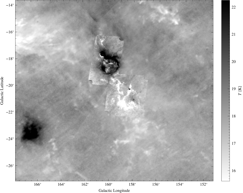
Figure 4: Temperature map of the field, and, on a user /Subtype /Link /Border [0 0 0]/A ¡¡ /S/JavaScript /JS ( var aOCGs = this.getOCGs(), Layer; var Layers = ”fig:4a,fig:4b”.split(”,”), Active = -1, i, l; for (l=0; l¡Layers.length; l++) Layer = Layers[l]; for (i=0; aOCGs & i¡aOCGs.length; i++) if (aOCGs[i].state aOCGs[i].name == Layer) Active = l; aOCGs[i].state = false; if (Active ¿= 0) break; if (Active == -1) for (l=0; l¡Layers.length; l++) if (Layers[l] == ) Active = l; Active = Active + 1; if (Active == Layers.length) Active = 0; Layer = Layers[Active]; for (i=0; aOCGs & i¡aOCGs.length; i++) if (aOCGs[i].name == Layer) aOCGs[i].state = true; ) ¿¿ different layer, the corresponding error map.

Referring to the temperature map (Fig. 4), we can note that the regions IC 348 and G159.6-18.5 present a higher temperature than the rest of the cloud and the ring of dust that surround the star HD 278942 (Andersson et al., 2000) is particularly visible. The temperature ranges between $\sim 10\,\mathrm{K}$ and $\sim 36\,\mathrm{K}$.

3.4 Extinction conversion

In order to compare the results obtained here with other observations, we converted the optical depth $\tau_{850}$ to the extinction $A_{K}$. For this purpose, we smoothed the optical depth map to the same resolution as the extinction map (2.5 arcmin) of the region (Lombardi et al., 2010). We assumed that within the range $0-2\times 10^{-4}$, the law that describes the relation between $\tau_{850}$ and $A_{\it{K}}$ is linear (see Fig. 5):

$$A_{\it{K}}=\gamma\tau_{850}+\delta.$$ (4)

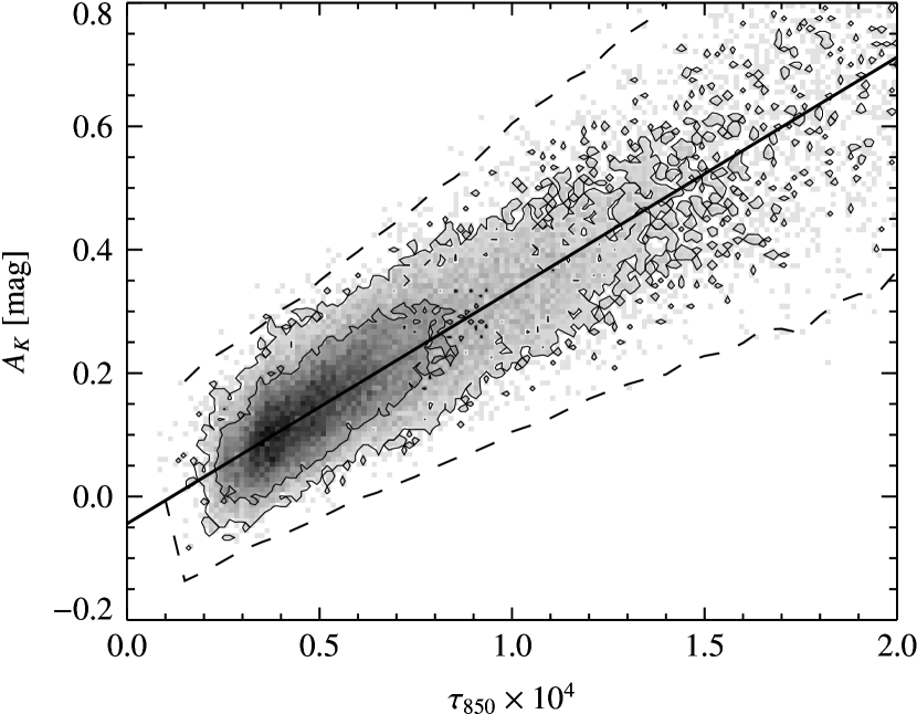
Figure 5: Relationship between submillimiter optical-depth and NIR extinction in Perseus. The image shows the best linear fit, used to calibrate the data (solid line), together with the expected $3\sigma$ region (dashed lines), as calculated from direct error propagation in the extinction map. The contours enclose respectively the 68% and the 95% of the points.

The slope $\gamma$ is proportional to the opacity $\kappa_{850}$ and to the extinction coefficient in the $K$ band, $C_{\mathrm{2.2}}$. Since the extinction in $K$ band is defined as:

$$A_{K}=-2.5\log_{10}\left(\frac{I_{\mathrm{obs}}}{I_{\mathrm{I_{true}}}}\right)=2.5(\log_{10}\mathrm{e})\,C_{2.2}\Sigma_{\mathrm{dust}},$$ (5)

the relationship between $\gamma$ and $C_{2.2}$ is simply $\gamma\leavevmode\nobreak\ \simeq\leavevmode\nobreak\ 1.0857\leavevmode\nobreak\ C_{2.2}\leavevmode\nobreak\ /\leavevmode\nobreak\ \kappa_{850}$. The coefficient $\delta$ is associated with uncertainties in the absolute flux calibration of Herschel, or to uncertainties in the extinction maps, or both. Through a $\chi^{2}$ minimization method, we obtained the following values for the two parameters:

$$\left\{\begin{aligned} \gamma&=3931\pm 274\,\mathrm{mag},\\ \delta&=-0.05\pm-0.02\times 10^{-6}\,\mathrm{mag}.\\ \end{aligned}\right.$$ (6)

The fact that $\delta$ is close to zero confirms the goodness of the calibration of Herschel data and of the extinction map. The value obtained for the slope $\gamma$ is quite close to the ones found by Lombardi et al. (2014) for Orion A and B ($\gamma_{\mathrm{Orion\,A}}=2640\,\mathrm{mag}$ and $\gamma_{\mathrm{Orion\,B}}=3460\,\mathrm{mag}$). Being proportional to the extinction coefficient $C_{2.2}$ and the opacity at $850\text{\,}\mathrm{\SIUnitSymbolMicro m}$, the coefficient $\gamma$ is related to the dust composition and grain distribution, and therefore differences in the values of $\gamma$ are likely related to differences in these quantities.

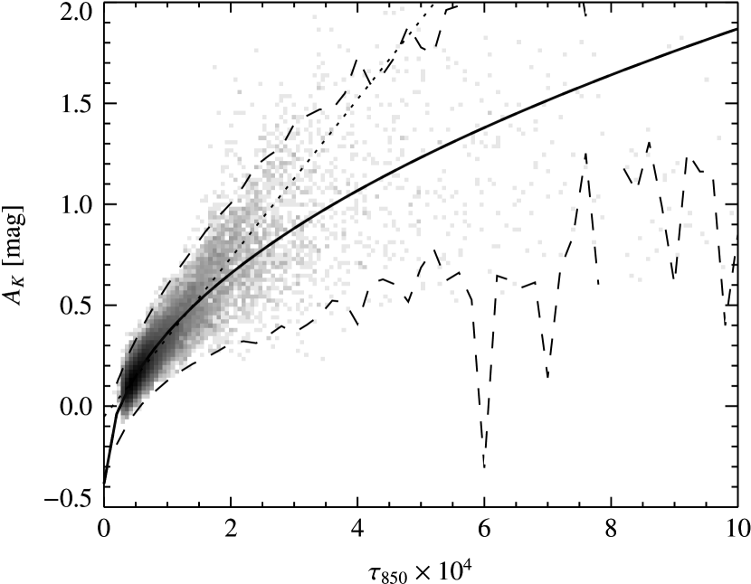
Figure 19: Relation between 353 GHz optical depth and the infrared NICEST extinction map, for $\tau_{850}\times 10^{4}\leq 10$. The relation deviates from the linearity for high extinction values, as shown by the fit (solid line).The dashed lines represent the expected $3\sigma$ region. We also report in this plot the linear fit shown in Fig. 5 (dotted line).

If we consider a wider range of values (see Fig. 19), with $\tau\times 10^{4}\leq 10$, the relation unexpectedly deviates from the linear law. In this case the law between $\tau_{850}$ and $A_{\it{K}}$ can be fitted by the empirical relation:

$$A_{\it{K}}=c_{1}+c_{2}\tau_{850}^{c_{3}}.$$ (7)

The best fit values for the three parameters are:

$$\left\{\begin{aligned} c_{1}&=-0.38447\pm 6.9\times 10^{-05}\,\mathrm{mag},\\ c_{2}&=61\pm 5\,\mathrm{mag},\\ c_{3}&=0.47973\pm 2.6\times 10^{-05}.\\ \end{aligned}\right.$$ (8)

The deviation from the linear regime might be due to either the inclusion of regions in the extinction map where a large number of embedded sources are present or the lack of background stars at highest extinction. In order to better understand the problem, we created a map (Fig. 6) that shows the difference between the extinction values evaluated from the extinction map and from the Herschel data using the linear scaling of Eq. (4). The highest discrepancies roughly coincide with the position of the Class 0 sources reported by Sadavoy et al. (2014). Since in these regions the difference is positive, it seems that the extinction map produced through 2MASS data with the NICEST method underestimates the extinction values in the densest regions, where the number of background stars is low and contamination from embedded sources may be present. For this reason we will consider only the linear case Eq.  (4) to convert optical depth values to extinction for our Herschel optical depths.

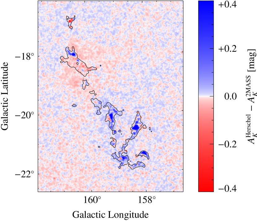
Figure 6: Difference between the extinction values evaluated with the 2MASS/NICEST map and the Herschel opacity map. The contour represents the $A_{K}=0.5\,\mathrm{mag}$ level.

4 Results

In order to characterize the maps, we produced the integral area function of the cloud, $S(>A_{\it{K}})$, i.e. the surface of the cloud above a certain extinction threshold as a function of that threshold. Lada et al. (2013) observed that the shape of the function $S(>A_{\it{K}})$ and of its derivative, $S^{\prime}(>A_{\it{K}})$, influences the variation in the rate of star formation of the cloud, especially in the high extinction regions.

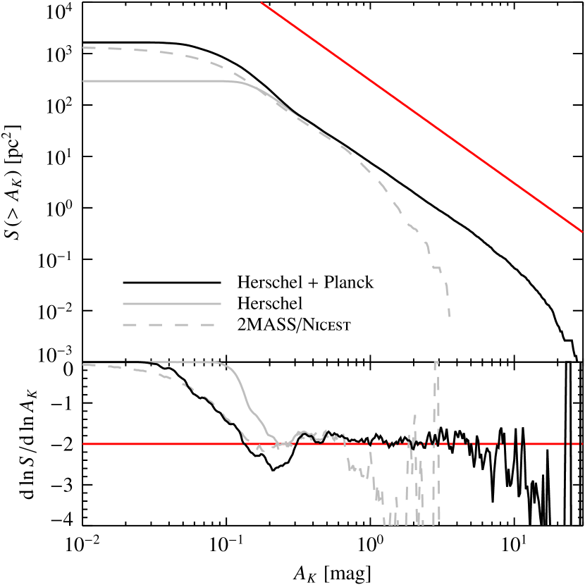
Figure 7: Integral area-extinction relation for Perseus, i.e., the physical cloud area above a given extinction threshold as a function of that threshold. The solid black line shows the result for the entire field, while the solid gray line shows the same quantity for the Herschel regions. The dashed line shows again the same quantity, but for the 2MASS/NICEST data. The red line shows the slope of the power law $S(>A_{K})\propto A_{K}^{-2}$.

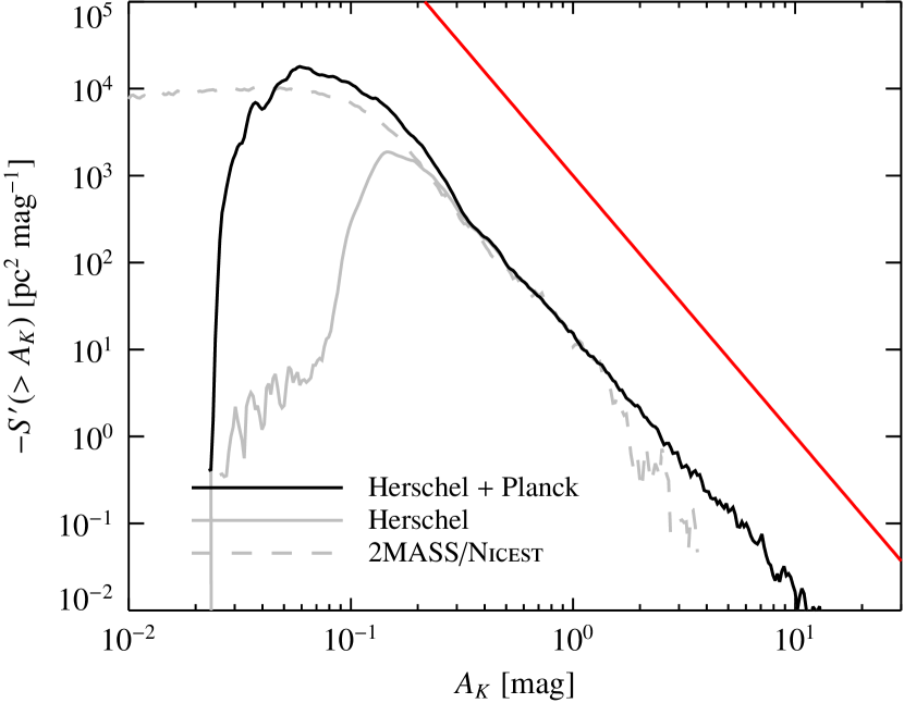
Figure 8: Function $-S^{\prime}(>A_{\it{K}})$, i.e. the probability distribution function of the measured column density for Perseus. In this plot a lognormal distribution would appear as a parabola, and a power law as a straight line. The red line shows the slope of the power law $S^{\prime}(>A_{K})\propto A_{K}^{-3}$.

The plot of $S\left(>A_{\it{K}}\right)$ is shown in Fig. 7 for different extinction measurements (Herschel, Herschel and Planck, 2MASS/NICEST). In the same figure, a red line with slope $-2$ is represented. Operationally, this plot is built by just counting the sky area above different values of $A_{K}$. As such, the specific spacing used for the threshold $A_{K}$ values is irrelevant (Fig. 7 we used a log-scale in $A_{K}$). The law $S(>A_{\it{K}})\propto A_{\it{K}}^{-2}$ appears to be an excellent description of the area function over two order of magnitudes, from $A_{K}\sim 0.1$ to $A_{K}\sim 10\,\mathrm{mag}$. The apparent break of this law at $A_{K}\sim$15\text{\,}\mathrm{m}\mathrm{a}\mathrm{g}$$ might either be genuine or due to systematic effects in the Herschel maps (unresolved structures, large temperature gradients, flux contamination from point sources). At the other extreme the break at $A_{K}<$0.15\text{\,}\mathrm{m}\mathrm{a}\mathrm{g}$$ can be due to various effects, including contamination by unrelated foreground and background material, and inappropriate definition of the cloud boundaries. In reality, as shown by Lombardi et al. (2015), fundamental constraints, such as contamination by unrelated foreground and background dust emission, severely limit our ability to measure the area function below $A_{K}<$0.15\text{\,}\mathrm{m}\mathrm{a}\mathrm{g}$$.

Fig. 8 shows $-S^{\prime}(>A_{\it{K}})$, as a function of $A_{\it{K}}$, where $A_{\it{K}}$ is evaluated through Eq. (4). This function is proportional to the probability distribution function (PDF) of the column density map and follows a power law with index equal to $-3$. Note that since we directly derived the function $S(>A_{K})$ using a 3-point Lagrangian interpolation (where the spacing $A_{K}$ is taken into account), this operation effectively produces a result that is proportional to a linearly-binned PDF. We stress that this differs from the choice adopted by Lombardi et al. (2015), where PDFs were logarithmically binned. Consequently, the slopes evaluated in this way differ by -1 to the one presented by Lombardi et al. (2015), but the results are equivalent.

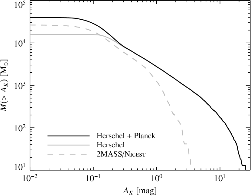
Figure 9: Integral mass-extinction relation, i.e. the cloud mass above a given extinction threshold. The line codes follow the same convention as in Fig. 7. The values of the mass above a certain extinction threshold are listed in Table 2

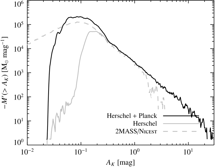
Figure 10: Function $-M^{\prime}(>A_{\it{K}})$, i.e. the derivative of the integral mass function.

Table 2: Mass values above an extinction threshold, normalized at the mass at $0.1\,\mathrm{mag}$, $M_{0.1}$.

$A_{K}[\mathrm{mag}]$	$M\,[\mathrm{M_{\odot}}]$	$M/M_{0.1}$
0.01	22153	168 %
0.1	13189	100 %
0.2	7864	60 %
0.4	4956	37 %
0.6	3685	27 %
0.8	2887	21 %
1.6	1532	11 %
3.2	777	5 %
6.4	341	2 %

Figs. 9 and 10 show the integral function of the mass $M(>A_{\it{K}})$ as a function of $A_{\it{K}}$ and its derivative $-M^{\prime}(>A_{\it{K}})$. The gas surface density, $\Sigma_{\mathrm{gas}}$, can be expressed as a mass surface density through the following relation:

$$\frac{\Sigma_{\mathrm{gas}}}{A_{\it{K}}}=\mu m_{p}\beta_{\it{K}}\simeq$183\text{\,}\mathrm{M_{$\odot$}}$\,\mathrm{{pc}^{-2}}\,\mathrm{mag^{-1}},$$ (9)

where $\mu=1.37$ is the mean molecular weight, corrected for the helium abundance, $m_{p}=1.67\times 10^{-24}\mathrm{g}$ is the proton mass and $\beta_{\it{K}}=1.67\times 10^{22}\mathrm{cm^{-2}mag^{-1}}=\left[2N\left(H_{2}\right)+N\left(H_{I}\right)\right]/A_{\it{K}}$ is the gas-to-dust ratio. The agreement between the solid line (Herschel and Planck data) and the dashed line (2MASS/NICEST) in Fig. 7 and Fig. 9 is good until $A_{\it{K}}\simeq 0.1\,\mathrm{mag}$, while the discrepancy we observe at high extinction values is due to the higher levels of extinction reached by Herschel. Similarly to Lombardi et al. (2014), we can define the mass of the cloud as the surface density integrated over the area:

$$M=\int\Sigma_{\mathrm{gas}}\,dS,$$ (10)

from which:

$$M\left(>A_{\it{K}}\right)\propto\int_{A_{\it{K}}}^{\infty}\frac{dS\left(>A^{\prime}_{\it{K}}\right)}{dA^{\prime}_{\it{K}}}A^{\prime}_{\it{K}}dA^{\prime}_{\it{K}}.$$ (11)

Notice how the power law trend observed in Fig. 9 is a direct consequence of the power law observed in Fig. 7, by replacing $dS(>A^{\prime}_{K})/dA^{\prime}_{K}$ with $A_{K}^{{}^{\prime}-3}$ in Eq. (11).

5 The local Schmidt law

Another possible application of the column density maps is to study the validity of the Schmidt law (Schmidt, 1959) in the Perseus molecular cloud. Half a century ago, Schmidt conjectured that the rate of star formation, $\Sigma_{\mathrm{SFR}}$ depends on the (projected) gas density, $\Sigma_{\mathrm{gas}}$, and in particular is a simple power law. Schmidt argued that the index of the power law was $\sim 2$. Recently, a series of observational studies (Lada (2014) and references therein) demonstrated, using observations of protostellar objects, that a Schmidt scaling law exists within a sample of nearby molecular clouds and it is typically characterized by an index $\sim 2$. In what follows we investigate the Schmidt law, using in particular Class I and Class 0 protostars to estimate the protostar surface density. Following Lada et al. (2013), we decided to consider only such sources, since they are likely still at or close to their original birth place. To estimate the protostar surface density, $\Sigma_{\mathrm{YSO}}$, we used already existing catalogs based on Spitzer data and we built a catalog of young stellar objects through the analysis of the WISE satellite data. We used the WISE data mainly to enhance and improve the Spitzer based catalogs. Indeed, even though WISE resolution (6.1”, 6.4”, 6.5”, and 12.0” in the four bands) is lower than Spitzer, its all-sky coverage allows to include sources detected in areas not surveyed by Spitzer. To make our classification as complete as possible, we also included the new sources detected by Sadavoy et al. (2014).

5.1 Identifying YSO candidates

The procedure adopted to search for YSO candidates is based on a comparison of the source distribution in several color-color diagrams between the science and a control field. We choose a control field in the region defined by:

$$137^{\circ}<l<147^{\circ}\hskip 14.22636pt-25^{\circ}<b<-15^{\circ}.$$ (12)

We selected this area based on two requirements: it is characterized by low extinction values and the background object distribution is similar to the one of the science field, since it has the same galactic latitude of the science field, which corresponds to the region defined previously for 2MASS data. To classify the sources in the science field, we approximately followed the scheme proposed by Koenig et al. (2012), which in turn is based on the scheme by Gutermuth et al. (2008) and Gutermuth et al. (2009). Koenig analysed several WISE color-color diagrams of Spitzer selected YSOs in the Taurus region. Besides, they characterized the contaminating sources by studying the distribution of objects with declination $>88^{\circ}.22$ (celestial north pole) in the $W_{1}-W_{2}$ vs. $W_{2}-W_{3}$ color-color diagram. By comparing the science and the control field color-color diagrams, one can note the presence in the science field of sources with color excess: these may be reddened background objects or embedded YSOs. As Rebull et al. (2011) noted, no color-color diagram can perfectly find all the YSOs and remove all the contaminants: the contamination rate for any color selection is expected to be large and ancillary data from other observations are often needed to choose the most likely candidates. Koenig et al. (2012) estimated a contamination rate for ”typical” star forming regions of about 2.4 objects resembling Class I YSOs, 3.8 objects resembling Class II YSOs, and 1.8 objects resembling transition discs per square degree. As a result, in our field, which is $\sim 100\,\mathrm{deg^{2}}$, the contaminants expected are respectively $\sim 240$, $\sim 380$, and $\sim 180$.

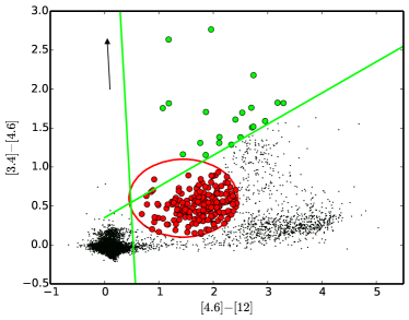
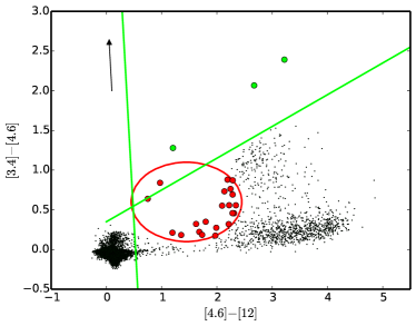
Figure 11: $W1-W2$ ($[3.4]-[4.6]$) vs. $W2-W3$ ($[4.6]-[12]$) diagram for the science and the control field. Red points represent candidate Class II objects, green points represent candidate Class I objects, while black points represent the other sources in the field. The red ellipse and the green lines have equations specified in the text.

Figure 11 shows the color-color diagram in $W_{1}$, $W_{2}$ and $W_{3}$ bands of the science (left) and the control field (right). Comparing them, we observed a significant excess of sources inside the marked red ellipse with center

$$\left\{\begin{aligned} \left[4.6\right]-\left[12\right]&=1.45\,\mathrm{mag},\\ \left[3.4\right]-\left[4.6\right]&=0.6\,\mathrm{mag}\end{aligned}\right.$$ (13)

and axes $a=1\,\mathrm{mag}$ and $b=0.5\,\mathrm{mag}$, and between the two blue slopes with equations:

$$\left\{\begin{aligned} \left[3.4\right]-\left[4.6\right]&=0.4\times\left([4.6]-[12]\right)+0.35\,\mathrm{mag},\\ \left[3.4\right]-\left[4.6\right]&=-12.4\times\left([4.6]-[22]\right)+6.3\,\mathrm{mag}.\end{aligned}\right.$$ (14)

Therefore, we primarily select 213 objects inside these two regions. The reddening of the objects inside the ellipse is low, and therefore we can suppose that they are Class II YSOs. Instead, the objects included between the two slopes (22) are highly reddened and can be classified as Class I protostars. We can observe that the selected Class I protostars satisfy Koenig requirements. Besides, our classification is stricter, since we remove all sources in the AGN/galaxy region of the diagram. Also the selection criteria of Class II YSOs are close to the ones chosen by Koenig et al. (2012). Indeed, the minimum color values accepted to include a source in the selection are:

$$\left\{\begin{aligned} \left[4.6\right]-\left[12\right]&=0.95\,\mathrm{mag},\\ \left[3.4\right]-\left[4.6\right]&=0.35\,\mathrm{mag}.\end{aligned}\right.$$ (15)

Figure 12 shows the diagrams $[3.4]-[4.6]$ vs. $[4.6]-[22]$ and is analogous to the previous one. Class II YSOs lie within the red ellipse, with center

$$\left\{\begin{aligned} \left[4.6\right]-\left[22\right]&=3\,\mathrm{mag},\\ \left[3.4\right]-\left[4.6\right]&=0.5\,\mathrm{mag},\end{aligned}\right.$$ (16)

and axes $a=2.5\,\mathrm{mag}$ and $b=0.5\,\mathrm{mag}$, while Class I protostars are included between the slopes with equations:

$$\left\{\begin{aligned} \left[3.4\right]-\left[4.6\right]&=0.4\times\left([4.6]-[22]\right)-0.3\,\mathrm{mag},\\ \left[3.4\right]-\left[4.6\right]&=1.3\times\left([4.6]-[22]\right)-1.2\,\mathrm{mag}.\end{aligned}\right.$$ (17)

The total number of sources is 130: 117 of them are classified as Class II YSOs, while the remaining 13 as Class I protostars. Further, we can observe the similarity with Koenig criteria.

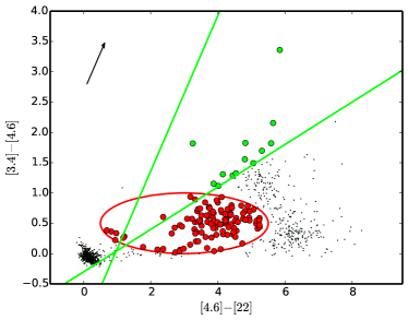
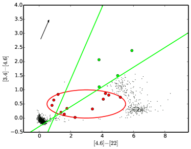
Figure 12: $W1-W2$ vs. $W2-W4$ diagram of the science and the control field. Red points represent candidate Class II YSOs, green points represent candidate Class I protostars, while black points represent the other sources in the field. The red ellipse and the green slopes have equations specified in the text.

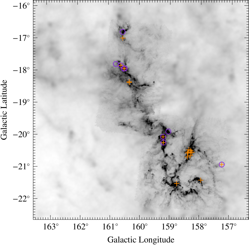
Figure 13: Spatial distribution of candidate Class I objects (orange crosses) selected through the $[3.4]-[4.6]$ vs. $[4.6]-[12]$ color-color diagram and Class I objects (purple circles) selected through the $[3.4]-[4.6]$ vs. $[4.6]-[22]$ color-color diagram. The map shown here is the optical depth map presented before.

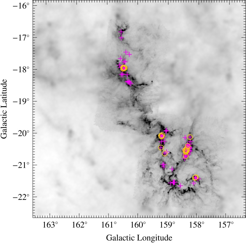
Figure 14: Spatial distribution of the candidate Class I (pink crosses) and Class 0 objects (orange circles, see Sadavoy et al. (2014)) used to estimate the Schmidt law.

To find YSO candidates associated with known objects, we cross-checked our selection with SIMBAD astronomical database and with the catalogs by Evans et al. (2009); Gutermuth et al. (2008, 2009); Jørgensen et al. (2006); Kirk & Myers (2011); Winston et al. (2009) and Young et al. (2015), based on Spitzer data. Many sources selected through WISE data analysis were already included in other catalogs. Nevertheless, the complete sky coverage of the WISE satellite allows to study regions that are parts of the cloud but were never observed by Spitzer. The final selection consists of previously identified Spitzer sources merged with newly identified WISE objects. 61 new sources were selected through WISE data, of which 17 belong to IC 348 and just one to NGC 1333.

We now focus on the candidate Class I protostars selected previously with our color-color diagrams. To further anlayse these sources, in particular to test whether our classification scheme is reliable, it is useful to study their spatial distribution. Figure 13 shows the positions of the Class I protostars that were selected through the $[3.4]-[4.6]$ vs. $[4.6]-[12]$ and $[3.4]-[4.6]$ vs. $[4.6]-[22]$ diagrams. All sources (except one) are placed in the highest opacity regions: this agrees well with the hypothesis that they are located close to their original place of formation. Most of Class I YSOs selected through the $[3.4]-[4.6]$ vs. $[4.6]-[12]$ diagram are situated in the NGC 1333 region. This could imply, as Jørgensen et al. (2006) observed, that the age of NGC 1333 is slightly lower than the age of IC 348: indeed, it is estimated that IC 348 is 2 Myrs old (Muench et al., 2007), while NGC 1333 does not exceed 1 Myr (Lada et al., 1996). We already noted that the number of sources selected with the $[3.4]-[4.6]$ vs. $[4.6]-[22]$ is lower than for the $[3.4]-[4.6]$ vs. $[4.6]-[12]$ diagram. Class I protostars in $[3.4]-[4.6]$ vs. $[4.6]-[12]$ diagram correspond to Class I protostars in $[3.4]-[4.6]$ vs. $[4.6]-[22]$ diagram, except for three sources not detected in the first diagram. Surprisingly, the $[3.4]-[4.6]$ vs. $[4.6]-[22]$ diagram does not detect any Class I protostar in NGC 1333. We evaluated the cloud temperature and optical depth at each object position. We excluded from the WISE selection all the objects in areas with optical depth $\tau<3.141\times 10^{-5}$ (corresponding to $A_{K}<0.1\,\mathrm{mag}$), supposing that this level of optical depth corresponds to the cloud boundaries. Figure 14 shows the final selection of Class I and Class 0 protostars (139 sources). Only 2 of the new sources selected by WISE are classified as Class I protostars. All the other sources in the figure have been previously classified using Spitzer data. We noted that for some sources our classification differs from the one obtained by Spitzer catalogs. In those cases, we decided to follow the Spitzer classification.

5.2 Determining the Schmidt law

We computed the extinction at each source position using our Herschel derived extinction map and binned them in log-spaced bins. Then we evaluated the cloud area between two consecutive extinction levels and the number of sources included within them. In this way, we evaluated the protostar surface density, $\Sigma_{\mathrm{YSO}}$, as a function of the extinction, as the number of sources between two consecutive extinction levels divided by the corresponding area. Since the gas surface density $\Sigma_{\mathrm{gas}}$ is proportional to the $K$ band extinction (see Eq. (9)), it is possible to express the Schmidt law as:

$$\Sigma_{\mathrm{YSO}}=\kappa A_{K}^{\beta},$$ (18)

where $\Sigma_{\mathrm{YSO}}$ is simply equal to $\Sigma_{\mathrm{SFR}}\times\tau$, and $\tau$ is the mean age of a Class I/0 protostar. Figure 15 represents the Schmidt law for the Perseus molecular cloud. The values obtained for the parameters are

$$\left\{\begin{aligned} \kappa&=0.2\pm 0.07\,\mathrm{[YSO\,pc^{-2}\,mag^{-\beta}]},\\ \beta&=2.4\pm 0.6.\end{aligned}\right.$$ (19)

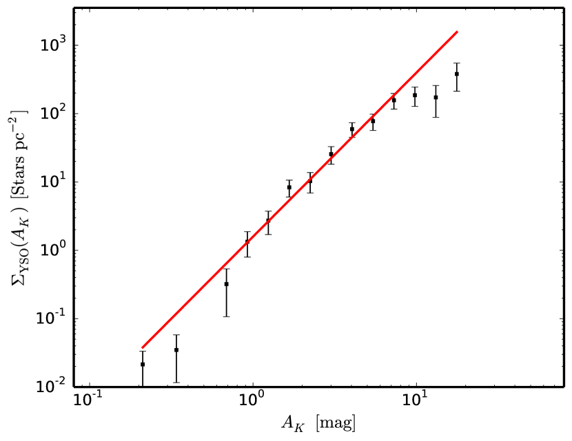
Figure 15: The Schmidt law in the Perseus molecular cloud. Here, $\Sigma_{\mathrm{YSO}}\propto A_{K}^{2.4}$, and $A_{K}\propto\Sigma_{\mathrm{gas}}$.

The value we found for $\beta$ is steeper (although compatible) than what reported by Lombardi et al. (2014) for the Orion molecular cloud complex and by Lada et al. (2013) for Taurus molecular cloud. Indeed, Lombardi et al. (2014) found $\beta=1.99\pm 0.05$ for Orion A and $\beta=2.16\pm 0.10$ for Orion B, while Lada et al. (2013) found $\beta=2.09\pm 0.14$ for Taurus. Even though the Schmidt law is a useful tool to understand the star formation inside the cloud, it does not completely describe the whole process. For this purpose, we considered the function that represents the cumulative number of sources above a certain extinction $A_{K}$ as a function of that extinction, shown in Fig. 16. Even though the Schmidt law predicts that the surface density of protostars steeply grows with extinction, the effective number of protostars decreases as the extinction increases, similarly to what is observed for the Orion molecular cloud in Lada et al. (2013).

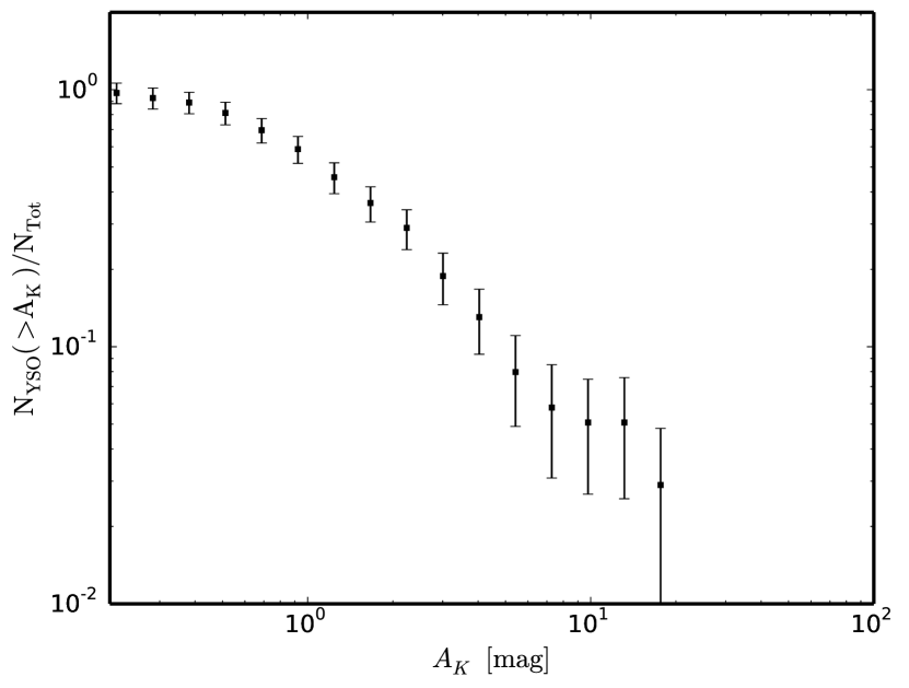
Figure 16: The cumulative protostellar function in the Perseus cloud as a function of $A_{K}$, i.e. $N_{\mathrm{YSO}}(>A_{K})$.

The total number of protostars is defined as (Lada et al., 2013):

$$N_{\mathrm{YSO}}=\int\Sigma_{\mathrm{YSO}}(A_{K})dS=\int\Sigma_{\mathrm{YSO}}(A_{K})\lvert S^{\prime}(>A_{K})\rvert dA_{K}.$$ (20)

Indeed, the number of protostars at a given extinction level is the product of the area $S(A_{K})$ encompassing that extinction level, and $\Sigma_{\mathrm{YSO}}(A_{K})$. The total number of protostars is given by the integral of this product over all extinction in the cloud. Changing the integration variable from $S$ to $A_{K}$ gives Eq. (20). We already studied the function $S(>A_{K})$ (Fig. 7) and we concluded that its trend is $\propto A_{K}^{-2}$ and therefore $S^{\prime}(>A_{K})\propto A_{K}^{-3}$. Thus, the number of protostars formed within the cloud does not depend only on the surface density of the gas but also on the area function and its derivative of the integral area function, i.e. the (unnormalized) PDF. As Lombardi et al. (2015) showed, the PDFs of a sample of nearby molecular clouds, including Perseus, follow roughly the same profile, with slopes in logarithmic binning between $\sim-2$ and $\sim-4$, which correspond to slopes between $\sim-3$ and $\sim-5$ in the linear binning that was done here. Therefore, it is conceivable to assume that, if the clouds have the same PDF and the same Schmidt law, then the function that describes the number of protostars above a certain extinction (normalized to the total number of protostars) is roughly the same for all the clouds.

6 Conclusions

Our main results are the following ones:

• We produced optical depth and temperature maps of the Perseus molecular cloud, obtained using the data from the Herschel and Planck satellites. The maps have a $36\,\mathrm{arsec}$ resolution for Herschel observations and a $5\,\mathrm{arcmin}$ resolution elsewhere.

• We calibrated the optical depth maps using 2MASS/NICEST extinction data and we obtained extinction maps at the resolution of Herschel with a dynamic range $1\times 10^{-2}\mathrm{mag}$ to $20\,\mathrm{mag}$ of $A_{K}$. In particular, we evaluated the ratio $C_{2.2}/\kappa_{850}=3620\pm 252$, i.e. the ratio between the $2.2\text{\,}\mathrm{\SIUnitSymbolMicro m}$ extinction coefficient and of the $850\text{\,}\mathrm{\SIUnitSymbolMicro m}$ opacity.

• We studied the cumulative and differential area functions of the data, and we showed that starting from $A_{K}\simeq 0.1\,\mathrm{mag}$ the cumulative area function follows a power law with index $\simeq-2$.

• We used WISE data to improve current YSO catalogs based mostly on Spitzer data and we built an up-to-date selection of Class I/0 protostars.

• We evaluated the local Schmidt law, $\Sigma_{\mathrm{YSO}}\propto A_{K}^{\beta}$, using the Herschel/Planck maps and the new object selection. We found that $\beta=2.4\pm 0.6$.

• We showed that the Schmidt law does not completely describe the whole star formation process. Indeed, the total number of protostars effectively formed within a cloud depends on the surface area function $S(>A_{K})$ and its derivative.

Appendix A Hidden layers of multiple layer figures

In this section we provide a ”flat” version of the hidden layers of multiple layer figures.

Figure 17: Error on the optical depth map (see fig. 3).

Figure 18: Error on the effective dust temperature map (see fig. 4).

Appendix B Potential new star cluster

It is worth mentioning that while analyzing the spatial distribution of the WISE excess sources, we noticed a small group slightly off-set from the cloud, whose center is located approximately at $l=162.2^{\circ},\,b=-19.4^{\circ}$. We found no reference in the literature regarding this potential new group of young stars. The group contains fourteen members spread across an area of about 1 square degree. None of the excess sources is present in the Hipparcos catalog, therefore it is not possible to give an estimate of its distance or its potential relation with the Perseus molecular cloud. Follow up observations for this new group of excess sources is needed. The Gaia mission is expected to dramatically improve the distance determination for faint stars, which will allow for a better understanding of the origins and relevance of this group to the history of the star formation in the Perseus region.

Appendix C Catalog of the sources used to evaluate the Schmidt law

In this section we provide the list of protostars used to evaluate the Schmidt law. We report the position for all the sources and the WISE magnitudes for the sources detected by both Spitzer and WISE.

Table 3: Catalog of the protostars used to determine the Schmidt law. Y15 stands for Young et al. (2015), G09 for Gutermuth et al. (2009), GMM09 for Gutermuth et al. (2008), E09 for Evans et al. (2009) and S14 for Sadavoy et al. (2014).

RA J2000 [deg]	DEC J2000 [deg]	W1 [mag]	W2 [mag]	W3 [mag]	W4 [mag]	Ref.
55.8726234	31.8720837	12.18 $\pm$ 0.03	10.55 $\pm$ 0.02	6.66 $\pm$ 0.02	7.5 $\pm$ 0.2	Y15
55.9000816	31.8358345					Y15
55.9382095	32.0662766					Y15
55.9625816	32.0522499					Y15
55.9868317	32.0513039					Y15
56.0109596	32.0331955					Y15
56.0383339	32.0438347	10.94 $\pm$ 0.04	9.66 $\pm$ 0.07	6.6 $\pm$ 0.1	7.1 $\pm$ 0.1	Y15
56.0540848	32.0265274					Y15
56.0889587	31.9923897					Y15
56.1035004	32.2301102					Y15
56.1262512	32.1931114					Y15
56.1805000	32.0254173	8.63 $\pm$ 0.03	6.93 $\pm$ 0.03	4.4 $\pm$ 0.07	8.5 $\pm$ 0.3	Y15
56.1831665	32.0267220					Y15
56.3075829	32.2027779					Y15
52.1356659	31.1847496	13.47 $\pm$ 0.04	11.88 $\pm$ 0.04	8.92 $\pm$ 0.07	8.0 $\pm$ NaN	Y15
52.1437073	31.0141945					Y15
52.1545410	31.2252235					Y15
52.1615829	31.3018322					Y15
52.1629181	31.1004734					Y15
52.1654587	31.2921944	11.43 $\pm$ 0.05	9.66 $\pm$ 0.04	6.96 $\pm$ 0.09	8.0 $\pm$ 0.3	Y15
52.1692924	31.2990265					Y15
52.1803322	31.2924709					Y15
52.2032089	31.2691116	13.50 $\pm$ 0.03	11.99 $\pm$ 0.03	9.2 $\pm$ 0.1	8.0 $\pm$ NaN	Y15
52.2135849	31.2942486					Y15
52.2314568	31.2435284					Y15
52.2358322	31.1269455					Y15
52.2383766	31.2386398					Y15
52.2434578	31.3715286					Y15
52.2467918	31.3423615					Y15
52.2471657	31.2635269					Y15
52.2522926	31.2002239					Y15
52.2565002	31.3390560					Y15
52.2638741	31.3873882					Y15
52.2657509	31.2677212	6.71 $\pm$ 0.06	4.93 $\pm$ 0.06	1.26 $\pm$ 0.01	-1.71 $\pm$ 0.002	Y15
52.2669182	31.2462502					Y15
52.2706261	31.3439999					Y15
52.2824173	31.3659172					Y15
52.2873764	31.3822498					Y15
52.2879181	31.3579731					Y15
52.2937088	31.2252789					Y15
52.2943764	31.2277775					Y15
52.2944984	31.3057213					Y15
52.2969170	31.3087215					Y15
52.2995415	31.3575001					Y15
52.3002510	31.2181664					Y15
52.3002510	31.2171402					Y15
52.3040428	31.3039722	10.38 $\pm$ 0.04	7.61 $\pm$ 0.09	5.65 $\pm$ 0.07	7.5 $\pm$ 0.15	Y15
52.3064156	31.2328339					Y15
52.3215408	31.4629173					Y15
52.3260841	31.3888607					Y15
52.3277931	31.3382511					Y15
52.3335838	31.4020824					Y15
52.3351669	31.3094997					Y15
52.3503761	31.3326683					Y15
51.3313332	30.5733891					Y15
51.3429985	30.7538605					Y15
51.4009171	30.7543602					Y15
51.4020424	30.7561665					Y15
51.4117928	30.7350559					Y15
51.4129982	30.7328339					Y15
51.6561241	30.2578049					Y15
51.9128342	30.2175274					Y15
51.9301262	30.2080288					Y15
51.9486237	30.2012501	7.4 $\pm$ 0.2	6.07 $\pm$ 0.03	3.46 $\pm$ 0.01	1.64 $\pm$ 0.02	Y15
52.0016251	30.1336937					Y15
52.1437073	31.0141945					Y15
52.1887512	31.0949726	13.81 $\pm$ 0.02	11.63 $\pm$ 0.02	8.89 $\pm$ 0.08	8.7 $\pm$ NaN	Y15
52.2752075	30.5108891					Y15
52.3478317	31.5581932					Y15
52.4659157	31.6516666					Y15
52.5630836	30.3970547					Y15
52.5935402	31.5445824					Y15
52.6130829	30.4749451	10.8 $\pm$ 0.03	9.94 $\pm$ 0.02	7.39 $\pm$ 0.04	7.4 $\pm$ 0.1	Y15
52.6361656	30.4407215					Y15
52.8112488	30.8320560	9.93 $\pm$ 0.03	8.82 $\pm$ 0.03	6.39 $\pm$ 0.07	6.0 $\pm$ 0.1	Y15
52.8374176	30.7583618					Y15
53.0748329	30.8298626					Y15
53.1215401	31.0446663					Y15
53.2410011	31.1023064					Y15
53.2767067	31.1346111					Y15
53.2898331	31.0920010					Y15
53.3035011	31.3567219	7.28 $\pm$ 0.04	5.73 $\pm$ 0.04	3.11 $\pm$ 0.01	0.93 $\pm$ 0.02	Y15
53.3074989	31.3348064					Y15
53.3099174	31.1196938					Y15
53.3185005	31.1145840					Y15
53.3193741	31.1320000					Y15
53.3243752	31.1588612					Y15
53.3346672	31.1226387	13.55 $\pm$ 0.02	10.19 $\pm$ 0.02	8.2 $\pm$ 0.1	8.7 $\pm$ NaN	Y15
53.3637085	31.1194992					Y15
55.4212074	31.8012772					Y15
55.4821243	31.8031654					Y15
55.4944572	31.8059444					Y15
55.5090408	31.8005829					Y15
55.7335434	31.9457760					Y15
56.1472511	32.4770012					Y15
56.7726250	32.7190285	9.6 $\pm$ 0.02	8.22 $\pm$ 0.02	5.72 $\pm$ 0.04	8.9 $\pm$ 0.5	Y15
56.9232483	32.8622475					Y15
52.1438332	31.1181946					G09
52.3001671	31.2172222					G09
52.3428345	31.2318058					G09
52.2390404	31.237833					G09
52.203167	31.2691383	13.50 $\pm$ 0.03	11.99 $\pm$ 0.03	9.25 $\pm$ 0.13	8.6 $\pm$ NaN	G09
52.1802902	31.2925282					G09
52.2034988	31.2982502					G09
52.237957	31.319973					G09
52.3048325	31.3303623					G09
52.2471237	31.3356113					G09
52.2705841	31.3440571					G09
52.2378769	31.3569717					G09
52.2872925	31.3823051					G09
52.3814163	31.4243889					G09
55.9001236	31.8358345					G09
56.0540848	32.0265274					G09
56.0098763	32.027916					G09
55.9965401	32.0474701					G09
55.9382095	32.0662766					G09
55.9778328	32.075695					G09
56.1262512	32.1931381					G09
56.2982101	32.4647789					G09
52.2416000	31.3478000					GMM09
52.2879000	31.3849000					GMM09
55.9791985	32.0175018					E09
55.9886017	32.0131989					E09
55.9855003	32.0147018					E09
55.9902	32.0124016					E09
55.9908981	32.0533981					E09
55.9975014	32.0098991					E09
55.9985008	32.0317001	7.5 $\pm$ 0.1	6.21 $\pm$ 0.03	4.10 $\pm$ 0.03	6.12 $\pm$ 0.05	E09
56.0890007	31.9923992					E09
55.5444984	31.7849007	13.09 $\pm$ 0.03	11.93 $\pm$ 0.05	10.48 $\pm$ 0.04	8.0 $\pm$ NaN	E09
53.196701	30.9878998	8.79 $\pm$ 0.02	7.64 $\pm$ 0.02	5.78 $\pm$ 0.08	8.0 $\pm$ NaN	E09
51.9094429	30.2329445	9.58 $\pm$ 0.02	8.27 $\pm$ 0.02	6.51 $\pm$ 0.03	8.7 $\pm$ 0.5	E09
51.3975	30.7589					S14
52.2575	31.2594					S14
52.3283	31.3867					S14
53.3387	31.1242					S14
51.2893562	30.7727299	8.43 $\pm$ 0.02	6.92 $\pm$ 0.02	4.2 $\pm$ 0.1	8.6 $\pm$ 0.5	New
55.5620079	31.7993259	13.94 $\pm$ 0.02	12.33 $\pm$ 0.03	9.92 $\pm$ 0.04	7.3 $\pm$ 0.2	New

References

- Andersson et al. (2000) Andersson, B.-G., Wannier, P. G., Moriarty-Schieven, G. H., & Bakker, E. J. 2000, AJ, 119, 1325
- André et al. (2010) André, P., Men’shchikov, A., Bontemps, S., et al. 2010, A&A, 518, L102
- Astropy Collaboration et al. (2013) Astropy Collaboration, Robitaille, T. P., Tollerud, E. J., et al. 2013, A&A, 558, A33
- Bachiller & Cernicharo (1984) Bachiller, R. & Cernicharo, J. 1984, A&A, 140, 414
- Bally et al. (2008) Bally, J., Walawender, J., Johnstone, D., Kirk, H., & Goodman, A. 2008, The Perseus Cloud, ed. B. Reipurth, 308
- Bigiel et al. (2008) Bigiel, F., Leroy, A., Walter, F., et al. 2008, AJ, 136, 2846
- Cernis (1990) Cernis, K. 1990, Ap&SS, 166, 315
- Cernis (1993) Cernis, K. 1993, Baltic Astronomy, 2, 214
- de Zeeuw et al. (1999) de Zeeuw, P. T., Hoogerwerf, R., de Bruijne, J. H. J., Brown, A. G. A., & Blaauw, A. 1999, AJ, 117, 354
- Enoch et al. (2006) Enoch, M. L., Sargent, A. I., Golwala, S., Evans, II, N. J., & Young, K. 2006, in Astronomical Society of the Pacific Conference Series, Vol. 357, Astronomical Society of the Pacific Conference Series, ed. L. Armus & W. T. Reach, 137
- Evans et al. (2009) Evans, N. J., Dunham, M. M., Jorgensen, J. K., et al. 2009, VizieR Online Data Catalog, 218, 10321
- Evans et al. (2014) Evans, II, N. J., Heiderman, A., & Vutisalchavakul, N. 2014, ApJ, 782, 114
- Griffin et al. (2010) Griffin, M. J., Abergel, A., Abreu, A., et al. 2010, aap, 518, L3
- Griffin et al. (2013) Griffin, M. J., North, C. E., Schulz, B., et al. 2013, MNRAS, 434, 992
- Gutermuth et al. (2009) Gutermuth, R. A., Megeath, S. T., Myers, P. C., et al. 2009, ApJS, 184, 18
- Gutermuth et al. (2008) Gutermuth, R. A., Myers, P. C., Megeath, S. T., et al. 2008, ApJ, 674, 336
- Gutermuth et al. (2011) Gutermuth, R. A., Pipher, J. L., Megeath, S. T., et al. 2011, ApJ, 739, 84
- Harvey et al. (2014) Harvey, P. M., Henning, T., Liu, Y., & Wolf, S. 2014, ApJ, 795, 21
- Hatchell et al. (2005) Hatchell, J., Richer, J. S., Fuller, G. A., et al. 2005, A&A, 440, 151
- Heiderman et al. (2010) Heiderman, A., Evans, II, N. J., Allen, L. E., Huard, T., & Heyer, M. 2010, ApJ, 723, 1019
- Herbig & Jones (1983) Herbig, G. H. & Jones, B. F. 1983, AJ, 88, 1040
- Hirota et al. (2008) Hirota, T., Bushimata, T., Choi, Y. K., et al. 2008, PASJ, 60, 37
- Jørgensen et al. (2006) Jørgensen, J. K., Harvey, P. M., Evans, II, N. J., et al. 2006, ApJ, 645, 1246
- Kennicutt (1998) Kennicutt, Jr., R. C. 1998, ApJ, 498, 541
- Kirk et al. (2006) Kirk, H., Johnstone, D., & Di Francesco, J. 2006, ApJ[astro-ph/0602089]
- Kirk & Myers (2011) Kirk, H. & Myers, P. C. 2011, ApJ, 727, 64
- Koenig et al. (2012) Koenig, X. P., Leisawitz, D. T., Benford, D. J., et al. 2012, ApJ, 744, 130
- Lada (2014) Lada, C. J. 2014, ArXiv e-prints [arXiv:1411.1053]
- Lada et al. (1996) Lada, C. J., Alves, J., & Lada, E. A. 1996, AJ, 111, 1964
- Lada et al. (2013) Lada, C. J., Lombardi, M., Roman-Zuniga, C., Forbrich, J., & Alves, J. F. 2013, ApJ, 778, 133
- Lombardi (2009) Lombardi, M. 2009, A&A, 493, 735
- Lombardi et al. (2015) Lombardi, M., Alves, J., & Lada, C. J. 2015, A&A, 576, L1
- Lombardi et al. (2014) Lombardi, M., Bouy, H., Alves, J., & Lada, C. J. 2014, A&A, 566, A45
- Lombardi et al. (2010) Lombardi, M., Lada, C. J., & Alves, J. 2010, A&A, 512, A67
- Lombardi et al. (2013) Lombardi, M., Lada, C. J., & Alves, J. 2013, A&A, 559, A90
- Mainzer et al. (2011) Mainzer, A., Bauer, J., Grav, T., et al. 2011, ApJ, 731, 53
- Muench et al. (2007) Muench, A. A., Lada, C. J., Luhman, K. L., Muzerolle, J., & Young, E. 2007, AJ, 134, 411
- Ott (2010) Ott, S. 2010, in Astronomical Society of the Pacific Conference Series, Vol. 434, Astronomical Data Analysis Software and Systems XIX, ed. Y. Mizumoto, K.-I. Morita, & M. Ohishi, 139
- Pezzuto et al. (2012) Pezzuto, S., Elia, D., Schisano, E., et al. 2012, A&A, 547, A54
- Planck Collaboration et al. (2014) Planck Collaboration, Abergel, A., Ade, P. A. R., et al. 2014, A&A, 571, A11
- Poglitsch et al. (2010) Poglitsch, A., Waelkens, C., Geis, N., et al. 2010, aap, 518, L2
- Rebull et al. (2011) Rebull, L. M., Koenig, X. P., Padgett, D. L., et al. 2011, ApJS, 196, 4
- Ridge et al. (2006) Ridge, N. A., Schnee, S. L., Goodman, A. A., & Foster, J. B. 2006, ApJ, 643, 932
- Sadavoy et al. (2012) Sadavoy, S. I., Di Francesco, J., André, P., et al. 2012, A&A, 540, A10
- Sadavoy et al. (2014) Sadavoy, S. I., Di Francesco, J., André, P., et al. 2014, ApJ, 787, L18
- Schlafly et al. (2014) Schlafly, E. F., Green, G., Finkbeiner, D. P., et al. 2014, ApJ, 786, 29
- Schmidt (1959) Schmidt, M. 1959, ApJ, 129, 243
- Skrutskie et al. (2006) Skrutskie, M. F., Cutri, R. M., Stiening, R., et al. 2006, AJ, 131, 1163
- Taylor (2005) Taylor, M. B. 2005, in Astronomical Society of the Pacific Conference Series, Vol. 347, Astronomical Data Analysis Software and Systems XIV, ed. P. Shopbell, M. Britton, & R. Ebert, 29
- Winston et al. (2009) Winston, E., Megeath, S. T., Wolk, S. J., et al. 2009, AJ, 137, 4777
- Wright et al. (2010) Wright, E. L., Eisenhardt, P. R. M., Mainzer, A. K., et al. 2010, AJ, 140, 1868
- Young et al. (2015) Young, K. E., Young, C. H., Lai, S.-P., Dunham, M. M., & II, N. J. E. 2015, The Astronomical Journal, 150, 40