The Euclidean quantisation of Kerr-Newman-de Sitter black holes

Abstract

We study the family of Einstein-Maxwell instantons associated with the Kerr-Newman metrics with a positive cosmological constant. This leads to a quantisation condition on the masses, charges, and angular momentum parameters of the resulting Euclidean solutions.

1 Introduction

Euclidean counterparts of Lorentzian solutions play an important role in Euclidean Quantum Gravity [HawkingInstantons, EQG]. It appears therefore of interest to find Euclidean versions of key Lorentzian solutions.

As such, Kerr-Newman solutions have a unique position in view of their uniqueness properties. The associated solutions with positive cosmological constant, discovered by Demiański and Plebański [PlebanskiDemianski] and, independently, by Carter [Carterseparable], are similarly expected to be unique under natural conditions. Surprisingly enough, their compact Euclidean counterparts do not seem to have been explored in the literature. The object of this paper is to fill this gap.

More precisely, we construct two new families of compact Riemannian four-dimensional manifolds satisfying the Einstein-Maxwell equations with a positive cosmological constant. The solutions are obtained by complex substitutions in the Kerr-Newman de Sitter metric. The requirement of smoothness and compactness of the underlying manifold leads to a quantisation condition on the mass and charge parameters of the associated Lorentzian manifold. We thus obtain our first family of metrics, on $S^{2}$- and ${\mathbbm{R}\mathbbm{P}^{2}}$-bundles over $S^{2}$, parameterised by two integers $(n_{1},n_{2})$. The second family is parameterised by a single integer $n\in\mathbb{N}$ and is obtained by passing to a limit à la Page in the Euclidean Kerr-Newman de Sitter metrics. We determine several physical parameters associated with the Lorentzian equivalents of the solutions and study their asymptotics as one, or both, parameters tend to infinity. We calculate the associated Euclidean actions, which determine the contribution of our instantons to the Euclidean path integral in a saddle point approximation, as well as horizon entropies and temperatures.

Our Riemannian solutions $(^{4}M,g)$ have a clear quantum relevance. On a more mundane level, since the Maxwell energy-momentum tensor has vanishing trace, the metrics we have constructed provide time-symmetric initial data for the $4+1$ vacuum Einstein equations with a positive cosmological constant, or for Einstein equations with matter (e.g., dust) having constant density on the initial data surface ${}^{4}M$. Indeed, the four-dimensional Euclidean Einstein-Maxwell equations imply that the four-dimensional Riemannian metric $g$ has constant positive scalar curvature. Therefore the initial data set $(^{4}M,g,K=0)$ satisfies the $4+1$ vacuum time-symmetric constraint equations with a positive cosmological constant, or $4+1$ time-symmetric constraint equations with dust which has constant density, or with a constant scalar field, or with a mixture of the above.

The solutions in our first family are uniquely parameterized by the already mentioned quantum numbers $(n_{1},n_{2})\in\mathbb{N}^{2}$, $1\leq n_{2}<n_{1}$, and the value of the cosmological constant $\Lambda$. It might be viewed as amusing, and perhaps not entirely unexpected, that after inserting the experimentally determined value of $\Lambda$, the masses of all Lorentzian solutions associated with our Euclidean ones are of the same order as some standard current estimates, based on the FLRW model, for the total mass of the visible universe.

The quantum numbers $(n_{1},n_{2})$, resulting from the requirement of regularity of the Riemannian manifold, lead to a quantisation of the mass, the angular momentum, and the combination $p^{2}-e^{2}$ of the magnetic charge parameter $p$ and electric charge parameter $e$. We show that the requirement of a well-defined test Dirac field with charge $q_{0}$ on the Riemannian manifold introduces two further quantum numbers $(\hat{n}_{1},\hat{n}_{2})$, together with a quantisation of $e$, $p$ and $q_{0}$.

2 The fields

The Kerr-Newman-de Sitter (KNdS) metric is a solution of the Einstein-Maxwell equations,

$$R_{\mu\nu}-\frac{1}{2}g_{\mu\nu}R+\Lambda g_{\mu\nu}=8\pi T_{\mu\nu}\,,~{}~{}~{}dF=0\,,~{}~{}~{}d\star F=0\,,$$ (2.1)

where $\Lambda$ is the cosmological constant (which we assume to be positive throughout this work), and where

$$T_{\mu\nu}=\frac{1}{4\pi}(F_{\mu\rho}F_{\nu}^{\phantom{\nu}\rho}-\frac{1}{4}F^{\alpha\beta}F_{\alpha\beta}g_{\mu\nu})\,.$$ (2.2)

In Boyer-Lindquist coordinates, after the replacement $a\rightarrow ia$, $t\rightarrow it$ and $e\rightarrow ie$ the metric takes the form

$$g = \frac{\Sigma}{\Delta_{r}}dr^{2}+\frac{\Sigma}{\Delta_{\theta}}d\theta^{2}+\frac{\sin^{2}(\theta)}{\Xi^{2}\Sigma}\Delta_{\theta}(a\mathrm{d}t+(r^{2}-a^{2})\mathrm{d}\varphi)^{2}$$ (2.3)

$$+\frac{1}{\Xi^{2}\Sigma}\Delta_{r}(dt-a\sin^{2}(\theta)\mathrm{d}\varphi)^{2}\,,$$

where, setting $\lambda=\Lambda/3$,

$$\Sigma=r^{2}-a^{2}\cos^{2}(\theta)\,,~{}~{}\Delta_{r}=(r^{2}-a^{2})\left(1-\lambda r^{2}\right)-2Mr+p^{2}-e^{2}\,,$$ (2.4)

$$\Delta_{\theta}=1-\lambda a^{2}\cos^{2}(\theta)\,,~{}~{}\Xi=1-\lambda a^{2}\,.$$ (2.5)

The Maxwell potential reads

$$A=\frac{p\,\cos(\theta)}{\Sigma}\sigma_{1}+\frac{e\,r}{\Sigma}\sigma_{2}\,,$$ (2.6)

where the one-forms $\sigma_{i}$, $i=1,2$, are defined as

$$\sigma_{1}=\frac{1}{\Xi}\left(-a\,\mathrm{d}t-(r^{2}-a^{2})\mathrm{d}\varphi\right)\,,\quad\sigma_{2}=\frac{1}{\Xi}\left(-\mathrm{d}t+a\sin^{2}(\theta)\mathrm{d}\varphi\right)\,.$$ (2.7)

Now, each metric (2.3) is determined uniquely by the parameters $a$, $M$, and the combination

$$p^{2}_{\textrm{eff}}:=p^{2}-e^{2}\,.$$ (2.8)

of the magnetic charge parameter $p$ and the electric charge parameter $e$. The notation in (2.8) might appear to be misleading, because the right-hand side of this equation could be negative. However, it turns out to be mostly appropriate, in that we have not found any non-singular solutions with $p^{2}\leq e^{2}$ using our procedure below except in the Page limit discussed in Appendix LABEL:s7IX15.1.

We emphasise that any pairs $(e,p)$ satisfying (2.8) are allowed. When transforming back to the Lorentzian regime, there is no ambiguity in determining the parameters $M$ and $a$ characterising the Lorentzian solution, which remain unchanged. On the other hand, if we denote by $p_{L}$ and $e_{L}$ the parameters characterising the Maxwell field on the Lorentzian side, then any values of $p_{L}$ and $e_{L}$ satisfying

$$p^{2}_{L}+e^{2}_{L}=p^{2}+e^{2}$$ (2.9)

are compatible with the Einstein-Maxwell equations for the Lorentzian metric. The question thus arises whether, given a set $(a,M,e,p)$ arising from a Riemannian metric, there is a preferred choice of $p_{L}$ and $e_{L}$.

A natural choice is

$$p_{L}=p\,,\quad e_{L}=e\,.$$ (2.10)

The condition ${p^{2}_{\textrm{eff}}}>0$ and (2.8) imply that the simplest choice $p_{L}=0$ in (2.10) is not possible, except in the Page limit. The next simplest choice, $e_{L}=0$, leads then to purely magnetic solutions with a quantised magnetic charge. We emphasise that our quantisation mechanism of magnetic charge has nothing to do with the Dirac one, see Section 7 below.

Whether or not (2.10) is the right choice appears to be a matter of debate, see [DunajskiTod1, HawkingRoss]. An alternative would be to decree that the Lorentzian solutions with $p_{L}=0$ and $e_{L}\neq 0$ correspond to Riemannian solutions for which $\hat{A}:={e_{L}\,r}\sigma_{2}/{\Sigma}$ is a vector potential for

$$\star F_{\mu\nu}:=\frac{1}{2}\epsilon_{\mu\nu}^{\phantom{\mu\nu}\alpha\beta}F_{\alpha\beta}=\partial_{\mu}\hat{A}_{\nu}-\partial_{\nu}\hat{A}_{\mu}\,,$$ (2.11)

where $\epsilon_{\mu\nu\alpha\beta}$ is the totally antisymmetric tensor. In this case $p^{2}_{\textrm{eff}}=e^{2}_{L}$ (compare [DunajskiTod1]). This choice leads to a quantisation of electric charge.

It might be of interest to note that planar Lorentz transformations of $(p,e)$ preserve $p^{2}_{\textrm{eff}}$, and can be thought of as the Euclidean counterparts of the usual duality transformations of the Maxwell field, which instead act as rotations of the $(p,e)$ plane.

In any case, we wish to find ranges of parameters so that (2.3) is a Riemannian metric on a closed manifold $M$. This leads to the following obvious restrictions:

First, compactness requires $\varphi$ and $t$ to be periodic, with a period which needs to be determined.

Further, compactness of $M$ requires a range of the variable $r$, bounded by two first-order zeros $r_{1}<r_{2}$ of $\Delta_{r}$, so that (2.3) is Riemannian for $\forall r\in(r_{1},r_{2}),\;\theta\in(0,\pi)$. In particular

$$\frac{\Sigma}{\Delta_{r}}>0~{}~{}~{}\text{and}~{}~{}~{}\frac{\Sigma}{\Delta_{\theta}}>0~{}~{}\forall r\in(r_{1},r_{2}),\;\theta\in(0,\pi).$$ (2.12)

Equations (2.4) and (2.5) show that $\Sigma$ and $\Delta_{\theta}$ are positive on the equatorial plane, and we conclude that

$$\Delta_{r}>0\,,~{}~{}~{}\Sigma>0~{}~{}~{}\text{and}~{}~{}~{}\Delta_{\theta}>0~{}~{}~{}\forall r\in(r_{1},r_{2}),\;\theta\in(0,\pi)\,.$$ (2.13)

Now, if $r_{1}r_{2}\leq 0$, then $0\in[r_{1},r_{2}]$, and since $\Sigma|_{r=0}<0$ this case will not lead to a regular Riemannian metric. Changing $r$ to its negative, it remains to consider the case where $0<r_{1}<r_{2}$. Positivity of $\Sigma$ leads then to $r_{1}>|a|$, and positivity of $\Delta_{\theta}$ imposes the restriction $\lambda^{-1}>a^{2}$. Summarising:

$$0<|a|<r_{1}<r_{2}\,,\quad a^{2}<\lambda^{-1}\,,\quad\Delta_{r}|_{(r_{1},r_{2})}>0\,.$$ (2.14)

Given a Euclidean metric as above with $e=0$, the corresponding Lorentzian metric with the same real values of $\lambda$, $M$, $a$, $e=0$, and $p$ will be called a partner solution. Note that the locations $r_{i}$ of the horizons of the partner solution will not coincide with the locations $r_{i}$ of the rotation axes of the associated Euclidean solutions; similarly for areas, surface gravities, etc.

3 Regularity at the rotation axes

For $r\in[r_{1},r_{2}]$ let us introduce two functions $\rho_{i}$, $i=1,2$, defined as

$$\rho_{i}=\epsilon_{i}\int_{r_{i}}^{r}\frac{1}{\sqrt{\Delta_{r}}}\mathrm{d}r=\frac{2}{\sqrt{\lambda_{i}}}\sqrt{\epsilon_{i}(r-r_{i})}\mathbb{1}_{1,i}(r-r_{i})\,,$$ (3.1)

with $\epsilon_{1}=1$, $\epsilon_{2}=-1$, and

$$\lambda_{i}:=\left|\Delta_{r}^{\prime}|_{r={r_{i}}}\right|\neq 0\,,\quad i=1,2\,,$$ (3.2)

and with functions $\mathbb{1}_{1,i}$ which are smooth near the origin and satisfy $\mathbb{1}_{1,i}(0)=1$. The function $\rho_{1}$ will serve as a coordinate replacing $r$ for $r\in[r_{1},r_{2})$, while $\rho_{2}$ will replace $r$ for $r\in(r_{1},r_{2}]$. Inverting, it follows that

$$r=r_{1}+\frac{\lambda_{1}}{4}\rho_{1}^{2}\mathbb{1}_{2}(\rho_{1}^{2})\,,\qquad\Delta_{r}=\frac{\lambda_{1}^{2}}{4}\rho_{1}^{2}\mathbb{1}_{3}(\rho_{1}^{2})\,,$$ (3.3)

with functions $\mathbb{1}_{2}$, $\mathbb{1}_{3}$ which are smooth near the origin, with $\mathbb{1}_{2}(0)=1=\mathbb{1}_{3}(0)$.

In order to make sure that the metric is regular near the intersection of the axes $\{\sin\theta=0\}$ with the axes $\{\Delta_{r}=0\}$, near $\theta=0$ and for $r\in[r_{1},r_{2})$ we use a coordinate system $(\rho_{1},t_{1},\theta,\phi_{1})$, with $t=\omega_{1}t_{1}$ and $\varphi$ defined through the formula

$$\mathrm{d}\varphi:=\alpha_{1}\mathrm{d}\phi_{1}+\frac{a}{a^{2}-r_{1}^{2}\color[rgb]{0,0,0}}\mathrm{d}t\equiv\alpha_{1}\mathrm{d}\phi_{1}+\frac{a\omega_{1}}{a^{2}-r_{1}^{2}\color[rgb]{0,0,0}}\mathrm{d}t_{1}\,,$$ (3.4)

for some constants $\alpha_{1},\omega_{1}\in\mathbb{R}^{*}$ which will be determined shortly by requiring $2\pi$-periodicity of $t_{1}$ and $\phi_{1}$. In (3.4) the coefficient in front of $\mathrm{d}t$ has been chosen so that $g_{tt}|_{\rho_{1}=0}=0$. In this coordinate system the metric takes the form

$$g = {\Sigma}\bigg{\{}\mathrm{d}\rho_{1}^{2}+\frac{1}{\Xi^{2}\Sigma^{2}}\bigg{[}\frac{\lambda_{1}^{2}\omega_{1}^{2}\Sigma^{2}}{4\left(r_{1}^{2}-a^{2}\color[rgb]{0,0,0}\right)^{2}}\mathbb{1}_{4}(\rho_{1}^{2},\sin^{2}(\theta))\rho_{1}^{2}\mathrm{d}t_{1}^{2}$$ (3.5)

$$\phantom{xx}+\alpha_{1}^{2}\big{(}\Delta_{\theta}\left(a^{2}-r^{2}\right)^{2}+a^{2}\Delta_{r}\sin^{2}(\theta)\big{)}\sin^{2}(\theta)\mathrm{d}\phi_{1}^{2}$$

$$\phantom{xx}+F(\rho^{2}_{1},\sin^{2}(\theta))\rho_{1}^{2}\sin^{2}(\theta)\mathrm{d}t_{1}\mathrm{d}\phi_{1}\bigg{]}+\frac{1}{\Delta_{\theta}}\mathrm{d}\theta^{2}\bigg{\}}\,,$$

for some smooth functions $\mathbb{1}_{4}$ and $F$, with $\mathbb{1}_{4}(0,y)=1$. As is well known, when $(\rho_{1},t_{1})$ are viewed as polar coordinates around $\rho_{1}=0$, the one form $\rho_{1}^{2}\mathrm{d}t_{1}$ and the quadratic form $\mathrm{d}\rho_{1}^{2}+\rho_{1}^{2}\mathrm{d}t_{1}^{2}$ are smooth. Similarly when $(\theta,\phi_{1})$ are polar coordinates around $\theta=0$, the one form $\sin^{2}(\theta)\mathrm{d}\phi_{1}$ and the quadratic form $\mathrm{d}\theta^{2}+\sin(\theta)^{2}\mathrm{d}\phi_{1}^{2}$ are smooth. It is then easily inferred that the requirements of $2\pi$-periodicity of $t_{1}$ and $\phi_{1}$, together with

$$\frac{\lambda_{1}^{2}\omega^{2}_{1}}{4\Xi^{2}\left(r_{1}^{2}-a^{2}\color[rgb]{0,0,0}\right)^{2}}=1\,,\quad\frac{\alpha_{1}^{2}\Delta_{\theta}^{2}\left(a^{2}-r^{2}\right)^{2}}{\Xi^{2}(r^{2}-a^{2}\cos^{2}(\theta))^{2}}\bigg{|}_{\theta=0}=1\,,$$ (3.6)

implies smoothness both of the sum of the diagonal terms of the metric $g$ and of the off-diagonal term $g_{t_{1}\phi_{1}}\mathrm{d}t_{1}\mathrm{d}\phi_{1}$ on

$$\{(r,t_{1},\theta,\phi_{1})\in[r_{1},r_{2})\times S^{1}\times[0,\pi)\times S^{1}\}\,.$$

Note that (3.6) is equivalent to

$$\omega_{1}=\pm\underbrace{\frac{2\Xi\left(r_{1}^{2}-a^{2}\right)}{\lambda_{1}}}_{=:\omega}\,,\quad\alpha_{1}=\pm 1\,.$$ (3.7)

The above calculations remain valid without changes near $\theta=\pi$. It is, however, convenient, to use a different symbol for the resulting polar coordinates: When $\theta\in(0,\pi]$ we will use $\hat{t}_{1}$ and $\hat{\phi}_{1}$ for the relevant angular coordinates, and $\hat{\omega}_{1}$, $\hat{\alpha}_{1}$ for the corresponding coefficients. Thus, for $\theta\in(0,\pi]$:

$$t=\hat{\omega}_{1}\hat{t}_{1}\,,\quad\mathrm{d}\varphi=\hat{\alpha}_{1}\mathrm{d}\hat{\phi}_{1}+\frac{a\hat{\omega}_{1}}{a^{2}-r_{1}^{2}\color[rgb]{0,0,0}}\mathrm{d}\hat{t}_{1}\,,$$ (3.8)

with

$$\hat{\omega}_{1}=\pm\omega\,,\quad\hat{\alpha}_{1}=\pm 1\,.$$ (3.9)

Identical considerations for $r\in(r_{1},r_{2}]$, using coordinate systems $(\rho_{2},t_{2}=t\omega_{2}^{-1},\theta,\phi_{2})$ for $\theta\in[0,\pi)$ and $(\rho_{2},\hat{t}_{2}=t\hat{\omega}_{2}^{-1},\theta,\hat{\phi}_{2})$ for $\theta\in(0,\pi]$, with

$$\mathrm{d}\varphi=\alpha_{2}\mathrm{d}\phi_{2}+\frac{a\omega_{2}}{a^{2}-r_{2}^{2}\color[rgb]{0,0,0}}\mathrm{d}t_{2}\,,\qquad\mathrm{d}\varphi=\hat{\alpha}_{2}\mathrm{d}\hat{\phi}_{2}+\frac{a\hat{\omega}_{2}}{a^{2}-r_{2}^{2}\color[rgb]{0,0,0}}\mathrm{d}\hat{t}_{2}\,,$$ (3.10)

lead to

$$\omega_{2}\,,\,\hat{\omega}_{2}\in\left\{\pm\frac{2\Xi\left(r_{2}^{2}-a^{2}\right)}{\lambda_{2}}\right\}\,,\quad\alpha_{2}\,,\,\hat{\alpha}_{2}\in\{\pm 1\}\,.$$ (3.11)

In an overlap region where both $t$ and $t_{1}$ are coordinates, the equation $t=\omega_{1}t_{1}$ implies that $t$ must be exactly $2\pi|\omega_{1}|$-periodic. Similarly, in any overlap region where both $t$ and $t_{2}$ are defined and are coordinates, $t$ must be exactly $2\pi|\omega_{2}|$-periodic. A similar argument applies to $\hat{t}_{i}$. So, the periodicity requirements of $t_{i}$ and $\hat{t}_{i}$ lead to

$$\omega_{1}=\pm\omega_{2}\,,\qquad\hat{\omega}_{1}=\pm\hat{\omega}_{2}\,.$$ (3.12)

3.1 $a=0$

When $a=0$, and imposing the regularity conditions above, the metric (3.13) simplifies considerably:

$$g = {r^{2}}\bigg{\{}\mathrm{d}\rho_{1}^{2}+\mathbb{1}_{4}(\rho_{1}^{2},\sin^{2}(\theta))\rho_{1}^{2}\mathrm{d}t_{1}^{2}+\mathrm{d}\theta^{2}+\sin^{2}(\theta)\mathrm{d}\phi_{1}^{2}\bigg{\}}\,.$$ (3.13)

The coordinate $\rho_{1}$ can be written explicitly in terms of elliptic integrals, which is not very enlightening.

After scaling to $\lambda=1$, the periodicity conditions (3.12) are verified by a one-parameter family of solutions parameterized by a continuous parameter ${p^{2}_{\textrm{eff}}}\in[0,1/16)$, see Figure 3.1. These solutions will not be discussed any further.

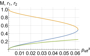
Figure 3.1: Solutions with $a=0$ scaled to $\lambda=1$. The uppermost curve is a plot of $r_{2}$, the middle one that of $r_{1}$, the lowest curve is a plot of the mass parameter $M$.

3.2 ${a\neq 0}$: the quantisation conditions

When $a\neq 0$, without loss of generality, replacing $t$ and/or $\varphi$ by their negatives if necessary, we require

$$a>0\,,\quad\omega_{1}=\omega>0\,.$$ (3.14)

To avoid ambiguities: except for the analysis of the Page limit in Appendix LABEL:s7IX15.1, in what follows we will assume that $(r,t,\theta,\varphi)$ form a smooth coordinate system away from the rotation axes, with $t$ and $\varphi$ periodic.

Increasing $\phi_{1}$ from zero to $2\pi$ with $(\rho_{1},t_{1},\theta)$ fixed takes one back to the starting point. Equations (3.4) and (3.7) show that $\varphi$ changes by $\pm 2\pi$, and therefore the minimal period of $\varphi$ must be $2\pi/k$ for some $k\in\mathbb{N}^{*}$. But then, increasing $\varphi$ from zero to $2\pi/k$ with $(r,t,\theta)$ fixed takes one to the same place. This results in an increase of $\phi_{1}$ by $\pm 2\pi/k$, which implies that $k=1$. Hence, $\varphi$ is exactly $2\pi$-periodic.

Now, increasing $t_{1}$ from zero to $2\pi$ with $\varphi_{1}$ fixed again takes one to the same place. This implies that $\varphi$ must have changed by an integer multiple of $2\pi$.

The same argument applies to $\varphi_{2}$ and $t_{2}$. We conclude that

$$n_{i}:=\frac{a\omega}{r_{i}^{2}-a^{2}}\in\mathbb{N}^{*}\,.$$ (3.15)

3.3 Maxwell fields

Let us check that the Maxwell fields, defined as $\mathrm{d}A$ away from all axes of rotation, extend by continuity to smooth fields once the above constraints have been imposed. This can be done by inspection of the Maxwell potentials (2.6) (which, incidentally, are not regular at the rotation axes).

We start with an analysis of the $p$-contribution to $A$ which, using (3.4) and its equivalent with $r_{1}$ replaced by $r_{2}$, can be rewritten as

$$\frac{p\,\cos(\theta)}{\Sigma}\sigma_{1}=\frac{p\,\cos(\theta)}{\Xi\Sigma}\left(-a\,\mathrm{d}t-(r^{2}-a^{2})\mathrm{d}\varphi\right)$$ (3.16)

$$=\frac{p\,\cos(\theta)}{\Xi\Sigma}\left(-a\,\mathrm{d}t-(r^{2}-a^{2})\left(\alpha_{i}\mathrm{d}\phi_{i}+\frac{a}{a^{2}-r_{i}^{2}\color[rgb]{0,0,0}}\mathrm{d}t\right)\right)$$

$$=\frac{p\,\cos(\theta)}{\Xi\Sigma}\left(\frac{a(r^{2}-r_{i}^{2})}{r_{i}^{2}-a^{2}}\,\mathrm{d}t-\alpha_{i}(r^{2}-a^{2})\mathrm{d}\phi_{i}\right)$$

$$=\underbrace{\frac{p\,\cos(\theta)}{\Xi}\left(\frac{a(r^{2}-r_{i}^{2})}{\Sigma(r_{i}^{2}-a^{2})}\,\mathrm{d}t+\frac{\alpha_{i}a^{2}\sin^{2}\theta}{r^{2}-a^{2}\cos^{2}(\theta)}\mathrm{d}\phi_{i}\right)}_{\text{\rm smooth}}-\frac{\alpha_{i}p\,\cos(\theta)}{\Xi}\mathrm{d}\phi_{i}\,,$$

where the index $i$ on $r_{i}$, $\alpha_{i}$ and $\phi_{i}$ takes the values $i\in\{1,2\}$. More precisely, the underbraced term in the last line of (3.16) is smooth away from $r=r_{2}$ when $i=1$, and away from $r=r_{1}$ when $i=2$. Near the axis $\cos\theta=1$ the last, non-smooth term can be rewritten as

$$-\frac{\alpha_{i}p\,\cos(\theta)}{\Xi}\mathrm{d}\phi_{i}=-\underbrace{\frac{\alpha_{i}p\,(\cos(\theta)-1)}{\Xi}\mathrm{d}\phi_{i}}_{\text{\rm smooth for $\theta<\pi$}}-\underbrace{\frac{\alpha_{i}p}{\Xi}\mathrm{d}\phi_{i}}_{\mathrm{closed}}\,,$$ (3.17)

which shows smoothness of the $p$-contribution to $F=\mathrm{d}A$ near $\theta=0$.

In fact, we have proved that, for $i=1,2$, the vector potentials

$$\frac{p\,\cos(\theta)}{\Sigma}\sigma_{1}+\frac{\alpha_{i}p}{\Xi}\mathrm{d}\phi_{i}=\frac{p\,\cos(\theta)}{\Sigma}\sigma_{1}+\frac{p}{\Xi}(\mathrm{d}\varphi-\frac{a}{a^{2}-r_{i}^{2}}\mathrm{d}t)$$ (3.18)

which are well-defined and smooth away from all axes of rotation, extend by continuity across $\theta=0$ and $r=r_{i}$ to smooth covector fields.

An identical calculation near the axis $\cos\theta=-1$, with $\phi_{i}$ replaced by $\hat{\phi}_{i}$, shows that the offending term can be rewritten as

$$-\frac{\alpha_{i}p\,\cos(\theta)}{\Xi}\mathrm{d}\hat{\phi}_{i}=-\underbrace{\frac{\alpha_{i}p\,(\cos(\theta)+1)}{\Xi}\mathrm{d}\hat{\phi}_{i}}_{\text{\rm smooth for $\theta>0$}}+\underbrace{\frac{\alpha_{i}p}{\Xi}\mathrm{d}\hat{\phi}_{i}}_{\mathrm{closed}}\,,$$ (3.19)

which finishes the proof of smoothness of the $p$-contribution to $F$ everywhere. We also see that the potentials

$$\frac{p\,\cos(\theta)}{\Sigma}\sigma_{1}-\frac{\alpha_{i}p}{\Xi}\mathrm{d}\hat{\phi}_{i}=\frac{p\,\cos(\theta)}{\Sigma}\sigma_{1}-\frac{p}{\Xi}(\mathrm{d}\varphi-\frac{a}{a^{2}-r_{i}^{2}}\mathrm{d}t)$$ (3.20)

extend smoothly to the axis $\theta=\pi$.

We continue with the $e$-contribution to $A$:

$$\frac{e\,r}{\Sigma}\sigma_{2}=\frac{e\,r}{\Sigma\Xi}\left(-\mathrm{d}t+a\sin^{2}(\theta)\mathrm{d}\varphi\right)=\frac{e\,r}{\Sigma\Xi}\left(-\mathrm{d}t+a\sin^{2}(\theta)\left(\alpha_{i}\mathrm{d}\phi_{i}+\frac{a}{a^{2}-r_{i}^{2}}\mathrm{d}t\right)\right)$$ (3.21)

$$= \frac{e\,r}{\Sigma\Xi}\left(\frac{r_{i}^{2}-a^{2}\cos^{2}(\theta)}{a^{2}-r_{i}^{2}}\mathrm{d}t+a\alpha_{i}\sin^{2}(\theta)\mathrm{d}\phi_{i}\right)$$

$$= \frac{e}{\Xi}\left(\frac{r_{i}^{2}-a^{2}\cos^{2}(\theta)}{r^{2}-a^{2}\cos^{2}(\theta)}\times\frac{r}{(a^{2}-r_{i}^{2})}\mathrm{d}t+\frac{\alpha_{i}ar\sin^{2}(\theta)}{r^{2}-a^{2}\cos^{2}(\theta)}\mathrm{d}\phi_{i}\right)$$

$$= \frac{e}{\Xi}\left(\left(1-\frac{r^{2}-r_{i}^{2}}{r^{2}-a^{2}\cos^{2}(\theta)}\right)\frac{r}{(a^{2}-r_{i}^{2})}\mathrm{d}t+\frac{\alpha_{i}ar\sin^{2}(\theta)}{r^{2}-a^{2}\cos^{2}(\theta)}\mathrm{d}\phi_{i}\right)$$

$$= \underbrace{\frac{e}{\Xi}\left(\frac{r-r_{i}}{(a^{2}-r_{i}^{2})}\mathrm{d}t-\frac{r^{2}-r_{i}^{2}}{r^{2}-a^{2}\cos^{2}(\theta)}\times\frac{r}{(a^{2}-r_{i}^{2})}\mathrm{d}t+\frac{\alpha_{i}ar\sin^{2}(\theta)}{r^{2}-a^{2}\cos^{2}(\theta)}\mathrm{d}\phi_{i}\right)}_{\text{\rm smooth near $r=r_{i}$}}$$

$$+\underbrace{\frac{er_{i}}{\Xi(a^{2}-r_{i}^{2})}\mathrm{d}t}_{\text{\rm closed}}\,.$$

This finishes the proof of smoothness of $F$.

Note that (3.21) shows that ${e\,r}\,\sigma_{2}/\Sigma$ extends smoothly across both $\theta=0$ and $\theta=\pi$ without further due as long as one stays away from the axes $r\in\{r_{1},r_{2}\}$.

4 Topology

The results of Section 3 can be summarised as follows: imposing $2\pi$-periodicity of $t_{1}$, $\hat{t}_{1}$, $t_{2}$, $\hat{t}_{2}$ $\varphi_{1}$, $\hat{\varphi}_{1}$, $\varphi_{2}$ and $\hat{\varphi}_{2}$, together with $\omega_{1}=\omega$, and $\hat{\omega}_{1}\,,\,\omega_{2}\,,\,\hat{\omega}_{2}\in\{\pm\omega\}$, as well as $\alpha_{1}$, $\hat{\alpha}_{1}\,,\,\alpha_{2}\,,\,\hat{\alpha}_{2}\in\{\pm 1\}$ and (3.15), the coordinates $(\rho_{i},t_{i},\theta,\varphi_{i})$, $(\rho_{i},\hat{t}_{i},\theta,\hat{\varphi}_{i})$, $i=1,2$ such that

$$\rho_{i}(r)=\int_{r_{i}}^{r}\frac{1}{\sqrt{\Delta_{r}}}\mathrm{d}r\,,\qquad\omega t_{1}=t=\pm\omega t_{2}\,,$$ (4.1)

$$\alpha_{1}\mathrm{d}\phi_{1}+\frac{a\omega}{r_{1}^{2}-a^{2}}\mathrm{d}t_{1}=\mathrm{d}\varphi=\alpha_{2}\mathrm{d}\phi_{2}\pm\frac{a\omega}{r_{2}^{2}-a^{2}}\mathrm{d}t_{2}\,,$$ (4.2)

similarly for the hatted ones, provide polar coordinates on the following four distinct coordinate patches, each containing exactly one intersection of the axes of rotation $\{\Delta_{r}=0\}\cap\{\sin(\theta)=0\}$ in their centers:

$$\Omega_{r_{1},0} := [r_{1},r_{2})_{\rho_{1}}\times S^{1}_{t_{1}}\times[0,\pi)_{\theta}\times S^{1}_{\phi_{1}}\approx D^{2}_{(\rho_{1},t_{1})}\times D^{2}_{(\theta,\phi_{1})}\,,$$ (4.3)

$$\Omega_{r_{2},0} := (r_{1},r_{2}]_{\rho_{2}}\times S^{1}_{t_{2}}\times[0,\pi)_{\theta}\times S^{1}_{\phi_{2}}\approx D^{2}_{(\rho_{2},t_{2})}\times D^{2}_{(\theta,\phi_{2})}\,,$$ (4.4)

$$\Omega_{r_{1},\pi} := [r_{1},r_{2})_{\rho_{1}}\times S^{1}_{\hat{t}_{1}}\times(0,\pi]_{\theta}\times S^{1}_{\hat{\phi}_{1}}\approx D^{2}_{(\rho_{1},\hat{t}_{1})}\times D^{2}_{(\theta,\hat{\phi}_{1})}\,,$$ (4.5)

$$\Omega_{r_{2},\pi} := (r_{1},r_{2}]_{\rho_{2}}\times S^{1}_{\hat{t}_{2}}\times(0,\pi]_{\theta}\times S^{1}_{\hat{\phi}_{2}}\approx D^{2}_{(\rho_{2},\hat{t}_{2})}\times D^{2}_{(\theta,\hat{\phi}_{2})}\,.$$ (4.6)

Here “$\approx$” means “diffeomorphic to”, and $D^{2}_{(\rho_{1},t_{1})}$ denotes an open disc $D^{2}\subset\mathbb{R}^{2}$ coordinatised by polar coordinates ${(\rho_{1},t_{1})}$ while $S^{1}_{t_{2}}$ denotes a circle $S^{1}$ coordinatised by $t_{2}$, etc. Quite generally, we use the notation $U_{x}$ to denote the fact that a set $U$ is coordinatised by a variable $x$.

The question then arises, in how many ways can one glue the sets above to obtain smooth closed manifolds. We point out some possible constructions here. While we suspect that these are all possibilities, we have not made in-depth attempts to analyse whether or not the list below is exhaustive. Note that oriented manifolds are obtained if and only if $\omega_{2}=\alpha_{1}\alpha_{2}\omega$.

1. We can glue $\Omega_{r_{1},0}$ with $\Omega_{r_{1},\pi}$ by identifying for $\theta\in(0,\pi)$ the points $(\rho_{1},t_{1},\theta,\varphi_{1})$ with $(\rho_{1},\hat{t}_{1},\theta,\hat{\varphi}_{1})$; similarly for $\Omega_{r_{2},0}$ and $\Omega_{r_{2},\pi}$. This corresponds to the choice $\alpha_{1}=\alpha_{2}$, and leads to the manifolds

   $$\widehat{\Omega}_{1}^{+}:=[r_{1},r_{2})_{\rho_{1}}\times S^{1}_{t_{1}}\times[0,\pi]_{\theta}\times S^{1}_{\phi_{1}}\approx D^{2}_{(\rho_{1},t_{1})}\times S^{2}_{(\theta,\phi_{1})}\,,$$

   as well as

   $$\widehat{\Omega}_{2}^{+}:=(r_{1},r_{2}]_{\rho_{2}}\times S^{1}_{t_{2}}\times[0,\pi]_{\theta}\times S^{1}_{\phi_{2}}\approx D^{2}_{(\rho_{2},t_{2})}\times S^{2}_{(\theta,\phi_{2})}\,,$$

   where $S^{2}$ denotes a two-dimensional sphere.

   Since the map $\theta\to\pi-\theta$ is an isometry, a second possibility in the same spirit is to identify for $\theta\in(0,\pi)$ the points $(\rho_{1},t_{1},\theta,\varphi_{1})$ with $(\rho_{1},\hat{t}_{1},\pi-\theta,\hat{\varphi}_{1}+\pi)$. This leads to ${\mathbbm{R}\mathbbm{P}^{2}}$ bundles over $D^{2}_{(\rho_{1},t_{1})}$ and $D^{2}_{(\rho_{2},t_{2})}$, which are not orientable.

2. Let us set

   $$\zeta:=\omega_{2}/\omega_{1}\in\{\pm 1\}\quad\Rightarrow\quad\mathrm{d}t_{1}=\zeta\mathrm{d}t_{2}\,.$$ (4.7)

   Consider the manifolds $\widehat{\Omega}_{i}^{+}$, $i=1,2$. Both are trivial $S^{2}$ bundles over the open disc $D^{2}$. Near the boundary of $D^{2}$, for each $t_{2}$ the corresponding sphere at $t_{1}$ is obtained by rotating $S^{2}$ around the $z$-axis by an angle $\alpha_{1}\zeta(n_{2}-n_{1})t_{2}$:

   $$\alpha_{1}\mathrm{d}\phi_{1}+n_{1}\mathrm{d}t_{1}=\alpha_{2}\mathrm{d}\phi_{2}+\zeta n_{2}\mathrm{d}t_{2}\quad\Longrightarrow\quad\phi_{1}=\alpha_{1}\alpha_{2}\phi_{2}+\alpha_{1}\zeta(n_{2}-n_{1})t_{2}+c\,,$$ (4.8)

   for some constant $c$. So, as we circle around the boundary of $D^{2}$, the sphere $S^{2}$ is rotated by a total angle $2\alpha_{1}\zeta(n_{2}-n_{1})\pi$ during each revolution. The end manifold is a non-trivial sphere bundle over $S^{2}$ when $n_{2}-n_{1}$ is odd.

   A similar construction applies to the ${\mathbbm{R}\mathbbm{P}^{2}}$ bundles above.

3. Let $(\rho_{1}){}_{\max}$ be the maximal value of the coordinate $\rho_{1}$, thus

   $$\rho_{1}(r) = \int_{r_{i}}^{r}\frac{1}{\sqrt{\Delta_{r}}}\mathrm{d}r=\underbrace{\int_{r_{1}i}^{r_{2}}\frac{1}{\sqrt{\Delta_{r}}}\mathrm{d}r}_{=(\rho_{1}){}_{\max}}-\underbrace{\int_{r}^{r_{2}}\frac{1}{\sqrt{\Delta_{r}}}\mathrm{d}r}_{=\rho_{2}}$$ (4.9)

   $$= (\rho_{1}){}_{\max}-\rho_{2}\,,\qquad$$

   and suppose that the map

   $$(\rho_{1}=\rho,t_{1}=s)\mapsto(\rho_{1}=(\rho_{1}){}_{\max}-\rho,t_{1}=s+\pi)$$

   is an isometry. This, however, occurs for the metrics considered here only in the Page limit, and is therefore only relevant to Appendix LABEL:s7IX15.1. Then the identification of $(\rho_{1},t_{1},\theta,\phi_{1})$ with

   $$(\rho_{2}=(\rho_{1}){}_{\max}-\rho_{1},\hat{t}_{2}=t_{1}+\pi,\pi-\theta,n(\phi_{1}+\pi))$$

   leads to a smooth compact manifold.

5 The solutions

The question then arises to find values of $(M,{p^{2}_{\textrm{eff}}},a)$ so that

$$\omega_{1}=\zeta\omega_{2}\,,\quad\zeta\in\{\pm 1\}\,,\quad\frac{a\omega_{1}}{r_{1}^{2}-a^{2}}=n_{1}\in\mathbb{N}^{*}\,,\quad\frac{a|\omega_{2}|}{r_{2}^{2}-a^{2}}=n_{2}\in\mathbb{N}^{*}\,.$$ (5.1)

It follows from (3.7) and (3.11) that the above equations are equivalent to

$$\frac{(r_{1}^{2}-a^{2})}{(r_{2}^{2}-a^{2})}\frac{\Delta^{\prime}_{r}(r_{2})}{\Delta^{\prime}_{r}(r_{1})}=-1\,,\quad\Delta^{\prime}_{r}(r_{1})n_{1}=2a\Xi\,,\quad-\Delta^{\prime}_{r}(r_{2})n_{2}=2a\Xi\,.$$ (5.2)

In addition we need to fulfill $\Delta_{r}(r_{i})=0$, leading to the system of polynomial equations for $(r_{1},r_{2},n_{1},n_{2},a,M,{p^{2}_{\textrm{eff}}})$.

$$\Delta_{r}(r_{1}) = 0\,,$$ (5.3)

$$\Delta_{r}(r_{2}) = 0\,,$$ (5.4)

$$\Delta^{\prime}_{r}(r_{1})n_{1}-2a\Xi = 0\,,$$ (5.5)

$$-\Delta^{\prime}_{r}(r_{2})n_{2}-2a\Xi = 0\,,$$ (5.6)

$$(r_{1}^{2}-a^{2})n_{1}-(r_{2}^{2}-a^{2})n_{2} = 0\,.$$ (5.7)

Note that $n_{1}>n_{2}\geq 1$ in view of (5.7). Moreover the solutions have to satisfy the constraints

$i)\phantom{ii}~{}M\in\mathbb{R}$, $a>0$, ${p^{2}_{\textrm{eff}}}\in\mathbb{R}$;

$ii)\phantom{i}~{}n_{1},n_{2}\in\mathbb{N}^{*}$;

$iii)~{}0<r_{1}<r_{2}$, $|a|<|r_{1}|$ and $a^{2}<\lambda^{-1}$.

We note that we also need $\forall r\in(r_{1},r_{2}):\Delta_{r}(r)>0$, but this follows from the fact that $\Delta^{\prime}_{r}(r_{1})$ is positive by (5.5) and $\Delta^{\prime}_{r}(r_{2})$ is negative by (5.6).

We also note that equations (5.3)-(5.7) involve neither $\zeta$ nor the $\alpha_{i}$’s as in (4.7)-(4.8), which can thus be arbitrarily chosen once a solution has been found.

Our strategy is to prescribe $\lambda\in\mathbb{R}_{+}^{*}$,$~{}n_{1},n_{2}\in\mathbb{N}^{*}$ so that (5.3)-(5.7) become a system of five polynomials in the variables $(r_{1},r_{2},{p^{2}_{\textrm{eff}}},M,a)$. We use Mathematica to compute a Gröbner basis of the system. This provides a simpler equivalent system to solve. It turns out that one is led to a hierarchic system of polynomial equations, the first one depending only on ${p^{2}_{\textrm{eff}}}$, the second one only on ${p^{2}_{\textrm{eff}}}$ and $a$, and so forth. An example is provided in Appendix A.

Our Mathematica calculations show the following: Let

$$n_{\max{}}=50\,.$$ (5.8)

Then:

1. There exist no solutions with $(n_{1},n_{2})\in\mathbb{N}\times\mathbb{N}$ with $1\leq n_{2}<n_{1}\leq n_{\max{}}$ and ${p^{2}_{\textrm{eff}}}\leq 0$. In particular there are no vacuum solutions with the properties set forth above.

2. For every pair $(n_{1},n_{2})\in\mathbb{N}\times\mathbb{N}$ with $1\leq n_{2}<n_{1}\leq n_{\max{}}$ there exists exactly one solution satisfying our constraints.

3. The physical parameters (see Appendix B) of the Lorentzian partner solutions are all bounded, cf. Table 5.1. In particular the physical mass of the Lorentzian partners is strictly positive, bounded away from zero, and bounded from above.

	$(n_{1},n_{2})_{\min{}}$	min.
${|{q}_{\textrm{phys}}|}{}$	$(2,1)$	0.2511
$M_{\textrm{phys}}$	$(\infty,1)$	0.2036
$|J_{\textrm{phys}}|$	$(2,1)$	0.01392
$S$	$(2,1)$	-2.357

	$(n_{1},n_{2})_{\max{}}$	max.
${|{q}_{\textrm{phys}}|}{}$	$(\infty,\infty)$	$\frac{\sqrt{2}}{3}\approx 0.47$
$M_{\textrm{phys}}$	$(100,90)$	0.2548
$|J_{\textrm{phys}}|$	$(\infty,\infty)$	$\frac{1}{9}\approx 0.111$
$S$	$(\infty,n_{2})$	$\infty$

Table 5.1: Left table: Minimal values of the effective physical Lorentzian charge ${|{q}_{\textrm{phys}}|}{}$, the physical mass $M_{\textrm{phys}}$, the physical angular momentum $|J_{\textrm{phys}}|$, and the Euclidean action $S$ with the corresponding quantum numbers $(n_{1},n_{2})_{\min{}}$. Right table: Maximal values of ${|{q}_{\textrm{phys}}|}{}:=\sqrt{{p^{2}_{\textrm{eff}}}}/(1+a^{2})$, $M_{\textrm{phys}}$, $|J_{\textrm{phys}}|$, $S$ with the corresponding quantum numbers $(n_{1},n_{2})_{\max{}}$. All values scaled to $\lambda=1$; compare Appendix D.

It should be emphasised that the existence of the solutions of the system as above is a rigorous result, derived by exact computer algebra. While numerics is used to check whether the joint zeros of the Gröbner basis satisfy the desired inequalities, this is again a rigorous statement, as the numerical errors introduced when checking the inequalities are well below the gaps occurring in the inequalities.

We expect that the threshold (5.8) is irrelevant, and indeed we have randomly sampled many further values of $(n_{1},n_{2})$, including e.g.

$$(n_{2},n_{1})\in\{(1,10000),(20,1000),(200,1000),(1000,10000)\}\,,$$

with the same result. Plots displaying various correlations between parameters are shown in Figure 5.1.

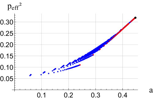
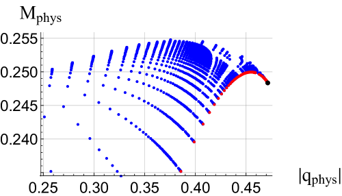
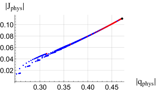
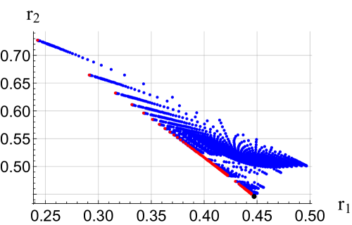
Figure 5.1: Correlations between $a$ and ${p^{2}_{\textrm{eff}}}$ (upper left plot), ${|{q}_{\textrm{phys}}|}{}$ and $M_{\textrm{phys}}$ (upper right), ${|{q}_{\textrm{phys}}|}$ and $|J_{\textrm{phys}}|$ (lower left), and $r_{1}$ vs. $r_{2}$ (lower right plot). The blue dots correspond to about 2000 solutions which are obtained by taking all values of $1\leq n_{2}<n_{1}\leq 50$ and a sample of values in the range $1\leq n_{2}<n_{1}\leq 1000$. The red dots are obtained by letting $n_{1}\to\infty$ (cf. Section 6), with $1\leq n_{2}\leq 9900$. The black dot is the limit $n_{1}\to\infty$, $n_{2}\to\infty$ (cf. Section 6).

The plots show that the resulting parameters $(a,M,{p^{2}_{\textrm{eff}}})$ are bounded, and that the values of the parameters approach affine correlations as both $n_{1}$ and $n_{2}$ tend to infinity. This is explained in Section 6 below, where exact bounds and the asymptotically affine relations are derived.

6 The limit $n_{1}\to\infty$

An interesting case arises when we require $r=a$ to be a double zero of $\Delta_{r}$. While in this case the geometry is not compact anymore, the resulting manifold provides a description of the geometry which is approached when $n_{1}$ tends to infinity with $n_{2}$ kept fixed. The values of the parameters $(a,m,{p^{2}_{\textrm{eff}}})$ which arise in this case correspond to the limiting curves which arise in the plots showing the correlations between the parameters.

In order to study the system (5.3-5.7) for large $n_{1}$, we rewrite (5.7) in the form

$$(r_{1}^{2}-a^{2})-(r_{2}^{2}-a^{2})\frac{n_{2}}{n_{1}} = 0\,.$$ (6.1)

Passing to the limit $n_{1}\rightarrow\infty$ with $n_{2}$ fixed one is led to

$$0=r_{1}^{2}-a^{2}=\Delta^{\prime}_{r}(r_{1})=\Delta_{r}(r_{1})=\Delta_{r}(r_{2})=-\Delta^{\prime}_{r}(r_{2})n_{2}-2a\Xi\,.$$ (6.2)

In particular $r_{1}=a$. Scaling the metric by a constant so that $\Lambda=3$, and using $r_{1}=a$ in Eq.(5.5) we obtain $M=a(1-a^{2})$. Injecting in (5.3) gives $p^{2}_{\textrm{eff}}{}=2a^{2}(a^{2}-1)$. Summarising

$$r_{1}=a\,,\qquad M=a(1-a^{2})\,,\qquad p^{2}_{\textrm{eff}}{}=2a^{2}(1-a^{2})\,.$$ (6.3)

The parameter $a$ can then be determined using

$$\Delta_{r}(r_{2})=0=\Delta^{\prime}_{r}(r_{2})n_{2}+2a\Xi\,,$$ (6.4)

with $M$ and $p^{2}_{\textrm{eff}}{}$ given by (6.3). Some algebra gives

$$a = \sqrt{\frac{2n_{2}\left(5n_{2}-2\sqrt{8n_{2}+1}+4\right)-\sqrt{8n_{2}+1}+1}{2n_{2}(25n_{2}+8)+2}}\,,$$ (6.5)

$$r_{2} = \frac{\left(2n_{2}+\sqrt{8n_{2}+1}+1\right)\sqrt{\frac{4n_{2}\left(5n_{2}-2\sqrt{8n_{2}+1}+4\right)-2\sqrt{8n_{2}+1}+2}{n_{2}(25n_{2}+8)+1}}}{4n_{2}}\,.$$ (6.6)

The corresponding physical parameters are

$$M_{\textrm{phys}}=\frac{a(1-a^{2})}{(1+a^{2})^{2}}\,,\qquad|J_{\textrm{phys}}|=\frac{a^{2}(1-a^{2})}{(1+a^{2})^{2}}\,,\qquad{|{q}_{\textrm{phys}}|}=\frac{a\sqrt{2(1-a^{2})}}{(1+a^{2})}\,.$$ (6.7)

Here $M_{\textrm{phys}}=M/(1+\lambda a^{2})^{2}$ is the physical mass of the Lorentzian partner solution (compare [GomberoffTeitelboim, CJKKerrdS]), $|J_{\textrm{phys}}|=aM/(1+\lambda a^{2})$ is the Komar angular momentum of the Lorentzian partner solution, and ${|{q}_{\textrm{phys}}|}:={\sqrt{{p^{2}_{\textrm{eff}}}}}/{(1+\lambda a^{2})}$ is the total magnetic Maxwell charge of the Lorentzian solution with $e=0$ (compare [Sekiwa]).

We have

$$\Delta_{r}^{\prime\prime}|_{r=a}=2-10a^{2}\,,$$

so that $\Delta_{r}$ is positive for $0<a<r_{2}$, with a simple zero at $r=r_{2}$, if and only if

$$0<a<\frac{1}{\sqrt{5}}\,.$$ (6.8)

Inspection of (2.3) shows that the metric $g$ is complete, with a smooth axis of rotation at the other zero $r=r_{2}$ of $\Delta_{r}$ when $n_{2}\in\mathbb{Z}$. The set $r=a$ is infinitely far away, with the region $r\to a$ displaying an interesting geometry: While the circles of constant $t$, $r$ and $\theta\not\in\{0,\pi\}$ shrink to zero as $r$ tends to $a$, the metric on the spheres of constant $\varphi$ and $r$ is stretched along the meridians and approaches a smooth Riemannian metric on a cylinder obtained by removing the north and south pole from $S^{2}$.

We have the following expansions, for large $n_{2}\in\mathbb{N}$,

$$a = \sqrt{\frac{2n_{2}\left(5n_{2}-2\sqrt{8n_{2}+1}+4\right)-\sqrt{8n_{2}+1}+1}{2n_{2}(25n_{2}+8)+2}}$$ (6.9)

$$= \frac{1}{\sqrt{5}}-\frac{2}{5}\sqrt{\frac{2}{5}}\sqrt{\frac{1}{n_{2}}}+\frac{2}{25\sqrt{5}n_{2}}+\frac{7}{100\sqrt{10}}\left(\frac{1}{n_{2}}\right)^{3/2}+O\left({n_{2}}^{-2}\right)\phantom{xxxx}$$

$$\to_{n_{2}\to\infty}\frac{1}{\sqrt{5}}\approx 0.45\,,$$

$$M = \sqrt{\frac{\left(2n_{2}\left(5n_{2}-2\sqrt{8n_{2}+1}+4\right)-\sqrt{8n_{2}+1}+1\right)}{8(n_{2}(25n_{2}+8)+1)^{3}}}\times$$ (6.10)

$$\phantom{xxxx}\times\left(4n_{2}\left(10n_{2}+\sqrt{8n_{2}+1}+2\right)+\sqrt{8n_{2}+1}+1\right)$$

$$= \frac{4}{5\sqrt{5}}-\frac{4}{25}\sqrt{\frac{2}{5}}\sqrt{\frac{1}{n_{2}}}-\frac{4}{25\sqrt{5}n_{2}}+\frac{39}{250\sqrt{10}}\left(\frac{1}{n_{2}}\right)^{3/2}+O\left({n_{2}}^{-2}\right)$$

$$\to_{n_{2}\to\infty}\frac{4}{5\sqrt{5}}\approx 0.36\,,$$

$${p^{2}_{\textrm{eff}}} = \frac{n_{2}^{2}\left(4n_{2}\left(50n_{2}-15\sqrt{8n_{2}+1}+34\right)-15\sqrt{8n_{2}+1}+17\right)}{(n_{2}(25n_{2}+8)+1)^{2}}$$ (6.11)

$$= \frac{1}{\sqrt{5}}-\frac{2}{5}\sqrt{\frac{2}{5}}\sqrt{\frac{1}{n_{2}}}+\frac{2}{25\sqrt{5}n_{2}}+\frac{7}{100\sqrt{10}}\left(\frac{1}{n_{2}}\right)^{3/2}+O\left({n_{2}}^{-2}\right)$$

$$\to_{n_{2}\to\infty}\frac{8}{25}\approx 0.32\,,$$

$$M_{\textrm{phys}} = \frac{4n_{2}\left(10n_{2}+\sqrt{8n_{2}+1}+2\right)+\sqrt{8n_{2}+1}+1}{\left(4n_{2}\left(-15n_{2}+\sqrt{8n_{2}+1}-6\right)+\sqrt{8n_{2}+1}-3\right)^{2}}$$ (6.13)

$$\times\sqrt{2(n_{2}(25n_{2}+8)+1)\left(2n_{2}\left(5n_{2}-2\sqrt{8n_{2}+1}+4\right)-\sqrt{8n_{2}+1}+1\right)}\phantom{xxxxx}$$

$$= \frac{\sqrt{5}}{9}+\frac{1}{27}\sqrt{\frac{2}{5}}\sqrt{\frac{1}{n_{2}}}-\frac{1}{5\sqrt{5}n_{2}}+\frac{421\left(\frac{1}{n_{2}}\right)^{3/2}}{48600\sqrt{10}}+\frac{8867}{145800\sqrt{5}n_{2}^{2}}-O\left({n_{2}}^{-5/2}\right)$$

$$\to_{n_{2}\to\infty}\frac{\sqrt{5}}{9}\approx 0.25\,,$$

$$|J_{\textrm{phys}}| = \frac{8n_{2}^{2}}{4n_{2}\left(18n_{2}+3\sqrt{8n_{2}+1}+10\right)+3\sqrt{8n_{2}+1}+5}$$ (6.15)

$$= \frac{1}{9}-\frac{1}{27}\sqrt{2}\sqrt{\frac{1}{n_{2}}}-\frac{1}{27n_{2}}+\frac{83}{1944\sqrt{2}}\left(\frac{1}{n_{2}}\right)^{3/2}+\frac{37}{5832n_{2}^{2}}+O\left(n_{2}^{-5/2}\right)$$

$$\to_{n_{2}\to\infty}\frac{1}{9}\,,$$

$${|{q}_{\textrm{phys}}|}{} = \frac{2(n_{2}(25n_{2}+8)+1)}{4n_{2}\left(15n_{2}-\sqrt{8n_{2}+1}+6\right)-\sqrt{8n_{2}+1}+3}$$ (6.17)

$$\times\sqrt{\frac{n_{2}^{2}\left(4n_{2}\left(50n_{2}-15\sqrt{8n_{2}+1}+34\right)-15\sqrt{8n_{2}+1}+17\right)}{(n_{2}(25n_{2}+8)+1)^{2}}}$$

$$= \frac{\sqrt{2}}{3}-\frac{1}{9}\sqrt{\frac{1}{n_{2}}}-\frac{7}{54\sqrt{2}n_{2}}+\frac{55}{1296}\left(\frac{1}{n_{2}}\right)^{3/2}+\frac{5}{243\sqrt{2}n_{2}^{2}}+O\left(n_{2}^{-5/2}\right)$$

$$\to_{n_{2}\to\infty}\frac{\sqrt{2}}{3}\approx 0.471\,.$$

Perhaps surprisingly, the total volume of the solutions (directly related to the gravitational contribution $S_{G}$ to the action, see (B.5) below) turns out to be finite. To determine it we use (B.3) below with $\kappa=|\kappa_{2}|$, which equals

$$\kappa_{2} = \frac{-2r_{2}\left(r_{2}^{2}-a^{2}\right)+2a\left(a^{2}-1\right)+2r_{2}\left(1-r_{2}^{2}\right)}{2\left(1-a^{2}\right)\left(r_{2}^{2}-a^{2}\right)}$$ (6.18)

$$= -\frac{1}{2}\sqrt{\frac{5}{2}}\sqrt{\frac{1}{n_{2}}}+\frac{7}{8\sqrt{5}n_{2}}+O\left(n_{2}^{-3/2}\right)\,.$$

One finds

$$V = \frac{\pi^{2}\left(4n_{2}+\sqrt{8n_{2}+1}-1\right)}{3n_{2}}$$ (6.19)

$$= \frac{4\pi^{2}}{3}+\frac{4\pi^{2}}{3\sqrt{2}}\sqrt{\frac{1}{n_{2}}}-\frac{\pi^{2}}{3n_{2}}+O\left(n_{2}^{-3/2}\right)$$

$$\to_{n_{2}\to\infty}\frac{4\pi^{2}}{3}\approx 13.16\,.$$

Plots showing monotonicity of some of the functions above, at least for $n_{2}$ large enough, can be found in Figure 6.1. A plot of $S_{G}$ as a function of $n_{2}$ can be found in Figure 6.2.

$M_{\textrm{phys}}$ attains its maximum at $n_{2}=\sqrt{\frac{1}{2}\left(799+565\sqrt{2}\right)}+10\sqrt{2}+14\approx 56.409$, at which point it equals $1/4$. Closer inspection, taking into account that we are only interested in integer values of $n_{2}$, gives

$$0.20361015\approx M_{\textrm{phys}}|_{n_{2}=1}\leq M_{\textrm{phys}}\leq M_{\textrm{phys}}|_{n_{2}=56}\approx 0.24999998\,,$$ (6.20)

with the bounds being optimal.

All quantities have an asymptotic expansion, as $n_{2}$ tends to infinity, in terms of negative powers of $\sqrt{n_{2}}$.

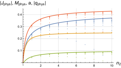
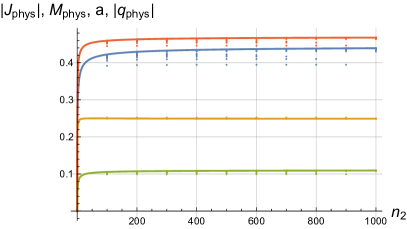
Figure 6.1: Plots of $|J_{\textrm{phys}}|$ (lowest curve), $M_{\textrm{phys}}$ (next to lowest on the left plot), $a$ (next to highest curve), and ${|{q}_{\textrm{phys}}|}$ (highest curve) as functions of a continuous variable $n_{2}\in[0,10]$ (left plot) and $n_{2}\in[0,1000]$ (right plot). The dots correspond to the values obtained for the solutions with the given values of $n_{2}$ and with $n_{1}$ increasing in logarithmic steps to $10000$ (left plot) and $100000$ (right plot).

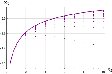
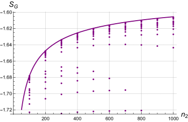
Figure 6.2: Plots of the gravitational contribution $S_{G}=-\Lambda V/(8\pi)$, scaled to $\Lambda=3$, to the Euclidean action $S$ as function of a continuous variable $n_{2}\in[0,10]$ (left plot) and $n_{2}\in[0,1000]$ (right plot). The dots correspond to the values obtained for the solutions with the given values of $n_{2}$ and with $n_{1}$ increasing in logarithmic steps to $10000$ (left plot) and $100000$ (right plot).

This leads to simple relations between various quantities for $n_{1}$ and $n_{2}$ large, as follows: for large $n_{2}$ we have the approximate relations

$$\sqrt{\frac{1}{n_{2}}} \approx \frac{5}{2}\sqrt{\frac{5}{2}}\left(\frac{1}{\sqrt{5}}-a\right)\approx\frac{25}{4}\sqrt{\frac{5}{2}}\left(\frac{4}{5\sqrt{5}}-M\right)\approx\frac{5}{2}\sqrt{\frac{5}{2}}\left(\frac{1}{\sqrt{5}}-{p^{2}_{\textrm{eff}}}\right)\approx\frac{2\sqrt{2}}{\pi}\left(-\frac{\pi}{2}-S_{G}\right)$$ (6.21)

$$\approx 27\sqrt{\frac{5}{2}}\left(M_{\textrm{phys}}-\frac{\sqrt{5}}{9}\right)\approx\frac{27}{\sqrt{2}}\left(\frac{1}{9}-|J_{\textrm{phys}}|\right)\approx 9\left(-\frac{\sqrt{3}}{2}-{|{q}_{\textrm{phys}}|}{}\right)\,.$$

From this one obtains various approximately affine relations between the quantities above for $1\ll n_{1}\ll n_{2}$, e.g.

$$|J_{\textrm{phys}}| \approx -\sqrt{5}M_{\textrm{phys}}+\frac{2}{3}\,,$$ (6.22)

$${|{q}_{\textrm{phys}}|} \approx -\frac{9}{3}M_{\textrm{phys}}+\frac{\sqrt{2}-\sqrt{5}}{3}\,,$$ (6.23)

$$S_{G} \approx -\frac{\sqrt{5}\pi}{4}M_{\textrm{phys}}-\frac{13}{36}\pi\,.$$ (6.24)

One can similarly make a second-order approximation in $1/n$, by expanding the quantities of interest up to $o(n^{-1})$ and eliminating $n$ from the equations. As an example, near the maximum value of $|q_{\textrm{phys}}|$ we obtain the relation

$$M_{\textrm{phys}}\approx\frac{3402\sqrt{2}|q_{\textrm{phys}}|+394\sqrt{3}\sqrt{5-7\sqrt{2}|q_{\textrm{phys}}|}-1437}{2205\sqrt{5}}\,.$$ (6.25)

The exact solution and the curve resulting from the second order approximation in $1/n$ can be seen in Figure 6.3.

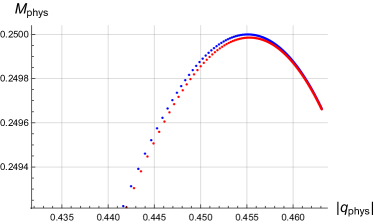
Figure 6.3: Correlation plot in the $(|q_{\textrm{phys}}|,M_{\textrm{phys}})$ plane in the limit $n_{1}\to\infty$. The red points lie on the curve (6.25), the blue dots arise from the exact solutions (6.13) and (6.15).

In Figure 6.4 we plot the dependence on the continuous variable $n_{2}$, in the $n_{1}\to\infty$ limit, of the area of the cross section of the horizon $A_{+}$ and the surface gravity $\kappa_{+}$ in the partner Lorentzian solutions.

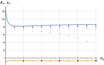
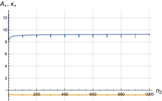
Figure 6.4: Plots of $A_{+}$(blue line) and $\kappa_{+}$(orange line) as functions of a continuous variable $n_{2}\in[0,10]$ (left plot) and $n_{2}\in[0,1000]$ (right plot). The dots correspond to the values obtained for the solutions with the given values of $n_{2}$ and with $n_{1}$ increasing in logarithmic steps to $10000$ (left plot) and $100000$ (right plot).

In Appendix D the reader will find a translation of some of the numerical values above to SI units.

7 Dirac strings

Similarly to [DuffMadore], the existence of charged spinor fields on the Euclidean manifold leads to further constraints on the parameters of the solution. Indeed, comparing (3.18) with (3.20) shows that the transition from a gauge potential which is regular near $\{\cos(\theta)=1\,,\ r=r_{i}\}$ to a gauge potential which is regular near $\{\cos(\theta)=-1\,,\ r=r_{i}\}$ requires a gauge transformation

$$A\mapsto A+\frac{2p}{\Xi}(\mathrm{d}\varphi-\frac{a}{a^{2}-r_{i}^{2}}\mathrm{d}t)\,.$$

If a Dirac field $\psi$ carries a charge $q_{0}$, such a gauge transformation induces a transformation

$$\psi\mapsto\exp\left(\frac{2iq_{0}p}{\hbar\Xi}\left(\varphi-\frac{a}{a^{2}-r_{i}^{2}}t\right)\right)\psi\,.$$

Recall that $\varphi$ is $2\pi/k$-periodic, with $k=1$ except in the Page limit where $k=2$ can arise and which needs to be analysed separately in any case, see Section LABEL:ss22I16.1 below. Thus in the remainder of this section we assume that $\varphi$ is $2\pi$ periodic. The requirement of single-valuedness of $\psi$ results in the condition

$$\frac{2q_{0}p}{\hbar\Xi}=:\hat{n}_{1}\in\mathbb{Z}\,.$$ (7.1)

Next, (3.18) and (3.21) show that the gauge potentials

$$A+\frac{p}{\Xi}(\mathrm{d}\varphi-\frac{a}{a^{2}-r_{i}^{2}}\mathrm{d}t)-\frac{er_{i}}{\Xi(a^{2}-r_{i}^{2})}\mathrm{d}t\,,\quad i=1,2,$$ (7.2)

are regular near $r=r_{i}$ and $\theta=0$. Passing from one to the other requires a gauge transformation

$$A\mapsto A+\left(\frac{pa+er_{2}}{\Xi(a^{2}-r_{2}^{2})}-\frac{pa+er_{1}}{\Xi(a^{2}-r_{1}^{2})}\right)\mathrm{d}t\,.$$

Keeping in mind that $t$ has period $2\pi\omega$, the associated transformation of the spinor field $\psi$ leads to the further condition

$$\underbrace{\frac{q_{0}}{\hbar\Xi}\bigg{(}p}_{\hat{n}_{1}/2}\big{(}\underbrace{\frac{a\omega}{r_{1}^{2}-a^{2}}}_{n_{1}}-\underbrace{\frac{a\omega}{r_{2}^{2}-a^{2}}}_{n_{2}}\big{)}+e\omega\big{(}\frac{r_{1}}{r_{1}^{2}-a^{2}}-\frac{r_{2}}{r_{2}^{2}-a^{2}}\big{)}\bigg{)}\in\mathbb{Z}^{*}\,.$$ (7.3)

A similar analysis near $\theta=\pi$ leads to the further condition

$$\underbrace{\frac{q_{0}}{\hbar\Xi}\bigg{(}p}_{\hat{n}_{1}/2}\big{(}\underbrace{\frac{a\omega}{r_{1}^{2}-a^{2}}}_{n_{1}}-\underbrace{\frac{a\omega}{r_{2}^{2}-a^{2}}}_{n_{2}}\big{)}-e\omega\big{(}\frac{r_{1}}{r_{1}^{2}-a^{2}}-\frac{r_{2}}{r_{2}^{2}-a^{2}}\big{)}\bigg{)}\in\mathbb{Z}^{*}\,.$$ (7.4)

We conclude that we must have

$$\frac{\hat{n}_{1}({n_{1}}-{n_{2}})}{2}\in\mathbb{N}^{*}\,,$$ (7.5)

and that there exists $\hat{n}_{2}\in\mathbb{N}^{*}$ so that

$$e\omega\left(\frac{r_{1}}{r_{1}^{2}-a^{2}}-\frac{r_{2}}{r_{2}^{2}-a^{2}}\right)=\hat{n}_{2}\,.$$ (7.6)

Eliminating $q_{0}$ between (7.1) and (7.3) imposes a quantised relation between $p$ and $e$:

$$p=\underbrace{\frac{\omega}{2}\left(\frac{r_{1}}{r_{1}^{2}-a^{2}}-\frac{r_{2}}{r_{2}^{2}-a^{2}}\right)}_{=:\sigma}\times\frac{\hat{n}_{1}}{\hat{n}_{2}}\times e\,.$$ (7.7)

Recall that given a set $(M,a,{p^{2}_{\textrm{eff}}})$, parameterised by two integers $(n_{1},n_{2})$ with $n_{1}<n_{2}$ and arising from a smooth compact Riemannian solution, we have so far been associating to it a Lorentzian partner solution with the same values of $M$ and $a$, with $p^{2}={p^{2}_{\textrm{eff}}}$ and with $e=0$. However, if one adds the requirement of well-defined charges spinor fields to the picture, instead of choosing $e=0$ on the Lorentzian side one might wish to request that (7.7) holds. This adds two further quantum numbers $(\hat{n}_{1},\hat{n}_{2})$ to the picture. Taking into account the inequality ${p^{2}_{\textrm{eff}}}=p^{2}-e^{2}>0$ one is led to the condition

$$\sigma\frac{\hat{n}_{1}}{\hat{n}_{2}}>1\,.$$ (7.8)

Given a pair $(\hat{n}_{1},\hat{n}_{2})$ such that (7.8) holds (note that this can always be achieved by choosing $\hat{n}_{1}$ large enough), we can determine $|q_{0}|$, $|e|$ and $|p|$ from (7.1)-(7.7):

$$\displaystyle|e|=\sqrt{\frac{{p^{2}_{\textrm{eff}}}}{(\sigma\frac{\hat{n}_{1}}{\hat{n}_{2}})^{2}-1}}\,,\quad|p|={\sigma\frac{\hat{n}_{1}}{\hat{n}_{2}}}\sqrt{\frac{{p^{2}_{\textrm{eff}}}}{(\sigma\frac{\hat{n}_{1}}{\hat{n}_{2}})^{2}-1}}\,,\quad|q_{0}|=\frac{\hbar\Xi}{2}\sqrt{\frac{\sigma^{2}\hat{n}_{1}^{2}-\hat{n}_{2}^{2}}{{p^{2}_{\textrm{eff}}}}}\,.$$

In this way we are led to a discrete family of solutions parameterised by four integers $(n_{1},n_{2},\hat{n}_{1},\hat{n}_{2})$ subject to the constraints (7.5) and (7.8).

It holds that ${p^{2}_{\textrm{eff}}}<p^{2}\to_{(\hat{n}_{1}/\hat{n}_{2})\to\infty}{{p^{2}_{\textrm{eff}}}}$, $e\to_{(\hat{n}_{1}/\hat{n}_{2})\to\infty}0$, and thus ${p^{2}_{\textrm{eff}}}<p^{2}+e^{2}\to_{(\hat{n}_{1}/\hat{n}_{2})\to\infty}{{p^{2}_{\textrm{eff}}}}$.

The global structure of the resulting Lorentzian partners is the same as in the case $e=0$, see Figure B.1.

Appendix A A typical solution

We rescale the metric so that $\lambda=1$. We choose $n_{1}=10$, $n_{2}=9$. With this choice the system (5.3-5.7) takes the explicit form

$$-a^{2}+{p^{2}_{\textrm{eff}}}-2Mr_{1}+r_{1}^{2}+a^{2}r_{1}^{2}-r_{1}^{4} = 0\,,$$

$$-2a+2a^{3}-20M+20r_{1}+20a^{2}r_{1}-40r_{1}^{3} = 0\,,$$

$$-2a+2a^{3}+18M-18r_{2}-18a^{2}r_{2}+36r_{2}^{3} = 0\,,$$

$$10(r_{1}^{2}-a^{2})-9(r_{2}^{2}-a^{2}) = 0\,,$$ (A.1)

as well as an equation for $r_{2}$ identical to the first equation above. The Buchberger algorithm for finding a Gröbner basis for Eq.(A.1), as implemented in Mathematica, yields the following system

$$141447860388864000000({p^{2}_{\textrm{eff}}})^{2}-2530102285619187840000({p^{2}_{\textrm{eff}}})^{3}+6902836371659336516100({p^{2}_{\textrm{eff}}})^{4}$$

$$-7443462023036715884580({p^{2}_{\textrm{eff}}})^{5}+3324944139689702617201({p^{2}_{\textrm{eff}}})^{6} = 0\,,$$

$$269121969463191443505728626849880910201000({p^{2}_{\textrm{eff}}})^{2}+5123491133454465890342571180870383758599000a^{2}({p^{2}_{\textrm{eff}}})^{2}$$

$$-4306620505226193997812468562360852027723500({p^{2}_{\textrm{eff}}})^{3}+661016788713267074222610725116146960042870({p^{2}_{\textrm{eff}}})^{4}$$

$$-1418820167927814403912453122762613275222257({p^{2}_{\textrm{eff}}})^{5} = 0\,,$$

$$1840946142733449839332390348051522429788563882649600000M({p^{2}_{\textrm{eff}}})$$

$$-140403030498229867043777134104718536116027658797039040000a({p^{2}_{\textrm{eff}}})^{2}$$

$$+425794621585557982844978758649217892223137640430823652700a({p^{2}_{\textrm{eff}}})^{3}$$

$$-476718734408676529956326149018521215355879124052827578300a({p^{2}_{\textrm{eff}}})^{4}$$

$$+216318197798255246294998226248424687617679013902862944743a({p^{2}_{\textrm{eff}}})^{5} = 0\,,$$

$$10604338062917514381295873956265388153861661532099121130946560000000a^{3}$$

$$-10604338062917514381295873956265388153861661532099121130946560000000a^{5}$$

$$+1767389677152919063549312326044231358976943588683186855157760000000a({p^{2}_{\textrm{eff}}})$$

$$-588227304146277718291223364304260174172128286418763128059980799680000a({p^{2}_{\textrm{eff}}})^{2}$$

$$+1755642879359412179543337165217487045071628171531789605489627506273900a({p^{2}_{\textrm{eff}}})^{3}$$

$$-1954502602810413009680346541725810677017518746391376355441883692255820a({p^{2}_{\textrm{eff}}})^{4}$$

$$+893243009923318159877420930128536388883746991239505692176977591346539a({p^{2}_{\textrm{eff}}})^{5}$$

$$+3534779354305838127098624652088462717953887177366373710315520000000({p^{2}_{\textrm{eff}}})r_{2} = 0\,,$$

together with an identical equation for $r_{1}$.

The structure of the equations is typical in the following sense: Since Mathematica does not manage to find a Gröbner basis when $n_{1}$ and $n_{2}$ are left as general parameters, our procedure is to provide the values of $n_{1}$ and $n_{2}$ and then seek the basis. All the resulting polynomials that we have inspected have then a structure identical to the one above.

It can be seen that solving the system (LABEL:19V15.5) in the manner described above requires only solving polynomial equations in a single variable of at most forth order, and so explicit analytic expressions can be given. However, the expressions obtained, especially for $r_{1}$ and $r_{2}$, become very unwieldy. Therefore, instead of the full analytic expressions, we give only the first five nontrivial digits after the decimal point of the parameters for the solution of (A.1) that fulfills the constraints:

$$r_{1}=0.48613\,,~{}~{}r_{2}=0.51203\,,~{}~{}M=0.25211\,,~{}~{}a=0.060481\,,~{}~{}{p^{2}_{\textrm{eff}}}=0.067439\,.$$ (A.3)

Appendix B Physical quantities

B.1 Euclidean case

The “surface gravity” of the zeros of the $\partial_{t}$-Killing vector, located at $r_{1}$ and $r_{2}$, reads

$$\kappa:=\frac{1}{2\Xi(r_{i}^{2}-a^{2})}\Delta_{r}^{\prime}|_{r={r_{1}}}=-\frac{1}{2\Xi(r_{i}^{2}-a^{2})}\Delta_{r}^{\prime}|_{r={r_{2}}}\,.$$ (B.1)

Since $\partial_{\varphi}$ and $\partial_{t}$ are Killing fields and

$$(t,r,\theta,\varphi)\in[0,\frac{2\pi}{\kappa})\times[r_{1},r_{2})\times[0,\pi)\times[0,2\pi)\,,$$

we obtain the following formula for the areas of the zero-set of $\partial_{t}$, located at $r_{1}$ and $r_{2}$,

$$A_{i} = 2\pi\int_{0}^{\pi}\sqrt{g_{\varphi\varphi}g_{\theta\theta}}|_{r={r_{i}}}\,d\theta=\pi\int_{0}^{\pi}\frac{\left(r_{i}^{2}-a^{2}\right)\sin(\theta)}{\Xi}\,d\theta\,$$ (B.2)

$$= \frac{4\pi\left(r_{i}^{2}-a^{2}\right)}{\Xi}\,$$

and for the volume of the manifold

$$V = 2\pi\frac{2\pi}{\kappa}\int_{r_{1}}^{r_{2}}\int_{0}^{\pi}\sqrt{g}\,d\theta dr=\frac{4\pi^{2}}{\kappa}\int_{r_{1}}^{r_{2}}\int_{0}^{\pi}\frac{\Sigma\sin(\theta)}{\Xi^{2}}\,d\theta dr\,$$ (B.3)

$$= \frac{8\pi^{2}}{{3\kappa\Xi^{2}}}\left[\left(r_{2}^{3}-r_{1}^{3}\right)-a^{2}(r_{2}-r_{1})\right]\,.$$

The action of the Einstein-Maxwell system is given by

$$S = -\frac{1}{16\pi}\int(R-2\Lambda-F^{2})\sqrt{g}\,d^{4}x\,$$ (B.4)

$$= \underbrace{-\frac{1}{16\pi}\int(R-2\Lambda)\sqrt{g}\,d^{4}x}_{:=S_{G}}\,+\underbrace{\frac{1}{16\pi}\int F^{2}\sqrt{g}\,d^{4}x}_{:=S_{\mbox{\rm\tiny EM}}}\,.$$

Let $S_{G}$ be the gravitational action, we have

$$S_{G} = -\frac{1}{16\pi}\int(R-2\Lambda)\sqrt{g}\,d^{4}x\,$$ (B.5)

$$= -\frac{\Lambda}{8\pi}V\,$$

$$= -\Lambda\frac{\pi}{3\kappa\Xi^{2}}\left[\left(r_{2}^{3}-r_{1}^{3}\right)-a^{2}(r_{2}-r_{1})\right]\,.$$

A Mathematica calculation gives

$$F^{2}:=g^{\alpha\beta}g^{\mu\nu}F_{\alpha\mu}F_{\beta\nu}=\frac{(e-p)^{2}}{(a\cos(\theta)+r)^{4}}+\frac{(e+p)^{2}}{(r-a\cos(\theta))^{4}}\,,$$ (B.6)

leading to

$$S_{\mbox{\rm\scriptsize EM}} = \frac{1}{16\pi}\int F^{2}\sqrt{g}\,d^{4}x\,$$ (B.7)

$$= \frac{1}{16\pi}\frac{4\pi^{2}}{\kappa}\int_{r_{1}}^{r_{2}}\int_{0}^{\pi}\,F^{2}\sqrt{g}d\theta dr\,$$

$$= \frac{\pi(p^{2}+e^{2})}{\kappa\Xi^{2}}\left(\frac{r_{1}}{r_{1}^{2}-a^{2}}-\frac{r_{2}}{r_{2}^{2}-a^{2}}\right)\,\,.$$

Together this yields

$$S=\frac{\pi}{\kappa\Xi^{2}}\left\{-\frac{\Lambda}{3}\left[\left(r_{2}^{3}-r_{1}^{3}\right)-a^{2}(r_{2}-r_{1})\right]+(e^{2}+p^{2})\left(\frac{r_{1}}{r_{1}^{2}-a^{2}}-\frac{r_{2}}{r_{2}^{2}-a^{2}}\right)\right\}\,.$$ (B.8)

The minimum of the action is attained at $(n_{1},n_{2})=(2,1)$, and equals $S_{\min{}}\approx-2.357$. Since $r_{1}\to_{n_{1}\to\infty}a$ and ${p^{2}_{\textrm{eff}}}\to_{n_{1}\to\infty}0.32$ (see (6.11)), the action is unbounded from above. It follows from the analysis in Section 6 that $S_{G}$ is bounded from above by $-\pi/2$, so only the Maxwell action grows without bound. Now, if $r_{2}$ is close to $r_{1}$, then the Maxwell action is very small. One expects this to be true when both $n_{1}$ and $n_{2}$ are very large. This suggests very strongly that the set of pairs $(n_{1},n_{2})$, for which the Maxwell action $S_{\mbox{\rm\scriptsize EM}}$ is very small compared to the gravitational one, is unbounded. Numerics shows that this is indeed the case for all large numbers $n_{1}$ that we have looked at.

In particular solutions with very large values of $n_{1}-n_{2}$ are strongly suppressed when path-integral arguments are invoked.

B.2 Lorentzian case

In this section we consider the Lorentzian solutions with $e=0$ and with the value of $a$, $M$ and ${p^{2}_{\textrm{eff}}}$ arising from a smooth compact Euclidean solution with $e=0$. To avoid ambiguities, we write

$$\Delta_{\mathrm{Lor}}:=(r^{2}+a^{2})(1-\lambda r^{2})-2Mr+p^{2}+e^{2}\,\ \textrm{ and }\ \Xi_{{{\mathrm{Lor}}}}:=1+\lambda a^{2}\,.$$ (B.9)

In all solutions that we have found the function $\Delta_{{{\mathrm{Lor}}}}$ has precisely two real first-order zeros, with exactly one positive, denoted by $r_{+}$. The associated horizon is usually referred to as the cosmological horizon. The global structure of the Lorentzian solution is shown in Figure B.1.

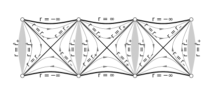
Figure B.1: A projection diagram for the Kerr-Newman - de Sitter metrics with exactly two distinct real first-order zeros of $\Delta_{r}$, $r_{-}<0<r_{+}$, from [COS]. Outside of the shaded regions, which contain the singular rings and the time-machines with boundaries at $\hat{r}_{\pm}$, the diagram represents accurately (within the limitations of a two-dimensional projection) the global structure of the space-time. Here $r_{-}$ and $r_{+}$ indicate the radii of the Lorentzian horizons, not to be confused with the Euclidean rotation axes from the body of the paper.

As already pointed-out, there is an ambiguity in the definition of total mass of the associated Lorentzian space-time. In a Hamiltonian approach this ambiguity is related to the choice of the Killing vector field for which we calculate the Hamiltonian [CJKKerrdS]. In any case, the physical mass $M_{\textrm{phys}}$ and the angular momentum $J_{\textrm{phys}}$ are usually calculated using the formulae

$$M_{\textrm{phys}}=\frac{M}{\Xi_{{{\mathrm{Lor}}}}^{2}}\,,\quad J_{\textrm{phys}}=\frac{aM}{\Xi_{{{\mathrm{Lor}}}}^{2}}\,.$$ (B.10)

(The above mass of the Lorentzian solution is obtained by calculating the Hamiltonian associated with the Killing vector field $\Xi_{{{\mathrm{Lor}}}}\partial_{t}+3^{-1}\Lambda a\partial_{\varphi}$, while the total angular momentum is the Hamiltonian associated with $\partial_{\varphi}$.)

The area of the cross-section of the horizon located at $r_{+}$ is given by

$$A_{+}=\frac{4\pi\left(r_{+}^{2}+a^{2}\right)}{\Xi_{{{\mathrm{Lor}}}}}\,,$$ (B.11)

and is usually interpreted as the entropy of the cosmological horizon [GibbonsHawkingCEH]. The surface gravity of the horizon $r=r_{+}$ associated with the Killing vector $X:=\partial_{t}+\Omega\partial_{\varphi}$, where $\Omega$ is chosen so that $X$ is tangent to the generators of the horizon, is

$$\kappa_{+}=\frac{1}{2\Xi_{{{\mathrm{Lor}}}}(r_{+}^{2}+a^{2})}\Delta_{{{\mathrm{Lor}}}}^{\prime}|_{r={r_{+}}}\,.$$ (B.12)

Appendix C A sample

We list in Table C.1 the defining parameters of all solutions for $\lambda=1,\;\zeta=-1\,,n_{1},n_{2}\in\{-10,10\}\,,n_{1}>n_{2}$, fulfilling the constraints, as well as some associated physical quantities. The constraints $a<r_{1}<r_{2}$ and $a^{2}<1$ are clearly seen to be fulfilled. The physical quantities $M_{\textrm{phys}}$, $|J_{\textrm{phys}}|$, ${|{q}_{\textrm{phys}}|}$ are defined in (B.10), while ${S}$ denotes the Euclidean action of the solutions.

$$\tiny\begin{array}[]{ccccccccccccc}n_{1}&n_{2}&n_{1}-n_{2}&\text{a}&r_{1}&r_{2}&\text{M}&p^{2}_{\textrm{eff}}{}&M_{\textrm{phys}}&|J_{\textrm{phys}}|&{|{q}_{\textrm{phys}}|}&S_{G}&S\\ 2&1&1&0.05720&0.4147&0.5837&0.2449&0.06344&0.2433&0.01392&0.2511&-2.368&-2.357\\ 3&1&2&0.09837&0.3698&0.6253&0.2398&0.06764&0.2352&0.02314&0.2576&-2.377&-2.335\\ 3&2&1&0.05939&0.4494&0.5488&0.2497&0.06610&0.2480&0.01473&0.2562&-2.353&-2.340\\ 4&1&3&0.1264&0.3426&0.6493&0.2366&0.07260&0.2292&0.02898&0.2652&-2.380&-2.291\\ 4&2&2&0.1063&0.4159&0.5785&0.2504&0.07462&0.2449&0.02604&0.2701&-2.341&-2.290\\ 4&3&1&0.05997&0.4638&0.5344&0.2510&0.06681&0.2492&0.01494&0.2576&-2.349&-2.336\\ 5&1&4&0.1460&0.3247&0.6646&0.2346&0.07709&0.2249&0.03284&0.2718&-2.380&-2.233\\ 5&2&3&0.1403&0.3930&0.5971&0.2518&0.08399&0.2422&0.03398&0.2842&-2.326&-2.211\\ 5&3&2&0.1088&0.4370&0.5571&0.2538&0.07688&0.2479&0.02698&0.2740&-2.330&-2.276\\ 5&4&1&0.06020&0.4717&0.5265&0.2515&0.06710&0.2497&0.01503&0.2581&-2.347&-2.334\\ 6&1&5&0.1602&0.3120&0.6751&0.2333&0.08086&0.2217&0.03553&0.2772&-2.380&-2.165\\ 6&2&4&0.1648&0.3768&0.6096&0.2533&0.09238&0.2401&0.03957&0.2959&-2.312&-2.110\\ 6&3&3&0.1452&0.4173&0.5721&0.2571&0.08814&0.2466&0.03580&0.2908&-2.308&-2.182\\ 6&4&2&0.1100&0.4492&0.5447&0.2552&0.07789&0.2492&0.02740&0.2758&-2.325&-2.270\\ 6&5&1&0.06032&0.4767&0.5215&0.2518&0.06724&0.2499&0.01508&0.2584&-2.346&-2.333\\ \end{array}$$ (C.17)

Table C.1: Some selected solutions with the most relevant physical parameters in dimensionless units

Appendix D SI units

Recall that $\lambda:=\Lambda/3$. The replacements

$$r\mapsto\sqrt{\frac{1}{\lambda}}\times r\,,\quad M\mapsto\sqrt{\frac{1}{\lambda}}\times M\,,\quad a\mapsto\sqrt{\frac{1}{\lambda}}\times a\,,\quad e\mapsto\sqrt{\frac{1}{\lambda}}\times e\,,$$ (D.1)

yield

$$\Delta_{r}\mapsto\frac{1}{\lambda}\Big{(}\underbrace{(r^{2}+a^{2})\left(1-r^{2}\right)-2Mr+p^{2}_{\textrm{eff}}{}}_{:=\Delta^{\lambda=1}_{r}}\Big{)}\,,\quad\Delta^{\prime}_{r}\mapsto\frac{1}{\sqrt{\lambda}}\Delta^{\prime\lambda=1}_{r}\,,\quad\Xi\mapsto\underbrace{1-a^{2}}_{:=\Xi^{\lambda=1}}\,.$$

It is easy to check that if

$$\Big{(}r_{1}^{\lambda=1},r_{2}^{\lambda=1},M^{\lambda=1},a^{\lambda=1},(p^{2}_{\textrm{eff}}{})^{\lambda=1}\Big{)}$$

is a solution of the system Eq.(5.3-5.7) for $\lambda=1$, then

$$r_{1} = \sqrt{\frac{1}{\lambda}}\times r_{1}^{\lambda=1}\,,\quad r_{2}=\sqrt{\frac{1}{\lambda}}\times r_{2}^{\lambda=1}\,,\quad M=\sqrt{\frac{1}{\lambda}}\times M^{\lambda=1}\,,$$

$$a = \sqrt{\frac{1}{\lambda}}\times a^{\lambda=1}\,,\quad p^{2}_{\textrm{eff}}{}=\frac{1}{\lambda}\times(p^{2}_{\textrm{eff}}{})^{\lambda=1}\,,$$ (D.3)

provides a solution of this system with an arbitrary value $\lambda$.

In SI-units we have

$$M_{\textrm{phys}}^{SI}=\frac{c^{2}}{G}\times M_{\textrm{phys}}\,,\quad{|{q}_{\textrm{phys}}|}^{SI}=\sqrt{\frac{4\pi\epsilon_{0}c^{4}}{G}}\times{|{q}_{\textrm{phys}}|}\,,$$ (D.4)

where $G$ is the gravitational constant, $c$ the speed of light and $\epsilon_{0}$ the electric constant. Then the physical angular momentum in SI-units can be computed as

$$J_{\textrm{phys}}^{SI} = a\times c\times M_{\textrm{phys}}^{SI}\;.$$ (D.5)

Putting all this together we obtain

$$M_{\textrm{phys}}^{SI} = \frac{c^{2}}{G}\times\frac{1}{\Xi_{{{\mathrm{Lor}}}}^{2}}\times\sqrt{\frac{1}{\lambda}}\times M^{\lambda=1}\,,$$ (D.6)

$$a^{SI} = \sqrt{\frac{1}{\lambda}}\times a^{\lambda=1}\,,$$ (D.7)

$${|{q}_{\textrm{phys}}|}{}^{SI} = \sqrt{\frac{4\pi\epsilon_{0}c^{4}}{G}\times\frac{1}{\lambda}\times\frac{1}{\Xi_{{{\mathrm{Lor}}}}^{2}}\times(p^{2}_{\textrm{eff}}{})^{\lambda=1}}\,,$$ (D.8)

$$J_{\textrm{phys}}^{SI} = c\times a^{SI}\times M_{\textrm{phys}}^{SI}\;.$$ (D.9)

Since $\Xi_{\mathrm{{Lor}}}$ and $\Delta_{\mathrm{{Lor}}}$ are invariant under rescaling, it follows

$$A_{+}^{SI} = \frac{1}{\lambda}A_{+}^{\lambda=1}\,,$$ (D.10)

$$\kappa_{+}^{SI} = c^{2}\sqrt{\lambda}\kappa_{+}^{\lambda=1}\,.$$ (D.11)

The black hole temperature in SI-units $T^{SI}$ reads

$$T_{kg^{-1}} = \frac{1}{2\pi}\frac{G}{c^{2}}\sqrt{\lambda}\times\kappa_{+}^{\lambda=1}\,,$$ (D.12)

$$T^{SI} = \frac{c^{3}\hbar}{k\,G}\times T_{kg^{-1}}\,,$$ (D.13)

where $\hbar=1.054\times 10^{-34}\,Js$ and $k=1.38\times 10^{-23}JK^{-1}$ are the reduced Planck’s constant and the Boltzmann constant respectively. Table D.1 lists some values of $M_{\textrm{phys}}$ in units of the mass of Milky Way, taken to be $10^{12}M_{\odot}$,

$$M_{\textrm{phys}}=M_{\textrm{astro}}\times 10^{12}M_{\odot}\sqrt{\frac{\Lambda}{\Lambda_{0}}}\,,$$

where $M_{\odot}$ is the mass of the sun and

$$\Lambda_{0}=3H_{0}^{2}\Omega_{\Lambda}=1.11\times 10^{-52}\;m^{-2}$$

is the value of the cosmological constant as resulting from the Planck observations [Planck16.2013] (compare [Planck13, Supernova2004, Komatsu:2010fb]). We moreover use $G=6.67\times 10^{-11}\;\frac{m^{3}}{kgs^{2}}$, $c=299\times 10^{8}\;\frac{m}{s}$, and $\epsilon_{0}=8.85\times\;10^{-12}m^{-3}kg^{-1}s^{4}A^{2}$, $M_{{}_{\odot}}=1.99\times 10^{30}\;kg$.

$M_{\textrm{phys}}/10^{10}M_{\textrm{Milky Way}}$	type
$2.27$	minimum
$2.84$	maximum
$2.71$	at minimal charge
$2.77$	at maximal charge

Table D.1: Some cosmological values of $M_{\textrm{phys}}$, in Milky Way mass units.

Another set of amusing questions is, which values of $\Lambda$ are required to obtain the charge $e^{-}$ of an electron as minimal value for the physical charge ${|{q}_{\textrm{phys}}|}{}^{SI}=e^{-}$, or the mass of an electron $M_{\mathrm{e}}$, or of a proton $M_{\mathrm{p}}$, as minimal value of the physical mass:

$$e^{-}=1.60\times 10^{-19}C\,,\quad M_{\mathrm{e}}=9.11\times 10^{-31}kg\,,\quad M_{\mathrm{p}}=1.67\times 10^{-27}kg\,.$$

The results are given in Table D.2.

minimal physical mass /charge	$\Lambda$ / $m^{-2}$	$\Lambda$ / $\Lambda_{0}$
$e^{-}$	$9.92\times 10^{70}$	$8.94\times 10^{122}$
$M_{\mathrm{e}}$	$2.72\times 10^{113}$	$2.45\times 10^{165}$
$M_{\mathrm{p}}$	$8.06\times 10^{106}$	$7.26\times 10^{158}$

Table D.2: Values of $\Lambda$ required to obtain $e^{-}$ as minimal physical charge and $M_{\mathrm{e}}$/ $M_{\mathrm{p}}$ as minimal physical mass. $\Lambda_{0}$ is the current estimate of the value of the cosmological constant.

Appendix E Lorentzian partner solutions

Consider a set of parameters $n_{1}$, $n_{2}$, $M$, $a$, and $p^{2}_{\textrm{eff}}{}$ that solve, together with the positive zeros of $\Delta_{r}$, the system (5.3-5.7) and fulfill the constraints. For this set of parameters we calculate the zeros of the Lorentzian partner $\Delta_{{{\mathrm{Lor}}}}$ given by (B.9) of the Euclidean function $\Delta_{r}$. As already mentioned, for all $(n_{1},n_{2})$ that we have investigated the function $\Delta_{{{\mathrm{Lor}}}}$ has only two real first-order zeros, with exactly one positive zero $r_{+}$.

E.1 Geometric units

In Table E.1 we list the values of $r_{+}$, the surface gravity (“temperature”) and the area (“entropy”) of the horizon.

$$\tiny\begin{array}[]{cccccc}n_{1}&n_{2}&n_{1}-n_{2}&r_{+}&\kappa_{+}&A_{+}\\ 2&1&1&0.612&-0.246&4.730\\ 3&1&2&0.667&-0.377&5.663\\ 3&2&1&0.594&-0.216&4.467\\ 4&1&3&0.699&-0.452&6.239\\ 4&2&2&0.649&-0.355&5.368\\ 4&3&1&0.589&-0.208&4.394\\ 5&1&4&0.719&-0.498&6.617\\ 5&2&3&0.682&-0.439&5.967\\ 5&3&2&0.643&-0.349&5.282\\ 5&4&1&0.587&-0.204&4.364\\ 6&1&5&0.732&-0.529&6.880\\ 6&2&4&0.703&-0.493&6.376\\ 6&3&3&0.676&-0.438&5.890\\ 6&4&2&0.641&-0.346&5.244\\ 6&5&1&0.586&-0.203&4.349\\ \end{array}$$ (E.17)

Table E.1: The surface gravity and area for some selected solutions, with $\Lambda=3$.

E.2 SI units, $\Lambda=1.11\times 10^{-52}\;m^{-2}$

With the formulae given in Appendix D we can calculate the interesting physical quantities in SI-units for the measured cosmological value $\Lambda_{0}$ of $\Lambda$ from the data for $\Lambda=3$. Using the Planck mission data $\Omega_{\Lambda}=0.6911$ and $H_{0}=67.74\,km/(s\,Mpc)$, (see [Planck13], p. 31, TT, TE, EE + lowP + lensing), the cosmological constant can be calculated to be

$$\Lambda_{0}c^{2}=3\,H_{0}^{2}\,\Omega_{\Lambda}=9.99\times 10^{-36}s^{-2}\Rightarrow\Lambda_{0}=1.11\times 10^{-52}\;m^{-2}\;$$

The reader will find some physical quantities of interest associated with our solutions in Tables E.2 and E.3.

$$\tiny\begin{array}[]{cccccccccc}n_{1}&n_{2}&n_{1}-n_{2}&r_{+}/10^{26}m&M_{phys}/10^{52}kg&|J_{phys}|/10^{86}kgm^{2}s^{-1}&|q_{phys}|/10^{42}C&|\kappa_{+}|/10^{-10}ms^{-2}&A_{+}/10^{53}m^{2}&T/10^{-30}K\\ 2&1&1&1.006&5.387&1.519&4.790&1.345&1.278&0.545\\ 3&1&2&1.097&5.207&2.524&4.914&2.062&1.530&0.836\\ 3&2&1&0.977&5.490&1.607&4.888&1.181&1.207&0.479\\ 4&1&3&1.149&5.074&3.162&5.060&2.470&1.686&1.001\\ 4&2&2&1.066&5.421&2.841&5.153&1.938&1.451&0.786\\ 4&3&1&0.969&5.517&1.631&4.914&1.136&1.188&0.461\\ 5&1&4&1.181&4.978&3.583&5.186&2.723&1.788&1.104\\ 5&2&3&1.120&5.362&3.708&5.422&2.401&1.613&0.974\\ 5&3&2&1.057&5.487&2.944&5.228&1.906&1.427&0.773\\ 5&4&1&0.966&5.528&1.640&4.924&1.117&1.179&0.453\\ 6&1&5&1.203&4.909&3.877&5.289&2.891&1.859&1.172\\ 6&2&4&1.156&5.316&4.318&5.645&2.696&1.723&1.093\\ 6&3&3&1.112&5.459&3.906&5.547&2.393&1.592&0.970\\ 6&4&2&1.053&5.517&2.990&5.261&1.893&1.417&0.768\\ 6&5&1&0.964&5.534&1.645&4.929&1.108&1.175&0.449\\ \end{array}$$ (E.34)

Table E.2: Some physical quantities in SI units for selected solutions

$$\tiny\begin{array}[]{cccccccccccccccc}n_{1}&2&3&3&4&4&4&5&5&5&5&6&6&6&6&6\\ n_{2}&1&1&2&1&2&3&1&2&3&4&1&2&3&4&5\\ \frac{M_{phys}}{M_{\odot}}/10^{22}&2.708&2.618&2.760&2.551&2.726&2.774&2.503&2.696&2.759&2.779&2.468&2.672&2.745&2.774&2.782\\ =\frac{M_{phys}}{M_{gal}}/10^{10}&&&&&&&&&&&&&&&\\ \end{array}$$ (E.39)

Table E.3: The physical mass in solar mass- and galaxy mass units for some selected solutions

To close this section, let us assume that the above universe consists of protons, neutrons, and hydrogen atoms. This means that for the range of values, as given above, we have $n_{\mbox{\scriptsize\rm items}}\approx M_{\textrm{phys}}/M_{\mbox{\scriptsize\rm proton}}\approx 2\times 10^{79}$ items. On the other hand $n_{\mbox{\scriptsize\rm protons}}=|q_{\textrm{phys}}|/e^{-}\approx 2\times 10^{61}$ particles are required to produce the required charge. As a consequence, every $10^{18}$-th item carries a charge.