Globular Cluster Systems in Brightest Cluster Galaxies. II: NGC 6166

Abstract

We present new deep photometry of the globular cluster system (GCS) around NGC 6166, the central supergiant galaxy in Abell 2199. HST data from the ACS and WFC3 cameras in $F475W,F814W$ are used to determine the spatial distribution of the GCS, its metallicity distribution function (MDF), and the dependence of the MDF on galactocentric radius and on GC luminosity. The MDF is extremely broad, with the classic red and blue subpopulations heavily overlapped, but a double-Gaussian model can still formally match the MDF closely. The spatial distribution follows a Sérsic-like profile detectably to a projected radius of at least $R_{gc}=250$ kpc. To that radius, the total number of clusters in the system is $N_{GC}=39000\pm 2000$, the global specific frequency is $S_{N}=11.2\pm 0.6$, and 57% of the total are blue, metal-poor clusters. The GCS may fade smoothly into the Intra-Cluster Medium of A2199; we see no clear transition from the core of the galaxy to the cD halo or the ICM. The radial distribution, projected ellipticity, and mean metallicity of the red (metal-richer) clusters match the halo light extremely well for $R_{gc}\gtrsim 15$ kpc, both of them varying as $\sigma_{MRGC}\sim\sigma_{light}\sim R^{-1.8}$. By comparison, the blue (metal-poor) GC component has a much shallower falloff $\sigma_{MPGC}\sim R^{-1.0}$ and a more nearly spherical distribution. This strong difference in their density distributions produces a net metallicity gradient in the GCS as a whole that is primarily generated by the population gradient. With NGC 6166 we appear to be penetrating into a regime of high enough galaxy mass and rich enough environment that the bimodal two-phase description of GC formation is no longer as clear or effective as it has been in smaller galaxies.

1. Introduction

Brightest Cluster Galaxies (BCGs) are the largest galaxies in the universe, and as such they are likely to have evolved from the most complex and extended hierarchical-merger trees during the most rapid stage of galaxy assembly. Their growth is still ongoing today as they accrete smaller galaxies within their host clusters.

BCGs also host the richest populations of globular clusters (GCs), a mark of exceptionally intense star formation under conditions of high gas density at high redshift. The nearest examples of these high-specific-frequency globular cluster systems (GCSs) include those within M87 in Virgo (Harris, 2009b), NGC 1399 in Fornax (Bassino et al., 2006), and NGC 3311 in Hydra (Wehner et al., 2008). These cases are, however, eclipsed by the still more luminous giants that can be found by searching further outward. A well known example is NGC 4874 in Coma (Peng et al., 2011), which may hold $\simeq 23000$ GCs of its own, and a still richer system may lie within Abell 1689 (Alamo-Martínez et al., 2013). Furthermore, a rich galaxy cluster may also contain an extended Intra-Cluster Medium (ICM) of stellar light and high-temperature X-ray gas, and the ICM itself can hold large numbers of intragalactic globular clusters (IGCs) that may even exceed the total in the central BCG (see Peng et al., 2011; Durrell et al., 2014). The IGCs may in turn be a combination of objects stripped from other galaxies in the cluster, and ones in the cD halo of the central BCG. In short, these systems offer a testing ground of unequalled richness for exploring GC systematics observationally.

Incorporating GCs fully into hierarchical galaxy formation models is difficult because spatial resolutions less than $\sim 1$ pc are needed to trace star cluster formation, while the galaxy as a whole needs a scale six orders of magnitude larger. But appropriately designed models have had some initial success at reproducing the observed GC mass distribution, and perhaps more challengingly, the metallicity distribution (e.g. Kravtsov & Gnedin, 2005; Muratov & Gnedin, 2010; Griffen et al., 2010; Tonini, 2013; Li & Gnedin, 2014). The existing models, though still quite preliminary, already hint that the GC metallicity distribution function (MDF) changes significantly with host galaxy mass even among large galaxies. The BCGs represent the relatively unexplored extreme upper limit of any such trends.

In Paper I (Harris et al., 2014), we introduced a new HST-based imaging survey of seven BCGs, aimed primarily at studying the GCSs in these biggest of all galaxies. Paper I contained a discussion of the luminosity and mass distribution function of their GC populations. In the current paper, we present more detailed results for the nearest of these seven systems, NGC 6166, including the GCS spatial distribution and total population, and the distribution of GCs by color and metallicity. Similar material for the remaining six galaxies will be presented in the next paper of our series.

For NGC 6166 we assume $d=130$ Mpc for $H_{0}=70$ km s^-1 Mpc^-1 along with a foreground reddening $E(F475W-F814W)=0.023$ at ($\ell=62.9^{o},b=43.7^{o}$). The adopted distance modulus is $(m-M)_{I}=35.60$ and the galaxy luminosity is $M_{V}^{T}=-23.7$ (Paper I).

2. Photometric Reductions

NGC 6166 is a classic cD galaxy with an extremely extended halo (Bender et al., 2015, hereafter B15) and is the central supergiant galaxy in Abell 2199. Early detections of its rich GCS with ground-based imaging were done by Pritchet & Harris (1990) from the Canada-France-Hawaii Telescope, Bridges et al. (1996) from the William Herschel Telescope, and Blakeslee et al. (1997) with the MDM Observatory. With ground-based imaging, however, only the brightest magnitude or two of the GC luminosity function and approximate mean color indices could be measured, yielding very uncertain estimates of the spatial extent or specific frequency of the system.

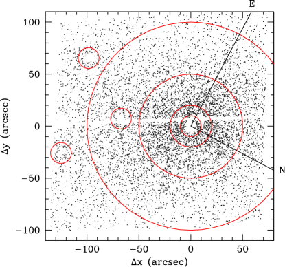
Figure 1.— Locations of the measured starlike objects ($x,y$ in arcseconds relative to the center of NGC 6166) for the brightest objects, $F814W<27.2$. The large concentric circles have radii of $20^{\prime\prime},50^{\prime\prime},100^{\prime\prime}$. The three smaller circles of radii $10^{\prime\prime}$ mark the three companion galaxies NGC 6166A, NGC 6166D, and PGC058261 (see text). The visible gap running across the middle of the frame is the gap between the two CCD detectors in the ACS/WFC. The fiducial directions towards North and East on the sky are marked; the +x-axis of the ACS camera is oriented $28^{o}$ E of N.

By contrast, the HST cameras are extremely well suited to imaging of GCSs in giant galaxies at distances of $\sim 100-200$ Mpc where the field sizes of either the ACS or WFC3 arrays correspond to linear diameters near 100 kpc, while the bright half of the GC luminosity function (GCLF) can be well measured in just a few orbits of exposure time.

In this paper, we present the first comprehensive two-color photometric study of the NGC 6166 system. The basic design of the program is set out in Paper I. For NGC 6166, the ACS/WFC camera was nearly centered on the target galaxy, while the WFC3 camera was used in parallel to obtain an additional field in the outskirts of the host cluster A2199. Total exposure times for ACS/WFC were 5370 sec (F475W) and 4885 sec (F814W), while for WFC3 they were 5460 sec (F475W) and 4555 sec (F814W). As described in Paper I, the total exposures were designed to reach at least as faint as the expected GC luminosity function peak frequency (turnover point) at $M_{V,0}\simeq-7.3,M_{I,0}\simeq-8.4$, so that the bright half of the distribution would be securely measured.

Individual GCs in all types of galaxies have typical effective diameters of $\sim 5$ pc (e.g. Jordán et al., 2005; Harris, 2009a). Thus for galaxies at distances $d\lesssim 50$ Mpc, HST imaging will resolve many or most GCs, and extra efforts must be made to obtain integrated magnitudes appropriately corrected for their individual profiles and scale radii (e.g. Mieske et al., 2006; Peng et al., 2009; Harris, 2009a). However, at $d>100$ Mpc almost all of the individual GCs appear starlike: their angular diameters will be typically $<0.01\arcsec$, well below the $0.1\arcsec$ resolution of the HST and thus in the “unresolved” category as discussed in Harris (2009a). The advantages for photometric measurement are that the GCs can be measured through standard point-spread-function (PSF) fitting, and that they can be easily distinguished from the great majority of the faint, nonstellar background galaxies that constitute the main source of sample contamination.

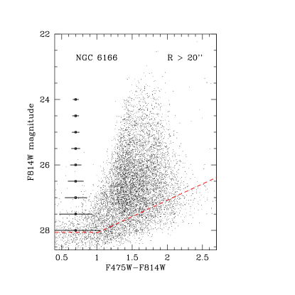
Figure 2.— Color-magnitude diagram for the globular cluster population around NGC 6166, showing the radial zone $20^{\prime\prime}-160^{\prime\prime}$ (equivalent to $R=12-100$ kpc). The red dashed line across the lower part of the diagram shows the 50% detection completeness level of the photometry, while the errorbars along the left show the measurement uncertainties in the color index.

We started the data analysis from the $*.flc$ files provided by the HST Archive. With stsdas/multidrizzle a single combined image was then generated in each filter which was CTE-corrected, mostly free of cosmic rays, and corrected for geometric distortion. Photometry was carried out with the standard tools in SourceExtractor (SE; Bertin & Arnouts, 1996) and DAOPHOT (Stetson, 1987) in its IRAF implementation, including aperture photometry (phot) followed by PSF fitting through allstar. First, the images in both filters were registered and combined to produce a master white-light image, then SE was run on that master image to produce a very deep finding list of objects. This list was used as input to daophot/phot for the images in both filters. Clearly nonstellar or crowded objects were deleted through the use of SE and allstar parameters: specifically, objects were kept if within $0.9<r_{1/2}<1.4$ px, $\chi<2$, and $err<0.3$ mag. See Harris (2009a) for detailed examples of the procedure.

The PSFs were empirically generated from bright, uncrowded starlike objects distributed across the target fields. For the ACS fields, 95 stars in $F475W$ and 87 stars in $F814W$ were summed to generate the PSFs, while for WFC3 42 stars in $F475W$ and 39 stars in $F814W$ were used. The PSF shape was set to be quadratically variable in position $(x,y)$, though comparisons with the uniform-PSF option showed negligible differences in the resulting photometry. The PSF-fitted magnitudes were corrected to large-aperture magnitudes ($r=0.5\arcsec$) with aperture photometry of bright isolated stars, and lastly corrected to total magnitudes with the enclosed-energy curves published in the ACS/WFC and WFC3 Handbooks.

The final data list consists of starlike objects that were measurable on both filters, and that had $(x,y)$ positions matching between filters to within 0.1 arcsecond. We report our results in the natural filter-based magnitudes $F475W,F814W$ and in the VEGAMAG system. Values for the filter zeropoints given on the HST webpages appropriate for the dates of the exposures have been used as follows: $F475W_{0}$ = 25.778 (WFC3) or 26.154 (ACS), $F814W_{0}$ = 24.680 (WFC3) or 25.523 (ACS). The color index $(F475W-F814W)$ is close to $(g-I)$, but can also be transformed to $(B-I)$ through (Saha et al., 2011)

$$(B-I)\, = \,1.185\,(F475W-F814W),$$

$$I\, = \,F814W+0.014\,(B-I)\,.$$ (1)

In Figure 1, the $xy$ locations of the 8223 objects brighter than $F814W=27.2$ (clearly brighter than the photometric completeness limit, as discussed in the next section), are plotted. The field also contains some companion galaxies in A2199, the three brightest of which are NGC 6166D (at upper left in Fig. 1), NGC 6166A (on the lower left edge), and PGC058261 (left of center). These are marked in the Figure with small circles of radii $10^{\prime\prime}$. These appear to have small GC populations of their own, but clearly make up very minor additions to the overwhelmingly larger population around NGC 6166 itself. In the very center ($R<10^{\prime\prime}$) we find the well known “multiple nucleus” of NGC 6166 where three small cluster galaxies lie in projection against its central bulge. Analysis of their light profiles (see B15) indicates that these companions are relatively undistorted and thus not physically connected with the central BCG.

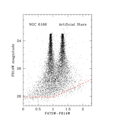
Figure 3.— Color-magnitude diagram for artificial stars in the ACS/WFC field around NGC 6166. The measured stars here are ones falling in the radial zone $R>20^{\prime\prime}$. Fake stars were inserted with magnitudes and colors falling on two dispersionless vertical sequences, so the measured scatter in color seen in this Figure represents the internal measurement uncertainty. The red dashed line across the lower part of the diagram shows the 50% detection completeness level of the photometry as in Fig. 2.

The final color-magnitude diagram for the starlike objects in the ACS field is shown in Figure 2. It includes 11371 objects in the radial range $R>20^{\prime\prime}$ and excludes the $10^{\prime\prime}$ regions around the three companion galaxies as defined in Fig. 1. An enormous GC system is present, but the spread in color is large, and the normal blue, metal-poor (MP) and red, metal-rich (MR) subpopulations are considerably less distinguishable than in most other galaxies. We analyse this issue more carefully in the next sections.

3. Completeness and Measurement Uncertainties

To quantify the completeness and photometric uncertainties we carried out extensive artificial-star tests through daophot/addstar, independently of similar experiments done for the luminosity-function analysis in Paper I. In a series of trials we added mock stars into the original images that were designed to mimic roughly the colors of the classic ‘blue’ and ‘red’ globular cluster sequences. The input artificial stars followed dispersionless vertical sequences separated by $\Delta(F475W-F814W)=0.40$ mag, and once added to the images, the photometric reduction followed identical procedures to the steps described above.

The measured CMD for the artificial-star experiments combining all trials is shown in Figure 3. The artificial blue and red sequences are easily distinguished from one another for any magnitudes $F814W\lesssim 26.5$; fainter than that, the sequences start to overlap because of the color spread generated purely by measurement scatter. As expected for photometry in very uncrowded fields like these, the mean measurement uncertainties estimated by allstar as a function of magnitude agree well with the estimates from these addstar runs.

The completeness function $f(m)$ is the fraction of inserted stars that were recovered by the photometry. The addstar results for $f$ are shown in Figure 4. Once outside the innermost zone $R>20^{\prime\prime}$ (400 px), no significant dependence of $f(m)$ on $R$ is seen; as described in Paper I, the field is unaffected by crowding at any radii, and the background galaxy light has already decreased below the point where it affects the completeness.

To describe the shape of the function $f$, it is useful to have an interpolation curve that follows the data simply and accurately. A sigmoid-type function of the form

$$f(m)\,=\,{1\over{1+e^{\alpha(m-m_{0})}}}$$ (2)

satisfies these criteria very well. Here, $m_{0}$ is the magnitude level at which $f=0.5$ (the 50% completeness limit) and $\alpha$ is a parameter adjusted to match the steepness of dropoff of $f(m)$ towards fainter magnitudes. This function is similar in form to the Fermi/Dirac probability distribution, and is also the same as the formula used by Alamo-Martínez et al. (2013) (see their Eq. 2) with C=0. Other and more complex functional forms can be found, e.g., in Fleming et al. (1995), Puzia et al. (1999), Barker et al. (2004), and Alamo-Martínez et al. (2013) useful for various special circumstances that fortunately do not apply here.

In Table 1 the detection completeness parameters for the region $R>20^{\prime\prime}$ centered on NGC 6166 (again, excluding only the innermost radial range near galaxy center) are summarized.

Table 1Detection Completeness Parameters

Detector	Filter	$m_{0}$	$\alpha$
ACS/WFC	F475W	29.00	2.45
	F814W	28.00	2.45
WFC3	F475W	29.40	4.16
	F814W	27.50	4.30

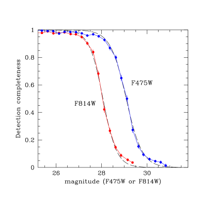
Figure 4.— Mean curves for detection completeness $f$ for the radial range $R>20^{\prime\prime}$. The interpolation function parameters are as defined in Table 1.

As noted above, the observed scatter in colors for the real objects in Fig. 2 is much larger than for the simulation in Fig. 3 and is large enough to obscure any clean division between the standard blue and red GC sequences. To test further whether or not the observed scatter is intrinsic, three of the authors (WEH, JPB, BCW) ran independent photometric reductions in different ways starting from the raw images. Comparative tests included different forms of small-aperture photometry from DAOPHOT and SE, along with selection criteria that also differed among the three reductions. All these yielded color-magnitude diagrams that showed close agreement with the allstar reductions, to well within the internal measurement uncertainties at all magnitudes. In the following analysis, we therefore continue using the allstar data.

Lastly, we emphasize that the analysis presented in the following sections relies on the magnitude range $F814W<27$, within which photometric completeness is high.

4. The WFC3 Parallel Field

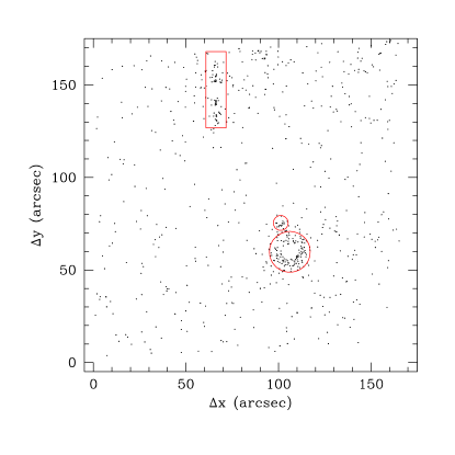
Figure 5.— Locations of measured objects in the WFC3 field with $F814W<27.2$. Axes are labelled in arcseconds. The exclusion regions around three galaxies in the field are marked as the red circles and box.

The WFC3 camera was used in Coordinated Parallel mode to image a comparison field centered at ($\alpha$ = 16:28:46.3, $\delta$ = 39:26:46.8) (J2000) through the same pair of filters. The projected distance of the WFC3 field center from NGC 6166 is $6.5^{\prime}$ SSE, equivalent to 245 kpc, and thus still well within the volume of the A2199 galaxy cluster. Coincidentally – and very usefully – the WFC3 field center is at the same radius as the outermost extent of the surface brightness profile measured by B15.

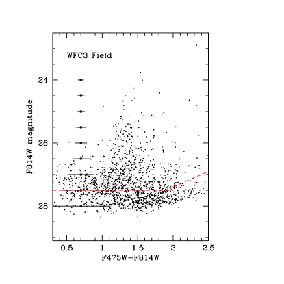
Figure 6.— Color-magnitude distribution for the starlike objects in the WFC3 field, lying outside the exclusion regions defined in the previous figure. Internal photometric uncertainties for the color indices are indicated along the left side. The red dashed line shows the 50% photometric completeness limit as determined from artificial-star tests.

Exactly the same measurement procedure as outlined above was followed. The distribution of measured starlike objects brighter than $F814W=27.2$ is shown in Figure 5. Here, excess populations of objects can be seen grouped closely around three other A2199 galaxies: these are an edge-on disk galaxy (PGC058278) near the top edge of the frame; a moderate-sized elliptical (PGC058279/282) at lower right; and a small elliptical (SDSSJ162845.08+392629.5) just above it. As shown in the Figure, exclusion regions around each of these three were drawn and objects within those regions deleted from the lists. The remaining area outside the exclusion regions is 7.294 arcmin².

Figure 6 shows the color-magnitude distribution for the starlike objects excluding the ones near these small galaxies. A population of objects is clearly present in the same range of colors and magnitudes as the GC blue sequence in Fig. 2, along with a sprinkling of redder objects. To answer how many of these are GCs that could belong either to the extended envelope of NGC 6166 or to the A2199 ICM, we need an estimate of the actual background density of starlike objects, which is addressed in the next section.

Artificial-star tests were run in the same way as for the ACS field, to determine the photometric completeness $f(m)$ and internal measurement uncertainties, with results as shown in Figure 7.

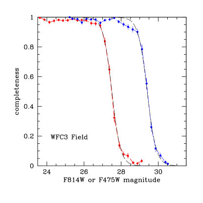
Figure 7.— Photometric completeness curves for WFC3 $F814W$ (red points) and $F475W$ (blue points). The dashed lines show the interpolation curves with parameters $m_{0},\alpha$ as listed in Table 1.

5. Assessment of Field Contamination

Ideally we would like to measure the field contamination level directly, from ACS/WFC or WFC3 images that (a) use the same filters as in our data, (b) have similar exposure times, and (c) are from pointings close to the A2199 region in a “blank field” not falling on any other cluster of galaxies. Unfortunately, images matching these criteria are hard to find in the HST Archive anywhere within several degrees of A2199, but a field that comes usefully close is from program GO-10412 (PI: Lacy). From their various ACS pointings around the sky we select their target at $\alpha=$ 16:56:47.1, $\delta=$ +38:21:36.7, which is at a projected distance of 5.55 degrees (= 12.6 Mpc) from NGC 6166. Exposure times are 1876 sec in $F475W$ and 1760 sec in $F814W$. The resulting color-magnitude diagram obtained with the same selection procedures is shown in Figure 8. Starlike objects are quite rare particularly for the range of magnitudes ($23.5\lesssim F814W\lesssim 27.0$) and color indices ($1.1<(F475W-F814W)<2.2$) that generously enclose the NGC 6166 GC population. This target box is shown in Figure 8.

Figure 8.— Color-magnitude diagram for a background field near A2199, observed with the ACS/WFC camera in $F475W,F814W$. The box outlined by dashed lines marks the approximate range of magnitudes and colors occupied by globular clusters around NGC 6166.

Aside from the shorter exposure times, a more important difference between this background field and our data is that its raw exposures used only one quadrant of the ACS/WFC array, and thus contain only a quarter of the field size we would like. Nevertheless, after scaling the areas these results suggest that no more than $\sim 20$ starlike objects contaminate the CMD within our main target GC region; and most of these will be fainter than $F814W\simeq 26.5$.

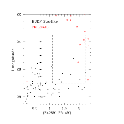
Figure 9.— Color-magnitude diagram for starlike objects measured in the HUDF (Hubble Ultra-Deep Field) (black points), and for a model population of foreground stars generated by TRILEGAL (red points; see text). As in the previous figure, the dashed box indicates the region occupied by NGC 6166 globular clusters. Errorbars at the left are the measurement uncertainties from the HUDF catalog.

As a second check, data were used from the Hubble Ultra-Deep Field (HUDF) as provided in the catalogs at heasarc.gsfc.nasa.gov/W3Browse/hst/hubbleudf.html. The HUDF data in $F435W$ and $F775W$ were transformed to $(B-I)$ with the conversions in Saha et al. (2011), and from there to $(F475W-F814W)$. To select out only starlike objects we removed any with $r_{1/2}>3.0$ px, $ell>0.3$, or $fwhm>4.1$ px, leaving just 173 objects over the ACS/WFC field area. These remaining objects ought to be a combination of Milky Way foreground stars and faint, very small-scale background galaxies at high redshift. Their color-magnitude distribution is shown in Figure 9. Although the color transformations and selection criteria are not as exact a match as we would like, the results indicate again that contamination in the target GC region is at the level of less than a dozen objects.

Finally, we have used the TRILEGAL model (Girardi et al., 2005) to simulate the expected population of Milky Way foreground stars in the direction of NGC 6166 and over the ACS/WFC field area. The results, again transformed into our filter system, are shown as the red circles in Fig. 9. No more than a handful of stars fall within the target CMD region.

In summary, the contaminating population of foreground stars is mostly brighter and redder than the NGC 6166 GC population, while the faint, small background galaxies that make it through our selection criteria are mostly fainter or bluer. The net field contamination in the GC region of the CMD is at the level of $\simeq 0.2$% and thus negligible. The overwhelming majority of the objects in Figs. 2 and 6 are the globular cluster population we are seeking. In the following analysis, we do not apply any contamination corrections. We are now in a position to investigate the spatial and metallicity distributions of the GCS.

6. Color and Metallicity Distributions

A physical division of GC populations into distinct metal-poor and metal-rich subgroups was first established clearly for the Milky Way (Zinn, 1985) by basing the division on the combination of metallicity, spatial distribution, and kinematics. Bimodality was then found in a steadily increasing list of other galaxies of every type and environment (e.g. Zepf & Ashman, 1993; Geisler et al., 1996; Gebhardt & Kissler-Patig, 1999; Larsen et al., 2001; Kundu & Whitmore, 2001; Peng et al., 2006; Harris, 2009a; Brodie et al., 2014, among dozens of other papers) and were linked to various two-phase formation scenarios for major galaxies (e.g. Ashman & Zepf, 1992; Forbes et al., 1997; Côté et al., 1998; Beasley et al., 2002; Brodie & Strader, 2006).

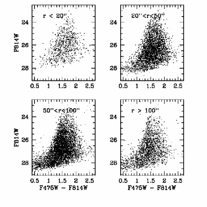
Figure 10.— Color-magnitude diagram for the globular cluster population around NGC 6166, subdivided into four radial zones.

A new round of interpretations connects the two subpopulations more directly to hierarchical-merging galaxy formation models (Kravtsov & Gnedin, 2005; Muratov & Gnedin, 2010; Tonini, 2013; Li & Gnedin, 2014). Old, metal-poor clusters in a large galaxy formed both within the gas-rich pregalactic dwarfs at the beginning of the merger tree (redshifts $z\gtrsim 4$), and within dwarf satellite galaxies that were later accreted by the continuously growing central giant. By contrast, metal-rich clusters can form either within more massive halos during the most active epoch of the merger tree ($z\sim 2-3$), or during later major mergers if such mergers bring in significant amounts of gas (see the references cited above).

6.1. Bimodality or Not? The Shape of the MDF

For galaxies well beyond the Local Group, GC metallicity measurements based directly on spectroscopic indices are difficult, so in most studies of this type, integrated color indices are used to measure large samples of GCs more efficiently. The specific transformation from color to [Fe/H] depends on the index and in some cases may be measurably nonlinear (e.g. Peng et al., 2006), but in all cases the color index increases monotonically (becomes redder) with increasing metallicity. The color distribution function (CDF) is therefore very useful as a proxy for the MDF.

In Figure 10, the CMDs for four radial zones are shown, now including the inner region $R<20^{\prime\prime}$ and extending to the boundaries of the ACS field. The bluer clusters ($(F475W-F814W)\lesssim 1.6$) become relatively more prominent at larger radii, continuing outward to the WFC3 outer field where they are completely dominant. Thus with or without bimodality, a radial metallicity gradient is present, as is the case for most GCSs (e.g. Geisler et al., 1996; Rhode & Zepf, 2004; Larsen et al., 2001; Harris, 2009a, b; Usher et al., 2013). This result will be discussed below in the details of the spatial distribution.

The more pointed question here is whether or not we can talk meaningfully about distinct metal-poor and metal-rich components given the nearly continuous spread of measured colors. We apply a two-Gaussian fit to the CDF for the subset of GCs in the magnitude and color ranges $23.0<F814W<26.5$ and $1.1<(F475W-F814W)<2.2$ using the GMM code (Gaussian Mixture Modelling; see Muratov & Gnedin, 2010). Since the sample size is large it is easily possible to carry out the fit solving for 5 free parameters: the mean colors $\mu_{1,2}$(blue,red), their Gaussian dispersions $\sigma_{1,2}$(blue,red), and the blue fraction $p_{1}\equiv N(blue)/N(tot)$.

The results, plotted on the color histogram for all radii $R$, are shown in Figure 11. The best-fit solution yields ($\mu_{1}=1.401\pm 0.010$, $\mu_{2}=1.715\pm 0.015$) for the means, ($\sigma_{1}=0.121\pm 0.005$, $\sigma_{2}=0.178\pm 0.006$) for the dispersions, and $p_{1}=0.422\pm 0.038$ for the blue fraction. Uncertainties in the fitted quantities were determined through bootstrapping. (Note that the values plotted in Fig. 11 are the dereddened color indices, not the raw colors.)

The bimodal Gaussian model turns out to provide an extremely close match to the data, even though the two modes are heavily overlapped. A single-Gaussian fit is strongly rejected by GMM at far above 99% significance. In addition, a trimodal model provides no improvement to the total fit, and in any case the third mode identified by GMM turns out to be on the red-side tail and makes up only 4% of the total population.

If we enforce a homoscedastic fit (same variances for both modes), as has frequently been done in the previous literature, the GMM solution yields $\mu_{1}=1.451$, $\mu_{2}=1.793$, $\sigma_{1}\equiv\sigma_{2}=0.147$, $p_{1}=0.609$. This result is shown in Figure 12. This second solution does not do as well especially at matching the blue peak and intermediate color range, and the heteroscedastic model (different variances) is strongly preferred by GMM at a $>$99.9% level of significance. In addition, we have no a priori physical reason to impose equal variances. As noted by Peng et al. (2006), the forced assumption $\sigma_{1}\equiv\sigma_{2}$ often has the unwanted consequence of driving the estimated peaks $\mu_{1,2}$ away from their true values. The most striking difference between the two fits is the surprisingly large change in the relative numbers of clusters in each mode: imposing equal variances increases the ratio $p_{1}$ from 0.42 to 0.61. A difference this large was numerically possible essentially because of the overlap between the two modes.

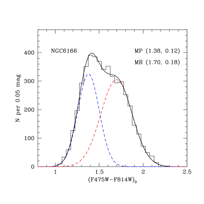
Figure 11.— Color histogram for dereddened color indices of the NGC 6166 globular clusters, in bins of 0.05 mag. All clusters in the ACS field brighter than $F814W=26.5$ at all radii are included. A best-fit bimodal Gaussian model is superimposed, where the metal-poor component is shown as the blue dashed line, the metal-rich component as the red dashed line, and their sum as the solid line. The mean and dispersion of the two components are given at upper right.

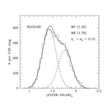
Figure 12.— Color distribution for the NGC 6166 GCs, with a bimodal Gaussian where both components are required to have the same variance (homoscedastic).

As a check of the numerics we have also used the multimodal fitting code RMIX (see Wehner et al., 2008; Harris, 2009a), which yielded results completely consistent with GMM. RMIX permits the use of any number of modes, as well as other non-Gaussian asymmetric functions such as Poisson or gamma functions, but none of these yield improvements on the bimodal Gaussian model.

Table 2Bimodal Gaussian Fits by Radial Range

$R$ Range	$n$	$\mu_{1}(\pm)$	$\mu_{2}(\pm)$	$\sigma_{1}(\pm)$	$\sigma_{2}(\pm)$	$p_{1}(\pm)$
$<20^{\prime\prime}$	558	1.386(0.055)	1.755(0.038)	0.129(0.023)	0.178(0.016)	0.29(0.12)
$20^{\prime\prime}-40^{\prime\prime}$	1138	1.442(0.036)	1.757(0.128)	0.128(0.014)	0.178(0.015)	0.35(0.11)
$40^{\prime\prime}-70^{\prime\prime}$	1509	1.457(0.021)	1.763(0.036)	0.133(0.009)	0.176(0.013)	0.48(0.09)
$70^{\prime\prime}-100^{\prime\prime}$	945	1.419(0.016)	1.741(0.035)	0.114(0.010)	0.168(0.015)	0.52(0.07)
$100^{\prime\prime}-165^{\prime\prime}$	611	1.400(0.013)	1.705(0.031)	0.111(0.007)	0.170(0.015)	0.55(0.07)
$390^{\prime\prime}$ (WFC3)	147	1.324(0.021)	1.674(0.074)	0.136(0.033)	0.244(0.013)	0.71(0.12)

Table 3Bimodal Gaussian Fits by Magnitude Interval

$F814W$ Range	$n$	$\mu_{1}(\pm)$	$\mu_{2}(\pm)$	$\sigma_{1}(\pm)$	$\sigma_{2}(\pm)$	$p_{1}(\pm)$
23.0-24.0	139		1.679(0.013)		0.141(0.011)	0.00
24.0-24.5	257	1.445(0.011)	1.687(0.020)	0.039(0.011)	0.158(0.011)	0.22(0.06)
24.5-25.0	531	1.431(0.021)	1.680(0.032)	0.066(0.018)	0.173(0.014)	0.22(0.10)
25.0-25.5	848	1.456(0.019)	1.784(0.029)	0.112(0.009)	0.158(0.014)	0.46(0.07)
25.5-26.0	1255	1.426(0.016)	1.781(0.026)	0.122(0.008)	0.167(0.012)	0.50(0.06)
26.0-26.5	1738	1.380(0.017)	1.708(0.025)	0.119(0.009)	0.206(0.008)	0.37(0.06)
26.5-27.0	2044	1.348(0.017)	1.708(0.023)	0.125(0.008)	0.220(0.008)	0.41(0.05)
23.0-26.5 (PSF)	4712	1.401(0.009)	1.719(0.015)	0.122(0.005)	0.178(0.006)	0.42(0.04)
23.0-26.5 (ap)	3696	1.464(0.011)	1.783(0.017)	0.123(0.006)	0.163(0.008)	0.48(0.04)

6.2. Color (Metallicity) versus Radius and Luminosity

GMM fitting results for samples subdivided by radial zone $R$, and by magnitude range $F814W$, are listed in Tables 2 and 3, and the full histograms are displayed in Figures 13 and 14. For the radial zones in Table 2, the data in the range $23.0<F814W<26.5$ and $1.1<(F475W-F814W)<2.2$ are used. Successive columns give (1) the zone boundaries in arcseconds; (2) the total number of GCs in the range; (3,4) the means and uncertainties of the blue and red modes; (5,6) the standard deviations of the blue and red modes and their uncertainties; and (7) the blue GC fraction $p_{1}$.

The last line in Table 2 gives the parameters for the WFC3 field: here, two modes are still present and both modes are nominally slightly bluer than in the ACS radial bins. However, we believe it is risky to conclude that these differences are intrinsic, given the remaining uncertainties in the filter zeropoints of both cameras, and the internal zeropoint corrections of the PSF-based photometry to large apertures.

The last two lines in Table 3 give the GMM fit parameters derived separately from the allstar PSF-fitting photometry, and then the small-aperture photometry described above. The zero-point calibrations for the aperture photometry were only approximate and thus account for the differences in $\mu_{1},\mu_{2}$; more importantly, the internal dispersions $\sigma_{1},\sigma_{2}$ are nearly identical from both methods, indicating again that the observed color spread is not an artifact of the photometric method.

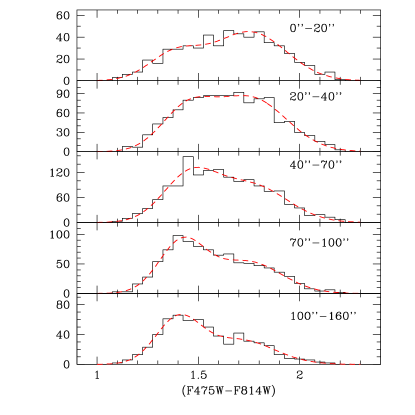
Figure 13.— Color histograms for radial zones centered on NGC 6166. In each panel the dashed red line gives the best-fit bimodal Gaussian solution from GMM, with parameters as given in Table 2. A strong radial metallicity gradient is present, driven by the changing ratio of blue to red GCs with $R$.

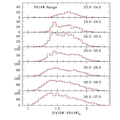
Figure 14.— Color histograms for GCs over all radii but subdivided by magnitude. The dashed red line in each panel shows the best-fit bimodal Gaussian solution from GMM, with parameters given in Table 3. Note the shift towards a unimodal distribution in the brightest bin.

Finally, in Figure 15 we show the GC intrinsic color versus radius $R$, for all GCs brighter than $I=27$. Dividing the sample into two at $(F475W-F814W)=1.55$ (see below), and then carrying out a solution for mean color versus log $R$, yields $\langle F475W-F814W\rangle_{0}(blue)\,=\,(1.37\pm 0.01)-(0.003\pm 0.007)logR^{\prime\prime}$ and $\langle F475W-F814W\rangle_{0}(red)\,=\,(1.83\pm 0.02)-(0.045\pm 0.009)logR^{\prime\prime}$. The mean color of the MP population shows no significant change with radius, while the MR population exhibits a shallow but significant negative gradient equivalent to a heavy-element abundance gradient $Z\sim R^{-0.14\pm 0.03}$. By contrast, the GCSs of many other giant galaxies show negative metallicity gradients of similar amplitudes in both their MP and MR components (Geisler et al., 1996; Forte et al., 2001; Lee et al., 2008; Harris, 2009a, b; Hargis & Rhode, 2014). For NGC 6166, the overall metallicity gradient in the global GCS is generated primarily by a “population gradient” of the changing ratio of blue to red GCs.

The absence of a metallicity gradient for the MP clusters is suggestive of strong mixing of the cluster sub-populations brought by former satellite galaxies accreted by the central host. Recently Monachesi et al. (2015) have found that Milky-Way-type disk galaxies display a wide range of halo metallicity gradients out to remarkably large radius ($\sim 50$ kpc or more than 10 effective radii). They find that large galaxy-to-galaxy differences also exist in the width (intrinsic dispersion) of the halo-star MDFs. For giant galaxies like the BCGs that may have accreted many disk galaxies or stripped stars via harassment, this material is consistent with the idea that their halos would have ended up with strongly mixed stellar populations and weak global metallicity gradients.

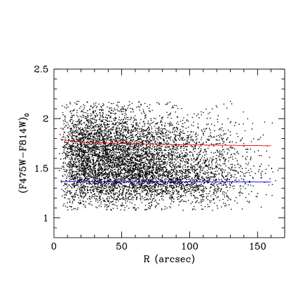
Figure 15.— Dereddened color index versus radius for the GCs in NGC 6166. The blue and red lines show the solutions for color versus radius as listed in the text.

The change in blue fraction $p_{1}$ with $R$ turns out empirically to behave in an extremely simple way. The trend is shown in Figure 16, with datapoints taken from Table 2. Numerically we find an excellent fit to a logarithmic form,

$$p_{1}(N6166)\,\equiv\,N(blue)/N(tot)\,=\,0.30\,{\rm log}(29.2R/R_{eff})$$ (3)

where $R_{eff}=0.792^{\prime}=30$ kpc is the effective radius of the halo light profile (B15). This curve is shown in Figure 16, and will be used below to help derive the radial profiles of the MP and MR subsystems.

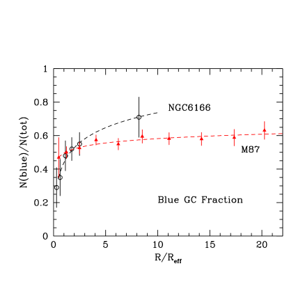
Figure 16.— Increase of the metal-poor GC fraction (NGC 6166, open circles and errorbars) with projected radius $R$. The equation for the fitted profile (dashed line) is given in the text. Solid diamonds and red dashed line give the same trend for the M87 GCS. Note that the radius is labelled in units of $R_{eff}$, the effective radius of the halo light profile.

6.3. Comparison with M87 and Other BCGs

Part of the interest in this study is the large spatial coverage of the GCS, which allows us to detect large-scale radial trends that may be difficult to see in nearer or smaller galaxies. Though similarly deep, wide-field studies are still unusual, a particularly good comparison case is M87, the Virgo BCG. We use the study of M87 carried out in the $g^{\prime},i^{\prime}$ bands from Harris (2009b) to analyze its MDF as a function of $R$ in the same way as for NGC 6166. To minimize field contamination we select the M87 data in the range $20<i^{\prime}<23$ and $0.6<(g^{\prime}-i^{\prime})<1.4$. The color histogram for 7736 total objects in this range and over projected distances $1^{\prime}<R<35^{\prime}$ (4 to 160 kpc) is shown in Figure 17. The bimodal-Gaussian GMM best-fit solution provides an excellent and well determined match to the color-index distribution, with mode peaks ($\mu_{1}=0.786\pm 0.002,\mu_{2}=1.056\pm 0.007$), dispersions ($\sigma_{1}=0.073\pm 0.002,\sigma_{2}=0.142\pm 0.003$), and blue fraction $p_{1}=0.541\pm 0.015$.

The two modes in M87 are more distinct and better separated than for NGC 6166. An objective measure of the separation is the $D-$statistic (Muratov & Gnedin, 2010),

$$D\,=\,{{(\mu_{2}-\mu_{1})}\over{[(\sigma_{1}^{2}+\sigma_{2}^{2})/2]^{1/2}}}\,.$$ (4)

For M87, $D=2.39\pm 0.08$ whereas for NGC 6166, $D=2.08\pm 0.12$. Both are above the $D\simeq 2$ threshold that indicates intrinsic bimodality, but NGC 6166 has relatively broader MP and MR components that cause stronger overlap.

Bimodal fits to the M87 distribution were done for several radial zones, with the resulting trend for $p_{1}$ as shown in Fig. 16. As for NGC 6166, the smooth increase in $p_{1}$ with $R$ matches a logarithmic form quite well:

$$p_{1}(M87)\,=\,0.087\,{\rm log}(4.9\times 10^{5}~{}R/R_{eff})\,$$ (5)

where $R_{eff}(M87)=1.58^{\prime}=7.4$ kpc. In units of $R_{eff}$, we can trace $p_{1}$ out further for M87, but its outward increase is distinctly shallower. The Virgo cluster is dynamically younger than A2199, still actively accreting galaxies, and thus its central galaxy may have accreted fewer small satellites that would preferentially add metal-poor clusters to the M87 outer halo.

Valuable, though less detailed, comparisons of the MDF with those in other galaxies can be made after conversion from color to metallicity [Fe/H]. Various color indices have been employed in the recent literature; translations of any one of them to [Fe/H] are discussed in many papers and, in general, are not yet as accurate as we would like them to be (see Blakeslee et al., 2010; Fensch et al., 2014; Li & Gnedin, 2014; Vanderbeke et al., 2014, for illustrative discussions partly based on modelling). In some cases, particularly the $(g-z)$ index used for the Virgo and Fornax GCS surveys, the transformation to [Fe/H] has noticeable nonlinearity (Peng et al., 2006; Blakeslee et al., 2010; Vanderbeke et al., 2014; Li & Gnedin, 2014). For our index $(B-I)$, recent linear conversions to [Fe/H] are given by Barmby et al. (2000) and Harris et al. (2006) calibrated from Milky Way and M31 clusters, and are in close agreement. Within the scatter of these calibrations no nonlinearity is evident. To be consistent with the analysis of previous BCGs from Harris (2009a) we use the one in Harris et al. (2006), which transforms to

$$(F475W-F814W)_{0}\,=\,0.316{\rm[Fe/H]}+1.822\,.$$ (6)

The conversion is calibrated from 95 Milky Way GCs with well known $(B-I)$ colors, reddenings, and spectroscopic metallicities.

The converted bimodal MDF parameters are listed in Table 4, along with eight other BCGs drawn from previous papers. The successive columns are (1,2,3) galaxy name, host galaxy cluster, and luminosity, (4) the blue fraction $p_{1}$, (5,6) the dispersions for the MP and MR modes, (7) the difference $\Delta$[Fe/H] between the mean metallicities of the MP and MR modes, (8) mode separation $D$, and (9) literature source. The last line in the Table gives the mean values for the various quantities, not including NGC 6166.

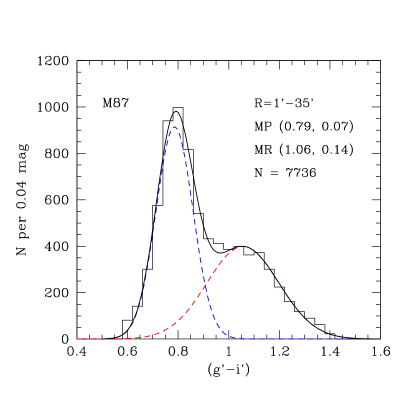
Figure 17.— Color distribution function for the GCs in M87, with data from Harris (2009b). The bimodal Gaussian fit given in the text is shown in the dashed lines, with values for the mode peaks and dispersions listed at upper right.

The other galaxies listed are the centrally dominant objects in clusters of galaxies of various richnesses, from relatively nearby groups (NGC 1407) to larger systems such as Virgo and Centaurus (M87, NGC 4696). Although other discussions of the GCSs for some of these galaxies are available (Forbes et al., 2006; Mieske et al., 2006, 2010a; Bassino et al., 2008; Peng et al., 2009; Fensch et al., 2014), the sources used here treat the MDF fits with the same methodology as our NGC 6166 analysis, and the photometry for these other galaxies has very similar internal uncertainties at the same absolute magnitude level in the CMD.

Table 4MDF Parameters for BCGs

Galaxy	Host Cluster	$M_{V}^{T}$	$p_{1}$	$\sigma_{1}$(dex)	$\sigma_{2}$(dex)	$\Delta$[Fe/H]	$D$	Source
NGC 6166	A2199	$-23.7$	0.57	0.39	0.56	1.01	2.08	1
M87	Virgo	$-22.42$	0.54	0.24	0.29	0.91	2.39	2
NGC 1399	Fornax	$-22.02$	0.63	0.23	0.36	0.94	3.11	3
NGC 1407	Eridanus	$-22.35$	0.33	0.28	0.39	1.18	3.10	4
NGC 3348	CfA 69	$-22.13$	0.49	0.20	0.42	1.09	2.95	4
NGC 3258	Antlia	$-21.87$	0.52	0.23	0.38	0.98	3.08	4
NGC 3268	Antlia	$-21.96$	0.48	0.19	0.45	0.93	3.03	4
NGC 4696	Cen30	$-23.31$	0.51	0.26	0.45	1.00	2.87	4
NGC 7626	Pegasus I	$-22.35$	0.35	0.28	0.42	1.13	2.86	4
Mean		$-22.30$	0.48	0.24	0.40	1.02

Small differences in photometric zeropoint calibrations for the various color indices used in these different studies, plus subsequent transformation into metallicity, make it difficult to compare the absolute [Fe/H](MP,MR) values meaningfully (see also Usher et al., 2015, for discussion of intrinsic galaxy-to-galaxy scatter in the correlations between color and spectral indices). The more robust results are the ones in the Table, i.e. the dispersions $\sigma(MP,MR)$ and the offsets $\Delta$[Fe/H] between the two modes, along with the resulting $D-$statistic. NGC 6166 is the most luminous BCG in the list, and it has the broadest metallicity dispersions for both MP and MR components of all galaxies in the list. However, the mean metallicity difference between the MP and MR modes is virtually identical for all of them, at $\langle\Delta$[Fe/H]$\rangle=1.0$ dex.

The very high intrinsic dispersions that we see in the NGC 6166 MDF, and the remarkably consistent 1.0 dex offset between the two modes, find some theoretical motivation particularly in the recent models of Li & Gnedin (2014). In these models, GC formation is assumed to be driven by mergers between gas-rich galaxies. Clusters inherit the metallicity of their parent galaxy at the moment of formation, which is calculated via the observed relation between galaxy stellar mass and mean metallicity. The bulk of the metal-poor clusters come from almost continuous, early mergers among small halos at the epochs when they are extremely gas-rich. To create a GC that is massive enough to survive dynamical disruption until the present, the galaxy mass needs to be above a certain threshold, $\gtrsim 10^{9}M_{\sun}$, which in turn sets the minimum metallicity. The red GCs are contributed by more massive galaxies, in which the metallicity scales weakly with mass. Thus, the mean metallicities of the MP and MR modes increase only slightly with galaxy mass, maintaining a $\sim 1$ dex offset close to what is observed. In contrast, the dispersions of both modes increase with galaxy mass, as the numbers of contributing mergers increase. This can be seen in Figures 6 and 13 in Li & Gnedin (2014). For the giant, central cluster galaxies, both MP and MR modes are so wide that they form one broad distribution, reminiscent of what we see for NGC 6166.

6.4. Mass-Metallicity Relations

A more recently discovered feature of interest is the trend of mean metallicity with GC luminosity. In several large galaxies, along the blue MP sequence especially, the mean metallicity has been observed to increase gradually with GC mass (Harris et al., 2006; Strader et al., 2006; Mieske et al., 2006; Wehner et al., 2008; Harris, 2009a; Peng et al., 2009; Cockcroft et al., 2009; Fensch et al., 2014, among others). This mass-metallicity relation (MMR) is subtle enough that it is still unclear if the effect is a simple power law (that is, if we can write $Z\sim M^{\gamma}$ for heavy-element abundance $Z$ with $\gamma=const$), or if the index $\gamma$ itself increases with mass such that the MP sequence curves more strongly toward the MR sequence at progressively higher mass.

The amplitude of the effect may also differ from one galaxy to another, and may be virtually absent in some cases, notably NGC 4472 and NGC 1399 (Strader et al., 2006; Mieske et al., 2006; Forte et al., 2007). In addition, for some galaxies (like M87 or NGC 4696) the MP sequence shows a steady near-linear slope in color toward the red for the brightest $2-3$ magnitudes of the GCLF, but in others such as NGC 1399 or NGC 4696, above a certain threshold luminosity near $2\times 10^{6}L_{\odot}$, the total CDF becomes broad and unimodal rather than bimodal (e.g. Dirsch et al., 2003; Bassino et al., 2006; Harris, 2009a).

Empirically, the effect is most noticeable for BCGs where the GCLF is rich enough to populate the highest mass range $M>10^{6}M_{\odot}$ thoroughly. For that reason, in smaller galaxies any MMR is extremely difficult to identify. For example, in the Milky Way the only individual GC that lies clearly in this high-mass regime is $\omega$ Centauri, an object that is well known to contain a complex set of stellar subpopulations more extreme than in any lower-mass GC (e.g. Bellini et al., 2009).

Theory addressing the MMR phenomenon is still in early stages. A model based on internal GC self-enrichment (Bailin & Harris, 2009) is capable of matching some of the various forms taken by the MMR (see Mieske et al., 2006, 2010b; Fensch et al., 2014). One of the strongest motivations for pursuing models involving some form of extra enrichment that increases with GC mass is that the MMR is visible along the blue GC sequence but not the red sequence. If some extra heavy elements are added to a GC in amounts depending only on its mass, the visible effect on the integrated colors can be quite noticeable for a GC that was originally very metal-poor, but nearly negligible for one that was already metal-rich. However, because it is driven by local conditions inside the GC during its formation, the Bailin/Harris model has difficulty reproducing the wide range of MMR slopes seen in different galaxies, which suggests that some environmental feature must also be at work. Large galaxies with no MMR slope, and those with broad unimodal MDFs at high GC mass, also remain challenging for this type of model.

VanDalfsen & Harris (2004) and Forte et al. (2007) adopt a simpler numerical approach to model the MDF that invokes what is essentially pre-enrichment. They model the MDF of each of the blue and red GCs as $dn/dZ\sim exp[-(Z-Z_{i})/Z_{s}]$ for the distribution of heavy-element abundance $Z$, where the free parameters are the initial or minimum allowed GC metallicity $Z_{i}$ and a scale $Z_{s}$. This form is analogous to the Simple Model of chemical evolution where $Z_{s}$ represents an effective yield. VanDalfsen & Harris assumed that $Z_{i}$ for each sequence does not change with GC mass. But Forte et al. note that if $Z_{i}$ is a function of GC mass, i.e. if more massive clusters are formed from more enriched gas, then a MMR with a range of observed forms can be reproduced. Again, however, it is not immediately obvious how MMRs of widely different slopes might be understood physically in this picture, or indeed why more massive GCs formed preferentially from regions of more enriched dense gas.

Does NGC 6166 display this phenomenon? A simple approach would be to divide the sample at $(F475W-F814W)=1.55$ where the two components cross (Fig. 11) and then derive the trend of color with luminosity without magnitude-binning (though this approach will tend to smooth over any smaller-scale variations with luminosity). Linear solutions give derived slopes $\Delta(475-814)/\Delta(mag)=-0.032\pm 0.004$ (blue) and $\Delta(475-814)/\Delta(mag)=0.002\pm 0.005$ (red), which translate into $\gamma(\rm blue)=0.25\pm 0.03$ and $\gamma(\rm red)=-0.02\pm 0.04$. Quadratic polynomial fits were also tried, but were not visibly different. These correlations are valid for $F814W<27$ ($M_{I}\lesssim-8.6$, or $M\gtrsim 2\times 10^{5}M_{\odot}$), which is near the turnover (peak) of the GCLF.

A more rigorous approach that would specifically account for the overlap between MP and MR modes, as well as their different dispersions, is to define mean points $(\mu_{1},\mu_{2})$ as a function of magnitude through bimodal-Gaussian fitting in relatively small magnitude bins. The mean points can then be used to define any systematic trend with magnitude. Mean points in $0.2-$mag intervals derived this way are superimposed on the CMD in Figure 18. A linear fit to each set of points then gives $\Delta(475-814)/\Delta(mag)=-0.037\pm 0.008$ (blue) and $\Delta(475-814)/\Delta(mag)=0.005\pm 0.007$ (red), or $\gamma(\rm blue)=0.29\pm 0.06$ and $\gamma(\rm red)=-0.04\pm 0.05$. The slopes obtained through either method are closely consistent. On the MR sequence, in rough terms there is no significant change in mean color over almost 4 magnitudes in luminosity: but in more detail, the trend in color is not a simple one and may not even be monotonic.

Along the MP sequence, however, a more consistent signal shows up indicating that a modest MMR is present. The slope $\gamma\simeq 0.25-0.3$ is near the middle of the range seen in other large ellipticals (Harris, 2009a; Cockcroft et al., 2009; Peng et al., 2009; Fensch et al., 2014). A particularly good comparison is with M87, where the blue sequence has $\gamma=0.25\pm 0.05$ for the luminosity range $M_{I}\lesssim-9$ (Harris, 2009b; Peng et al., 2009), very similar to what we find here. Notably however, in both these galaxies the slope $\gamma$ shows no indication of increasing with luminosity. A constant $\gamma$ is inconsistent with the basic self-enrichment model (Bailin & Harris, 2009), which requires curvature in the MP sequence starting with a near-vertical base below about $10^{6}M_{\odot}$ (see also Mieske et al., 2010b, for other quantitative examples).

We note that for $F814W<24.0$ (top panel of Fig. 14), the blue sequence fades out but the red sequence continues to still higher luminosity. In this magnitude range, a unimodal Gaussian function for the color distribution can be rejected at only the 92% significance level, whereas in all other luminosity bins a single Gaussian is rejected at $>99$% confidence. $F814W\simeq I<24.0$ corresponds to $L$ $\gtrsim 1.9\times 10^{6}L_{\odot}$ or a mass range $M\gtrsim 3.7\times 10^{6}M_{\odot}$ for $(M/L)\simeq 2$ (McLaughlin & van der Marel, 2005). As seen in Fig. 10, most of these high-luminosity red GCs are in the inner $\simeq 50$ kpc. A very similar trend for the red sequence to reach higher is seen in some other BCGs such as NGC 3311 (Wehner & Harris, 2007) and NGC 4874 (Harris et al., 2009), though other BCGs do not show it and thus it does not seem to be universal.

A potentially connected observation is that dwarf galaxies, which contain primarily blue MP clusters, also have GCLFs that are narrower and less extended to high luminosities than in giant galaxies (Villegas et al., 2010). Thus, any part of the GC population accreted at later times from dwarf satellites would have added to the blue GC total but would not have added ones at the highest luminosities. In the context of formation models (Li & Gnedin, 2014) larger galaxies contribute more clusters, with higher metallicity. They populate the cluster luminosity function to higher luminosities, and therefore, the brightest clusters are expected on average to be red.

The MMR phenomenon makes it clear that there is much we do not yet understand about the formation processes and internal enrichment histories of massive star clusters, particularly in the regime above $\sim 10^{6}M_{\odot}$. Additional physically motivated theory is still needed to fully explain the MMR patterns in different galaxies.

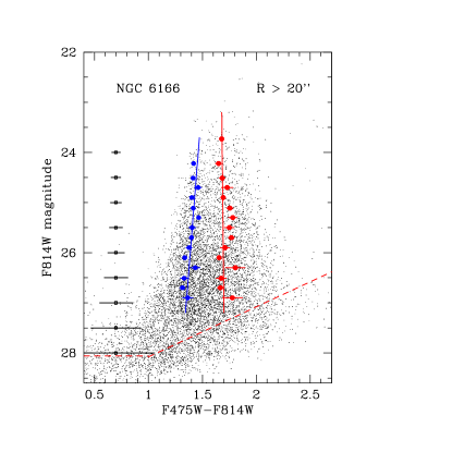
Figure 18.— Color-magnitude data for the NGC 6166 GCs, now with the mean GC color in magnitude bins taken from Table 3.

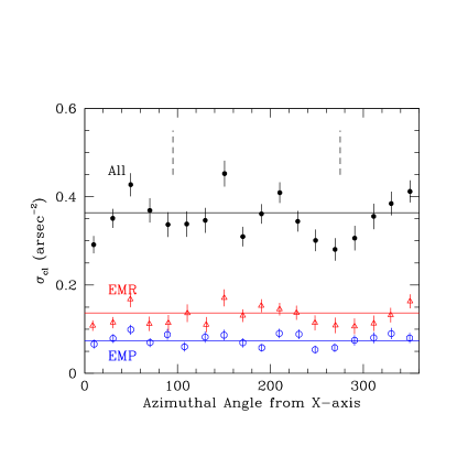
Figure 19.— Assessment of the distribution of GCs around NGC 6166 by azimuthal angle $\theta$. The density (number per arcsec^-2) of GCs in the magnitude range $F814W<27.2$ and in the radial range $20^{\prime\prime}<R<70$ is plotted in $20^{o}$ sectors. Black solid points: GCs of all metallicities. Red triangles: Extreme metal-rich (EMR) GCs. Blue circles: Extreme metal-poor (EMP) clusters. Mean values for each sample are shown as the horizontal lines. The vertical dashed lines at top mark the orientation angle of the isophotal minor axis; if the GCS follows the same orientation as the halo light, then the cluster counts should be lowest at those angles.

7. The Spatial Distribution: Halo Light Versus GCS

The GCS around this supergiant galaxy is clearly very extended, continuing out well past the outer boundary of the ACS/WFC field and on through the WFC3 field. B15 showed that the same is true for the integrated halo light. How well do these two types of stellar halo populations match up, and is the correlation affected by GC metallicity?

Evaluating the effects of metallicity is made difficult by the heavy overlap between MP and MR components. To help isolate the metallicity trends more clearly, we therefore define two GC subsamples: an “Extreme Metal-Poor” (EMP) sample with color indices bluer than the peak of the MP component ($(F475W-F814W)<1.401$); and an “Extreme Metal-Rich” (EMR) sample with colors redder than the peak of the MR component ($(F475W-F814W)>1.715$). This culling guarantees that the EMP component is minimally contaminated by overlap with the MR clusters, and vice versa for the EMR component (see Forte et al., 2007, for a similar treatment of NGC 1399 and M87). As well as testing the entire GC system, we can then determine the azimuthal and radial distributions of its extreme low- and high-metallicity components.

7.1. Azimuthal Dependence

The surface brightness (SB) profile of the NGC 6166 stellar halo changes shape significantly with radius (B15); it is nearly round in the inner halo but elongates to an ellipticity $1-(b/a)=\epsilon\lesssim 0.5$ at the outermost radii of their data. However, the position angle of the isophotal major axis stays nearly constant at $\sim 30^{o}$ E of N. Before attempting to match up the radial distribution of the halo light with the GC counts, we should therefore determine if they have similar azimuthal distributions.

In the range $R=20^{\prime\prime}-70^{\prime\prime}$ ($12-45$ kpc) we can work with a sample of GC counts that is azimuthally complete (i.e. completely enclosed in the ACS field; though we do not make the second-order corrections for the small gap between the two ACS detectors or the $10^{\prime\prime}$ exclusion circle around the satellite galaxy). In Figure 19, the number density of GCs in this radial range and with $F814W<27.2$ is shown plotted versus position angle $\theta$ relative to the x-axis of the ACS field. The counts are made in $20^{o}$ sectors. The translation between $\theta$ and the fiducial directions on the sky is that North lies $28^{o}$ clockwise from (i.e. below) the x-axis and East lies $28^{o}$ clockwise from the y-axis. By using the iterative method of moments discussed by McLaughlin et al. (1994), we find the following results:

1. For all GCs combined, the mean ellipticity is $\epsilon=0.26\pm 0.06$ with major axis at $(45\pm 11)^{o}$ E of N.

2. For the EMP GCs, $\epsilon=0.17\pm 0.13$ with major axis at $(63\pm 74)^{o}$ E of N. As is also evident from Fig. 19, both parameters are weakly determined and the assumption that the EMP cluster distribution is intrinsically spherical cannot be clearly rejected.

3. For the EMR GCs, $\epsilon=0.33\pm 0.11$ with major axis at $(42\pm 10)^{o}$ E of N.

These results indicate that the azimuthal shape of the GCS depends on metallicity. Over the same radial range $20^{\prime\prime}-70^{\prime\prime}$, the halo light ellipticity increases from $\epsilon\simeq 0.25$ to 0.37, and is oriented $\simeq 33^{o}$ E of N with only $\pm 2^{o}$ variation. The azimuthal parameters of the halo light thus closely resemble those of the EMR clusters, but not the EMP clusters.

7.2. Radial Dependence

Isophotal contours for galaxy halos are routinely measured by ellipse fitting. By contrast, GC counts are usually done in circular annuli. Any noncircularity in the GC distribution can be clearly gauged only for cases of extremely elliptical distributions, or for galaxies like BCGs where the statistical sample of GCs is very large. Even so, is difficult to calculate both radial and azimuthal parameters in fine radial steps as is done for the halo light (McLaughlin et al., 1994).

This issue is not of major importance for galaxies in which both GCS and halo light have small ellipticities. But in NGC 6166, the halo light becomes quite elongated at large radius, so we correct the SB profile $\mu_{V}$ back to an equivalent circular form that can then be directly matched to the GCS profile. For each elliptical annulus $a$ for which $\mu_{V}$ and $e$ are tabulated (as given in Table 3 of B15), we then calculate the radius $R_{eq}=\sqrt{ab}$ of the circular annulus that has the same mean surface brightness averaged around the circle, i.e. ${\langle\mu_{V}(R_{eq},\theta)\rangle}_{\theta}=\mu_{V}(a)$ where $\theta$ is the azimuthal angle of any point on the circle (see, e.g., Carter, 1978; Bender et al., 1988; McLaughlin et al., 1994).

Figure 20 shows this circularly-adjusted $\mu_{V}$ profile in comparison with the number density of all GCs, $\sigma_{cl}(R)$. The GC sample includes those in the magnitude range $23<F814W<27$, over which the photometric completeness is high for both ACS and WFC3. As before, we have assumed zero field contamination (see Section 5). The outermost datapoint in Fig. 20 is the value for the entire WFC3 comparison field. The five innermost points all lie within $R\lesssim 20^{\prime\prime}$, for which the measurements become progressively less complete and less certain.

For $R>20^{\prime\prime}$ where the completeness is high, a simple power-law decline does not accurately match the shape of the GCS profile. Instead, we try a Sérsic-type function in its classic form (Sersic, 1968),

$$\sigma_{cl}\,=\,\sigma_{e}{\rm exp}(-b_{n}[({R\over R_{e}})^{1/n}-1])$$ (7)

where $\sigma_{cl}$, the number of GCs per unit area, replaces the usual surface brightness $I(R)$, $R_{e}$ is the effective radius enclosing half the population, $n$ is an index giving the steepness of falloff of the profile, and $b_{n}\simeq 1.992n-0.3271$ (Caon et al., 1993; Graham & Driver, 2005). Using the datapoints for $R>20^{\prime\prime}$, we solve for the free parameters ($n,R_{e},\sigma_{e}$) by weighted $\chi^{2}$ minimization. For the total GC population (solid black circles in Fig. 20) we find a best-fit $n=6.7$ (solid black line in the Figure), although the $\chi^{2}$ minimum is a shallow one and any $n-$values in the range $\sim 6-7$ provide good fits. Plainly, however, the GCS defines a shallower distribution than the halo light (shown as the dashed line).

There is no clear transition in the GCS profile to the ICM; or, if there is, it lies further out than $R\sim 300$ kpc. Similarly, B15 conclude that “… the cD halo is not distinguishable using photometry alone”. This feature is in contrast to the Coma cluster, where Peng et al. (2011) found the GCS profile in NGC 4874 to become rather suddenly flatter beyond $R\gtrsim 150$ kpc. At larger radii the Coma IGC population dominates, adding up to perhaps twice as many GCs as ones belonging to the central galaxy. Interestingly however, Peng et al. (2011) also find that in the IGC population, MP GCs outnumber MR ones by 4:1, not unlike the ratio we find here for our outer WFC3 field (Table 2).

In Figure 20, we also show the EMP and EMR subsamples of clusters separately. Sérsic fits to these components give $n(EMP)\simeq 7.6$, $n(EMR)\simeq 6.8$. The EMP population is strikingly more extended than the EMR one. For purposes of rough comparison, in power-law form where $\sigma_{cl}\sim R^{\alpha}$, we find $\alpha\simeq-1.0$ (EMP) but $\alpha\simeq-1.8$ (EMR). The shallow MP slope is close to an isothermal profile that would characterize a dark-matter halo. The crossover radius where $\sigma(EMP)=\sigma(EMR)$ is at $R\simeq 50$ kpc.

Notably, the radial profile for the EMR population tracks the profile for the halo light much more closely. The adjusted halo light profile is shown as the dashed line, normalized to the EMR GCS. The normalization factor is that 1 metal-rich GC brighter than $F814W=27$ is equivalent to a halo luminosity $V=21.95$ (or $M_{V}=-13.6$). For the entire range $R>20^{\prime\prime}$, little or no significant difference can be seen between them. The outermost datapoint for the EMR sample can be seen to lie somewhat above the outward extrapolation of $\mu_{V}(R_{eq})$, but it is not clear how much weight should be put on it. That datapoint comes from only the WFC3 field and thus belongs to a very small range $\Delta\theta$ of azimuthal angle, so it is difficult to define a valid $R_{eq}$ for that radius, particularly because we also do not know the axial ratio of the GCS there.

To this result we can add the observation by B15 that the integrated $V-I$ color of the halo gradually decreases with radius, by 0.1 mag out to $R=80^{\prime\prime}$ (50 kpc). Notably, a plot of $\mu_{I}$ if extrapolated outward would look slightly shallower than $\mu_{V}$ and would bring the agreement with $\sigma_{cl}(EMR)$ even closer.

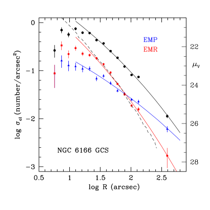
Figure 20.— Radial profiles for the globular cluster system around NGC 6166, and for the EMP and EMR subsystems defined in the text. The data are plotted in log-log form in units of number of GCs per arcsec² versus projected radius $R$. GCs in the magnitude range $23<F814W<27$ are included in the totals. Solid dots and line are the data for all GCs combined. Blue triangles and line are the extreme metal-poor GCs. Red squares and line are the extreme metal-rich GCs. Black dashed line: Integrated surface brightness profile $\mu_{V}(R)$ for the NGC 6166 halo, shifted vertically to align with the EMR GCs.

In their discussion of the NGC 6166 halo light, B15 find that by a radius $R\simeq 70^{\prime\prime}\simeq 45$ kpc, the halo velocity dispersion has risen to a value $\simeq 800$ km s^-1 comparable with the A2199 cluster galaxies, suggesting that the cD halo component has become dominant by that point relative to the core of the galaxy. They also find that the halo metallicity is $\alpha-$enhanced ([$\alpha$/Fe] = 0.3) out to $R=59^{\prime\prime}$, indicating fast star formation within $\sim 1$ Gyr and rapid quenching after that. The GCS data provide a way to extend this argument further out. If the ratio of MP to MR halo stars were to change with radius in the same way as the MP and MR GCs do, then the light profile in Fig. 20 would follow the total GC population, not the MR component. This comparison suggests that the stellar halo of NGC 6166 – both cD and core components – remains moderately metal-rich even at large radius.

The question these comparisons leave us with is the origin of the many thousands of metal-poor clusters at large radius. The major possibilities are that (a) the MP GCs originated at a very early stage of evolution in the many small, metal-poor halos just beginning their star formation, at a redshift when they still followed the shallow dark matter halo profile; or (b) many of them are from a later accreted population of disrupted small satellite galaxies or the outer halos of larger galaxies, the majority of which would be metal-poor GCs. Both factors can be part of the story. In either case, the argument relies on the empirical result that the GC specific frequency (number of GCs per unit halo light) increases dramatically as metallicity decreases. That is, low-metallicity environments were much more efficient at forming massive star clusters in the early universe (Harris & Harris, 2002; Forte et al., 2005; Harris et al., 2007; Kruijssen, 2014; Forte et al., 2014; Peacock et al., 2015). Accreted stellar populations dominated by dwarfs could then add GCs with only minor effects on the metal-rich halo light component.

The synthesis to be drawn from the combined data is largely in agreement with the conclusions of B15 from their surface photometry and integrated-light spectroscopy, that the extended cD-type halo of NGC 6166 consists of tidal debris from other galaxies in the cluster. These other galaxies were likely themselves to have a wide variety of halo metallicity gradients and dispersion (Monachesi et al., 2015). In the dense central environment of A2199 star formation proceeded intensely and rapidly for a short period of time, with later additions to the cD halo coming from dynamical disruption processes.

Finally, we estimate the total GC population and specific frequency $S_{N}$ (Harris & van den Bergh, 1981). The local specific frequency will increase outward since $\sigma(GCS)$ is shallower than the halo light profile, so we restrict the calculation to the outermost radius to which either component has been traced, namely $R\simeq 415^{\prime\prime}$ = 260 kpc. Integrating the GCS Sérsic profile from $20^{\prime\prime}-415^{\prime\prime}$ gives $N_{GC}=18600\pm 1000$ brighter than $F814W=27.0$. To this we add $\simeq 900$ more for $R<20^{\prime\prime}$, taking the $\sigma_{cl}$ value at $20^{\prime\prime}$ and assuming conservatively that it is constant further in. Since the limiting magnitude is almost exactly at the turnover (peak frequency) of the GCLF, this total is then doubled to account for fainter GCs, giving $N_{GC}(tot)=39000\pm 2000$. To the same outer radius, B15 calculate a total integrated $V$ magnitude $V(tot)=11.75$ or $M_{V}^{T}=-23.85$. The global specific frequency is then

$$S_{N}\,=\,N_{GC}(tot)\cdot 10^{0.4(M_{V}^{T}+15)}\,=\,11.2\pm 0.6.$$ (8)

A $S_{N}$ this large is quite similar to the values found for NGC 4874, M87, and other BCGs (Harris et al., 1995; Peng et al., 2011; Harris, 2009b). For a mean GC mass of $\sim 2\times 10^{5}M_{\odot}$, the total mass fraction of GCs to galaxy stellar mass in NGC 6166 is roughly $M(GCS)/M_{\star}\simeq 5\times 10^{-3}$.

Integrated outward to the same limiting radius $R(max)=415^{\prime\prime}$, the total numbers of blue and red GCs are $N(MP)=22300\pm 1500$ and $N(MR)=16700\pm 1400$. The global ratio $N(blue)/N(tot)$ is then $0.57\pm 0.05$.

Because the overall GCS surface density profile $\sigma_{cl}(R)$ is shallower than the surface brightness profile $I_{V}(R)$ (Fig. 20), $S_{N}$ increases outward. The quantitative trend is shown in Figure 21, obtained by integrating the appropriate Sérsic profiles for the GCS and for the $V-$band surface brightness profile from B15. For the inner halo $R\lesssim$ 40 kpc, the specific frequency is at a level $S_{N}\sim 5$ that is in the normal range for large early-type galaxies, but it rises smoothly outward to the limit of our data.

Comparisons can be made with the older published estimates obtained from ground-based imaging. Pritchet & Harris (1990) found $S_{N}\simeq 2.4\pm 1.1$ within $R\sim 20$ kpc, while we obtain $S_{N}=4.1$ to that radius. Because they used the outer parts of their $\sim 100^{\prime\prime}$ field of view to define background, it is now clear that the GCS population was oversubtracted. Bridges et al. (1996) were able to define the background count level with a much more remote control field and found $S_{N}=9(+9,-4)$ to within $\simeq 50$ kpc, whereas our value is $S_{N}(50kpc)=6.5$, within their estimated range. Lastly, Blakeslee et al. (1997) determined $S_{N}=8.2\pm 2.1$ within $R\simeq 35$ kpc through a combination of resolved-object photometry and surface brightness fluctuation measurement; by comparison we obtain $S_{N}(35kpc)=5.6$. Thus these earlier estimates have accuracies of typically a factor of two.

Figure 21.— Increase of specific frequency $S_{N}$ with radius around NGC 6166. Here, $S_{N}(R)$ is defined as the total cluster population within radius $R$, divided by the total $V-$band luminosity within $R$. The vertical dashed line shows the outer boundary for our ACS/WFC field; at larger radii the curve relies on the WFC3 data and the fitted Sérsic profile for the GCS (see text). The three points with errorbars indicate estimates in the earlier literature from ground-based imaging.

8. Summary

We have presented the first comprehensive photometric study of the extraordinarily rich globular cluster system around NGC 6166, the BCG in A2199 and a classic cD-type galaxy. Two-color photometry from the HST ACS and WFC3 cameras was used to measure the GC population with a limiting magnitude at the GCLF turnover point. Our principal findings are these:

1. The GCS is extremely populous, easily detectable out to at least 260 kpc and totalling 39,000 GCs to that radius. The global specific frequency to that radius is $S_{N}=11.2\pm 0.6$.

2. The metallicity distribution of the GCs can still be very well described by a bimodal Gaussian-type function, and these two modes are separated by $\Delta$[Fe/H] = 1.0 dex as is the norm for other galaxies. But the metal-rich and metal-poor modes both have larger dispersions in NGC 6166 than in other systems, making the two modes overlap significantly and filling the usually-sparse intermediate-metallicity zone. Both these features are reminiscent of the recent Li & Gnedin (2014) models in which GC formation is driven at every stage by halo mergers. With NGC 6166, we may be seeing the results of a hierarchical formation process so extended and complex that the simplistic bimodal, two-phase scenario is no longer an effective picture of its history. This regime of extreme galaxy mass and environmental richness is essentially populated only by BCGs.

3. The GCS shows a strong global metallicity gradient, but this results almost entirely from the decreasing ratio of MR to MP clusters with increasing radius. The mean metallicity of each mode changes little with radius.

4. The radial profile of the $V-$band halo light matches the metal-rich GCs extremely well for all radii $R>20^{\prime\prime}$ (12 kpc), falling roughly as $R^{-1.8}$ in surface intensity ($\mu_{V}$) or GC number density ($\sigma_{gc}$). By contrast, the metal-poor GCs follow a much shallower profile as $\sigma\sim R^{-1.0}$, more nearly matching an isothermal dark-matter halo. The red, metal-rich GCs lie in an elliptical spatial distribution that also matches the shape of the halo light.

5. The blue GC sequence shows a modest mass-metallicity relation where heavy-element abundance increases with cluster mass as $Z\sim M^{0.25}$. But at the highest GC luminosities ($\gtrsim 2\times 10^{6}L_{\odot}$) the red sequence reaches higher and the MDF becomes unimodal. No single physical model is yet able to account satisfactorily for the puzzling variety of MMR structures that have already been seen in large galaxies.

6. We find no clear spatial transition between the inner core galaxy and its cD envelope, or the ICM. In this respect it behaves the same way as does the halo light profile, but differs from the more abrupt transition seen in the Coma cluster and its BCG, NGC 4874.

Appendix A MDF Parameters for the Milky Way

Although the Milky Way is far from being a BCG, it represents the foundation of the bimodality paradigm for globular cluster systems. To provide a comparison for the BCGs listed in Table 4, we show the Milky Way cluster metallicities in Figure 22, based on the most recent compendium of measurements. Here, 139 clusters with reddenings $E_{B-V}<1.6$ are shown, with [Fe/H] values from Harris (1996) (2010 edition). A unique advantage of this sample is that the great majority of these metallicities are determined directly from high dispersion spectroscopy of the cluster stars.

The fitted GMM-derived parameters, this time directly in units of [Fe/H] rather than color, are $\mu_{1}=-1.55\pm 0.07$, $\mu_{2}=-0.55\pm 0.10$, dispersions $\sigma_{1}=0.38\pm 0.04$ dex, $\sigma_{2}=0.23\pm 0.05$ dex, and MP fraction $p_{1}=0.69\pm 0.09$. The effect of small-sample statistical scatter is evident in the bin-to-bin differences, but the biggest single difference between this and the BCGs is perhaps the much smaller dispersion $\sigma_{2}$ for the MR clusters. Once again, the results are suggestive of a more prolonged and dominant metal-rich formation mode in the biggest galaxies.

Interestingly, the width of the MP component (0.38 dex) is larger than for most of the BCGs listed above. This spread causes several clusters that nominally belong to the MP component to fall in the intermediate-metallicity zone [Fe/H] $\sim-1$. Given the small sample size, it is risky to place too much significance on this feature, but for completeness we therefore also ran a trimodal solution with GMM. This model fit gives component means $\mu_{1}=-1.66\pm 0.22$, $\mu_{2}=-1.30\pm 0.39$, $\mu_{3}=-0.63\pm 0.11$; dispersions $\sigma_{1}=0.34\pm 0.10$, $\sigma_{2}=0.08\pm 0.10$, $\sigma_{3}=0.27\pm 0.07$; and fractions $p_{1}=0.60\pm 0.25$, $p_{2}=0.11\pm 0.23$, $p_{3}=0.29\pm 0.08$. The extra intermediate-metallicity mode is quite weakly determined, and from goodness-of-fit ($\chi^{2}/\nu$) criteria a bimodal fit is preferred over a trimodal one.

For the Milky Way clusters much other information is available concerning the cluster kinematics and spatial distributions in three dimensions, and even grouping of subsets into streams associated with tidally disrupted satellites. In most other galaxies this level of detail is unavailable, but it is encouraging that the more basic features of the GCS that can be measured in other galaxies – the MDF and projected spatial distribution – correlate well with the more detailed characteristics of the GCS components in the Milky Way.

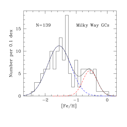
Figure 22.— Metallicity distribution function for the GCs in the Milky Way. The MP (blue dashed line) and MR (red dashed line) component solutions are shown in the figure and listed in the text.

References

- Alamo-Martínez et al. (2013) Alamo-Martínez, K. A., Blakeslee, J. P., Jee, M. J., Côté, P., Ferrarese, L., González-Lópezlira, R. A., Jordán, A., Meurer, G. R., Peng, E. W., & West, M. J. 2013, ApJ, 775, 20
- Ashman & Zepf (1992) Ashman, K. M. & Zepf, S. E. 1992, ApJ, 384, 50
- Bailin & Harris (2009) Bailin, J. & Harris, W. E. 2009, ApJ, 695, 1082
- Barker et al. (2004) Barker, M. K., Sarajedini, A., & Harris, J. 2004, ApJ, 606, 869
- Barmby et al. (2000) Barmby, P., Huchra, J. P., Brodie, J. P., Forbes, D. A., Schroder, L. L., & Grillmair, C. J. 2000, AJ, 119, 727
- Bassino et al. (2006) Bassino, L. P., Faifer, F. R., Forte, J. C., Dirsch, B., Richtler, T., Geisler, D., & Schuberth, Y. 2006, A&A, 451, 789
- Bassino et al. (2008) Bassino, L. P., Richtler, T., & Dirsch, B. 2008, MNRAS, 386, 1145
- Beasley et al. (2002) Beasley, M. A., Baugh, C. M., Forbes, D. A., Sharples, R. M., & Frenk, C. S. 2002, MNRAS, 333, 383
- Bellini et al. (2009) Bellini, A., Piotto, G., Bedin, L. R., King, I. R., Anderson, J., Milone, A. P., & Momany, Y. 2009, A&A, 507, 1393
- Bender et al. (1988) Bender, R., Doebereiner, S., & Moellenhoff, C. 1988, A&AS, 74, 385
- Bender et al. (2015) Bender, R., Kormendy, J., Cornell, M. E., & Fisher, D. B. 2015, ApJ, 807, 56 (B15)
- Bertin & Arnouts (1996) Bertin, E. & Arnouts, S. 1996, A&AS, 117, 393
- Blakeslee et al. (2010) Blakeslee, J. P., Cantiello, M., & Peng, E. W. 2010, ApJ, 710, 51
- Blakeslee et al. (1997) Blakeslee, J. P., Tonry, J. L., & Metzger, M. R. 1997, AJ, 114, 482
- Bridges et al. (1996) Bridges, T. J., Carter, D., Harris, W. E., & Pritchet, C. J. 1996, MNRAS, 281, 1290
- Brodie et al. (2014) Brodie, J. P., Romanowsky, A. J., Strader, J., Forbes, D. A., Foster, C., Jennings, Z. G., Pastorello, N., Pota, V., Usher, C., Blom, C., Kader, J., Roediger, J. C., Spitler, L. R., Villaume, A., Arnold, J. A., Kartha, S. S., & Woodley, K. A. 2014, ApJ, 796, 52
- Brodie & Strader (2006) Brodie, J. P. & Strader, J. 2006, ARA&A, 44, 193
- Caon et al. (1993) Caon, N., Capaccioli, M., & D’Onofrio, M. 1993, MNRAS, 265, 1013
- Carter (1978) Carter, D. 1978, MNRAS, 182, 797
- Cockcroft et al. (2009) Cockcroft, R., Harris, W. E., Wehner, E. M. H., Whitmore, B. C., & Rothberg, B. 2009, AJ, 138, 758
- Côté et al. (1998) Côté, P., Marzke, R. O., & West, M. J. 1998, ApJ, 501, 554
- Dirsch et al. (2003) Dirsch, B., Richtler, T., Geisler, D., Forte, J. C., Bassino, L. P., & Gieren, W. P. 2003, AJ, 125, 1908
- Durrell et al. (2014) Durrell, P. R., Côté, P., Peng, E. W., Blakeslee, J. P., Ferrarese, L., Mihos, J. C., Puzia, T. H., Lançon, A., Liu, C., Zhang, H., Cuillandre, J.-C., McConnachie, A., Jordán, A., Accetta, K., Boissier, S., Boselli, A., Courteau, S., Duc, P.-A., Emsellem, E., Gwyn, S., Mei, S., & Taylor, J. E. 2014, ApJ, 794, 103
- Fensch et al. (2014) Fensch, J., Mieske, S., Müller-Seidlitz, J., & Hilker, M. 2014, A&A, 567, A105
- Fleming et al. (1995) Fleming, D. E. B., Harris, W. E., Pritchet, C. J., & Hanes, D. A. 1995, AJ, 109, 1044
- Forbes et al. (1997) Forbes, D. A., Brodie, J. P., & Grillmair, C. J. 1997, AJ, 113, 1652
- Forbes et al. (2006) Forbes, D. A., Sánchez-Blázquez, P., Phan, A. T. T., Brodie, J. P., Strader, J., & Spitler, L. 2006, MNRAS, 366, 1230
- Forte et al. (2005) Forte, J. C., Faifer, F., & Geisler, D. 2005, MNRAS, 357, 56
- Forte et al. (2007) —. 2007, MNRAS, 382, 1947
- Forte et al. (2001) Forte, J. C., Geisler, D., Ostrov, P. G., Piatti, A. E., & Gieren, W. 2001, AJ, 121, 1992
- Forte et al. (2014) Forte, J. C., Vega, E. I., Faifer, F. R., Smith Castelli, A. V., Escudero, C., González, N. M., & Sesto, L. 2014, MNRAS, 441, 1391
- Gebhardt & Kissler-Patig (1999) Gebhardt, K. & Kissler-Patig, M. 1999, AJ, 118, 1526
- Geisler et al. (1996) Geisler, D., Lee, M. G., & Kim, E. 1996, AJ, 111, 1529
- Girardi et al. (2005) Girardi, L., Groenewegen, M. A. T., Hatziminaoglou, E., & da Costa, L. 2005, A&A, 436, 895
- Graham & Driver (2005) Graham, A. W. & Driver, S. P. 2005, PASA, 22, 118
- Griffen et al. (2010) Griffen, B. F., Drinkwater, M. J., Thomas, P. A., Helly, J. C., & Pimbblet, K. A. 2010, MNRAS, 405, 375
- Hargis & Rhode (2014) Hargis, J. R. & Rhode, K. L. 2014, ApJ, 796, 62
- Harris (1996) Harris, W. E. 1996, AJ, 112, 1487
- Harris (2009a) —. 2009a, ApJ, 699, 254
- Harris (2009b) —. 2009b, ApJ, 703, 939
- Harris & Harris (2002) Harris, W. E. & Harris, G. L. H. 2002, AJ, 123, 3108
- Harris et al. (2007) Harris, W. E., Harris, G. L. H., Layden, A. C., & Wehner, E. M. H. 2007, ApJ, 666, 903
- Harris et al. (2009) Harris, W. E., Kavelaars, J. J., Hanes, D. A., Pritchet, C. J., & Baum, W. A. 2009, AJ, 137, 3314
- Harris et al. (2014) Harris, W. E., Morningstar, W., Gnedin, O. Y., O’Halloran, H., Blakeslee, J. P., Whitmore, B. C., Côté, P., Geisler, D., Peng, E. W., Bailin, J., Rothberg, B., Cockcroft, R., & Barber DeGraaff, R. 2014, ApJ, 797, 128 (PaperI)
- Harris et al. (1995) Harris, W. E., Pritchet, C. J., & McClure, R. D. 1995, ApJ, 441, 120
- Harris & van den Bergh (1981) Harris, W. E. & van den Bergh, S. 1981, AJ, 86, 1627
- Harris et al. (2006) Harris, W. E., Whitmore, B. C., Karakla, D., Okoń, W., Baum, W. A., Hanes, D. A., & Kavelaars, J. J. 2006, ApJ, 636, 90
- Jordán et al. (2005) Jordán, A., Côté, P., Blakeslee, J. P., Ferrarese, L., McLaughlin, D. E., Mei, S., Peng, E. W., Tonry, J. L., Merritt, D., Milosavljević, M., Sarazin, C. L., Sivakoff, G. R., & West, M. J. 2005, ApJ, 634, 1002
- Kim et al. (2013) Kim, H.-S., Yoon, S.-J., Sohn, S. T., Kim, S. C., Kim, E., Chung, C., Lee, S.-Y., & Lee, Y.-W. 2013, ApJ, 763, 40
- Kravtsov & Gnedin (2005) Kravtsov, A. V. & Gnedin, O. Y. 2005, ApJ, 623, 650
- Kruijssen (2014) Kruijssen, J. M. D. 2014, Classical and Quantum Gravity, 31, 244006
- Kundu & Whitmore (2001) Kundu, A. & Whitmore, B. C. 2001, AJ, 121, 2950
- Larsen et al. (2001) Larsen, S. S., Brodie, J. P., Huchra, J. P., Forbes, D. A., & Grillmair, C. J. 2001, AJ, 121, 2974
- Lee et al. (2008) Lee, M. G., Park, H. S., Kim, E., Hwang, H. S., Kim, S. C., & Geisler, D. 2008, ApJ, 682, 135
- Li & Gnedin (2014) Li, H. & Gnedin, O. Y. 2014, ApJ, 796, 10
- McLaughlin et al. (1994) McLaughlin, D. E., Harris, W. E., & Hanes, D. A. 1994, ApJ, 422, 486
- McLaughlin & van der Marel (2005) McLaughlin, D. E. & van der Marel, R. P. 2005, ApJS, 161, 304
- Mieske et al. (2006) Mieske, S., Jordán, A., Côté, P., Kissler-Patig, M., Peng, E. W., Ferrarese, L., Blakeslee, J. P., Mei, S., Merritt, D., Tonry, J. L., & West, M. J. 2006, ApJ, 653, 193
- Mieske et al. (2010a) Mieske, S., Jordán, A., Côté, P., Peng, E. W., Ferrarese, L., Blakeslee, J. P., Mei, S., Baumgardt, H., Tonry, J. L., Infante, L., & West, M. J. 2010a, ApJ, 710, 1672
- Mieske et al. (2010b) —. 2010b, ApJ, 710, 1672
- Monachesi et al. (2015) Monachesi, A., Bell, E. F., Radburn-Smith, D., Bailin, J., de Jong, R. S., Holwerda, B., Streich, D., & Silverstein, G. 2015, MNRAS(submitted)
- Muratov & Gnedin (2010) Muratov, A. L. & Gnedin, O. Y. 2010, ApJ, 718, 1266
- Peacock et al. (2015) Peacock, M. B., Strader, J., Romanowsky, A. J., & Brodie, J. P. 2015, ApJ, 800, 13
- Peng et al. (2011) Peng, E. W., Ferguson, H. C., Goudfrooij, P., Hammer, D., Lucey, J. R., Marzke, R. O., Puzia, T. H., Carter, D., Balcells, M., Bridges, T., Chiboucas, K., del Burgo, C., Graham, A. W., Guzmán, R., Hudson, M. J., Matković, A., Merritt, D., Miller, B. W., Mouhcine, M., Phillipps, S., Sharples, R., Smith, R. J., Tully, B., & Verdoes Kleijn, G. 2011, ApJ, 730, 23
- Peng et al. (2009) Peng, E. W., Jordán, A., Blakeslee, J. P., Mieske, S., Côté, P., Ferrarese, L., Harris, W. E., Madrid, J. P., & Meurer, G. R. 2009, ApJ, 703, 42
- Peng et al. (2006) Peng, E. W., Jordán, A., Côté, P., Blakeslee, J. P., Ferrarese, L., Mei, S., West, M. J., Merritt, D., Milosavljević, M., & Tonry, J. L. 2006, ApJ, 639, 95
- Pritchet & Harris (1990) Pritchet, C. J. & Harris, W. E. 1990, ApJ, 355, 410
- Puzia et al. (1999) Puzia, T. H., Kissler-Patig, M., Brodie, J. P., & Huchra, J. P. 1999, AJ, 118, 2734
- Rhode & Zepf (2004) Rhode, K. L. & Zepf, S. E. 2004, AJ, 127, 302
- Saha et al. (2011) Saha, A., Shaw, R. A., Claver, J. A., & Dolphin, A. E. 2011, PASP, 123, 481
- Sersic (1968) Sersic, J. L. 1968, Atlas de galaxias australes
- Stetson (1987) Stetson, P. B. 1987, PASP, 99, 191
- Strader et al. (2006) Strader, J., Brodie, J. P., Spitler, L., & Beasley, M. A. 2006, AJ, 132, 2333
- Tonini (2013) Tonini, C. 2013, ApJ, 762, 39
- Usher et al. (2015) Usher, C., Forbes, D. A., Brodie, J. P., Romanowsky, A. J., Strader, J., Conroy, C., Foster, C., Pastorello, N., Pota, V., & Arnold, J. A. 2015, MNRAS, 446, 369
- Usher et al. (2013) Usher, C., Forbes, D. A., Spitler, L. R., Brodie, J. P., Romanowsky, A. J., Strader, J., & Woodley, K. A. 2013, MNRAS, 436, 1172