Exact Zero Vacuum Energy in twisted $SU(N)$ Principal Chiral Field

Sรฉbastien Leurenta, Evgeny Sobkob a Universitรฉ de Bourgogne Franche-Comtรฉ โ€“ Institut de Mathรฉmatiques de Bourgogne
UMR 5584 du CNRS, 9 avenue Alain Savary 21000 Dijon
b DESY Hamburg, Theory Group, NotkestraรŸe 85, 22607 Hamburg, Germany
Abstract

We present a finite set of equations for twisted PCF model. At the special twist in the root of unity we demonstrate that the vacuum energy is exactly zero at any size $L$. Also in $SU(2)$ case we numerically calculate the energy of the single particle state with zero rapidity, as a function of $L$.

โ€ โ€ preprint:

I Introduction

$SU(N)$ Principal Chiral Field on a cylinder of circumference $L$ has the following classical action $S$:

S=12โ€‹g2โ€‹โˆซโˆ’โˆžโˆž๐‘‘tโ€‹โˆซ0L๐‘‘xโ€‹trโ€‹โˆ‚ฮผUโ€‹โˆ‚ฮผUโ€ .๐‘†12superscript๐‘”2superscriptsubscriptdifferential-d๐‘กsuperscriptsubscript0๐ฟdifferential-d๐‘ฅtrsubscript๐œ‡๐‘ˆsuperscript๐œ‡superscript๐‘ˆโ€ \displaystyle S=\frac{1}{2g^{2}}\int\limits_{-\infty}^{\infty}dt\int\limits_{0}^{L}dx\ \text{tr}\ \partial_{\mu}U\partial^{\mu}U^{\dagger}. (1)

On the quantum level at $L\rightarrow\infty$ the theory with periodic boundary conditions has $N-1$ types of massive excitations which are in one to one correspondence with fundamental representations of $SU(N)$. The lowest mass $m=m_{1}$ is defined by the mechanism of dimensional transmutation $m=m_{1}=\frac{\Lambda}{g}e^{-\frac{4\pi}{Ng^{2}}}$. All other particles appear as bound states and have masses $m_{k}=m\frac{\sin(\frac{\pi k}{N})}{\sin(\frac{\pi}{N})}$. The spectrum of the theory on $\mathbb{R}^{2}$ can be completely solved by Bethe Ansatz technique Wiegmann:1984pw ; Ogievetsky:1987vv . In case of finite $L$ and periodic boundary conditions the finite system of integral equations with solution in terms of Wronskian determinants was presented in Kazakov:2010kf .

In this paper we generalize the construction of Kazakov:2010kf to the case of twisted boundary conditions $U(t,x+L)=e^{i\Phi}U(t,x)e^{-i\Phi}$. In the case of particular twist $e^{i\Phi}=\Omega=e^{i\frac{\pi}{N}\frac{1+(-1)^{N}}{2}}\text{diag}[1,e^{\frac{2\pi i}{N}},e^{\frac{4\pi i}{N}},...,e^{\frac{2\pi(N-1)i}{N}}]$ we calculate the energy of single particle state in the rest as a function of $L$ numerically and show that the vacuum energy is exactly zero. This zero is quite unexpected because PCF is a pure bosonic theory without SUSY.

II Twisted TBA

Using the usual logic of the derivation of TBA we can write the vacuum energy as

$$\displaystyle E_{0}^{d}=-\lim\limits_{R\rightarrow\infty}\frac{\log\text{tr}(e^{-H(L)R})}{R}$$ (2)

and then go to the mirror model $\text{Tr}(e^{-\tilde{H}(R)L})=\text{Tr}(e^{-H(L)R})$ with mirror Hamiltonian $\tilde{H}(R)$ and periodic boundary conditions. Twisted boundary conditions $U(t,x+L)=e^{i\Phi}U(t,x)e^{-i\Phi}$ in the original model can be formalized as an insertion of the defect operator in the mirror model Ahn:2011xq :

$$\displaystyle Tr(e^{-\tilde{H}(R)L}e^{i\mathbf{\Phi}})$$ (3)

where twist $e^{i\mathbf{\Phi}}$ commutes with the scattering matrix and acts on one particle states as $e^{i\Phi\otimes 1-1\otimes i\Phi}$ where $e^{i\Phi}=\text{diag}[e^{i\phi_{1}},e^{i\phi_{2}},...,e^{i\phi_{N}}]$. This twist leads us to the following TBA equations ($a\in[1,...,N-1]$):

$$\displaystyle\mu^{a,0}=mL\frac{\sin\frac{\pi a}{N}}{\sin\frac{\pi}{N}}\cosh\frac{2\pi}{N}u-\log\frac{1}{Y^{a,0}}+$$
$$\displaystyle+\sum\limits_{a^{\prime}}\mathcal{K}^{(a^{\prime},0),(a,0)}\ast\log(1+Y^{a^{\prime},0})+$$
โˆ‘sโ€ฒโ‰ 0,aโ€ฒ๐’ฆ(aโ€ฒ,sโ€ฒ),(a,0)โˆ—logโก(1+1Yaโ€ฒ,sโ€ฒ),subscriptsuperscript๐‘ โ€ฒ0superscript๐‘Žโ€ฒโˆ—superscript๐’ฆsuperscript๐‘Žโ€ฒsuperscript๐‘ โ€ฒ๐‘Ž011superscript๐‘Œsuperscript๐‘Žโ€ฒsuperscript๐‘ โ€ฒ\displaystyle\sum\limits_{s^{\prime}\neq 0,a^{\prime}}\mathcal{K}^{(a^{\prime},s^{\prime}),(a,0)}\ast\log(1+\frac{1}{Y^{a^{\prime},s^{\prime}}}),
ฮผa,sโ‰ 0=โˆ’logโกYa,s+โˆ‘aโ€ฒ๐’ฆ(aโ€ฒ,0),(a,s)โˆ—logโก(1+Yaโ€ฒ,0)+superscript๐œ‡๐‘Ž๐‘ 0superscript๐‘Œ๐‘Ž๐‘ limit-fromsubscriptsuperscript๐‘Žโ€ฒโˆ—superscript๐’ฆsuperscript๐‘Žโ€ฒ0๐‘Ž๐‘ 1superscript๐‘Œsuperscript๐‘Žโ€ฒ0\displaystyle\mu^{a,s\neq 0}=-\log Y^{a,s}+\sum\limits_{a^{\prime}}\mathcal{K}^{(a^{\prime},0),(a,s)}\ast\log(1+Y^{a^{\prime},0})+
โˆ‘sโ€ฒโ‰ 0,aโ€ฒ๐’ฆ(aโ€ฒ,sโ€ฒ),(a,s)โˆ—logโก(1+1Yaโ€ฒ,sโ€ฒ)subscriptsuperscript๐‘ โ€ฒ0superscript๐‘Žโ€ฒโˆ—superscript๐’ฆsuperscript๐‘Žโ€ฒsuperscript๐‘ โ€ฒ๐‘Ž๐‘ 11superscript๐‘Œsuperscript๐‘Žโ€ฒsuperscript๐‘ โ€ฒ\displaystyle\sum\limits_{s^{\prime}\neq 0,a^{\prime}}\mathcal{K}^{(a^{\prime},s^{\prime}),(a,s)}\ast\log(1+\frac{1}{Y^{a^{\prime},s^{\prime}}}) (4)

with chemical potentials ฮผa,ssuperscript๐œ‡๐‘Ž๐‘ \mu^{a,s}:

{ฮผa,s=โˆ’iโ€‹sโ€‹(ฯ•a+1โˆ’ฯ•a),s>0ฮผa,s=iโ€‹|s|โ€‹(ฯ•a+1โˆ’ฯ•a),s<0ฮผa,s=0,s=0casessubscript๐œ‡๐‘Ž๐‘ ๐‘–๐‘ subscriptitalic-ฯ•๐‘Ž1subscriptitalic-ฯ•๐‘Ž๐‘ 0subscript๐œ‡๐‘Ž๐‘ ๐‘–๐‘ subscriptitalic-ฯ•๐‘Ž1subscriptitalic-ฯ•๐‘Ž๐‘ 0subscript๐œ‡๐‘Ž๐‘ 0๐‘ 0\displaystyle\begin{cases}\mu_{a,s}=-is(\phi_{a+1}-\phi_{a}),&s>0\\ \mu_{a,s}=i|s|(\phi_{a+1}-\phi_{a}),&s<0\\ \mu_{a,s}=0,&s=0\end{cases} (5)

and all other ingredients are as in the untwisted case: kernels $\mathcal{K}$ are derivatives of logarithm of S-matrix which can be read off from Ogievetsky:1987vv and Y-functions $Y^{a,0}=\frac{\rho^{a,0}}{\bar{\rho}^{a,0}}$, Ya,sโ‰ 0=ฯยฏa,sฯa,ssuperscript๐‘Œ๐‘Ž๐‘ 0superscriptยฏ๐œŒ๐‘Ž๐‘ superscript๐œŒ๐‘Ž๐‘ Y^{a,s\neq 0}=\frac{\bar{\rho}^{a,s}}{\rho^{a,s}} are expressed through the hole and particleโ€™s densities ฯยฏa,ssuperscriptยฏ๐œŒ๐‘Ž๐‘ \bar{\rho}^{a,s}, ฯa,ssuperscript๐œŒ๐‘Ž๐‘ \rho^{a,s}. The convolution $\ast$ is defined in the usual way: $[f\ast g](u)=\int\limits_{-\infty}^{\infty}dvf(u-v)g(v)$. In terms of Y-functions TBA (4) can be rewritten as a usual Y-system:

Ya,s+โ€‹Ya,sโˆ’Ya,s+1โ€‹Ya,sโˆ’1=1+1/Ya,s+11+1/Ya+1,sโ€‹1+1/Ya,sโˆ’11+1/Yaโˆ’1,ssuperscriptsubscript๐‘Œ๐‘Ž๐‘ superscriptsubscript๐‘Œ๐‘Ž๐‘ subscript๐‘Œ๐‘Ž๐‘ 1subscript๐‘Œ๐‘Ž๐‘ 111subscript๐‘Œ๐‘Ž๐‘ 111subscript๐‘Œ๐‘Ž1๐‘ 11subscript๐‘Œ๐‘Ž๐‘ 111subscript๐‘Œ๐‘Ž1๐‘ \displaystyle\frac{Y_{a,s}^{+}Y_{a,s}^{-}}{Y_{a,s+1}Y_{a,s-1}}=\frac{1+1/Y_{a,s+1}}{1+1/Y_{a+1,s}}\frac{1+1/Y_{a,s-1}}{1+1/Y_{a-1,s}} (6)

At large $L$ all middle-node Y-functions are exponentially small Ya,0=cโ€‹oโ€‹nโ€‹sโ€‹tร—eโˆ’Lโ€‹pasubscript๐‘Œ๐‘Ž0๐‘๐‘œ๐‘›๐‘ ๐‘กsuperscript๐‘’๐ฟsubscript๐‘๐‘ŽY_{a,0}=const\times e^{-Lp_{a}} and Y-system splits in two independent left and right wings. Here we have introduced the momentum of aโ€™s particle $p_{a}(\theta)=m\frac{\sin\frac{a\pi}{N}}{\sin\frac{\pi}{N}}\cosh\frac{2\pi}{N}\theta$ The asymptotic solution at $L\rightarrow\infty$ can be written as:

Ya,s=ฯ‡a,s+1โ€‹(eโˆ’iโ€‹ฮฆ)โ€‹ฯ‡a,sโˆ’1โ€‹(eโˆ’iโ€‹ฮฆ)ฯ‡a+1,sโ€‹(eโˆ’iโ€‹ฮฆ)โ€‹ฯ‡aโˆ’1,sโ€‹(eโˆ’iโ€‹ฮฆ),s>0formulae-sequencesubscript๐‘Œ๐‘Ž๐‘ subscript๐œ’๐‘Ž๐‘ 1superscript๐‘’๐‘–ฮฆsubscript๐œ’๐‘Ž๐‘ 1superscript๐‘’๐‘–ฮฆsubscript๐œ’๐‘Ž1๐‘ superscript๐‘’๐‘–ฮฆsubscript๐œ’๐‘Ž1๐‘ superscript๐‘’๐‘–ฮฆ๐‘ 0\displaystyle Y_{a,s}=\frac{\chi_{a,s+1}(e^{-i\Phi})\chi_{a,s-1}(e^{-i\Phi})}{\chi_{a+1,s}(e^{-i\Phi})\chi_{a-1,s}(e^{-i\Phi})},\ \ \ s>0
Ya,0=ฯ‡a,1โ€‹(eiโ€‹ฮฆ)โ€‹ฯ‡a,1โ€‹(eโˆ’iโ€‹ฮฆ)โ€‹eโˆ’Lโ€‹paโ€‹(u),s=0formulae-sequencesubscript๐‘Œ๐‘Ž0subscript๐œ’๐‘Ž1superscript๐‘’๐‘–ฮฆsubscript๐œ’๐‘Ž1superscript๐‘’๐‘–ฮฆsuperscript๐‘’๐ฟsubscript๐‘๐‘Ž๐‘ข๐‘ 0\displaystyle Y_{a,0}=\chi_{a,1}(e^{i\Phi})\chi_{a,1}(e^{-i\Phi})e^{-Lp_{a}(u)},\ \ \ s=0
Ya,s=ฯ‡a,|s|+1โ€‹(eiโ€‹ฮฆ)โ€‹ฯ‡a,|s|โˆ’1โ€‹(eiโ€‹ฮฆ)ฯ‡a+1,|s|โ€‹(eiโ€‹ฮฆ)โ€‹ฯ‡aโˆ’1,|s|โ€‹(eiโ€‹ฮฆ),s<0formulae-sequencesubscript๐‘Œ๐‘Ž๐‘ subscript๐œ’๐‘Ž๐‘ 1superscript๐‘’๐‘–ฮฆsubscript๐œ’๐‘Ž๐‘ 1superscript๐‘’๐‘–ฮฆsubscript๐œ’๐‘Ž1๐‘ superscript๐‘’๐‘–ฮฆsubscript๐œ’๐‘Ž1๐‘ superscript๐‘’๐‘–ฮฆ๐‘ 0\displaystyle Y_{a,s}=\frac{\chi_{a,|s|+1}(e^{i\Phi})\chi_{a,|s|-1}(e^{i\Phi})}{\chi_{a+1,|s|}(e^{i\Phi})\chi_{a-1,|s|}(e^{i\Phi})},\ \ \ s<0 (7)

where ฯ‡a,sโ€‹(g)subscript๐œ’๐‘Ž๐‘ ๐‘”\chi_{a,s}(g) is a character of $g$ in the representation with rectangular Young tableau with $a$ rows and s๐‘ s columns. The ansatz (7) obviously solves Y-system (6) up to $O(e^{-mL})$ terms. However Y-system (6) doesnโ€™t depend on twist and we have to check that solution (7) goes through TBA (4) and reproduces the right chemical potentials. Turn out that a special regularization is needed. Namely we should formally modify the twist as

$$\displaystyle e^{\pm i\Phi}\rightarrow\text{diag}\{e^{\pm i\phi_{1}}e^{\epsilon_{1}},e^{\pm i\phi_{2}}e^{\epsilon_{2}},...,e^{\pm i\phi_{N}}e^{\epsilon_{N}}\}$$ (8)

where $0>\epsilon_{1}>\epsilon_{2}>...>\epsilon_{N}$, $\frac{\epsilon_{i}}{\epsilon_{i+1}}$ - fixed and $\epsilon_{N}\rightarrow 0$. Letโ€™s show how this prescription reproduces the chemical potentials in the case of $a\in[2,...,N-2]$ and s>0๐‘ 0s>0. The corresponding equation reads:

ฮผa,s=โˆ’logโก(Ya,s)โˆ’โˆ‘sโ€ฒ=1โˆžmโ€‹iโ€‹nโ€‹(s,sโ€ฒ)โ€‹logโก(1+1Yaโˆ’1,sโ€ฒ)+subscript๐œ‡๐‘Ž๐‘ subscript๐‘Œ๐‘Ž๐‘ limit-fromsuperscriptsubscriptsuperscript๐‘ โ€ฒ1๐‘š๐‘–๐‘›๐‘ superscript๐‘ โ€ฒ11subscript๐‘Œ๐‘Ž1superscript๐‘ โ€ฒ\displaystyle\mu_{a,s}=-\log(Y_{a,s})-\sum\limits_{s^{\prime}=1}^{\infty}min(s,s^{\prime})\log(1+\frac{1}{Y_{a-1,s^{\prime}}})+
+โˆ‘sโ€ฒ=1โˆž(2โ€‹mโ€‹iโ€‹nโ€‹(s,sโ€ฒ)โˆ’ฮดs,sโ€ฒ)โ€‹logโก(1+1Ya,sโ€ฒ)โˆ’limit-fromsuperscriptsubscriptsuperscript๐‘ โ€ฒ12๐‘š๐‘–๐‘›๐‘ superscript๐‘ โ€ฒsubscript๐›ฟ๐‘ superscript๐‘ โ€ฒ11subscript๐‘Œ๐‘Žsuperscript๐‘ โ€ฒ\displaystyle+\sum\limits_{s^{\prime}=1}^{\infty}(2min(s,s^{\prime})-\delta_{s,s^{\prime}})\log(1+\frac{1}{Y_{a,s^{\prime}}})-
โˆ’โˆ‘sโ€ฒ=1โˆžmโ€‹iโ€‹nโ€‹(s,sโ€ฒ)โ€‹logโก(1+1Ya+1,sโ€ฒ)+Oโ€‹(eโˆ’mโ€‹L)superscriptsubscriptsuperscript๐‘ โ€ฒ1๐‘š๐‘–๐‘›๐‘ superscript๐‘ โ€ฒ11subscript๐‘Œ๐‘Ž1superscript๐‘ โ€ฒ๐‘‚superscript๐‘’๐‘š๐ฟ\displaystyle-\sum\limits_{s^{\prime}=1}^{\infty}min(s,s^{\prime})\log(1+\frac{1}{Y_{a+1,s^{\prime}}})+O(e^{-mL}) (9)

Now letโ€™s exponentiate its right hand side:

er.h.s. of (9)=superscript๐‘’r.h.s. of (9)absent\displaystyle e^{\text{r.h.s. of (\ref{a2N-2sneq0})}}=
=limpโ†’โˆž(ฯ‡aโˆ’1,p+1โ€‹(eiโ€‹ฮฆ)ฯ‡aโˆ’1,pโ€‹(eiโ€‹ฮฆ)โ€‹ฯ‡a,pโ€‹(eiโ€‹ฮฆ)2ฯ‡a,p+1โ€‹(eiโ€‹ฮฆ)2โ€‹ฯ‡a+1,p+1โ€‹(eiโ€‹ฮฆ)ฯ‡a+1,pโ€‹(eiโ€‹ฮฆ))sabsentsubscriptโ†’๐‘superscriptsubscript๐œ’๐‘Ž1๐‘1superscript๐‘’๐‘–ฮฆsubscript๐œ’๐‘Ž1๐‘superscript๐‘’๐‘–ฮฆsubscript๐œ’๐‘Ž๐‘superscriptsuperscript๐‘’๐‘–ฮฆ2subscript๐œ’๐‘Ž๐‘1superscriptsuperscript๐‘’๐‘–ฮฆ2subscript๐œ’๐‘Ž1๐‘1superscript๐‘’๐‘–ฮฆsubscript๐œ’๐‘Ž1๐‘superscript๐‘’๐‘–ฮฆ๐‘ \displaystyle=\lim\limits_{p\rightarrow\infty}\left(\frac{\chi_{a-1,p+1}(e^{i\Phi})}{\chi_{a-1,p}(e^{i\Phi})}\frac{\chi_{a,p}(e^{i\Phi})^{2}}{\chi_{a,p+1}(e^{i\Phi})^{2}}\frac{\chi_{a+1,p+1}(e^{i\Phi})}{\chi_{a+1,p}(e^{i\Phi})}\right)^{s} (10)

Using the above-mentioned epsilon-prescription and the first Weyl formula for characters itโ€™s easy to verify that:

$$\displaystyle\lim\limits_{p\rightarrow\infty}\frac{\chi_{a,p+1}}{\chi_{a,p}}=e^{-i\phi_{1}}e^{-i\phi_{2}}...e^{-i\phi_{a}}$$ (11)

what gives us exponent of l.h.s. of (9):

er.h.s. of (9)=(eโˆ’iโ€‹ฯ•a+1eโˆ’iโ€‹ฯ•a)s=eฮผa,ssuperscript๐‘’r.h.s. of (9)superscriptsuperscript๐‘’๐‘–subscriptitalic-ฯ•๐‘Ž1superscript๐‘’๐‘–subscriptitalic-ฯ•๐‘Ž๐‘ superscript๐‘’subscript๐œ‡๐‘Ž๐‘ \displaystyle e^{\text{r.h.s. of (\ref{a2N-2sneq0})}}=\left(\frac{e^{-i\phi_{a+1}}}{e^{-i\phi_{a}}}\right)^{s}=e^{\mu_{a,s}} (12)

For other values of $a$ and s๐‘ s the consideration is similar.

III Exact solution for vacuum at twist $\Omega$

It is surprising that the asymptotic solution (7) turns out to be exact at the twist $\Omega$. Indeed in case of large $L$ middle-node Y-functions $Y_{a,0}$ was exponentially small, leading to the decoupling of left and right wings. At the twist $\Omega$ all characters in fundamental representations are zero $\chi_{a,0}(\Omega)=0$ and it leads to a vanishing middle-node Y-functions $Y_{a,0}=0$. This formal solution is singular but it has a natural regularization with above-mentioned epsilon-prescription. In the case of $\epsilon_{i}\rightarrow 0$ the ansatz (7) solves Y-system (or TBA) up to the terms $o(\epsilon)$ and gives us solution at any $L$. Due to the vacuum energy formula:

$$\displaystyle E_{\Omega}^{exact}(L)=$$
$$\displaystyle=\lim\limits_{\epsilon_{i}\rightarrow 0}-\frac{1}{N}\sum\limits_{a=1}^{N-1}\int\limits_{-\infty}^{\infty}d\theta p_{a}(\theta)\log(1+o(\epsilon_{i}))=0$$ (13)

we get exact zero for vacuum energy.

At the large $L$ limit this zero energy can be seen directly from (3). Indeed the leading contribution is a sum over one-particle states and for the particle of the type $a$ we get factor $\chi_{a,0}(e^{i\Phi})\chi_{a,0}(e^{-i\Phi})$ which comes from the sum over basis vectors of fundamental representation with $a$ vertical boxes:

$$\displaystyle\sum\limits_{p}\langle p|e^{i\mathbf{\Phi}}|p\rangle=\chi_{a,0}(e^{i\Phi})\chi_{a,0}(e^{-i\Phi})$$ (14)

what gives zero at twist $\Omega$. The next correction is a Lรผscher term corresponding to two-particle contribution and in the $SU(2)$ case it was calculated in Ahn:2011xq . Plugging the twist $\Omega$ in (3.43) of Ahn:2011xq it is easy to verify that the Lรผscher term vanishes.

On the other hand, at small $L$, we have a weakly coupled theory and the one-loop Casimir energy was presented 111At the presence of fermions with $N_{f}$ flavors formula (15) modifies Cherman:2014ofa as $E_{e^{i\mathbf{\Phi}}}^{1-loop}=-(N_{f}-1)\frac{1}{\pi L}\sum\limits_{n=1}^{\infty}\frac{1}{n^{2}}\left(\left|tr(e^{in\Phi})\right|^{2}-1\right)$. At $N_{f}=1$ the theory has $(1,1)$ supersymmetry and the theory has zero vacuum energy. in Cherman:2014ofa :

$$\displaystyle E_{e^{i\mathbf{\Phi}}}^{1-loop}=-\frac{1}{\pi L}\sum\limits_{n=1}^{\infty}\frac{1}{n^{2}}\left(\left|tr(e^{in\Phi})\right|^{2}-1\right)$$ (15)

In the periodic case we have the standard Casimir energy

$$\displaystyle E_{periodic}^{1-loop}=-\frac{1}{\pi L}\sum\limits_{n=1}^{\infty}\frac{1}{n^{2}}(N^{2}-1)=-\frac{\pi(N^{2}-1)}{6L},$$

corresponding to $N^{2}-1$ free bosons Kazakov:2010kf .

In the case of twist $\Omega$ we have:

$$\displaystyle E_{\Omega}^{1-loop}=-\frac{1}{\pi L}\left(\sum\limits_{k=1}^{\infty}\frac{1}{(Nk)^{2}}(N)^{2}-\sum\limits_{n=1}^{\infty}\frac{1}{n^{2}}\right)=0,$$ (16)

because $\text{tr}\ \Omega^{n}=0$ for nโ‰ Nโ€‹k๐‘›๐‘๐‘˜n\neq Nk

IV ABA

The Y-system (6) can be reformulated in the form of Hirota equations:

Ta,s+โ€‹Ta,sโˆ’=Ta+1,sโ€‹Taโˆ’1,s+Ta,s+1โ€‹Ta,sโˆ’1subscriptsuperscript๐‘‡๐‘Ž๐‘ subscriptsuperscript๐‘‡๐‘Ž๐‘ subscript๐‘‡๐‘Ž1๐‘ subscript๐‘‡๐‘Ž1๐‘ subscript๐‘‡๐‘Ž๐‘ 1subscript๐‘‡๐‘Ž๐‘ 1\displaystyle T^{+}_{a,s}T^{-}_{a,s}=T_{a+1,s}T_{a-1,s}+T_{a,s+1}T_{a,s-1} (17)

and the original Y-functions are expressed through the set of {Ta,sโ€‹(ฮธ)}subscript๐‘‡๐‘Ž๐‘ ๐œƒ\{T_{a,s}(\theta)\} as Ya,s=Ta,s+1โ€‹Ta,sโˆ’1Ta+1,sโ€‹Taโˆ’1,ssubscript๐‘Œ๐‘Ž๐‘ subscript๐‘‡๐‘Ž๐‘ 1subscript๐‘‡๐‘Ž๐‘ 1subscript๐‘‡๐‘Ž1๐‘ subscript๐‘‡๐‘Ž1๐‘ Y_{a,s}=\frac{T_{a,s+1}T_{a,s-1}}{T_{a+1,s}T_{a-1,s}}.

In the presence of the twist $e^{i\mathbf{\Phi}}$ the general solution of Hirota equation (up to a gauge degrees of freedom) has the following generating functional for T-functions $\lim_{L\to\infty}T^{R}$:

$$\displaystyle\hat{W}^{R}=\frac{1}{(1-e^{-i\phi_{N}}X_{(N)}^{R}(\theta)e^{i\partial_{\theta}})}\cdot$$
$$\displaystyle\cdot\frac{1}{(1-e^{-i\phi_{N-1}}X_{(N-1)}^{R}(\theta)e^{i\partial_{\theta}})}\cdot...\cdot\frac{1}{(1-e^{-i\phi_{1}}X_{(1)}^{R}(\theta)e^{i\partial_{\theta}})}$$
=โˆ‘s=0โˆžT1,sRโ€‹(ฮธ+i2โ€‹(sโˆ’1))ฯ†โ€‹(ฮธโˆ’iโ€‹N4)โ€‹eiโ€‹sโ€‹โˆ‚ฮธ,absentsuperscriptsubscript๐‘ 0superscriptsubscript๐‘‡1๐‘ ๐‘…๐œƒ๐‘–2๐‘ 1๐œ‘๐œƒ๐‘–๐‘4superscript๐‘’๐‘–๐‘ subscript๐œƒ\displaystyle=\sum\limits_{s=0}^{\infty}\frac{T_{1,s}^{R}(\theta+\frac{i}{2}(s-1))}{\varphi(\theta-i\frac{N}{4})}e^{is\partial_{\theta}}, (18)

where $X_{k}^{R}$ and $\varphi(\theta)$ are defined as in Kazakov:2010kf , in terms of some polynomial functions $Q_{k}^{R}$ encoding the excitations defining a given state. The exponent $R$ stands for a specific choice of gauge where limLโ†’โˆžTa,sR=0subscriptโ†’๐ฟsuperscriptsubscript๐‘‡๐‘Ž๐‘ ๐‘…0\lim_{L\to\infty}T_{a,s}^{R}=0 is zero if s<0๐‘ 0s<0 with $0<a<N$, whereas for other values of (a,s)๐‘Ž๐‘ (a,s) the limit is a polynomial.

Similarly, there exists a gauge denoted $T^{L}$ where limLโ†’โˆžTa,sLsubscriptโ†’๐ฟsuperscriptsubscript๐‘‡๐‘Ž๐‘ ๐ฟ\lim_{L\to\infty}T_{a,s}^{L} vanishes if s>0๐‘ 0s>0 with $0<a<N$. T1,โˆ’sLsuperscriptsubscript๐‘‡1๐‘ ๐ฟT_{1,-s}^{L} has a generating series which differs from the generating series (18) of T1,sRsuperscriptsubscript๐‘‡1๐‘ ๐‘…T_{1,s}^{R} by the substitution $\phi_{i}\rightarrow-\phi_{i}$

Canceling poles at $T^{R}_{1,1}$ at $w-\frac{i}{2}(\frac{N}{2}-k+1)$ we get the twisted auxiliary Bethe equations:

$$\displaystyle-e^{i(\phi_{k-1}-\phi_{k})}=\frac{Q^{R}_{k-2}(w-\frac{i}{2})Q^{R}_{k-1}(w+i)Q^{R}_{k}(w-\frac{i}{2})}{Q^{R}_{k-2}(w+\frac{i}{2})Q^{R}_{k-1}(w-i)Q^{R}_{k}(w+\frac{i}{2})}$$ (19)

and similar for the left wing.

Asymptotic form of middle-node Y-functions reads as:

$$\displaystyle Y_{a,0}(\theta)\sim e^{-mLp_{a}}\frac{T_{a,1}T^{L}_{a,-1}}{T_{a+1,0}T_{a-1,0}}\frac{\varphi^{[-\frac{N}{2}-a+1]}\varphi^{[-\frac{N}{2}-a+1]}}{\varphi^{[-\frac{N}{2}+a-1]}\varphi^{[-\frac{N}{2}+a+1]}}\cdot$$
โ‹…1ฮ aโ€‹((S[โˆ’N2])2โ€‹ฯ‡Cโ€‹Dโ€‹D[โˆ’N2])โ‹…absent1subscriptฮ ๐‘Žsuperscriptsuperscript๐‘†delimited-[]๐‘22superscriptsubscript๐œ’๐ถ๐ท๐ทdelimited-[]๐‘2\displaystyle\cdot\frac{1}{\Pi_{a}\left((S^{[-\frac{N}{2}]})^{2}\chi_{CDD}^{[-\frac{N}{2}]}\right)} (20)

and it leads to the massive Bethe equation $Y_{1,0}(\theta_{j}+i\frac{N}{4})=0$ as in the untwisted case222explicit form of S-matrix $S$ and CDD factor $\chi_{CDD}$ can be found in Kazakov:2010kf :

$$\displaystyle-1=\frac{e^{-imL\sinh\frac{2\pi}{N}\theta_{j}}}{\chi_{CDD}S^{2}(\theta_{j})}\frac{Q^{R}_{N-1}(\theta_{j}-\frac{i}{2})Q^{L}_{N-1}(\theta_{j}-\frac{i}{2})}{Q^{R}_{N-1}(\theta_{j}+\frac{i}{2})Q^{L}_{N-1}(\theta_{j}+\frac{i}{2})}$$ (21)

V Finite L

Up to some gauge degrees of freedom, the general solution of Hirota equation can be represented through the following Wronskian determinant:

Ta,s(R)โ€‹(ฮธ)=iNโ€‹(Nโˆ’1)2โ€‹Detโ€‹(cj,k)1โฉฝj,kโฉฝNsuperscriptsubscript๐‘‡๐‘Ž๐‘ ๐‘…๐œƒsuperscript๐‘–๐‘๐‘12Detsubscriptsubscript๐‘๐‘—๐‘˜formulae-sequence1๐‘—๐‘˜๐‘\displaystyle T_{a,s}^{(R)}(\theta)=i^{\frac{N(N-1)}{2}}\mathrm{Det}(c_{j,k})_{1\leqslant j,k\leqslant N} (22)
whereย โ€‹cj,k={eiโ€‹ฯ•jโ€‹(s/2โˆ’k)โ€‹qjยฏ[s+a+1+N2โˆ’2โ€‹k]ifย โ€‹kโฉฝaeiโ€‹ฯ•jโ€‹(โˆ’s/2โˆ’k)โ€‹qj[โˆ’s+a+1+N2โˆ’2โ€‹k]ifย โ€‹k>a,whereย subscript๐‘๐‘—๐‘˜casessuperscript๐‘’๐‘–subscriptitalic-ฯ•๐‘—๐‘ 2๐‘˜superscriptยฏsubscript๐‘ž๐‘—delimited-[]๐‘ ๐‘Ž1๐‘22๐‘˜ifย ๐‘˜๐‘Žsuperscript๐‘’๐‘–subscriptitalic-ฯ•๐‘—๐‘ 2๐‘˜superscriptsubscript๐‘ž๐‘—delimited-[]๐‘ ๐‘Ž1๐‘22๐‘˜ifย ๐‘˜๐‘Ž\displaystyle\textrm{where }c_{j,k}=\begin{cases}e^{i\phi_{j}(s/2-k)}\overline{q_{j}}^{[s+a+1+\frac{N}{2}-2k]}&\textrm{if }k\leqslant a\\ e^{i\phi_{j}(-s/2-k)}q_{j}^{[-s+a+1+\frac{N}{2}-2k]}&\textrm{if }k>a\,,\end{cases}

in terms of $2\,N$ complex functions $\{q_{j}\,\bar{q}_{j}\}$, where we use the notation $f^{[n]}(\theta)\equiv f(\theta+n\tfrac{i}{2})$. It turns out Kazakov:2010kf that $q_{j}$ (resp $\bar{q}_{j}$) is analytic on the lower (resp upper) half plane, and that $q_{j}$ and $\bar{q}_{j}$ are complex conjugated, so that one has Ta,sโ€‹(ฮธ)ยฏ=TNโˆ’a,sโ€‹(ฮธยฏ)ยฏsubscript๐‘‡๐‘Ž๐‘ ๐œƒsubscript๐‘‡๐‘๐‘Ž๐‘ ยฏ๐œƒ\overline{T_{a,s}(\theta)}=T_{N-a,s}(\bar{\theta}). In addition $q_{j}-\bar{q}_{j}$ decreases at large $\theta$ as $e^{-L\cosh(2\pi/N\theta)}$, hence the parameterisation

$$P_{j}+i\,\mathcal{C}*f_{j}=\begin{cases}\bar{q}_{j}&\textrm{if }\mathrm{Im}(\theta)>0\\ q_{j}&\textrm{if }\mathrm{Im}(\theta)<0\end{cases}$$ (23)

where $\mathcal{C}\equiv\frac{1}{2i\pi\theta}$ is the Cauchy Kernel, $f_{j}\equiv i(\bar{q}_{j}-q_{j})$ is a real jump density and the $P_{j}$โ€™s are polynomial whose $L\to\infty$ limit is related (through Wronskian determinants) to the polynomials $Q_{j}^{R}$. In the periodic case, it was shown Kazakov:2010kf how to write equations for the densities $f_{j}$ for symmetric states, i.e. for states such that Ta,sR=Ta,โˆ’sLsuperscriptsubscript๐‘‡๐‘Ž๐‘ ๐‘…superscriptsubscript๐‘‡๐‘Ž๐‘ ๐ฟT_{a,s}^{R}=T_{a,-s}^{L}.

For the single particle state with zero rapidity, which we denote $\Theta_{0}$ and which defines the mass gap in the periodic case, this symmetry Ta,sR=Ta,โˆ’sLsuperscriptsubscript๐‘‡๐‘Ž๐‘ ๐‘…superscriptsubscript๐‘‡๐‘Ž๐‘ ๐ฟT_{a,s}^{R}=T_{a,-s}^{L} is actually broken by the introduction of the twist. One can however see that for several states such as the vacuum and this state $\Theta_{0}$, the introduction of the twist preserves a slightly different symmetry:

Ta,โˆ’s(L)โ€‹(ฮธ)=(โˆ’1)๐’ฉโ€‹TNโˆ’a,sโ€‹(โˆ’ฮธ)superscriptsubscript๐‘‡๐‘Ž๐‘ ๐ฟ๐œƒsuperscript1๐’ฉsubscript๐‘‡๐‘๐‘Ž๐‘ ๐œƒ{T_{a,-s}^{(L)}(\theta)=(-1)^{\mathcal{N}}T_{N-a,s}(-\theta)}\, (24)

where $\mathcal{N}$ denotes the number of Bethe roots (for instance it is zero for vacuum). One can easily follow the lines of Kazakov:2010kf to write equations for the densities of such state. In what follows we will do this for both the vacuum and the single-particle state $\Theta_{0}$, in the $N=2$ case.

For Vacuum we have $Q_{j}^{R}=1=Q_{j}^{L}$ (for all $j$), which corresponds to $P_{j}=1$ in (23). By contrast, the considered single-particle state $\Theta_{0}$ has $Q_{1}^{R}=Q_{1}^{L}=1$ and $Q_{2}^{R}(\theta)=Q_{2}^{L}(\theta)=\theta$, i.e. $P_{1}=1$ and $P_{2}(\theta)=\theta+c$ where $\lim_{mL\to\infty}c=-\frac{1}{2\tan\phi}$. Gauge freedom allows to set $q_{1}=1$, and then one can notice that $T_{1,-1}=-i(\bar{q}_{2}-q_{2})=-f_{2}$, hence the general expression (22) reduces to

T1,s(R)=iโ€‹eโˆ’iโ€‹(s+1)โ€‹ฯ•โ€‹((ฮธ[s+1]+c)๐’ฉ+iโ€‹๐’ž[s+1]โˆ—T1,โˆ’1(R))โˆ’iโ€‹eiโ€‹(s+1)โ€‹ฯ•โ€‹((ฮธ[โˆ’sโˆ’1]+c)๐’ฉ+iโ€‹๐’ž[โˆ’sโˆ’1]โˆ—T1,โˆ’1(R)),superscriptsubscript๐‘‡1๐‘ ๐‘…๐‘–superscript๐‘’๐‘–๐‘ 1italic-ฯ•superscriptsuperscript๐œƒdelimited-[]๐‘ 1๐‘๐’ฉ๐‘–superscript๐’ždelimited-[]๐‘ 1superscriptsubscript๐‘‡11๐‘…๐‘–superscript๐‘’๐‘–๐‘ 1italic-ฯ•superscriptsuperscript๐œƒdelimited-[]๐‘ 1๐‘๐’ฉ๐‘–superscript๐’ždelimited-[]๐‘ 1superscriptsubscript๐‘‡11๐‘…T_{1,s}^{(R)}=ie^{-i(s+1)\phi}\left((\theta^{[s+1]}+c)^{\mathcal{N}}+i\mathcal{C}^{[s+1]}*T_{1,-1}^{(R)}\right)\\ -ie^{i(s+1)\phi}\left((\theta^{[-s-1]}+c)^{\mathcal{N}}+i\mathcal{C}^{[-s-1]}*T_{1,-1}^{(R)}\right)\,, (25)

where the equation is valid for |Imโ€‹(ฮธ)|<s+1Im๐œƒ๐‘ 1|\mathrm{Im}(\theta)|<s+1, we denote $\phi\equiv\phi_{1}=-\phi_{2}$ and the single particle state $\Theta_{0}$ corresponds to $\mathcal{N}=1$ while the vacuum corresponds to $\mathcal{N}=0$.

If $\mathcal{N}=1$, the expression (25) involves a constant $c$ which is fixed at finite size by the condition $\left.T_{1,1}^{R}\right|_{\theta=0}=0$. This condition comes from the requirement that $T_{1,1}^{R}(\theta)$ and $T_{1,1}^{L}(\theta)=-T_{1,1}^{R}(-\theta)$ are gauge-equivalent, and if the gauge transformation is regular this means that the zeroes of $T_{1,1}^{R}$ are symmetric under $\theta\to-\theta$. Hence the zero which lies at origin in the $L\to\infty$ limit stays exactly at origin at finite $L$.

If we denote by T^ssubscript^๐‘‡๐‘ \hat{T}_{s} the function on the r.h.s. of (25), the equation (25) now reads: |Imโ€‹(ฮธ)|<s+1โ‡’T^sโ€‹(ฮธ)=T1,s(R)โ€‹(ฮธ)Im๐œƒ๐‘ 1โ‡’subscript^๐‘‡๐‘ ๐œƒsuperscriptsubscript๐‘‡1๐‘ ๐‘…๐œƒ|\mathrm{Im}(\theta)|<s+1\Rightarrow\hat{T}_{s}(\theta)=T_{1,s}^{(R)}(\theta). Then we can follow the lines of Gromov:2008gj to find integral equations for the function $T_{1,-1}^{(R)}$ entering equations (25) are obtained followingGromov:2008gj . First, one obtains

$\displaystyle\hat{T}_{0}(\theta)$ $\displaystyle=\begin{cases}T_{2,0}^{(R)}(\theta-\tfrac{i}{2})&\textrm{ if }\mathrm{Im}(\theta)>\tfrac{1}{2}\\ T_{1,0}^{(R)}(\theta)&\textrm{ if }\mathrm{Im}(\theta)\in]-\tfrac{1}{2},\tfrac{1}{2}[\\ T_{0,0}^{(R)}(\theta+\tfrac{i}{2})&\textrm{ if }\mathrm{Im}(\theta)<-\tfrac{1}{2}\,.\end{cases}$ (26)

Next, one gets (for $|\mathrm{Im}(\theta)|<1/2$)

$\displaystyle Y_{1,0}$ =eโˆ’mโ€‹Lโ€‹coshโก(ฯ€โ€‹ฮธ)โ€‹(โˆ’1)๐’ฉ+ฯƒโ€‹T^1โ€‹{T^1}(|T^0[+2]โ€‹{T^0[+2]}|2)โˆ—sabsentsuperscript๐‘’๐‘š๐ฟ๐œ‹๐œƒsuperscript1๐’ฉ๐œŽsubscript^๐‘‡1subscript^๐‘‡1superscriptsuperscriptsuperscriptsubscript^๐‘‡0delimited-[]2superscriptsubscript^๐‘‡0delimited-[]22absent๐‘ \displaystyle=e^{-mL\cosh(\pi\theta)}\frac{(-1)^{\mathcal{N}+\sigma}\hat{T}_{1}\{\hat{T}_{1}\}}{\left(|\hat{T}_{0}^{[+2]}\{\hat{T}_{0}^{[+2]}\}|^{2}\right)^{*s}} (27)

where we use the reality of $\hat{T}$ and we denote fโˆ—s=expโก(logโกfโˆ—(1/(2โ€‹coshโก(ฯ€โ€‹ฮธ))))superscript๐‘“absent๐‘ ๐‘“12๐œ‹๐œƒf^{*s}=\exp(\log f*(1/(2\cosh(\pi\theta)))).

The parameter $\sigma\in\{0,1\}$ is an a priori remaining freedom, from the fact that the equation for $Y_{1,0}^{+}Y_{1,0}^{-}$ only fixes $Y_{1,0}$ up to a sign. This sign can also be interpreted as an ambiguity in the choice of the branch of the log in fโˆ—s=eโ€‹xโ€‹pโ€‹(logโก(f)โˆ—s)superscript๐‘“absent๐‘ ๐‘’๐‘ฅ๐‘๐‘“๐‘ f^{*s}=exp(\log(f)*s). In the periodic case ($\phi=0$), this sign is $\sigma=0$ and it is fixed by requiring $Y_{1,0}$ to be a positive function. In our numeric resolution, we assumed that $\sigma=0$ holds also at arbitrary twist.

Finally, since we have on the real axis $Y_{1,0}=\frac{\hat{T}_{1}T_{1,-1}^{(R)}}{|\hat{T}_{0}^{[+1+0]}|^{2}}$, we get

T1,โˆ’1(R)=eโˆ’mโ€‹Lโ€‹coshโก(ฯ€โ€‹ฮธ)โ€‹(โˆ’1)๐’ฉ+ฯƒโ€‹|T^0[+1+0]|2โ€‹{T^1}(|T^0[+2]โ€‹{T^0[+2]}|2)โˆ—s.superscriptsubscript๐‘‡11๐‘…superscript๐‘’๐‘š๐ฟ๐œ‹๐œƒsuperscript1๐’ฉ๐œŽsuperscriptsuperscriptsubscript^๐‘‡0delimited-[]102subscript^๐‘‡1superscriptsuperscriptsuperscriptsubscript^๐‘‡0delimited-[]2superscriptsubscript^๐‘‡0delimited-[]22absent๐‘ T_{1,-1}^{(R)}=e^{-mL\cosh(\pi\theta)}\frac{(-1)^{\mathcal{N}+\sigma}|\hat{T}_{0}^{[+1+0]}|^{2}\{\hat{T}_{1}\}}{\left(|\hat{T}_{0}^{[+2]}\{\hat{T}_{0}^{[+2]}\}|^{2}\right)^{*s}}. (28)

This equation is the twisted analog of equation (43) of Gromov:2008gj for the two states we consider, and it allows to numerically find their energy $E=\mathcal{N}-\frac{m}{2}\int\cosh(\pi\theta)\log(1+Y_{10})\mathrm{d}\theta$ for arbitrary twist.

The numeric resolution relies on the fact that equations (28,ย 25) give a relation of the form T1,โˆ’1R=Fโ€‹(T1,โˆ’1R)superscriptsubscript๐‘‡11๐‘…๐นsuperscriptsubscript๐‘‡11๐‘…T_{1,-1}^{R}=F(T_{1,-1}^{R}), where F๐นF is a contraction mapping whose fixed points are found iteratively.

VI Numerical Results
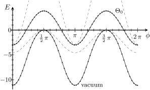
At large $L$, numerical results can be compared to large-L expressions of the energy (Lรผscher corrections). These large L expressions are obtained from (27) where the T-functions are replaced with their large-$L$ expression, which can be obtained for instance by setting $T_{1,-1}^{R}=0$ in (25). On figures Fig.1 and Fig.2 these large L energies are plotted in gray, while numeric energies of the vacuum and the state $\Theta_{0}$ are plotted in black. We see that the energy of the states are smooth functions of the twist, which converge, in the $\phi\to 0$ limit, to the periodic modelโ€™s vacuum energy and mass gap, which were already produced in the literature Balog:2003yr .

Refer to caption
Figure 1: Energies of vacuum and $\Theta_{0}$ as functions of twist at $L=1$. Dashed gray lines are the large $L$ expression of energy as a function of twist. In all numerical calculations we put $m=1$.
Refer to caption
Figure 2: Energies of vacuum and $\Theta_{0}$ as functions of twist at $L=1/10$. Deviation from the dashed gray lines shows the importance of finite-size effects.
Refer to caption
Figure 3: Energy of the state $\Theta_{0}$ at twist $\phi=\pi/2$. Crosses are numeric results and the dashed gray line is a linear fit. In spite of the limited numeric precision, it is manifest that at small $L$, $\frac{1}{E\,L}$ scales linearly with $\log L$.

VII Discussion

One of the main results of this paper is the observation that the vacuum energy is exactly zero at the special twist $\Omega$. Such behaviour is highly surprising in the absence of supersymmetry which could produce a vanishing vacuum energy by the mechanism of cancellation between fermionic and bosonic degrees of freedom333The gauge theory with $N=\infty$ compactified on the small 3d sphere Basar:2014hda provides another interesting example of theory with zero vacuum energy but without susy.. In the language of integrability this vacuum state looks very similar to the vacuum state in deformed AdS/CFT Ahn:2011xq ; Kazakov:2015efa ; Arutyunov:2010gu which has exactly zero energy at the trivial twist, but in $\mathcal{N}=4$ SYM it is just a consequence of unbroken supersymmetry. It would certainly be fascinating to understand the underlying mechanism or symmetry which is responsible for vanishing of vacuum energy in our case.

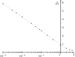
In the case of vacuum state the vanishing middle-node Y-functions $Y_{a,0}$ can be interpreted as the vanishing of densities $\rho^{a,0}$ of massive particles what makes it similar to the vacuum at $L=\infty$. It is most likely related to the idea of adiabatic continuity proposed in Cherman:2013yfa . Using resurgence techniques the authors of Cherman:2013yfa also proposed that the mass gap has confined form and scales as $\sim L$ at small $L$. As we see from Fig.3 the state $\Theta_{0}$ scales as in the weak coupling regime and is proportional to $\frac{1}{L\log L}$. One can expect that in the presence of the twist, the mass gap is not the difference of energies of the state $\Theta_{0}$ and vacuum. Probably another state has lower energy than the state $\Theta_{0}$, and that either this state does not correspond to a physical solution of Y-system in the periodic case, or that it is the same solution as vacuum in this limit. This would be similar to what happens for $SU(2)$ Heisenberg spin chains where the introduction of a twist lifts the degeneracy of some states belonging to the same multiplet, including states in the multiplet of vacuum. At the level of the Y-system (or equivalent finite system of integral equations), the search of the corresponding state is not a trivial task and should be addressed in a future paper.

Acknowledgements.

Acknowledgments

We thank D. Dorigoni, V. Kazakov, V. Schomerus and D. Volin for many fruitful and interesting discussions. The work of E.S. was supported by the People Programme (Marie Curie Actions) of the European Unionโ€™s Seventh Framework Programme FP7/2007-2013/ under REA Grant Agreement No 317089 (GATIS). S.L. thanks the centre de calcul de lโ€™universitรฉ de Bourgogne for providing computation ressources.

References

  • (1) P.ย B.ย Wiegmann, Phys.ย Lett.ย B 141 (1984) 217. doi:10.1016/0370-2693(84)90205-3
  • (2) E.ย Ogievetsky, P.ย Wiegmann and N.ย Reshetikhin, Nucl.ย Phys.ย B 280 (1987) 45. doi:10.1016/0550-3213(87)90138-6
  • (3) V.ย Kazakov and S.ย Leurent, arXiv:1007.1770 [hep-th]. doi:10.1016/j.nuclphysb.2015.11.012
  • (4) A.ย Cherman, D.ย Dorigoni, G.ย V.ย Dunne and M.ย รœnsal, Phys.ย Rev.ย Lett.ย  112 (2014) 021601 doi:10.1103/PhysRevLett.112.021601 [arXiv:1308.0127 [hep-th]].
  • (5) C.ย Ahn, Z.ย Bajnok, D.ย Bombardelli and R.ย I.ย Nepomechie, JHEP 1112 (2011) 059 doi:10.1007/JHEP12(2011)059 [arXiv:1108.4914 [hep-th]].
  • (6) A.ย Cherman, D.ย Dorigoni and M.ย Unsal, JHEP 1510 (2015) 056 doi:10.1007/JHEP10(2015)056 [arXiv:1403.1277 [hep-th]].
  • (7) N.ย Gromov, V.ย Kazakov and P.ย Vieira, JHEP 0912 (2009) 060 doi:10.1088/1126-6708/2009/12/060 [arXiv:0812.5091 [hep-th]].
  • (8) J.ย Balog and A.ย Hegedus, J.ย Phys.ย A 37 (2004) 1881 doi:10.1088/0305-4470/37/5/027 [hep-th/0309009].
  • (9) G.ย Basar, A.ย Cherman, D.ย A.ย McGady and M.ย Yamazaki, Phys.ย Rev.ย Lett.ย  114 (2015) 251604 doi:10.1103/PhysRevLett.114.251604 [arXiv:1408.3120 [hep-th]].
  • (10) V.ย Kazakov, S.ย Leurent and D.ย Volin, arXiv:1510.02100 [hep-th].
  • (11) G.ย Arutyunov, M.ย de Leeuw and S.ย J.ย van Tongeren, JHEP 1102 (2011) 025 doi:10.1007/JHEP02(2011)025 [arXiv:1009.4118 [hep-th]].