Distributed Machine Learning via Sufficient Factor Broadcasting

Distributed Machine Learning via Sufficient Factor Broadcasting

Abstract

Matrix-parametrized models, including multiclass logistic regression and sparse coding, are used in machine learning (ML) applications ranging from computer vision to computational biology. When these models are applied to large-scale ML problems starting at millions of samples and tens of thousands of classes, their parameter matrix can grow at an unexpected rate, resulting in high parameter synchronization costs that greatly slow down distributed learning. To address this issue, we propose a Sufficient Factor Broadcasting (SFB) computation model for efficient distributed learning of a large family of matrix-parameterized models, which share the following property: the parameter update computed on each data sample is a rank-1 matrix, i.e. the outer product of two “sufficient factors” (SFs). By broadcasting the SFs among worker machines and reconstructing the update matrices locally at each worker, SFB improves communication efficiency — communication costs are linear in the parameter matrix’s dimensions, rather than quadratic — without affecting computational correctness. We present a theoretical convergence analysis of SFB, and empirically corroborate its efficiency on four different matrix-parametrized ML models.

1 Introduction

For many popular machine learning (ML) models, such as multiclass logistic regression (MLR), neural networks (NN) [7], distance metric learning (DML) [35] and sparse coding [24], their parameters can be represented by a matrix $\mathbf{W}$. For example, in MLR, rows of $\mathbf{W}$ represent the classification coefficient vectors corresponding to different classes; whereas in SC rows of $\mathbf{W}$ correspond to the basis vectors used for reconstructing the observed data. A learning algorithm, such as stochastic gradient descent (SGD), would iteratively compute an update $\Delta\mathbf{W}$ from data, to be aggregated with the current version of $\mathbf{W}$. We call such models matrix-parameterized models (MPMs).

Learning MPMs in large scale ML problems is challenging: ML application scales have risen dramatically, a good example being the ImageNet [12] compendium with millions of images grouped into tens of thousands of classes. To ensure fast running times when scaling up MPMs to such large problems, it is desirable to turn to distributed computation; however, a unique challenge to MPMs is that the parameter matrix grows rapidly with problem size, causing straightforward parallelization strategies to perform less ideally. Consider a data-parallel algorithm, in which every worker uses a subset of the data to update the parameters — a common paradigm is to synchronize the full parameter matrix and update matrices amongst all workers [11, 10, 21, 7, 29, 14]. However, this synchronization can quickly become a bottleneck: take MLR for example, in which the parameter matrix $\mathbf{W}$ is of size $J\times D$, where $J$ is the number of classes and $D$ is the feature dimensionality. In one application of MLR to Wikipedia [26], $J=325$k and $D>10,000$, thus $\mathbf{W}$ contains several billion entries (tens of GBs of memory). Because typical computer cluster networks can only transfer a few GBs per second at the most, inter-machine synchronization of $\mathbf{W}$ can dominate and bottleneck the actual algorithmic computation. In recent years, many distributed frameworks have been developed for large scale machine learning, including Bulk Synchronous Parallel (BSP) systems such as Hadoop [11] and Spark [38], graph computation frameworks such as Pregel [23], GraphLab [13], and bounded-asynchronous key-value stores such as Yahoo LDA[2], DistBelief[10], Petuum-PS [15], Project Adam [7] and [22]. When using these systems to learn MPMs, it is common to transmit the full parameter matrices $\mathbf{W}$ and/or matrix updates $\Delta\mathbf{W}$ between machines, usually in a server-client style [11, 10, 29, 14, 7, 21]. As the matrices become larger due to increasing problem sizes, so do communication costs and synchronization delays — hence, reducing such costs is a key priority when using these frameworks.

In this paper, we investigate the structure of matrix parameterized models, in order to design efficient communication strategies that can be realized in distributed ML frameworks. We focus on models with a common property: when the parameter matrix $\mathbf{W}$ of these models is optimized with stochastic gradient descent (SGD) [10, 15, 7] or stochastic dual coordinate ascent (SDCA) [16, 27, 36, 18, 17], the update $\bigtriangleup\mathbf{W}$ computed over one (or a few) data sample(s) is of low-rank, e.g. it can be written as the outer product of two vectors $\mathbf{u}$ and $\mathbf{v}$: $\bigtriangleup\mathbf{W}=\mathbf{u}\mathbf{v}^{\top}$. The vectors $\mathbf{u}$ and $\mathbf{v}$ are sufficient factors (SF, meaning that they are sufficient to reconstruct the update matrix $\bigtriangleup\mathbf{W}$). A rich set of models [24, 19, 35, 37, 7] fall into this family: for instance, when solving an MLR problem using SGD, the stochastic gradient is $\bigtriangleup\mathbf{W}=\mathbf{u}\mathbf{v}^{\top}$, where $\mathbf{u}$ is the prediction probability vector and $\mathbf{v}$ is the feature vector. Similarly, when solving an $\ell_{2}$ regularized MLR problem using SDCA, the update matrix $\bigtriangleup\mathbf{W}$ also admits such as a structure, where $\mathbf{u}$ is the update vector of a dual variable and $\mathbf{v}$ is the feature vector. Other models include neural networks [7], distance metric learning [35], sparse coding [24], non-negative matrix factorization [19], principal component analysis, and group Lasso [37].

Leveraging this property, we propose a computation model called Sufficient Factor Broadcasting (SFB), and evaluate its effectiveness in a peer-to-peer implementation (while noting that SFB can also be used in other distributed frameworks). SFB efficiently learns parameter matrices using the SGD or SDCA algorithms, which are widely-used in distributed ML [16, 10, 15, 27, 36, 18, 7, 17, 21]. The basic idea is as follows: since $\bigtriangleup\mathbf{W}$ can be exactly constructed from the sufficient factors, rather than communicating the full (update) matrix between workers, we can instead broadcast only the sufficient factors and have workers reconstruct the updates. SFB is thus highly communication-efficient; transmission costs are linear in the dimensions of the parameter matrix, and the resulting faster communication greatly reduces waiting time in synchronous systems (e.g. Hadoop and Spark), or improves parameter freshness in (bounded) asynchronous systems (e.g. GraphLab, Petuum-PS and [22]). SFs have been used to speed up some (but not all) network communication in deep learning [7]; our work differs primarily in that we always transmit SFs, never full matrices.

SFB does not impose strong requirements on the distributed system — it can be used with synchronous [11, 23, 38], asynchronous [13, 2, 10], and bounded-asynchronous consistency models [5, 15, 31], in order to trade off between system efficiency and algorithmic accuracy. We provide theoretical analysis of SFB under synchronous and bounded-async consistency, and demonstrate that SFB learning of matrix-parametrized models significantly outperforms strategies that communicate the full parameter/update matrix, on a variety of applications including distance metric learning [35], sparse coding [24] and unregularized/$\ell_{2}$-regularized multiclass logistic regression. Using our own C++ implementations of each application, our experiments show that, for parameter matrices with 5-10 billion entries, replacing full-matrix communication with SFB improves convergence times by 3-4 fold. Notably, our SFB implementation of $\ell_{2}$-MLR is approximately 9 times faster than the Spark v1.3.1 implementation. We expect the performance benefit of SFB (versus full matrix communication) to improve with even larger matrix sizes.

The major contributions of this paper are summarized as follows:

• We identify the sufficient factor property of a large family of matrix-parametrized models when solved with two popular algorithms: stochastic gradient descent and stochastic dual coordinate ascent.

• In light of the sufficient factor property, we propose a sufficient factor broadcasting model of computation, which can greatly reduce the communication complexity without losing computational correctness.

• We provide an efficient implementation of SFB, with flexible consistency models and easy-to-use programming interface.

• We analyze the communication and computation costs of SFB and provide a convergence guarantee of SFB based minibatch SGD algorithm.

• We perform extensive evaluation of SFB on four popular models and corroborate the efficiency and low communication complexity of SFB.

The rest of the paper is organized as follows. In Section 2 and 3, we introduce the sufficient factor property of matrix-parametrized models and propose the sufficient factor broadcasting computation model, respectively. Section 4 presents SFBroadcaster, an implementation of SFB. Section 5 analyzes the costs and convergence behavior of SFB. Section 6 gives experimental results. Section 7 reviews related works and Section 8 concludes the paper.

2 Sufficient Factor Property of Matrix-Parametrized Models

The core goal of Sufficient Factor Broadcasting (SFB) is to reduce network communication costs for matrix-parametrized models; specifically, those that follow an optimization formulation

$$\textbf{(P)}\quad\begin{matrix}\underset{\mathbf{W}}{\textrm{min}}&\frac{1}{N}\sum\limits_{i=1}^{N}f_{i}(\mathbf{W}\mathbf{a}_{i})+h(\mathbf{W})\\ \end{matrix}$$ (1)

where the model is parametrized by a matrix $\mathbf{W}\in\mathds{R}^{J\times D}$. The loss function $f_{i}(\cdot)$ is typically defined over a set of training samples $\{(\mathbf{a}_{i},\mathbf{b}_{i})\}_{i=1}^{N}$, with the dependence on $\mathbf{b}_{i}$ being suppressed. We allow $f_{i}(\cdot)$ to be either convex or nonconvex, smooth or nonsmooth (with subgradient everywhere); examples include $\ell_{2}$ loss and multiclass logistic loss, amongst others. The regularizer $h(\mathbf{W})$ is assumed to admit an efficient proximal operator $\textrm{prox}_{h}(\cdot)$ [3]. For example, $h(\cdot)$ could be an indicator function of convex constraints, $\ell_{1}$-, $\ell_{2}$-, trace-norm, to name a few. The vectors $\mathbf{a}_{i}$ and $\mathbf{b}_{i}$ can represent observed features, supervised information (e.g., class labels in classification, response values in regression), or even unobserved auxiliary information (such as sparse codes in sparse coding [24]) associated with data sample $i$. The key property we exploit below ranges from the matrix-vector multiplication $\mathbf{W}\mathbf{a}_{i}$. This optimization problem (P) can be used to represent a rich set of ML models [24, 19, 35, 37, 7], such as the following:

Distance metric learning (DML) [35] improves the performance of other ML algorithms, by learning a new distance function that correctly represents similar and dissimilar pairs of data samples; this distance function is a matrix $\mathbf{W}$ that can have billions of parameters or more, depending on the data sample dimensionality. The vector $\mathbf{a}_{i}$ is the difference of the feature vectors in the $i$th data pair and $f_{i}(\cdot)$ can be either a quadratic function or a hinge loss function, depending on the similarity/dissimilarity label $\mathbf{b}_{i}$ of the data pair. In both cases, $h(\cdot)$ can be an $\ell_{1}$-, $\ell_{2}$-, trace-norm regularizer or simply $h(\cdot)=0$ (no regularization).

Sparse coding (SC) [24] learns a dictionary of basis from data, so that the data can be re-represented sparsely (and thus efficiently) in terms of the dictionary. In SC, $\mathbf{W}$ is the dictionary matrix, $\mathbf{a}_{i}$ are the sparse codes, $\mathbf{b}_{i}$ is the input feature vector and $f_{i}(\cdot)$ is a quadratic function [24]. To prevent the entries in $\mathbf{W}$ from becoming too large, each column $\mathbf{W}_{k}$ must satisfy $\|\mathbf{W}_{k}\|_{2}\leq 1$. In this case, $h(\mathbf{W})$ is an indicator function which equals 0 if $\mathbf{W}$ satisfies the constraints and equals $\infty$ otherwise.

2.1 Optimization via proximal SGD and SDCA

To solve the optimization problem (P), it is common to employ either (proximal) stochastic gradient descent (SGD) [10, 15, 7, 21] or stochastic dual coordinate ascent (SDCA) [16, 27, 36, 18, 17], both of which are popular and well-established parallel optimization techniques.

Proximal SGD: In proximal SGD, a stochastic estimate of the gradient, $\bigtriangleup\mathbf{W}$, is first computed over one data sample (or a mini-batch of samples), in order to update $\mathbf{W}$ via $\mathbf{W}\leftarrow\mathbf{W}-\eta\bigtriangleup\mathbf{W}$ (where $\eta$ is the learning rate). Following this, the proximal operator $\textrm{prox}_{\eta h}(\cdot)$ is applied to $\mathbf{W}$. Notably, the stochastic gradient $\bigtriangleup\mathbf{W}$ in (P) can be written as the outer product of two vectors $\bigtriangleup\mathbf{W}=\mathbf{u}\mathbf{v}^{\top}$, where $\mathbf{u}=\frac{\partial f(\mathbf{W}\mathbf{a}_{i},\mathbf{b}_{i})}{\partial(\mathbf{W}\mathbf{a}_{i})}$, $\mathbf{v}=\mathbf{a}_{i}$, according to the chain rule. Later, we will show that this low rank structure of $\bigtriangleup\mathbf{W}$ can greatly reduce inter-worker communication.

Stochastic DCA: SDCA applies to problems (P) where $f_{i}(\cdot)$ is convex and $h(\cdot)$ is strongly convex [36] (e.g. when $h(\cdot)$ contains the squared $\ell_{2}$ norm); it solves the dual problem of (P), via stochastic coordinate ascent on the dual variables. More specifically, introducing the dual matrix $\mathbf{U}=[\mathbf{u}_{1},\ldots,\mathbf{u}_{N}]\in\mathds{R}^{J\times N}$ and the data matrix $\mathbf{A}=[\mathbf{a}_{1},\ldots,\mathbf{a}_{N}]\in\mathds{R}^{D\times N}$, we can write the dual problem of (P) as

$$\textbf{(D)}\quad\begin{matrix}\underset{\mathbf{U}}{\textrm{min}}&\frac{1}{N}\sum\limits_{i=1}^{N}f_{i}^{*}(-\mathbf{u}_{i})+h^{*}(\frac{1}{N}\mathbf{U}\mathbf{A}^{\top})\end{matrix}$$ (2)

where $f_{i}^{*}(\cdot)$ and $h^{*}(\cdot)$ are the Fenchel conjugate functions of $f_{i}(\cdot)$ and $h(\cdot)$, respectively. The primal-dual matrices $\mathbf{W}$ and $\mathbf{U}$ are connected by $\mathbf{W}=\nabla h^{*}(\mathbf{Z})$, where the auxiliary matrix $\mathbf{Z}:=\tfrac{1}{N}\mathbf{U}\mathbf{A}^{\top}$. Algorithmically, we need to update the dual matrix $\mathbf{U}$, the primal matrix $\mathbf{W}$, and the auxiliary matrix $\mathbf{Z}$: every iteration, we pick a random data sample $i$, and compute the stochastic update $\bigtriangleup\mathbf{u}_{i}$ by minimizing (D) while holding $\{\mathbf{u}_{j}\}_{j\neq i}$ fixed. The dual variable is updated via $\mathbf{u}_{i}\leftarrow\mathbf{u}_{i}-\bigtriangleup\mathbf{u}_{i}$, the auxiliary variable via $\mathbf{Z}\leftarrow\mathbf{Z}-\bigtriangleup\mathbf{u}_{i}\mathbf{a}^{\top}_{i}$, and the primal variable via $\mathbf{W}\leftarrow\nabla h^{*}(\mathbf{Z})$. Similar to SGD, the update of the SDCA auxiliary variable $\mathbf{Z}$ is also the outer product of two vectors: $\bigtriangleup\mathbf{u}_{i}$ and $\mathbf{a}_{i}$, which can be exploited to reduce communication cost.

Sufficient Factor property in SGD and SDCA: In both SGD and SDCA, the parameter matrix update can be computed as the outer product of two vectors — we call these sufficient factors (SFs). This property can be leveraged to improve the communication efficiency of distributed ML systems: instead of communicating parameter/update matrices among machines, we can communicate the SFs and reconstruct the update matrices locally at each machine. Because the SFs are much smaller in size, synchronization costs can be dramatically reduced. See Section 5 below for a detailed analysis.

Low-rank Extensions: More generally, the update matrix $\bigtriangleup\mathbf{W}$ may not be exactly rank-1, but still of very low rank. For example, when each machine uses a mini-batch of size $K$, $\bigtriangleup\mathbf{W}$ is of rank at most $K$; in Restricted Boltzmann Machines [30], the update of the weight matrix is computed from four vectors $\mathbf{u}_{1},\mathbf{v}_{1},\mathbf{u}_{2},\mathbf{v}_{2}$ as $\mathbf{u}_{1}\mathbf{v}_{1}^{\top}-\mathbf{u}_{2}\mathbf{v}_{2}^{\top}$, i.e. rank-2; for the BFGS algorithm [4], the update of the inverse Hessian is computed from two vectors $\mathbf{u},\mathbf{v}$ as $\alpha\mathbf{u}\mathbf{u}^{\top}-\beta(\mathbf{u}\mathbf{v}^{\top}+\mathbf{v}\mathbf{u}^{\top})$, i.e. rank-3. Even when the update matrix $\bigtriangleup\mathbf{W}$ is not genuinely low-rank, to reduce communication cost, it might still make sense to send only a certain low-rank approximation. We intend to investigate these possibilities in future work.

3 Sufficient Factor Broadcasting

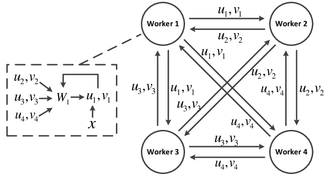
Figure 1: Sufficient Factor Broadcasting (SFB).

Leveraging the SF property of the update matrix in problems (P) and (D), we propose a Sufficient Factor Broadcasting (SFB) model of computation, that supports efficient (low-communication) distributed learning of the parameter matrix $\mathbf{W}$. We assume a setting with $P$ workers, each of which holds a data shard and a copy of the parameter matrix $\mathbf{W}$. Stochastic updates to $\mathbf{W}$ are generated via proximal SGD or SDCA, and communicated between machines to ensure parameter consistency. In proximal SGD, on every iteration, each worker $p$ computes SFs $(\mathbf{u}_{p},\mathbf{v}_{p})$, based on one data sample $\mathbf{x}_{i}=(\mathbf{a}_{i},\mathbf{b}_{i})$ in the worker’s data shard. The worker then broadcasts $(\mathbf{u}_{p},\mathbf{v}_{p})$ to all other workers; once all $P$ workers have performed their broadcast (and have thus received all SFs), they re-construct the $P$ update matrices (one per data sample) from the $P$ SFs, and apply them to update their local copy of $\mathbf{W}$. Finally, each worker applies the proximal operator $\textrm{prox}_{h}(\cdot)$. When using SDCA, the above procedure is instead used to broadcast SFs for the auxiliary matrix $\mathbf{Z}$, which is then used to obtain the primal matrix $\mathbf{W}=\nabla h^{*}(\mathbf{Z})$. Figure 1 illustrates SFB operation: 4 workers compute their respective SFs $(\mathbf{u}_{1},\mathbf{v}_{1})$, $\dots$, $(\mathbf{u}_{4},\mathbf{v}_{4})$, which are then broadcast to the other 3 workers. Each worker $p$ uses all 4 SFs $(\mathbf{u}_{1},\mathbf{v}_{1}),\dots,(\mathbf{u}_{4},\mathbf{v}_{4})$ to exactly reconstruct the update matrices $\bigtriangleup\mathbf{W}_{p}=\mathbf{u}_{p}\mathbf{v}_{p}^{\top}$, and update their local copy of the parameter matrix: $\mathbf{W}_{p}\leftarrow\mathbf{W}_{p}-\sum_{q=1}^{4}\mathbf{u}_{q}\mathbf{v}_{q}^{\top}$. While the above description reflects synchronous execution, asynchronous and bounded-asynchronous extensions are also possible (Section 4).

SFB vs client-server architectures: The SFB peer-to-peer topology can be contrasted with a “full-matrix” client-server architecture for parameter synchronization, e.g. as used by Project Adam [7] to learn neural networks: there, a centralized server maintains the global parameter matrix, and each client keeps a local copy. Clients compute sufficient factors and send them to the server, which uses the SFs to update the global parameter matrix; the server then sends the full, updated parameter matrix back to clients. Although client-to-server costs are reduced (by sending SFs), server-to-client costs are still expensive because full parameter matrices need to be sent. In contrast, the peer-to-peer SFB topology never sends full matrices; only SFs are sent over the network. We also note that under SFB, the update matrices are reconstructed at each of the $P$ machines, rather than once at a central server (for full-matrix architectures). Our experiments show that the time taken for update reconstruction is empirically negligible compared to communication and SF computation.

Mini-batch proximal SGD/SDCA: SFB can also be used in mini-batch proximal SGD/SDCA; every iteration, each worker samples a mini-batch of $K$ data points, and computes $K$ pairs of sufficient factors $\{(\mathbf{u}_{i},\mathbf{v}_{i})\}_{i=1}^{K}$. These $K$ pairs are broadcast to all other workers, which reconstruct the originating worker’s update matrix as $\bigtriangleup\mathbf{W}=\frac{1}{K}\sum_{i=1}^{K}\mathbf{u}_{i}\mathbf{v}_{i}^{\mathsf{T}}$.

4 Sufficient Factor Broadcaster: An Implementation

In this section, we present Sufficient Factor Broadcaster (SFBcaster) — an implementation of SFB — including consistency models, programing interface and implementation details. We stress that SFB does not require a special system; it can be implemented on top of existing distributed frameworks, using any suitable communication topology — such as star, ring, tree, fully-connected and Halton-sequence [21].

4.1 Flexible Consistency Models

Our SFBcaster implementation supports three consistency models: Bulk Synchronous Parallel (BSP-SFB), Asynchronous Parallel (ASP-SFB), and Stale Synchronous Parallel (SSP-SFB), and we provide theoretical convergence guarantees for BSP-SFB and SSP-SFB in the next section.

BSP-SFB: Under BSP [11, 23, 38], an end-of-iteration global barrier ensures all workers have completed their work, and synchronized their parameter copies, before proceeding to the next iteration. BSP is a strong consistency model, that guarantees the same computational outcome (and thus algorithm convergence) each time.

ASP-SFB: BSP can be sensitive to stragglers (slow workers) [15, 31], limiting the distributed system to the speed of the slowest worker.

The Asynchronous Parallel (ASP) [13, 2, 10] communication model addresses this issue, by allowing workers to proceed without waiting for others. ASP is efficient in terms of iteration throughput, but carries the risk that worker parameter copies can end up greatly out of synchronization, which can lead to algorithm divergence [15].

SSP-SFB: Stale Synchronous Parallel (SSP) [5, 15, 31] is a bounded-asynchronous consistency model that serves as a middle ground between BSP and ASP; it allows workers to advance at different rates, provided that the difference in iteration number between the slowest and fastest workers is no more than a user-provided staleness $s$. SSP alleviates the straggler issue while guaranteeing algorithm convergence [15, 31]. Under SSP-SFB, each worker $p$ tracks the number of SF pairs computed by itself, $t_{p}$, versus the number $\tau_{p}^{q}(t_{p})$ of SF pairs received from each worker $q$. If there exists a worker $q$ such that $t_{p}-\tau_{p}^{q}(t_{p})>s$ (i.e. some worker $q$ is likely more than $s$ iterations behind worker $p$), then worker $p$ pauses until $q$ is no longer $s$ iterations or more behind. When $s=0$, SSP-SFB reduces to BSP-SFB [11, 38], and when $s=\infty$, SSP-SFB becomes ASP-SFB.

4.2 Programming Interface

sfb_app mlr ( int J, int D, int staleness )

//SF computation function
function compute_sv ( sfb_app mlr ):

while ( ! converged ):

$X$ = sample_minibatch ()

foreach $\mathbf{x}_{i}$ in $X$:

//sufficient factor $\mathbf{u}_{i}$
       pred = predict ( mlr.para_mat, $\mathbf{x}_{i}$ )

mlr.sv_list[i].write_u ( pred )

//sufficient factor $\mathbf{v}_{i}$
       mlr.sv_list[i].write_v ( $\mathbf{x}_{i}$ )

commit()

Figure 2: Multiclass LR pseudocode.

sfb_app sc ( int D, int J , int staleness)

//SF computation function
function compute_sf ( sfb_app sc ):

while ( ! converge ):

$X$=sample_minibatch ()

foreach $\mathbf{x}_{i}$ in $X$:

//compute sparse code
       a = compute_sparse_code ( sc.para_mat, $\mathbf{x}_{i}$ )

//sufficient factor $\mathbf{u}_{i}$
       sc.sf_list[i].write_u ( sc.para_mat * a-$\mathbf{x}_{i}$ )

//sufficient factor $\mathbf{v}_{i}$
       sc.sf_list[i].write_v ( a )

commit()

//Proximal operator function
function prox ( sfb_app sc ):

foreach column $\mathbf{b}_{i}$ in sc.para_mat:

if $\|\mathbf{b}_{i}\|_{2}>1$:

$\mathbf{b}_{i}=\frac{\mathbf{b}_{i}}{\|\mathbf{b}_{i}\|_{2}}$

Figure 3: Sample code of sparse coding in SFB

The SFBcaster programming interface is simple; users need to provide a SF computation function to specify how to compute the sufficient factors. To send out SF pairs $(\mathbf{u},\mathbf{v})$, the user adds them to a buffer object $sv\_list$, via: $write\_u(vec\_u)$, $write\_v(vec\_v)$, which set $i$-th SF $\mathbf{u}$ or $\mathbf{v}$ to $vec\_u$ or $vec\_v$. All SF pairs are sent out at the end of an iteration, which is signaled by $commit()$. Finally, in order to choose between BSP, ASP and SSP consistency, users simply set $staleness$ to an appropriate value (0 for BSP, $\infty$ for ASP, all other values for SSP). SFBcaster automatically updates each worker’s local parameter matrix using all SF pairs — including both locally computed SF pairs added to $sv\_list$, as well as SF pairs received from other workers.

Figure 2 shows SFBcaster pseudocode for multiclass logistic regression. For proximal SGD/SDCA algorithms, SFBcaster requires users to write an additional function, $prox(mat)$, which applies the proximal operator $\textrm{prox}_{h}(\cdot)$ (or the SDCA dual operator $h^{*}(\cdot)$) to the parameter matrix $mat$. Figure 3 shows the sample code of implementing sparse coding in SFB. $D$ is the feature dimensionality of data and $J$ is the dictionary size. Users write a SF computation function to specify how to compute the sufficient factors: for each data sample $\mathbf{x}_{i}$, we first compute its sparse code $\mathbf{a}$ based on the dictionary $\mathbf{B}$ stored in the parameter matrix $sc.para\_mat$. Given $\mathbf{a}$, the sufficient factor $\mathbf{u}$ can be computed as $\mathbf{B}\mathbf{a}-\mathbf{x}_{i}$ and the sufficient factor $\mathbf{v}$ is simply $\mathbf{a}$. In addition, users provide a proximal operator function to specify how to project $\mathbf{B}$ to the $\ell_{2}$ ball constraint set.

4.3 Halton Sequence Broadcast

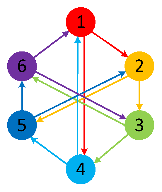
Figure 4: An Example of the Halton Sequence Broadcasting.

In previous sections, we assume the sufficient factors generated by each worker are broadcasted to all other workers. Such a full broadcast pattern incurs a communication cost $O(P^{2})$, which grows quadratically with the number of workers $P$. In data center scale clusters, $P$ can reach several thousand [10, 22], inwhere a full broadcast scheme would be too costly. To address this issue, we borrow the Halton-sequence idea proposed in [21], where each machine connects with and broadcasts messages to a subset of $Q$ machines rather than all other machines. $Q$ is in the scale of $\log P$, thereby, the communication cost can be greatly reduced. The basic idea of Halton sequence broadcast (HSB) [21] works as follows: given a constructed Halton sequence $\{P/2,P/4,3P/4,P/8,3P/8,\cdots\}$, each worker $p$ sends the sufficient vectors to $Q$ machines with IDs $\{$$(p+\lfloor P/2\rfloor)\%P$, $(p+\lfloor P/4\rfloor)\%P$, $(p+\lfloor 3P/4\rfloor)\%P$, $(p+\lfloor P/8\rfloor)\%P$, $(p+\lfloor 3P/8\rfloor)\%P$, $\cdots\}$. Figure 4 gives an illustration. In this example, we have 6 machines and set $Q=2\approx\log_{2}(6)$. According to the connection pattern rule, machine $p$ should broadcast messages to machine $(p+3)\%6$ and $(p+1)\%6$. For example, machine 1 broadcasts messages to machine 2 and 4; machine 5 broadcasts messages to machine 2 and 6. HSB loses per-iteration consistency of different parameter copies since each worker only broadcasts the sufficient vectors to part of peers. However, it pursues eventual consistency in the sense that over a period of time all the workers can see the effects of updates from every other worker directly or indirectly via an intermediate worker.

4.4 Implementation Details

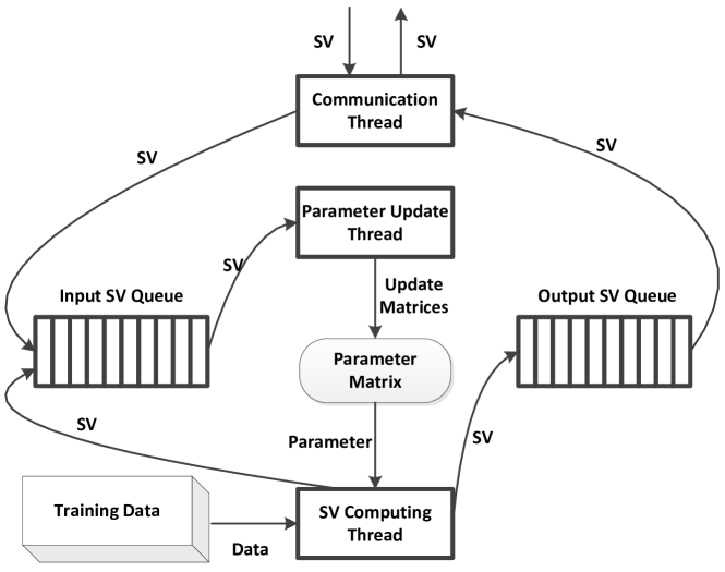
Figure 5: Implementation details on each worker in SFBcaster.

Figure 5 shows the implementation details on each worker in SFBcaster. Each worker maintains three threads: SF computing thread, parameter update thread and communication thread. Each worker holds a local copy of the parameter matrix and a partition of the training data. It also maintains an input SF queue which stores the sufficient factors computed locally and received remotely and an output SF queue which stores SFs to be sent to other workers. In each iteration, the SF computing thread checks the consistency policy detailed in Section 4 in the main paper. If permitted, this thread randomly chooses a minibatch of samples from the training data, computes the SFs and pushes them to the input and output SF queue. The parameter update thread fetches SFs from the input SF queue and uses them to update the parameter matrix. In proximal-SGD/SDCA, the proximal/dual operator function (provided by the user) is automatically called by this thread as a function pointer. The communication thread receives SFs from other workers and pushes them into the input SF queue and sends SFs in the output SF queue to other workers, either in a full broadcasting scheme or a Halton sequence based partial broadcasting scheme. One worker is in charge of measuring the objective value. Once the algorithm converges, this worker notifies all other workers to terminate the job. We implemented SFBcaster in C++. OpenMPI was used for communication between workers and OpenMP was used for multicore parallelization within each machine.

The decentralized architecture of SFBcaster makes it robust to machine failures. If one worker fails, the rest of workers can continue to compute and broadcast the sufficient factors among themselves. In addition, SFBcaster possesses high elasticity [22]: new workers can be added and existing workers can be taken offline, without restarting the running framework. A thorough study of fault tolerance and elasticity will be left for future work.

5 Cost Analysis and Theory

Computational Model	Total comms, per iter	$\mathbf{W}$ storage per machine	$\mathbf{W}$ update time, per iter
SFB (peer-to-peer, full broadcasting)	$O(P^{2}K(J+D))$	$O(JD)$	$O(P^{2}KJD)$
SFB (peer-to-peer, Halton sequence broadcasting)	$O(P\log PK(J+D))$	$O(JD)$	$O(P\log PKJD)$
FMS (client-server [7])	$O(PJD)$	$O(JD)$	$O(PJD)$ at server, $O(PKJD)$ at clients

Figure 6: Cost of using SFB versus FMS, where $K$ is minibatch size, $J,D$ are dimensions of $\mathbf{W}$, and $P$ is the number of workers.

We now examine the costs and convergence behavior of SFB under synchronous and bounded-async (e.g. SSP [5, 15, 8]) consistency, and show that SFB can be preferable to full-matrix synchronization/communication schemes.

5.1 Cost Analysis

Table 6 compares the communications, space and time (to apply updates to $\mathbf{W}$) costs of peer-to-peer SFB, against full matrix synchronization (FMS) under a client-server architecture [7]. For SFB with a full broadcasting scheme, in each minibatch, every worker broadcasts $K$ SF pairs $(\mathbf{u},\mathbf{v})$ to $P-1$ other workers, i.e. $O(P^{2}K(J+D))$ values are sent per iteration — linear in matrix dimensions $J,D$, and quadratic in $P$. For SFB with a Halton sequence broadcasting scheme, every worker communicates SF pairs with $Q=O(P)$ peers, hence the communication cost is reduced to $O(P\log PK(J+D))$. Because SF pairs cannot be aggregated before transmission, the cost has a dependency on $K$. In contrast, the communication cost in FMS is $O(PJD)$, linear in $P$, quadratic in matrix dimensions, and independent of $K$. For both SFB and FMS, the cost of storing $\mathbf{W}$ is $O(JD)$ on every machine. As for the time taken to update $\mathbf{W}$ per iteration, FMS costs $O(PJD)$ at the server (to aggregate $P$ client update matrices) and $O(PKJD)$ at the $P$ clients (to aggregate $K$ updates into one update matrix for the server). By comparison, SFB bears a cost of $O(P^{2}KJD)$ under full broadcasting and $O(P\log PKJD)$ under Halton sequence broadcasting due to the additional overhead of reconstructing each update matrix $P$ times.

Compared with FMS, SFB achieves communication savings by paying an extra computation cost. In a number of practical scenarios, such a tradeoff is worthwhile. Consider large problem scales where $\min(J,D)\geq 10000$, and moderate minibatch sizes $1\leq K\leq 1000$ (as studied in this paper); when using a moderate number of machines (around 10-100), the $O(P^{2}K(J+D))$ communications cost of SFB is lower than the $O(PJD)$ cost for FMS, and the relative benefit of SFB improves as the dimensions $J,D$ of $\mathbf{W}$ grow. In data center scale computing environments with thousands of machines, we can adopt the Halton sequence broadcasting scheme under which the communication cost is linearithmic ($O(P\log P)$) in $P$. As for the time needed to apply updates to $\mathbf{W}$, it turns out that the additional cost of reconstructing each update matrix $P$ times in SFB is negligible in practice — we have observed in our experiments that the time spent computing SFs, as well as communicating SFs over the network, greatly dominates the cost of reconstructing update matrices using SFs. Overall, the communication savings dominate the added computational overhead, which we validated in experiments (Section 6).

5.2 Convergence Analysis

We study the convergence of minibatch SGD under full broadcasting SFB (with extensions to proximal-SGD, SDCA and Halton sequence broadcasting being a topic for future study). Since SFB is a peer-to-peer decentralized computation model, we need to show the parameter copies on different workers converge to the same limiting point. This is different from the analyses of centralized parameter server systems [15, 8, 1], which show convergence of global parameters on the central server.

We wish to solve the optimization problem $\min_{\mathbf{W}}~{}\sum_{m=1}^{M}$ $f_{m}(\mathbf{W})$, where $M$ is the number of training data minibatches, and $f_{m}$ corresponds to the loss function on the $m$-th minibatch. Assume the training data minibatches $\{1,...,M\}$ are divided into $P$ disjoint subsets $\{S_{1},...,S_{P}\}$ with $|S_{p}|$ denoting the number of minibatches in $S_{p}$. Denote $F=\sum_{m=1}^{M}f_{m}$ as the total loss, and for $p=1,\ldots,P$, $F_{p}:=\sum_{j\in S_{p}}f_{j}$ is the loss on $S_{p}$ (residing on the $p$-th machine).

Consider a distributed system with $P$ machines. Each machine $p$ keeps a local variable $\mathbf{W}_{p}$ and the training data in $S_{p}$. At each iteration, machine $p$ draws one minibatch $I_{p}$ uniformly at random from partition $S_{p}$, and computes the partial gradient $\sum_{j\in I_{p}}\nabla f_{j}(\mathbf{W}_{p})$. Each machine updates its local variable by accumulating partial updates from all machines. Denote $\eta_{c}$ as the learning rate at $c$-th iteration on every machine. The partial update generated by machine $p$ at its $c$-th iteration is denoted as $U_{p}(\mathbf{W}_{p}^{c},I_{p}^{c})=-\eta_{c}|S_{p}|\sum_{j\in I_{p}^{c}}\nabla f_{j}(\mathbf{W}_{p}^{c})$. Note that $I_{p}^{c}$ is random and the factor $|S_{p}|$ is to restore unbiasedness in expectation. Then the local update rule of machine $p$ is

$$\textstyle\mathbf{W}_{p}^{c}=\mathbf{W^{0}}+\sum_{q=1}^{P}\sum_{t=0}^{\tau_{p}^{q}(c)}U_{q}(\mathbf{W}_{q}^{t},I_{q}^{t}),\quad 0\leq(c-1)-\tau_{p}^{q}(c)\leq s$$ (3)

where $\mathbf{W}^{0}$ is the common initializer for all $P$ machines, and $\tau_{p}^{q}(c)$ is the number of iterations machine $q$ has transmitted to machine $p$ when machine $p$ conducts its $c$-th iteration. Clearly, $\tau_{p}^{p}(c)=c$. Note that we also require $\tau_{p}^{q}(c)\leq c-1$, i.e., machine $p$ will not use any partial updates of machine $q$ that are too fast forward. This is to avoid correlation in the theoretical analysis. Hence, machine $p$ (at its $c$-th iteration) accumulates updates generated by machine $q$ up to iteration $\tau_{p}^{q}(c)$, which is restricted to be at most $s$ iterations behind. Such bounded-asynchronous communication addresses the slow-worker problem caused by bulk synchronous execution, while ensuring that the updates accumulated by each machine are not too outdated. The following standard assumptions are needed for our theoretical analysis:

Assumption 1

(1) For all $j$, $f_{j}$ is continuously differentiable and $F$ is bounded from below; (2) $\nabla F$, $\nabla F_{p}$ are Lipschitz continuous with constants $L_{F}$ and $L_{p}$, respectively, and let $L=\sum_{p=1}^{P}L_{p}$; (3) There exists $B,\sigma^{2}$ such that for all $p$ and $c$, we have (almost surely) $\|\mathbf{W}_{p}^{c}\|\leq B$ and $\mathbb{E}\|~{}|S_{p}|\sum_{j\in I_{p}}\nabla f_{j}(\mathbf{W})-\nabla F_{p}(\mathbf{W})~{}\|_{2}^{2}\leq\sigma^{2}$.

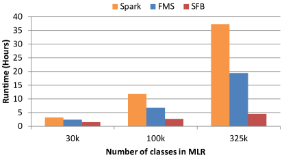
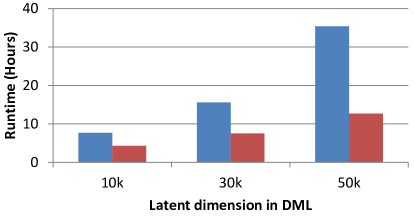
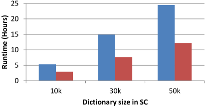
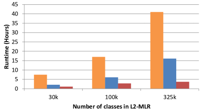
Figure 7: Convergence time versus model size for MLR, DML, SC, L2-MLR (left to right), under BSP.

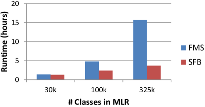
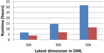
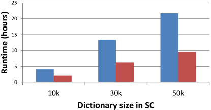
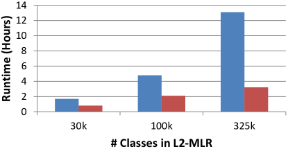
Figure 8: Convergence time versus model size for MLR, DML, SC, L2-MLR (left to right), under SSP with staleness=20.

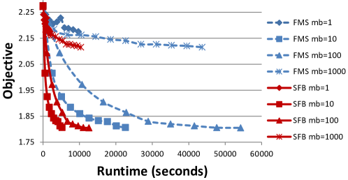
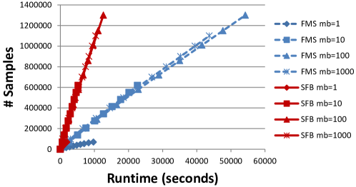
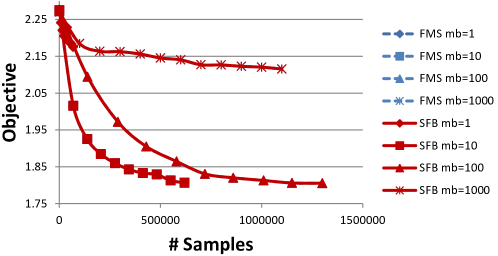
Figure 9: MLR objective vs runtime (left), samples vs runtime (middle), objective vs samples (right).

Our analysis is based on the following auxiliary update

$$\textstyle\mathbf{W}^{c} =\textstyle\mathbf{W}^{0}+\sum_{q=1}^{P}\sum_{t=0}^{c-1}U_{q}(\mathbf{W}_{q}^{t},I_{q}^{t}),$$ (4)

Compare to the local update (3) on machine $p$, essentially this auxiliary update accumulates all $c-1$ updates generated by all machines, instead of the $\tau_{p}^{q}(c)$ updates that machine $p$ has access to. We show that all local machine parameter sequences are asymptotically consistent with this auxiliary sequence:

Theorem 1

Let $\{\mathbf{W}_{p}^{c}\}$, $p=1,\ldots,P$, and $\{\mathbf{W}^{c}\}$ be the local sequences and the auxiliary sequence generated by SFB for problem (P) (with $h\equiv 0$), respectively. Under Assumption 1 and set the learning rate $\eta_{c}^{-1}=\frac{L_{F}}{2}+2sL+\sqrt{c}$, then we have

• $\liminf\limits_{c\to\infty}\mathbb{E}\|\nabla F(\mathbf{W}^{c})\|=0$, hence there exists a subsequence of $\nabla F(\mathbf{W}^{c})$ that almost surely vanishes;

• $\lim\limits_{c\to\infty}\max_{p}\|\mathbf{W}^{c}-\mathbf{W}_{p}^{c}\|=0$, i.e. the maximal disagreement between all local sequences and the auxiliary sequence converges to 0 (almost surely);

• There exists a common subsequence of $\{\mathbf{W}_{p}^{c}\}$ and $\{\mathbf{W}^{c}\}$ that converges almost surely to a stationary point of $F$, with the rate $\underset{c\leq C}{\mathrm{min}}~{}\mathbb{E}\|\sum_{p=1}^{P}\nabla F_{p}(\mathbf{W}_{p}^{c})\|_{2}^{2}\leq O\left(\frac{(L+L_{F})\sigma^{2}Ps\log C}{\sqrt{C}}\right)$

Intuitively, Theorem 1 says that, given a properly-chosen learning rate, all local worker parameters $\{\mathbf{W}^{c}_{p}\}$ eventually converge to stationary points (i.e. local minima) of the objective function $F$, despite the fact that SF transmission can be delayed by up to $s$ iterations. Thus, SFB learning is robust even under bounded-asynchronous communication (such as SSP). Our analysis differs from [5] in two ways: (1) [5] explicitly maintains a consensus model which would require transmitting the parameter matrix among worker machines — a communication bottleneck that we were able to avoid; (2) we allow subsampling in each worker machine. Accordingly, our theoretical guarantee is probabilistic, instead of the deterministic one in [5].

6 Experiments

We demonstrate how four popular models can be efficiently learnt using SFB: (1) multiclass logistic regression (MLR) and distance metric learning (DML) based on SGD; (2) sparse coding (SC) based on proximal SGD; (3) $\ell_{2}$ regularized multiclass logistic regression (L2-MLR) based on SDCA. For baselines, we compare with (a) Spark [38] for MLR and L2-MLR, and (b) full matrix synchronization (FMS) implemented on open-source parameter servers [15, 22] for all four models. In FMS, workers send update matrices to the central server, which then sends up-to-date parameter matrices to workers. Due to data sparsity, both the update matrices and sufficient factors are sparse; we use this fact to reduce communication and computation costs. Our experiments used a 12-machine cluster; each machine has 64 2.1GHz AMD cores, 128G memory, and a 10Gbps network interface.

6.1 Datasets and Experimental Setup

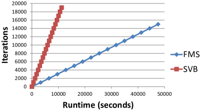
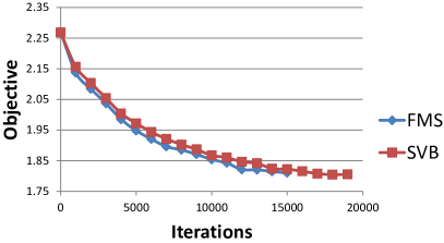
Figure 10: MLR iteration throughput (left) and iteration quality (right) under SSP (staleness=20).

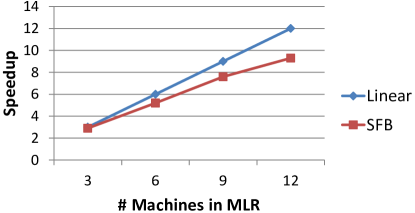
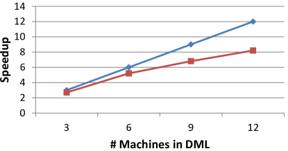
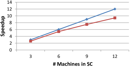
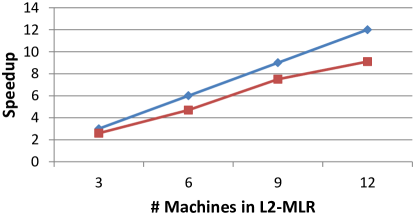
Figure 11: SFB scalability with varying machines under BSP, for MLR, DML, SC, L2-MLR (left to right).

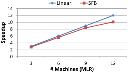
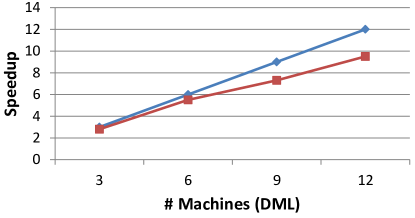
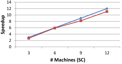
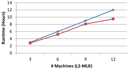
Figure 12: SFB scalability with varying machines, for MLR, DML, SC, L2-MLR (left to right), under SSP (staleness=20).

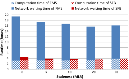
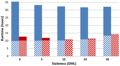
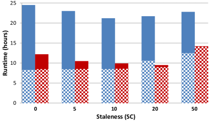
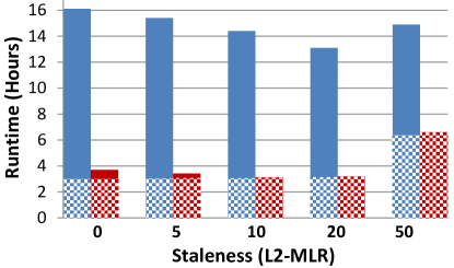
Figure 13: Computation vs network waiting time for MLR, DML, SC, L2-MLR (left to right).

We used two datasets for our experiments: (1) ImageNet [12] ILSFRC2012 dataset, which contains 1.2 million images from 1000 categories; the images are represented with LLC features [33], whose dimensionality is 172k. (2) Wikipedia [26] dataset, which contains 2.4 million documents from 325k categories; documents are represented with tf-idf, with a dimensionality of 20k. We ran MLR, DML, SC, L2-MLR on the Wikipedia, ImageNet, ImageNet, Wikipedia datasets respectively, and the parameter matrices contained up to 6.5b, 8.6b, 8.6b, 6.5b entries respectively (the largest latent dimension for DML and largest dictionary size for SC were both 50k). The tradeoff parameters in SC and L2-MLR were set to 0.001 and 0.1. We tuned the minibatch size, and found that $K=100$ was near-ideal for all experiments. All experiments used the same constant learning rate (tuned in the range $[10^{-5},1]$). In all experiments except those in Section 6.6, we adopted a full broadcasting scheme.

6.2 Convergence Speed and Quality

Figure 7 shows the time taken to reach a fixed objective value, for different model sizes, using BSP consistency. Figure 8 shows the results under SSP with staleness=20. SFB converges faster than FMS, as well as Spark v1.3.1. This is because SFB has lower communication costs, hence a greater proportion of running time gets spent on computation rather than network waiting. This is shown in Figure 9, which plots data samples processed per second (throughput) and algorithm progress per sample for MLR, under BSP consistency and varying minibatch sizes. The middle graph shows that SFB processes far more samples per second than FMS, while the rightmost graph shows that SFB and FMS produce exactly the same algorithm progress per sample under BSP. For this experiment, minibatch sizes between $K=10$ and 100 performed the best as indicated by the leftmost graph. We point out that larger model sizes should further improve SFB’s advantage over FMS, because SFB has linear communications cost in the matrix dimensions, whereas FMS has quadratic costs. Under a large model size (e.g., 325K classes in MLR), the communication cost becomes the bottleneck in FMS and causes prolonged network waiting time and considerable parameter synchronization delays, while the cost is moderate in SFB.

We also compared the iteration throughput and quality of SFB and FMS under the SSP consistency model. Figure 10 shows the iteration throughput (left) and iteration quality (right) for MLR, under SSP (staleness=20). The minibatch size was set to 100 for both SFB and FMS. As can be seen from the right graph, SFB has a slightly worse iteration quality than FMS. The reason we conjecture is the centralized architecture of FMS is more robust and stable than the decentralized architecture of SFB. On the other hand, the iteration throughput of SFB is much higher than FMS as shown in the left graph. Overall, SFB outperforms FMS in total convergence time.

6.3 Scalability

In all experiments that follow, we set the number of (L2)-MLR classes, DML latent dimension, SC dictionary size to 325k, 50k, 50k respectively. Figure 11 shows SFB scalability with varying machines under BSP, for MLR, DML, SC, L2-MLR. Figure 12 shows how SFB scales with machine count, under SSP with staleness=20. In general, we observed close to linear (ideal) speedup, with a slight drop at 12 machines.

6.4 Computation Time vs Network Waiting Time

Figure 13 shows the total computation and network time required for SFB and FMS to converge, across a range of SSP staleness values — in general, higher communication cost and lower staleness induce more network waiting. In the figure, the horizontal axis corresponds to different staleness values. The blue solid bar, blue checker board, red solid bar and red checker board correspond to the network waiting time of FMS, computation time of FMS, network waiting time of SFB and computation time of SFB respectively. For all staleness values, SFB requires far less network waiting (because SFs are much smaller than full matrices in FMS). Computation time for SFB is slightly longer than FMS because (1) update matrices must be reconstructed on each SFB worker, and (2) SFB requires a few more iterations for convergence, because peer-to-peer communication causes a slightly more parameter inconsistency under staleness. Overall, the SFB reduction in network waiting time remains far greater than the added computation time, and outperforms FMS in total time.

Another observation is that increasing staleness value can reduce the network waiting time for both FMS and SFB, thus allows more iterations to be performed in a given time interval. This is because a larger staleness gives each worker more flexibility to proceed at its own pace without waiting for others. On the other hand, as staleness increases, the computation time grows. If the staleness is too large (e.g., 50), the total convergence time is prolonged due to the rapid increasing of computation time. This is due to that the parameter copies on different workers bear a higher risk to be out of synchronization (thus inconsistent) under a larger staleness, which hurts the convergence quality of each iteration and requires more iterations to achieve the same objective value. The best tradeoff happens when staleness is around 10-20 in our experiments.

6.5 Communication Cost

Figure 14 shows the communication volume of four models under BSP. As shown in the figure, the communication volume of SFB is significantly lower than FMS and Spark. Under the BSP consistency model, SFB and FMS share the same iteration quality, hence need the same number of iterations to converge. Within each iteration, SFB communicates vectors while FMS transmits matrices. As a result, the communication volume of SFB is much lower than FMS.

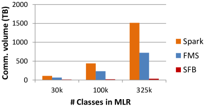
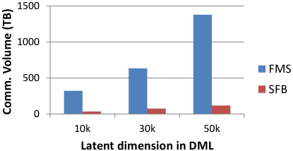
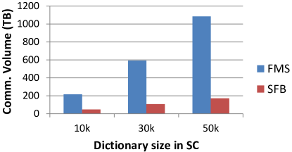
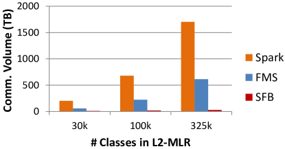
Figure 14: Communication volume for MLR, DML, SC, L2-MLR (left to right) under BSP.

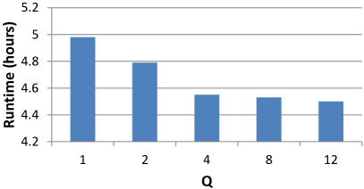
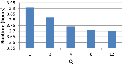
Figure 15: Convergence time versus Q in Halton sequence broadcasting for MLR (left) and L2-MLR (right), under BSP.

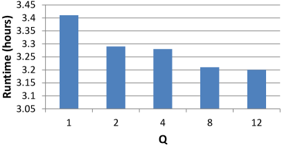
Figure 16: Convergence time versus Q in Halton sequence broadcasting for MLR (left) and L2-MLR (right), under SSP (staleness=20).

6.6 Halton Sequence Broadcasting

We studied how the parameter $Q$ in Halton sequence broadcasting (HSB) affects the convergence speed of SFB. Figure 15 and 16 show the convergence time of MLR and L2-MLR versus varying Q, under BSP and SSP (staleness=20) respectively. As observed in these two figures, a smaller $Q$ incurs longer convergence time. This is because a smaller $Q$ is more likely to cause the parameter copies on different workers to be out of synchronization and degrade iteration quality. However, as long as $Q$ is not too small, the convergence speed of HSB is comparable with a full broadcasting scheme. As shown in the figures, for $Q\geq 4\approx\log_{2}12$, the convergence time of HSB is very close to full broadcasting (where $Q=12$). This demonstrates that using HSB, we can reduce the communication cost from $O(P^{2})$ to $O(PQ)\approx O(P\log P)$ with slight sacrifice of the convergence speed.

7 Related Works

A number of system and algorithmic solutions have been proposed to reduce communication cost in distributed ML. On the system side, [10] proposed to reduce communication overhead by reducing the frequency of parameter/gradient exchanges between workers and the central server. [22] used filters to select part of “important” parameters/updates for transmission to reduce the number of data entries to be communicated. On the algorithm side, [32] and [36] studied the tradeoffs between communication and computation in distributed dual averaging and distributed stochastic dual coordinate ascent respectively. [28] proposed an approximate Newton-type method to achieve communication efficiency in distributed optimization. SFB is orthogonal to these existing approaches and be potentially combined with them to further reduce communication cost.

Peer-to-peer, decentralized architectures have been investigated in other distributed ML frameworks [6, 9, 25, 21]. Our SFBcaster system also adopt such an architecture, but with the specific purpose of supporting the SFB computation model, which is not explored by existing peer-to-peer ML frameworks.

8 Conclusions and Future Works

In this paper, we identify the sufficient factor property of a large set of matrix-parametrized models: when these models are optimized with stochastic gradient descent or stochastic dual coordinate ascent, the update matrices are of low-rank. Leveraging this property, we propose a sufficient factor broadcasting computation model to efficiently handle the learning of these models with low communication cost. We analyze the cost and convergence property of SFB and provide an efficient implementation and empirical evaluations.

For very large models, the size of the local parameter matrix $\mathbf{W}$ may exceed each machine’s memory capacity — to address this issue, we would like to investigate partitioning $\mathbf{W}$ over a small number of nearby machines, or using out-of-core (disk-based) storage to hold $\mathbf{W}$ in future work.

Finally, a promising extension to the SF idea is to re-parameterize the model $\mathbf{W}$ completely in terms of SFs, rather than just the updates. For example, if we initialize the parameter matrix $\mathbf{W}$ to be of low rank $R$, i.e., $\mathbf{W}^{0}=\sum_{j=1}^{R}\mathbf{u}_{j}\mathbf{v}_{j}^{\top}$, after $I$ iterations (updates), $\mathbf{W}^{I}=\sum_{j=1}^{R+I}\mathbf{u}_{j}\mathbf{v}_{j}^{\top}$. Leveraging this fact, for SGD without proximal operation and SDCA where $h(\cdot)$ is a $\ell_{2}$ regularizer, we can re-parametrize $\mathbf{W}^{I}$ using a set of SFs $\{(\mathbf{u}_{j},\mathbf{v}_{j})\}_{j=1}^{R+I}$, rather than maintaining $\mathbf{W}$ explicitly. This re-parametrization can possibly reduce both computation and storage cost, which we will investigate in the future.

Appendix A Proof of Theorem 1

Proof A.1.

Let $\mathcal{F}^{c}:=\sigma\{I_{p}^{\tau}:p=1,\ldots,P,\tau=1,\ldots,c\}$ be the filtration generated by the random samplings $I_{p}^{\tau}$ up to iteration counter $c$, i.e., the information up to iteration $c$. Note that for all $p$ and $c$, $\mathbf{W}_{p}^{c}$ and $\mathbf{W}^{c}$ are $\mathcal{F}^{c-1}$ measurable (since $\tau_{p}^{q}(c)\leq c-1$ by assumption), and $I_{p}^{c}$ is independent of $\mathcal{F}^{c-1}$. Recall that the partial update generated by machine $p$ at its $c$-th iteration is

$$U_{p}(\mathbf{W}_{p}^{c},I_{p}^{c})=-\eta_{c}|S_{p}|\sum_{j\in I_{p}^{c}}\nabla f_{j}(\mathbf{W}_{p}^{c})$$

Then it holds that

$$U_{p}(\mathbf{W}_{p}^{c})=\mathbb{E}[U_{p}(\mathbf{W}_{p}^{c},I_{p}^{c})|\mathcal{F}^{c-1}]=-\eta_{c}\nabla F_{p}(\mathbf{W}_{p}^{c})$$

(Note that we have suppressed the dependence of $U_{p}$ on the iteration counter $c$.)

Then, we have

$$\begin{array}[]{l}\mathbb{E}\left[\sum_{p=1}^{P}U_{p}(\mathbf{W}_{p}^{c},I_{p}^{c})~{}|~{}\mathcal{F}^{c-1}\right]=\sum_{p=1}^{P}\mathbb{E}[U_{p}(\mathbf{W}_{p}^{c},I_{p}^{c})~{}|~{}\mathcal{F}^{c-1}]\\ =\sum_{p=1}^{P}U_{p}(\mathbf{W}_{p}^{c})\end{array}$$ (5)

Similarly we have

$$\begin{array}[]{l}\mathbb{E}\left[\big{\|}\sum_{p=1}^{P}U_{p}(\mathbf{W}_{p}^{c},I_{p}^{c})\big{\|}_{2}^{2}~{}|~{}\mathcal{F}^{c-1}\right]\\ =\sum_{p,q=1}^{P}\mathbb{E}[\langle U_{p}(\mathbf{W}_{p}^{c},I_{p}^{c}),U_{q}(\mathbf{W}_{q}^{c},I_{q}^{c})\rangle~{}|~{}\mathcal{F}^{c-1}]\\ =\sum_{p,q=1}^{P}\langle U_{p}(\mathbf{W}_{q}^{c}),U_{q}(\mathbf{W}_{q}^{c})\rangle\\ +\sum_{p=1}^{P}\mathbb{E}\left[\|U_{p}(\mathbf{W}_{p}^{c},I_{p}^{c})-U_{p}(\mathbf{W}_{p}^{c})\|_{2}^{2}~{}|~{}\mathcal{F}^{c-1}\right]\end{array}$$ (6)

The variance term in the above equality can be bounded as

$$\begin{array}[]{l}\sum_{p=1}^{P}\mathbb{E}\left[\|U_{p}(\mathbf{W}_{p}^{c},I_{p}^{c})-U_{p}(\mathbf{W}_{p}^{c})\|_{2}^{2}~{}|~{}\mathcal{F}^{c-1}\right]\\ =\eta_{c}^{2}\underbrace{\sum_{p=1}^{P}\mathbb{E}\left[\||S_{p}|\sum_{j\in I_{p}^{c}}\nabla f_{j}(\mathbf{W}_{p}^{c})-\nabla F_{p}(\mathbf{W}_{p}^{c})\|_{2}^{2}~{}|~{}\mathcal{F}^{c-1}\right]}_{\hat{\sigma}^{2}P}\\ \leq\eta_{c}^{2}\hat{\sigma}^{2}P\end{array}$$ (7)

Now use the update rule $\mathbf{W}_{p}^{c+1}=\mathbf{W}_{p}^{c}+\sum_{p=1}^{P}U_{p}(\mathbf{W}_{p}^{c},I_{p}^{c})$ and the descent lemma [5], we have

$$\begin{array}[]{l}F(\mathbf{W}^{c+1})-F(\mathbf{W}^{c})\\ \leq\langle\mathbf{W}^{c+1}-\mathbf{W}^{c},\nabla F(\mathbf{W}^{c})\rangle+\frac{L_{F}}{2}\|\mathbf{W}^{c+1}-\mathbf{W}^{c}\|_{2}^{2}\\ =\langle\sum_{p=1}^{P}U_{p}(\mathbf{W}_{p}^{c},I_{p}^{c}),\nabla F(\mathbf{W}^{c})\rangle+\frac{L_{F}}{2}\|\sum_{p=1}^{P}U_{p}(\mathbf{W}_{p}^{c},I_{p}^{c})\|_{2}^{2}\end{array}$$ (8)

Then take expectation on both sides, we obtain

$$\begin{array}[]{l}\mathbb{E}\left[\right.\left.F(\mathbf{W}^{c+1})-F(\mathbf{W}^{c})~{}|~{}\mathcal{F}^{c-1}\right]\\ \leq\langle\sum_{p=1}^{P}U_{p}(\mathbf{W}_{p}^{c}),\nabla F(\mathbf{W}^{c})\rangle+\frac{L_{F}\eta_{c}^{2}\hat{\sigma}^{2}P}{2}\\ +\frac{L_{F}}{2}\|\sum_{p=1}^{P}U_{p}(\mathbf{W}_{p}^{c})\|_{2}^{2}\\ =(\frac{L_{F}}{2}-\eta_{c}^{-1})\|\sum_{p=1}^{P}U_{p}(\mathbf{W}_{p}^{c})\|_{2}^{2}+\frac{L_{F}\eta_{c}^{2}\hat{\sigma}^{2}P}{2}\\ -\eta_{c}^{-1}\langle\sum_{p=1}^{P}U_{p}(\mathbf{W}_{p}^{c}),\sum_{p=1}^{P}[U_{p}(\mathbf{W}^{c})-U_{p}(\mathbf{W}_{p}^{c})]\rangle\\ \leq(\frac{L_{F}}{2}-\eta_{c}^{-1})\|\sum_{p=1}^{P}U_{p}(\mathbf{W}_{p}^{c})\|_{2}^{2}+\frac{L_{F}\eta_{c}^{2}\hat{\sigma}^{2}P}{2}\\ +\|\sum_{p=1}^{P}U_{p}(\mathbf{W}_{p}^{c})\|\sum_{p=1}^{P}L_{p}\|\mathbf{W}^{c}-\mathbf{W}_{p}^{c}\|\end{array}$$ (9)

Now take expectation w.r.t all random variables, we obtain

$$\begin{array}[]{l}\mathbb{E}\left[F(\mathbf{W}^{c+1})-F(\mathbf{W}^{c})\right]\leq(\frac{L_{F}}{2}-\eta_{c}^{-1})\mathbb{E}\left[\|\sum_{p=1}^{P}U_{p}(\mathbf{W}_{p}^{c})\|_{2}^{2}\right]\\ +\sum_{p=1}^{P}L_{p}\mathbb{E}\left[\|\sum_{p=1}^{P}U_{p}(\mathbf{W}_{p}^{c})\|\|\mathbf{W}^{c}-\mathbf{W}_{p}^{c}\|\right]+\frac{L_{F}\eta_{c}^{2}\sigma^{2}P}{2}\end{array}$$ (10)

Next we proceed to bound the term $\mathbb{E}\|\sum_{p=1}^{P}U_{p}(\mathbf{W}_{p}^{c})\|\|\mathbf{W}^{c}-\mathbf{W}_{p}^{c}\|$. We list the auxiliary update rule and the local update rule here for convenience.

$$\begin{array}[]{l}\mathbf{W}^{c}=\mathbf{W}^{0}+\sum_{q=1}^{P}\sum_{t=0}^{c-1}U_{q}(\mathbf{W}_{q}^{t},I_{q}^{t}),\\ \mathbf{W}_{p}^{c}=\mathbf{W}^{0}+\sum_{q=1}^{P}\sum_{t=0}^{\tau_{p}^{q}(c)}U_{q}(\mathbf{W}_{q}^{t},I_{q}^{t}).\end{array}$$ (11)

Now subtract the above two and use the bounded delay assumption $0\leq(c-1)-\tau_{p}^{q}(c)\leq s$, we obtain

$$\begin{array}[]{l}\|\mathbf{W}^{c}-\mathbf{W}_{p}^{c}\|=\|\sum_{q=1}^{P}\sum_{t=\tau_{p}^{q}(c)+1}^{c-1}U_{q}(\mathbf{W}_{q}^{t},I_{q}^{t})\|\\ \leq\|\sum_{q=1}^{P}\sum_{t=c-s}^{c-1}U_{q}(\mathbf{W}_{q}^{t},I_{q}^{t})\|+\|\sum_{q=1}^{P}\sum_{t=c-s}^{\tau_{p}^{q}(c)}U_{q}(\mathbf{W}_{q}^{t},I_{q}^{t})\|\\ \leq\sum_{t=c-s}^{c-1}\|\sum_{q=1}^{P}U_{q}(\mathbf{W}_{q}^{t},I_{q}^{t})\|+\eta_{c-s}G\end{array}$$ (12)

where the last inequality follows from the facts that $\eta_{c}$ is strictly decreasing, and $\|\sum_{q=1}^{P}\sum_{t=c-s}^{\tau_{p}^{q}(c)}\nabla F_{q}(\mathbf{W}_{q}^{t},I_{q}^{t})\|$ is bounded by some constant $G$ since $\nabla F_{q}$ is continuous and all the sequences $\mathbf{W}_{p}^{c}$ are bounded. Thus by taking expectation, we obtain

$$\begin{array}[]{l}\mathbb{E}\left[\|\sum_{p=1}^{P}U_{p}(\mathbf{W}_{p}^{c})\|\right.\left.\|\mathbf{W}^{c}-\mathbf{W}_{p}^{c}\|\right]\\ \leq\mathbb{E}\left[\|\sum_{p=1}^{P}U_{p}(\mathbf{W}_{p}^{c})\|\Big{(}\sum_{t=c-s}^{c-1}\|\sum_{q=1}^{P}U_{q}(\mathbf{W}_{q}^{t},I_{q}^{t})\|+\eta_{c-s}G\Big{)}\right]\\ =\sum_{t=c-s}^{c-1}\mathbb{E}\left[\|\sum_{p=1}^{P}U_{p}(\mathbf{W}_{p}^{c})\|\|\sum_{q=1}^{P}U_{q}(\mathbf{W}_{q}^{t},I_{q}^{t})\|\right]\\ +\eta_{c-s}G\cdot\mathbb{E}\left[\|\sum_{p=1}^{P}U_{p}(\mathbf{W}_{p}^{c})\|\right]\\ \leq\sum_{t=c-s}^{c-1}\mathbb{E}\left[\|\sum_{p=1}^{P}U_{p}(\mathbf{W}_{p}^{c})\|_{2}^{2}+\|\sum_{q=1}^{P}U_{q}(\mathbf{W}_{q}^{t},I_{q}^{t})\|_{2}^{2}\right]\\ +\mathbb{E}\|\sum_{p=1}^{P}U_{p}(\mathbf{W}_{p}^{c})\|_{2}^{2}+\eta_{c-s}^{2}G^{2}\\ \leq(s+1)\mathbb{E}\|\sum_{p=1}^{P}U_{p}(\mathbf{W}_{p}^{c})\|_{2}^{2}+\eta_{c-s}^{2}G^{2}\\ +\sum_{t=c-s}^{c-1}\left[\mathbb{E}\|\sum_{q=1}^{P}U_{q}(\mathbf{W}_{q}^{t})\|_{2}^{2}+\eta_{t}^{2}\sigma^{2}P\right]\end{array}$$ (13)

Now plug this into the previous result in (10):

$$\begin{array}[]{l}\mathbb{E}F(\mathbf{W}^{c+1})-\mathbb{E}F(\mathbf{W}^{c})\\ \leq(\frac{L_{F}}{2}-\eta_{c}^{-1})\mathbb{E}\|\sum_{p=1}^{P}U_{p}(\mathbf{W}_{p}^{c})\|_{2}^{2}\\ +(s+1)L\mathbb{E}\|\sum_{p=1}^{P}U_{p}(\mathbf{W}_{p}^{c})\|_{2}^{2}+\eta_{c-s}^{2}G^{2}L\\ +\sum_{t=c-s}^{c-1}\left[L\mathbb{E}\|\sum_{p=1}^{P}U_{p}(\mathbf{W}_{p}^{c})\|_{2}^{2}+\eta_{t}^{2}L\sigma^{2}P\right]+\frac{L_{F}\eta_{c}^{2}\sigma^{2}P}{2}\\ =(\frac{L_{F}}{2}+(s+1)L-\eta_{c}^{-1})\mathbb{E}\|\sum_{p=1}^{P}U_{p}(\mathbf{W}_{p}^{c})\|_{2}^{2}+\eta_{c-s}^{2}G^{2}L\\ +\sum_{t=c-s}^{c-1}\left[L\mathbb{E}\|\sum_{p=1}^{P}U_{p}(\mathbf{W}_{p}^{c})\|_{2}^{2}+\eta_{t}^{2}L\sigma^{2}P\right]+\frac{L_{F}\eta_{c}^{2}\sigma^{2}P}{2}\end{array}$$ (14)

Sum both sides over $c=0,...,C$:

$$\begin{array}[]{l}\mathbb{E}F(\mathbf{W}^{C+1})-\mathbb{E}F(\mathbf{W}^{0})\\ \leq\sum_{c=0}^{C}\left[(\frac{L_{F}}{2}+(2s+1)L-\eta_{c}^{-1})\mathbb{E}\|\sum_{p=1}^{P}U_{p}(\mathbf{W}_{p}^{c})\|_{2}^{2}\right]\\ +(L\sigma^{2}Ps+\frac{L_{F}\sigma^{2}P}{2})\sum_{c=0}^{C}\eta_{c}^{2}+G^{2}L\sum_{c=0}^{C}\eta_{c-s}^{2}\end{array}$$ (15)

After rearranging terms we finally obtain

$$\begin{array}[]{l}\sum_{c=0}^{C}\left[\eta_{c}^{2}(\eta_{c}^{-1}-\frac{L_{F}}{2}-2(s+1)L)\mathbb{E}\|\sum_{p=1}^{P}\right.\left.\nabla F_{p}(\mathbf{W}_{p}^{c})\|_{2}^{2}\right]\\ \leq\mathbb{E}F(\mathbf{W}^{0})-\mathbb{E}F(\mathbf{W}^{C+1})+(L\sigma^{2}Ps+\frac{L_{F}\sigma^{2}P}{2})\sum_{c=0}^{C}\eta_{c}^{2}\\ +G^{2}L\sum_{c=0}^{C}\eta_{c-s}^{2}\end{array}$$ (16)

Now set $\eta_{c}^{-1}=\frac{L_{F}}{2}+2sL+\sqrt{c}$. Then, the above inequality becomes (ignoring some universal constants):

$$\begin{array}[]{l}\sum_{c=0}^{C}\left[\frac{1}{\sqrt{c}}\mathbb{E}\|\sum_{p=1}^{P}\nabla F_{p}(\mathbf{W}_{p}^{c})\|_{2}^{2}\right]\\ \leq O\left(\Big{(}(L+L_{F})\sigma^{2}Ps\Big{)}\sum_{c=0}^{C}\frac{1}{c}\right).\end{array}$$ (17)

Since $\sum_{c=0}^{C}\frac{1}{c}=o(\sum_{c=0}^{C}\frac{1}{\sqrt{c}})$, we must have

$$\begin{array}[]{l}\liminf\limits_{c\to\infty}\mathbb{E}\|\sum_{p=1}^{P}\nabla F_{p}(\mathbf{W}_{p}^{c})\|=0\end{array}$$ (18)

proving the first claim.

On the other hand, the bound of $\|\mathbf{W}^{c}-\mathbf{W}_{p}^{c}\|$ in (12) gives

$$\begin{array}[]{l}\|\mathbf{W}^{c}-\mathbf{W}_{p}^{c}\|\leq\sum_{t=c-s}^{c-1}\eta_{t}\|\sum_{q=1}^{P}|S_{q}|\sum_{j\in I_{q}^{t}}\nabla f_{j}(\mathbf{W}_{q}^{t})\|+\eta_{c-s}G\end{array}$$ (19)

By assumption the sequences $\{\mathbf{W}_{p}^{c}\}_{p,c}$ and $\{\mathbf{W}^{c}\}_{c}$ are bounded and the gradient of $f_{j}$ is continuous, thus $\nabla f_{j}(\mathbf{W}_{q}^{t})$ is bounded. Now take $c\rightarrow\infty$ in the above inequality and notice that $\underset{c\rightarrow\infty}{\mathrm{lim}}\eta_{c}=0$, we have $\underset{c\rightarrow\infty}{\mathrm{lim}}\|\mathbf{W}^{c}-\mathbf{W}_{p}^{c}\|=0$ almost surely, proving the second claim.

Lastly, the Lipschitz continuity of $\nabla F_{p}$ further implies

$$\begin{array}[]{l}0=\liminf\limits_{c\to\infty}\mathbb{E}\|\sum_{p=1}^{P}\nabla F_{p}(\mathbf{W}_{p}^{c})\|\geq\liminf\limits_{c\to\infty}\mathbb{E}\|\sum_{p=1}^{P}\nabla F_{p}(\mathbf{W}^{c})\|\\ =\liminf\limits_{c\to\infty}\mathbb{E}\|\nabla F(\mathbf{W}^{c})\|=0\end{array}$$ (20)

Thus there exists a common limit point of $\mathbf{W}^{c},\mathbf{W}_{p}^{c}$ that is a stationary point almost surely. From (17) and use the estimate $\sum_{c=1}^{C}\tfrac{1}{c}\approx\log C$, we have

$$\begin{array}[]{l}\min_{c=1,\ldots,C}\mathbb{E}\left[\|\sum_{p=1}^{P}\nabla F_{p}(\mathbf{W}_{p}^{c})\|_{2}^{2}\right]\leq O\left(\frac{(L+L_{F})\sigma^{2}Ps\log C}{\sqrt{C}}\right).\end{array}$$ (21)

The proof is now complete.

References

- [1] A. Agarwal and J. C. Duchi. Distributed delayed stochastic optimization. In Conference on Neural Information Processing Systems, 2011.
- [2] A. Ahmed, M. Aly, J. Gonzalez, S. Narayanamurthy, and A. J. Smola. Scalable inference in latent variable models. In ACM International Conference on Web Search and Data Mining, 2012.
- [3] A. Beck and M. Teboulle. A fast iterative shrinkage-thresholding algorithm for linear inverse problems. SIAM Journal on Imaging Sciences, 2009.
- [4] D. P. Bertsekas. Nonlinear programming. Athena scientific Belmont, 1999.
- [5] D. P. Bertsekas and J. N. Tsitsiklis. Parallel and Distributed Computation: Numerical Methods. Prentice-Hall, 1989.
- [6] K. Bhaduri, R. Wolff, C. Giannella, and H. Kargupta. Distributed decision-tree induction in peer-to-peer systems. Statistical Analysis and Data Mining: The ASA Data Science Journal, 2008.
- [7] T. Chilimbi, Y. Suzue, J. Apacible, and K. Kalyanaraman. Project adam: building an efficient and scalable deep learning training system. In USENIX Symposium on Operating Systems Design and Implementation, 2014.
- [8] W. Dai, A. Kumar, J. Wei, Q. Ho, G. Gibson, and E. P. Xing. High-performance distributed ml at scale through parameter server consistency models. In AAAI Conference on Artificial Intelligence, 2015.
- [9] K. Das, K. Bhaduri, and H. Kargupta. A local asynchronous distributed privacy preserving feature selection algorithm for large peer-to-peer networks. Knowledge and information systems, 2010.
- [10] J. Dean, G. Corrado, R. Monga, K. Chen, M. Devin, M. Mao, A. Senior, P. Tucker, K. Yang, Q. V. Le, et al. Large scale distributed deep networks. In Conference on Neural Information Processing Systems, 2012.
- [11] J. Dean and S. Ghemawat. Mapreduce: simplified data processing on large clusters. Communication of the ACM, 2008.
- [12] J. Deng, W. Dong, R. Socher, L.-J. Li, K. Li, and L. Fei-Fei. Imagenet: A large-scale hierarchical image database. In IEEE Conference on Computer Vision and Pattern Recognition, 2009.
- [13] J. E. Gonzalez, Y. Low, H. Gu, D. Bickson, and C. Guestrin. Powergraph: distributed graph-parallel computation on natural graphs. In USENIX Symposium on Operating Systems Design and Implementation, 2012.
- [14] S. Gopal and Y. Yang. Distributed training of large-scale logistic models. In International Conference on Machine Learning, 2013.
- [15] Q. Ho, J. Cipar, H. Cui, S. Lee, J. K. Kim, P. B. Gibbons, G. A. Gibson, G. Ganger, and E. Xing. More effective distributed ml via a stale synchronous parallel parameter server. In Conference on Neural Information Processing Systems, 2013.
- [16] C.-J. Hsieh, K.-W. Chang, C.-J. Lin, S. S. Keerthi, and S. Sundararajan. A dual coordinate descent method for large-scale linear svm. In International Conference on Machine Learning, 2008.
- [17] C.-J. Hsieh, H.-F. Yu, and I. S. Dhillon. Passcode: Parallel asynchronous stochastic dual co-ordinate descent. In International Conference on Machine Learning, 2015.
- [18] M. Jaggi, V. Smith, M. Takác, J. Terhorst, S. Krishnan, T. Hofmann, and M. I. Jordan. Communication-efficient distributed dual coordinate ascent. In Conference on Neural Information Processing Systems, 2014.
- [19] D. D. Lee and H. S. Seung. Learning the parts of objects by non-negative matrix factorization. Nature, 1999.
- [20] S. Lee, J. K. Kim, X. Zheng, Q. Ho, G. A. Gibson, and E. P. Xing. On model parallelization and scheduling strategies for distributed machine learning. In Conference on Neural Information Processing Systems, 2014.
- [21] H. Li, A. Kadav, E. Kruus, and C. Ungureanu. Malt: distributed data-parallelism for existing ml applications. In Proceedings of the Tenth European Conference on Computer Systems, 2015.
- [22] M. Li, D. G. Andersen, J. W. Park, A. J. Smola, A. Ahmed, V. Josifovski, J. Long, E. J. Shekita, and B.-Y. Su. Scaling distributed machine learning with the parameter server. In USENIX Symposium on Operating Systems Design and Implementation, 2014.
- [23] G. Malewicz, M. H. Austern, A. J. Bik, J. C. Dehnert, I. Horn, N. Leiser, and G. Czajkowski. Pregel: a system for large-scale graph processing. In ACM SIGMOD International Conference on Management of data, 2010.
- [24] B. A. Olshausen and D. J. Field. Sparse coding with an overcomplete basis set: A strategy employed by v1? Vision research, 1997.
- [25] R. Ormándi, I. Hegedűs, and M. Jelasity. Gossip learning with linear models on fully distributed data. Concurrency and Computation: Practice and Experience, 2013.
- [26] I. Partalas, A. Kosmopoulos, N. Baskiotis, T. Artieres, G. Paliouras, E. Gaussier, I. Androutsopoulos, M.-R. Amini, and P. Galinari. Lshtc: A benchmark for large-scale text classification. arXiv:1503.08581 [cs.IR], 2015.
- [27] S. Shalev-Shwartz and T. Zhang. Stochastic dual coordinate ascent methods for regularized loss. Journal of Machine Learning Research, 2013.
- [28] O. Shamir, N. Srebro, and T. Zhang. Communication efficient distributed optimization using an approximate newton-type method. In International Conference on Machine Learning, 2014.
- [29] V. Sindhwani and A. Ghoting. Large-scale distributed non-negative sparse coding and sparse dictionary learning. In ACM SIGKDD Conference on Knowledge Discovery and Data Mining, 2012.
- [30] P. Smolensky. Information processing in dynamical systems: Foundations of harmony theory. 1986.
- [31] D. Terry. Replicated data consistency explained through baseball. Communication of the ACM, 2013.
- [32] K. Tsianos, S. Lawlor, and M. G. Rabbat. Communication/computation tradeoffs in consensus-based distributed optimization. In Conference on Neural Information Processing Systems, 2012.
- [33] J. Wang, J. Yang, K. Yu, F. Lv, T. Huang, and Y. Gong. Locality-constrained linear coding for image classification. In IEEE Conference on Computer Vision and Pattern Recognition, 2010.
- [34] K. Q. Weinberger, J. Blitzer, and L. K. Saul. Distance metric learning for large margin nearest neighbor classification. In Conference on Neural Information Processing Systems, 2005.
- [35] E. P. Xing, M. I. Jordan, S. Russell, and A. Y. Ng. Distance metric learning with application to clustering with side-information. In Conference on Neural Information Processing Systems, 2002.
- [36] T. Yang. Trading computation for communication: Distributed stochastic dual coordinate ascent. In Conference on Neural Information Processing Systems, 2013.
- [37] M. Yuan and Y. Lin. Model selection and estimation in regression with grouped variables. Journal of the Royal Statistical Society: Series B (Statistical Methodology), 2006.
- [38] M. Zaharia, M. Chowdhury, T. Das, A. Dave, J. Ma, M. McCauley, M. J. Franklin, S. Shenker, and I. Stoica. Resilient distributed datasets: A fault-tolerant abstraction for in-memory cluster computing. In USENIX Symposium on Networked Systems Design and Implementation, 2012.