dB \newunit\udotdot \newunit\dBperdot\dB/\udot
Theoretical formalism for collective spin wave edge excitations in arrays of dipolarly interacting magnetic nanodots
Abstract
A general theory of spin wave edge modes in semi-infinite and finite periodic arrays of magnetic nanodots existing in a spatially uniform magnetization ground state is developed. The theory is formulated using a formalism of multi-vectors of magnetization dynamics, which allows one to study edge modes in arrays having arbitrarily complex primitive cells and lattice structure. The developed formalism can describe spin wave edge modes localized both at the physical edges of the array and at the internal “domain walls” separating the array regions existing in different static magnetization states. Using a perturbation theory, in the framework of the developed formalism it is possible to calculate damping of the edge modes and to describe their excitation by external variable magnetic fields. The theory is illustrated on the following practically important examples: (i) calculation of the FMR absorption in a finite nanodot array having the shape of a right triangle; (ii) calculation of the spectra of nonreciprocal spin wave edge modes, including the modes at the physical edges of an array and modes at the domain walls inside the array; (iii) study of the influence of the domain wall modes on the FMR spectrum of an array existing in a non-ideal chessboard antiferromagnetic ground state.
pacs:
75.30.Ds, 42.70.QsI Introduction
Novel magnonic Demokritov and Slavin (2012); Krawczyk and Grundler (2014); Nikitov et al. (2015); Kruglyak et al. (2010a); Serga et al. (2010) and spintronic Sinova and Zutic (2012); Xu et al. (2016) signal processing devices will require novel dynamically reconfigurable magnetic materials which are able to operate without an external magnetic field. These “self-biased” magnetic materials, which can function without heavy and bulky external permanent magnets, will be very attractive for applications in microwave signal processing and magnetic logic. One of the examples of such self-biased artificial magnetic materials are the arrays of periodically arranged and dipolarly coupled anisotropic magnetic nano-elements, in which the nano-size of the element guarantees its monodomain state, while the shape or/and crystallographic anisotropy determines the definite direction of its static magnetization Guslienko and Slavin (2000); Jorzick et al. (2001); *bib:Gubbiotti:2004; Galkin et al. (2005); Tacchi et al. (2010, 2011); Kruglyak et al. (2010b); Bondarenko et al. (2010); *bib:Bondarenko:2011; Huber and Grundler (2011); Keatley et al. (2011); Verba et al. (2012a, 2013a, 2013b, 2013a); Carlotti et al. (2014); Khymyn et al. (2014); Kakazei et al. (2015). The static magnetization of each anisotropic nanoelement can have more than one stable direction, which means that an array can exist in several distinct meta-stable static magnetization statesBondarenko et al. (2011); Khymyn et al. (2014). Obviously, the static magnetization state of an array strongly affects the array’s dynamic magnetization properties, such as the spectrum of its spin wave excitations and characteristics of the array’s interaction with external electromagnetic wavesVerba et al. (2012a, 2013b); Lisenkov et al. (2015a). Moreover, the static magnetization state of an array can be dynamically switched between several metastable configurations by application of a short pulse of an external bias magnetic field of a particular direction and duration Verba et al. (2012b, 2013a). Thus, a magnetic metamaterial based on an array of dipolarly coupled magnetic nanoelements is, indeed, dynamically reconfigurable, as its static and dynamic magnetic and electromagnetic properties can be substantially altered without any changes to its physical structure or composition.
Although the recent progress in the electron and ion beam lithography has made possible the fabrication of arrays of magnetic nanoelements (nanodots) on a large scale Gubbiotti et al. (2004); Shaw et al. (2007); Tacchi et al. (2010); Kruglyak et al. (2010b); Tacchi et al. (2011); Wang et al. (2011); Semenova et al. (2013); Carlotti et al. (2014); Kakazei et al. (2015), the fabrication of arrays of elements with high aspect ratios (height substantially larger than the radius), which is necessary for the effective dipolar interaction between the elements Kakazei et al. (2015), still remains a challenging technological problem. Nonetheless, we believe that materials with uniaxial crystallographic anisotropyWeller et al. (2000), like multi-layered composites of \ceCoPt, \ceCo3Pt, \ceFePt, \ceCoPd Schmool et al. (2008); *bib:Bandiera:2012; *bib:Pal:2014, which exhibit strongly perpendicular static magnetization in the absence of a bias magnetic field, will make possible the physical realization of the magnetic nanodot arrays for signal processing applications in the near future.
Integration of nano-structured magnetic metamaterials with modern CMOS electronics will require miniaturization, and, therefore, the presence of edge effects in relatively small pieces if magnetic metamaterials will play an increasingly important role with the progress in the systems miniaturization Puszkarski (1973); Jorzick et al. (2002); Lisenkov et al. (2013, 2014). Thus, the properties of the edge excitations in such systems should be well-understood. In one of our previous works Lisenkov et al. (2014) we calculated the spectrum of collective spin wave edge modes in a periodic dipolarly coupled nanodot array having one dot per a primitive cell. However, for an array of magnetic nanodots to have such interesting and unusual properties as non-reciprocity of a spin wave spectraVerba et al. (2013b) or non-trivial topological properties of a spin wave pass-bands Shindou et al. (2013a); *bib:Shindou:2013a; Chisnell et al. (2015), it is necessary to have a complex primitive cell, e.g. a primitive cell containing several elements of a different kind or several similar elements having different orientations of their static magnetization.
The idea to use analytical methods capable of describing magnetization dynamics in arrays of magnetic elements goes back to the time when the first ferrite computer memory arrays were developed. One of the first attempts to calculate the distribution of the static demagnetization magnetic fields in an infinite 3D array of magnetic spheres arranged in a periodic lattice was undertaken by Kaczér and Murtinová Kaczér and Murtinová (1974), where they used a Fourier expansion of a magnetization distribution across the 3D lattice, and solved the Poisson equation in the reciprocal space. Later, several theoretical approaches were developed to describe spin-wave excitations in systems where magnetic properties are spatially periodic. The developed approaches include the method of plane wave expansion (PWE) Vasseur et al. (1996); Nikitov et al. (2001); Krawczyk and Puszkarski (2008); Kostylev et al. (2008), which was adopted from the theory of periodic dielectric Ho et al. (1990) and acoustic Kushwaha et al. (1993) structures, the dynamic matrix method Grimsditch et al. (2004); Tacchi et al. (2011); Malago et al. (2015); Buijnsters et al. (2014), the transfer matrix method Kruglyak et al. (2006); Urmancheev et al. (2016), the multiple scattering theory Lisenkov et al. (2013), and several other. The above mentioned methods have proven their applicability and convenience for the analysis of infinite periodic magnetic systems.
The attempts to handle problems of spin wave excitations in finite periodic structures with boundaries, however, faced significant difficulties. An accurate treatment of the finite magnetic systems require: (i) taking into account the boundary conditions at the system’s edges, and (ii)taking into account the demagnetization field for all the periodic structure. This demagnetization field is shape-dependent (and not lattice-dependent), and, also, is non-uniform across the structure Lisenkov et al. (2014); Jorzick et al. (2002). Several attempts were undertaken to treat finite magnetic periodic structures, either by using the PWE methods Klos et al. (2011); Lisenkov et al. (2015b) or by developing dedicated methods for special cases Shindou et al. (2013b). However, since the spatial Fourier harmonics of the magnetization and magnetic field do not satisfy the boundary conditions at the edges of the finite magnetic structure automatically, in finite systems with boundaries the PWE-based methods lose their simplicity and elegance.
Dynamics of spin wave excitations in a finite array of dipolarly coupled magnetic dots, in principle, can be simulated using one of the available micro-magnetic numerical techniques Donahue and Porter (1999); *bib:Fischbacher:2007; *bib:Vansteenkiste:2014; Buijnsters et al. (2014); Grimsditch et al. (2004). However, using only the results of micromagnetic simulations, that provide the frequencies and profiles of the system’s eigenmodes, it is, sometimes, difficult to extract the symmetry properties of the system Verba et al. (2013b); Guslienko et al. (2008) or to describe the system’s behavior in a critical regime, when the stable static state of the system is changed Verba et al. (2012b, 2013a). Also, direct micromagnetic simulations could be computationally intensive, while their results would be neither scalable nor reusable, since the change of any of the system parameters, such as the quasi-stable state of the array’s static magnetization or/and the material properties of the array’s elements, would require a complete rerun of the entire simulation.
Thus, below, in our attempt to describe the general properties of collective edge modes in magnetic dot arrays, we decided to use approximate analytical methods based on the Fourier transform of the mutual demagnetization tensor of individual array’s elementsKaczér and Murtinová (1974); Beleggia and De Graef (2003); Beleggia et al. (2004); Verba et al. (2012a); Lisenkov et al. (2014) and an operator form of the linearized Landau-Lifshitz equation Buijnsters et al. (2014). The analytical approach developed by Verba et al. Verba et al. (2012a) calculates the spin wave spectra in spatially infinite periodic arrays of magnetic nanodots using the fundamental tensor of the array. This tensor contains all the information about the array (including the lattice symmetry and other geometrical properties of the array’s element) that is necessary for the calculation of the spin wave spectrum of the array. The symmetry properties of the fundamental tensor can be evaluated analytically, providing an opportunity to check the symmetric features of the spin wave spectrum, such as non-reciprocity, analytically without preforming time-consuming numerical calculations Verba et al. (2013b). The operator from of the linearized Landau-Lifshitz equation developed by Buijnsters et al. Buijnsters et al. (2014) allows one to reduce the calculation the spectrum of collective spin wave excitations of the array to solving a generalized Hermitian eigenvalue problem.
In this paper, we will generalize the analytical method developed in [Verba et al., 2012a and Lisenkov et al., 2014] to include the possibility of theoretical analysis of the spectrum of collective edge spin wave modes in a semi-infinite array of magnetic nanodots with a complex primitive cell. Our method uses the “macrospin” approximation, which assumes that each individual magnetic dot has a spatially uniform distribution of magnetization. In general, the modes having a uniform spatial distribution are expected to be dominant in magnetic nanodot arraysKruglyak et al. (2010b); Tacchi et al. (2010),however, one can easily extend the theoretical formalism developed below to handle the cases with non-uniform mode profiles simply by adjusting the form of the mutual demagnetization tensor. A brief description of the possible extension of our formalism beyond the macrospin approximation is presented in Appendix A. The formalism presented below can describe both the spin wave modes localized at the physical edge of a semi-infinite array of magnetic dots and the spin wave excitations localized at the array’s internal boundaries formed e.g by the domain walls separating the regions existing in different meta-stable states of static magnetization. The latter type of the localized spin wave excitations is analogous to the Winter magnons Winter (1961); *bib:Borovik:1977 existing near the domain walls in a continuous ferromagnetic medium.
Another feature of the analytical formalism developed below is that it makes possible to use a conventional a perturbation theory to find the damping rates of the edge spin wave modes and their coupling to spatially uniform external magnetic fields. In particular, this technique allows one to calculate the ferromagnetic resonance (FMR) absorption spectra of finite magnetic nanodot arrays, in which the influence of the edge spin wave modes could be quite significant.
The paper is organized as follows: Sec. II gives a basic description of the dipolar interaction between the nanodots in an array and formulates the general equations that are used in the further spectral calculations; Sec. III introduces a multi-vector formalism for magnetic dot arrays having a complex primitive cell and presents equations necessary for the calculations of the spectra of bulk and edge spin wave excitations in such arrays; Sec. IV formulates a perturbative technique used to calculate a response of a finite magnetic dot array on an externally applied microwave magnetic field; Sec. V is devoted to the discussion of the specific features of the numerical solutions for the equations derived in Sec. III, while Sec. VI deals with the several examples showing the applications of the developed analytical theory to real physical systems:(i) calculation of the FMR absorption spectrum in a finite magnetic nanodot array having the shape of a right triangle; (ii) calculation of nonreciprocal spin wave spectra of edge modes, including the modes at the physical edges of an array and the modes localized at the domain walls inside an array;(iii) study of the influence of the domain wall modes on the FMR spectrum of an array existing in a non-ideal chessboard antiferromagnetic ground state; Sec. VII formulates the conclusions of our work. The developed theoretical formalism is implemented in a computer program which is available to general public at [Lisenkov et al., 2015c].
II Basic formulation
II.1 Mutual demagnetizing tensor with uniaxial anisotropy
Let us consider an array of dipolarly coupled magnetic nanodots. For the sake of mathematical simplicity we consider dots having the identical shape and saturation magnetization . The dots may, however, have different values of the uniaxial crystalline anisotropy. The spatial position of a dot denoted by the index and having the static magnetization vector is determined by the position vector . For a dot having the index the effective magnetic field acting on the dot can be written as:
| (1) |
where is the external magnetic field, is the energy of the first order uniaxial anisotropy Stancil and Prabhakar (2009); Gurevich and Melkov (1996) of the -th dot, is the unit vector directed along the anisotropy axis, and is the mutual demagnetization tensor between the dots and . This tensor is defined by the dot shape and the interdot distance Beleggia et al. (2004); Verba et al. (2012a). The second term in the right-hand-side part of (1) is the anisotropy of the -th dot. This field can be represented in terms of a tensor having the following form Stancil and Prabhakar (2009):
| (2) |
where is the direct vector product.
The tensors and enter (1) in a similar way, so that it is possible to introduce an effective demagnetization tensor:
| (3) |
and to rewrite (1) in the form:
| (4) |
which formally coincides with equation (3.4) in Ref. [Verba et al., 2012a] for dipolarly coupled isotropic magnetic nanodots. The introduction of the effective demagnetization tensor in the form (3) allows us to use some results from the previous works Verba et al. (2012a, 2013b) in the case of anisotropic magnetic dots, since the symmetric properties of the tensor remain the same, with the exception that .
Although the above described procedure cannot be applied to some types of the crystalline anisotropy (e.g. cubic), in most practical cases the uniaxial crystalline and shape (defined by the tensor ) anisotropies of a magnetic nanoelement are dominant. Then, the effective demagnetization tensor gives an adequate description of the magnetic properties of a magnetic dot array.
We would also like to note, that, although the above presented approach cannot be directly used for the arrays of dots having different shapes and volumes, one can approximate such arrays by arrays of dots having the same shape and volume, but different uniaxial anisotropies, and the above presented approach will allow one to obtain results that are qualitatively correctVerba et al. (2013b).
II.2 Equation of motion in the operator form
Spin wave dynamics for an array of magnetic nanodots is described by the Landau-Lifshitz equation for each dot:
| (5) |
where is the modulus of the gyromagnetic ratio. In this work we are interested in spin waves with small precession angles. To linearize (5) we decompose the magnetization vector into the static and dynamic parts:
| (6) |
where is a small dimensionless deviation of the magnetization of -th dot from the equilibrium. The direction of the static magnetization of a dot is defined by the unit vector . Since the length of the magnetization vector is conserved, the vectors and are orthogonal to each other:
| (7) |
In equilibrium, the effective magnetic field acting on each dot is parallel to the static magnetization of the dot:
| (8) |
where is the scalar internal field in the -th dot. To solve the equation of motion one should plug (4) and (6) into (5) using condition (7), and retain only the terms linear in . Spin-wave eigenmodes are the harmonic solutions of the linearized equations, , where is the frequency of the mode and is the complex mode profile. Using this decomposition one can linearize (5) and split it into two equations, for static and dynamic parts of the magnetization, respectively:
| (9) | ||||
| (10) |
where
| (11) |
and is the identity matrix. These equations completely define the behavior of the nanodot array. Solutions of these equations for a finite aperiodic array and an infinite periodic array have been discussed previously in [Verba et al., 2012a].
Equation (10) contains a cross product operation, which is not convenient for the further analysis. One can eliminate the cross product by formally replacing it by the operator where is the Levi-Civita symbol Riley et al. (2006). It can be shown by direct substitution that the tensor has the following properties:
| (12) | ||||
Here, is the projection operator to the plane that is perpendicular to the vector .
Substituting the operator for the cross product in (10), multiplying the resulting expression by , and using the properties in (12) one obtains the following equation:
| (13) |
where
| (14) |
Equation (13) is a generalized eigenvalue problem, where is an antisymmetric matrix and is a real symmetric matrix (in the sense ). Using the properties of the tensors and one can immediately show that the eigenfrequencies are real for all stable static magnetic configurations of the array Verba et al. (2012a). We note, that the similar operator approach was successfully used to study Goldstone’s modes in spin exchange-coupled systems Buijnsters et al. (2014).
The vector is a three-dimensional vector in our notation. However, because of the condition (7) only two components of the vector are independent. Thus, the eigenvalue problem (13) is degenerate. This degeneracy can be avoided by using circular coordinates of the Holstein-Primakoff transformation Krivosik and Patton (2010), however, we keep three-dimensional presentation of the vector to retain notational flexibility. Of course, during actual numerical simulations the non-physical solutions should be discarded. This can be easily done, as in (13), all the non-physical solutions () have zero eigen-frequencies, .
III Spin wave dynamics in a periodic lattice
III.1 Multi-vector notation
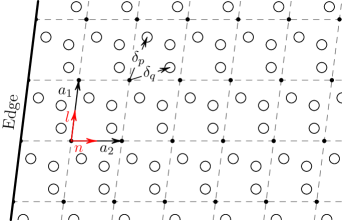
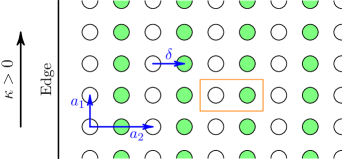
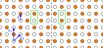
Both bulk Verba et al. (2012a) and edge Lisenkov et al. (2014) collective spin wave excitations were considered previously in the arrays having a single dot in a primitive cell. Below, we will develop an analytical model for a periodic lattice with a non-trivial primitive cell containing several identical magnetic nanodots (having several sublattices), as shown in Fig. 1. For this purpose we introduce a multi-vector notation, which will allow us to significantly simplify the theoretical formalism for the case of arrays having multiple magnetic dots in a primitive cell and, basically, to formally reduce it to the well-developed formalism describing dynamics in arrays with a simple primitive cellLisenkov et al. (2014).
The lattice of the array is defined by the primitive vectors and , and the primitive cell consists of identical dots. Relative positions of the dots inside the primitive cell are defined by a set of vectors , defined in the local coordinate system of the cell, see Fig. 1. The static and dynamic magnetization of the dots in the cell are defined as and , and the modulus of the effective static field is denoted as , where is the index of a cell and denotes an individual dot inside the -th cell.
Using the -enumeration of the dots, equation (13) takes the following form:
| (15) |
where
| (16) |
and . Unfortunately, this representation is rather cumbersome and restricts further analysis, as it obscures the structure of the problem.
To simplify equation (15) we introduce a multi-vector of the length as:
| (17) |
Analogously, we introduce multi-vectors for the static components of the magnetization . In the following the multi-vectors are used as ordinary vectors in all the vector-vector and vector-matrix operations. As we will see further, the multi-vector notation is rather convenient in both the analytical and numerical analysis. The algebra of the multi-vectors is briefly formulated in Appendix B.
Rewriting equation (15) by replacing the sum over with a formally written matrix-vector multiplication and by using the multi-vector notation (17), one can represent it in the following form:
| (18) |
where denote the cell index, and are the block-matrices defined as:
| (19) | |||
| (20) |
and . Here, the tensor is also represented by a block-matrix:
| (21) |
where and
| (22) |
The block-matrix describes the behavior and interactions of a whole primitive cell of the array in contrast to the tensor (defined by equation (11)), which describes the behavior of a single dot. The block-matrix is the projection of the block-matrix in the same sense as presented by equation (14).
Using the same procedure, one can rewrite the equation (9) for static magnetization in terms of multi-vector notation in the following form:
| (23) |
where the “components” of the multi-vector represent the external magnetic fields acting on the each dot in the -th cell.
III.2 Edge modes
In this section we consider collective spin wave excitations in a semi-infinite array. The array occupies a half-plane and has an edge parallel to one of the lattice primitive directions, see Fig.1. In this case the static magnetic properties of the array demonstrate a translation symmetry along one of the principal directions, but there is no translational symmetry along the other lattice direction. Using this arrangement, we will develop an analytical model to describe the collective spin wave excitation localized near the edges of a semi-infinite array of magnetic dots.
We define the position vector of -th cell as:
| (24) |
where and are the integers enumerating cells in the directions and , respectively (Fig. 1). The half-plane occupied by the array corresponds to , while the index can take any integer value.
Since the array has a translational symmetry along the direction, the static configuration of the magnetization depends only on the index :
| (25) |
and elementary spin wave solutions can be found in the form
| (26) |
where is the wave-number of the spin wave mode. Using these expressions in equation (18) yields the equation for the spin wave profile :
| (27) |
where
| (28) |
and
| (29) |
To compute the sum in (29) we introduce the Fourier transform of the cell mutual demagnetizing tensor:
| (30) |
Using the well-known “shift property” of the Fourier transform we obtain from (22):
| (31) |
Considering that is a real and symmetric tensor Beleggia et al. (2004) in the sense that , the Fourier image of the cell demagnetization block-matrix has the following symmetry properties:
| (32) |
Using the expression for the Fourier image (31) for equation (29) one gets:
| (33) |
where and are the reciprocal primitive vectors of the lattice and is the area of a unit cell. Using the well-known properties of the reciprocal primitive vectors and the identity , equation (33) can be simplified:
| (34) |
The analytical expressions for the Fourier image of the dot demagnetization tensor are known for all the practically interesting dot shapes (see equations (2.5)–(2.8) in [Verba et al., 2012a]). Therefore, equation (34) allows one to calculate the components of the block-matrix that are necessary for the solution of the equation (27).
In general, the block-matrix is not Hermitian and has no symmetry in respect to Hermitian conjugation. However, from the properties of the Fourier transform and the properties of the block-matrix in the equation (32) one can conclude that it has the following symmetry properties:
| (35) |
and
| (36) |
The static equation (23) can be rewritten in a similar way, considering that the static quantities (25) do not change in the direction of the vector :
| (37) |
Together, equations (27) and (37) are the central result of this paper. Using these equations one can calculate the distribution of the internal magnetic field ()in the array, equilibrium directions of the magnetic moments in each dot (), and the spectrum of collective spin wave edge excitations in a semi-infinite array of magnetic nanodots with a complex primitive cell.
Although equations (27) and (37) were obtained using purely analytical methods, further analytical solution of these equations (e.g., using the nearest neighbor approximation Bondarenko (2014)) is tedious and does not allow one to obtain qualitative analytical results in a closed form. The internal structure of the tensors is complicated, and, moreover, the dispersion equation (27) leads to a generalized eigenvalue problem with an infinite block “Toeplitz-like” matrix, in which blocks standing on the main diagonal are not equal, because when in (28).
Certain analytical results may be obtained in a rather artificial case when it is assumed that the internal magnetic field is uniform (in this case , which simplifies the solution of (27) considerably). However, even in this case the analytical calculation of the eigenvalues of the equation (27) with a non-Hermitian block Toeplitz matrix is non-trivial Tilli (1998), and the spectrum of collective spin wave excitations of the array may include distinct edge modes Lisenkov et al. (2014).
Therefore, in this paper we solve (27) and (37) numerically. The details of the numerical procedure are discussed in Sec.V. We would like to stress, that even for the numerical solution of the equation (27), the knowledge of the analytical structure of this equation provides significant advantages. For example, one can scale the results obtained numerically for relatively small systems for the case of much larger systems and can calculate spin wave damping and FMR absorption spectra without additional numerical analysis (see Sec. IV for further details).
Equations (27) and (37) were derived for a semi-infinite array of magnetic nanodots, but this specific geometry is only reflected in the range of summation over the index (, i.e., half-plane). The same equations with different summation ranges describe a number of other geometries, that are characterized by a translational symmetry along only one direction (). In particular, equations (27) and (37) with unrestricted should describe spin waves in an infinite array (see the next section). These equations, without any further modifications, can be used to describe the spin waves in a finite “stripe” () of a magnetic dot array, or the waves propagating along the internal “domain walls” in an infinite array. The latter example is considered in more details in Sec. VI.2. In all the following sections we shall not indicate explicitly the range of summation over the transversal indices (, ), assuming that they take physically relevant values in each particular case.
III.3 Bulk modes
In the previous section, we developed a model describing the dynamics of a magnetic dot array under the assumption that the array has a periodic translational symmetry along the vector , but that the translational symmetry is broken along the vector due to the existence of the array’s boundary. Nevertheless, the model should be valid for the cells located far from the boundary, where the edge effects are negligible. Here, we show, that for an infinite array (or for the cells located far from the boundary) our theory can be reduced to the previously developed theory of infinite arrays Verba et al. (2012a). Also we provide a link between the tensor and the fundamental tensor introduced earlier.
To consider the case of an infinite dot array we assume that the translational symmetry also holds in the direction parallel to the primitive vector , meaning that all the cells in the array are equal: , and for all . In this case we can introduce a wave-number describing the wave profile in the direction. Now, the solution can be found in the form:
| (38) |
Direct substitution of (38) into the dynamic equation (27) yields a simple equation:
| (39) |
which coincides with equation (3.32) from Ref. [Verba et al., 2012a], obtained for bulk spin wave modes in an infinite array of nanodots. Here is the total spin wave wave-vector:
| (40) |
The interaction matrix has the following form:
| (41) |
where the block-matrix (fundamental tensor of the array Verba et al. (2012a)) may be found as:
| (42) |
where represents the reciprocal lattice of the array. We can use expression (42) to relate the tensors and as:
| (43) |
This equation provides a way of computing the block-matrix from the array’s fundamental tensor by performing only a single Fourier transform.
Another consequence of (43) is that the solutions of the eigenvalue problem (27) always include solutions of (39), i.e., numerically obtained spectrum of (27) will also contain the bulk spectrum of an infinite array.
To distinguish the localized edge spin wave modes from the set of all the other solutions of the equation (27), the spin wave profile (distribution of the spin wave amplitude ) for each mode should be analyzed. Edge modes will have a stronger magnetization near the edge, while the profiles of the bulk modes do not decay into the depth of the array.
IV FMR excitation in confined arrays
IV.1 Stationary amplitudes of forced edge modes
The excitation and damping of collective spin waves in arrays of magnetic nanodots may be considered in terms of a standard perturbation theory. Perturbation theory was previously used for a finite array in [Verba et al., 2012a], however, that solution has a significant drawback, namely, it requires the information about the magnetization dynamics in each particular dot, which makes the computation in the case of arrays containing a significant number of dots ineffective and time consuming.
Let us, first, consider a semi-infinite array. As it was shown in the previous section, a semi-infinite array has two types of modes: bulk modes and edge modes. The edge modes are localized in the area near the edge of the array, while bulk modes exist throughout the array. From (27), one may easily obtain the following normalization conditions for the bulk spin wave modes:
| (44a) | |||
| and, likewise, for the edge modes: | |||
| (44b) | |||
Here the indices denote the bulk mode zones, while the indices denote the localized edge modes. The bulk and edge modes are orthogonal to each other in the sense of equation (44b).
The norm defined by equation (44a) is not practical for the numerical computations, as it cannot be obtained directly from numerical solutions of equation (27). If we neglect the influence of the boundary on the bulk modes Lisenkov et al. (2014) we can eliminate the summation along the row using the dependence (38) and come to a more practical expression:
| (44a*) |
where describes the directions of the magnetic moments in a primitive cell situated far from the edge. The norm can be directly calculated from the numerical solution of equation (39).
Both the damping and driving microwave fields may be included in (5) as small magnetic fields acting on each dot in the array:
| (45) |
First of all, we are interested in the excitation of spin wave modes of the array by a spatially uniform external magnetic field (). Thus the perturbative magnetic field can be written as:
| (46) |
where is the Gilbert damping constant, is the excitation frequency, and c.c. denotes a complex-conjugate.
In the case of a spatially uniform excitation only the edge modes with and the bulk modes with are effectively excited. This allows us to consider the solutions for (45) only for a single row of cells, as in Fig. 1. The solution for the perturbed equation (45) may be written as:
| (47) |
where and are the stationary amplitudes of edge and bulk modes, are the localized solutions of (27), and are the solutions of (39). To find the amplitudes of the excited modes, one should plug (47) into (45) and use the normalization conditions (44b) to separate the equation of motion into a set of equations for individual spin wave amplitudes. In the first approximation we can neglect all the terms that are non-linear in , and for the non-degenerate modes the stationary amplitude of each of the edge modes is given by
| (48) |
where ,
| (49) | ||||
For bulk modes the stationary amplitude is defined by the expression that is similar to (48), but with
| (50) | ||||
Here are the Gilbert damping rates for the corresponding spin wave modes, and represents the coupling coefficient between the spin wave mode and the spatially uniform external driving magnetic field.
IV.2 Power absorption of a finite polygon-shaped array
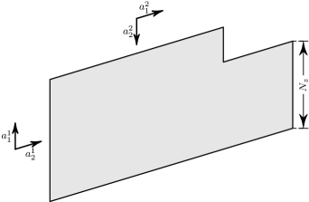
Now let us consider a finite array containing magnetic dots in the shape of a polygon. The polygon, shown in Fig. 2, has sides and each side () contains dots. The array is sufficiently large, so the edge modes traveling along the different faces may be treated as independent, and the bulk modes are unaffected by the edges of the array.
The total power absorbed by a finite array can be calculated as Gurevich and Melkov (1996):
| (51) |
where is a volume of a single dot.
Since the magnetization amplitude of the bulk modes is identical in each unit cell of the array, it can be found as:
| (52) |
Thus, the power absorbed (per unit cell) by the bulk modes is:
| (53) |
where
| (54) |
and .
The magnetization profiles of the localized edge modes are not uniform in a direction along which the translational symmetry is lacking. To calculate the absorption caused by the edge modes localized at each edge of the array, we choose one of the local primitive vectors () to be parallel to the chosen edge, as in Fig. 2. In this case we can calculate the power absorbed by a single row of primitive cells in the direction of the primitive vector :
| (55) |
where
| (56) |
and are the localized solutions of (27) for the set of primitive vectors and for .
Finally, the total absorption power of the array having number of cells may be calculated as:
| (57) |
This equation demonstrates that the influence of the edge modes fades away with increasing number of dots in the array as .
The tensors and defined by equations (54) and (56), respectively, have the form of effective partial susceptibility tensors for the bulk and edge modes at each particular edge. By analyzing eigenvectors of these tensors one may find certain polarizations of external microwave field that are necessary for a maximum or/and minimum absorption caused by a certain particular mode (see examples presented below for more detail). The ability to analytically calculate the macroscopic polarization properties of an array is not only useful for the engineering development of novel magnetic meta-materials, but also can provide a way to experimentally verify this theory.
A separate note should be made about the “corner modes” of the array, e.g., the spin wave modes localized near the vertices of an array of a finite size. Obviously, the power absorption caused by these modes does not depend on number of dots in the array, so their influence is smaller than the influence of the edge modes, and, in most practical cases, can be neglected.
Finally, if the array has spatial dimensions that are much larger than the wavelength of the driving microwave field, the edge effects become less important. However, if the tensor is known, one can calculate not only the absorbed microwave power, but also the reflection of electromagnetic waves from an array with an arbitrarily complex primitive cell using the approximate electrodynamic boundary conditions derived in [Lisenkov et al., 2015a].
V Peculiarities of numerical solution
To solve equations (27) and (37) numerically one should truncate the number of terms in the summation to some integer . Such a reduction of the initial problem for a semi-infinite array is equivalent to the problem of collective spin wave propagation in a finite stripe of magnetic nanodots. If the finite number of rows in a strip is sufficiently large, the edge spin wave modes localized at the opposite sides of the finite stripe will not interact with each other. Also, these edge modes may be degenerate (i.e. will have the identical values of the eigen-frequency () for certain value of wave-number ()). For arrays of dots having a perpendicular magnetic anisotropy the degeneracy occurs in the symmetry points of the Brillouin zone Lisenkov et al. (2014). In such a situation an eigenvalue solver returns vectors of the null space, which may be not localized near the opposite edges of the finite stripe, but the symmetric/antisymmetric combinations of such eigenmodes. In this case to analyze the “real” eigenmodes one should construct a linear combination of those combined modes which are localized at the desired edge.
The numerical solution of the truncated eigenvalue problem (27) gives a discrete set of eigen-frequencies and eigen-modes. To determine if a particular mode is localized near an edge, the profile of a given mode should be investigated. The numerical solution, however, cannot determine the number of localized modes, as when the truncation number increases, new localized modes may appear Landau and Lifshits (1977); Ivanov . However, since the main mechanism of the localization is the non-uniformity of an internal magnetic field Jorzick et al. (2002); Lisenkov et al. (2013, 2014) and since the magnetic field decreases as for the dots at the position away from the array edge, these new localized modes merge with the bulk spectrum and have no influence on magnetization dynamics of the array.
Equations (27) and (37) were written assuming that translational symmetry only holds along the direction of the primitive vector , while such a symmetry is lacking in the direction of . This absence of the translational symmetry may manifest itself not only at a physical edge of an array, but, also, at an internal boundary within the array, e.g., at a domain wall or at a peculiarity of the static magnetic field. For example, consider an internal boundary created by a domain wall with the following ground state distribution:
| (58) |
where and are the multi-vectors describing the stable states in the two domains separated by a domain wall. Using (58) in (27) and (37) it is possible to find a dispersion relation for the collective spin wave modes traveling along a domain wall in the array. Thus, using the above presented theory, one can calculate all the edge, domain wall, and bulk modes in a magnetic nanodot array. The analysis of the spatial profile of each of these modes will allow one to correctly distinguish bulk and domain-wall spin wave modes.
Truncating the summation range to , one could calculate the dispersion of spin wave modes in a stripe of dots containing a domain wall, but, it should be noted, that using such an approximation one may also introduce some “artifact” modes localized near the edges of the finite-size “stripe”. Taking the number to be sufficiently large ensures that the “artifact” modes do not interact with the domain wall modes, and by analyzing the spatial profiles of the different modes one can filter out all the “artifact” modes.
Of all the procedures required to obtain the numerical solution from the above presented theory, calculation of the numerical values of the block-tensor requires the most processing power, since the dipolar sum in (34) converges slowly. However, the convergence rate is different for different values of . Starting from a certain value only the elements of the sum with will be really significant. The exact value of depends on the dot shape and the interdot distance.
To compute the integral in (34), one may also use a fast Fourier transform (FFT) procedure or direct numerical integration, especially if only a few members of the sum are needed. Combining these techniques one can tune one’s computation procedure and optimize the time of computation.
The numerical values of the elements of the block-matrix depend only on the geometrical characteristics of the array (dot shape and lattice symmetry), and does not depend on the orientation of the static magnetization or on the direction of the external magnetic field. Thus, once computed, the value of may be saved, and, then, reused to calculate the array’s characteristics for different stable states and crystalline anisotropy values, drastically reducing computation time.
VI Examples
Below we consider several examples demonstrating applications of the above presented theory for different physical systems. We show that the developed theory can be used for the calculation of the collective spin wave spectra in rather complicated systems, which may be interesting for practical applications.
In all the following examples, we will consider arrays of dots that are have a shape of round cylinders with the radius and height . The static magnetic moments of all the dots are oriented perpendicular to the array plane. If the static magnetic moments of all the dots are oriented in the same direction (either or ), the static state will be called ferromagnetic (FM). If the magnetic moments of the nearest dots point in the opposite directions, the static magnetization state will be called antiferromagntic (AFM).
A computer program implementing the proposed theoretical formalism is available on the Internet Lisenkov et al. (2015c).
VI.1 Edge modes
VI.1.1 FMR excitation of a finite triangular array of magnetic nanodots in the FM static state
In this example we consider an FMR excitation of a finite array of magnetic nanodots. The dots are periodically arranged in the form of a right triangle, and have a square lattice with the lattice constant , as shown in Fig. 3. The array hs the following parameters: , , , , the number of dots along a leg of the triangle is , for a total of dots in the array. These particular parameters were chosen to guarantee the perpendicular stability of the FM state () and to ensure a significant dipolar interaction between the dots ().
The array considered in this example has the shape of a right triangle with three edges, two of which (the legs of the triangle) are equivalent and one is different (the hypotenuse). To employ the technique presented in Sec. IV we need to calculate collective spin wave spectra for two sets of the primitive lattice vectors:
| (59a) | |||
| for the modes localized near the legs and | |||
| (59b) | |||
| for the modes localized near the hypotenuse. | |||

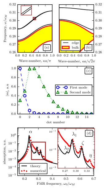
The dispersion relations for the legs of the triangle are shown in Fig. 4(a), while the dispersion for the hypotenuse is shown in Fig. 4(b). These relations were calculated numerically using equation (27) for equivalent stripes oriented along the primitive vectors defined by (59a) and (59b) with . The properties of the spin wave modes in an FM stripe of magnetic elements was previously investigated in detail in Lisenkov et al. (2014). For each stripe, it is important to note, that the FMR excitations can be localized along the stripe edges, and that these edge modes form pairs, localized on the opposite sides of the stripe. The edge modes in each pair are slightly split in frequency (see the inset in Fig. 4(a)), due to the symmetry breaking part of the dipole-dipole interaction Lisenkov et al. (2014), but the frequency splitting vanishes at the symmetry points of the Brillouin zone. Thus, to calculate the partial permeability tensors (56) one should take a linear combination of the eigenvectors of (27) in such a way that the high frequency components of the magnetization appear to be non-zero for dots located near one side of the stripe. For this particular configuration two well-separated edge modes are formed for the both sets of primitive vectors. The distribution of the high frequency components is plotted in Fig. 4(c) for the primitive vectors in (59a) for two edge modes with .
The FMR absorption spectrum of the array is plotted in Fig. 4(d) with a solid black line that corresponds to the results of the numerical solution of equation (57). As expected, the absorption spectrum consists of a main peak (marked with the symbol ) corresponding to bulk spin wave modes in the array, and several side-peaks associated with localized edge spin wave modes from the legs of the triangle (marked with and ) and from the hypotenuse (marked with ). The higher edge modes are less localized (see Fig. 4(c)), therefore these modes are less pronounced in the absorption spectrum, and the peak associated with the second mode localized on the hypotenuse is completely suppressed by the neighboring peaks.
When the number of the dot in the array is not large, it is possible to solve the Landau-Lifshitz equation (45) directly. Since we are interested only in the linear dynamics, we can linearize (45) using the same procedure as described in Sec. II:
| (60) |
The static properties can be found from (9), where the external field is absent in our case.
In Fig. 4(d) we also show (see red dotted line) the absorption spectrum found by the direct numerical solution of the linear inhomogeneous system of 1640 equations (60) for dots. It is evident, that the direct numerical simulation agrees reasonably well with our theory, as the frequencies and heights of the absorption peaks are in good quantitative agreement. The most notable difference between the theoretical and numerical simulations is the broadening of the bulk peak obtained in the direct numerical simulations. The direct numerical simulations also show an additional peak (marked by ) which does not correspond to any of the peaks obtained in the quasi-analytical theory.
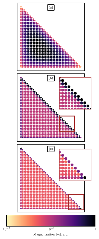
To further analyze the FMR absorption spectra and explain the differences between the theoretical and numerical values of the power absorption, we present in Fig. 5 the distribution of the microwave magnetization in the array for several values of the excitation frequency, calculated from (60). In Fig. 5(a) we plot the distribution of the magnetization at the central frequency of the bulk peak (marked with the an in Fig. 4 ). The distribution is not uniform across the array, especially at the vertexes. This non-uniform distribution is caused by a non-homogeneous internal magnetic field within the elements, and, in its turn, is causing inhomogeneous broadening of the main absorption peak Verba et al. (2012a) seen in Fig. 4(d).
The magnetization distribution for the hypotenuse mode (marked in Fig. 4 with a ) is plotted in Fig. 5(b) for the central frequency of the absorption peak. As one can see, most of the dots having the maximum values of the precession amplitude are localized near the hypotenuse, as theoretically predicted. The peak marked with the symbol in Fig. 4 is not present in the theoretical calculations. The distribution of magnetization at the central frequency of this peak is plotted in Fig. 5(c). For this case one can see, that the dots with the maximum amplitudes are situated at the vertexes of the triangle. These “corner modes” were neglected in (57), and they do not appear in the results obtained using the developed theory. The direct numerical simulation shows that although the influence of these “corner modes” is rather small, one should not completely neglect them for an array of this rather small size.
Overall, our theory gives results which correspond closely with direct numerical simulations, and provide a convenient way to analyze the features of the absorption spectra analytically. We would like to emphasize the computational advantage of our theoretical method. Each red dot in 4(d) required an independent solution of the inhomogeneous linear system of equations (60), having the arithmetic complexity of , making the direct numerical simulations impractical for large arrays of magnetic dots. Even for a system with only 820 dots, the time required to calculate the numerical absorption spectra was considerable. On the other hand, the theoretical line in the same figure, along with the dispersion relation in figure 4(a), can be almost instantaneously computed for an array of any size, independently of the number of dots. In other words, the arithmetic complexity of the quasi-analytical problem for the same array is of . Surely, this simple analytical technique cannot compete in numerical accuracy with the available micromagnetic packages Vansteenkiste et al. (2014), however, it can be useful for the approximate“engineering” of the desired absorption spectra with a subsequent quantitative verification using a computationally-intensive micromagnetic simulation.
VI.1.2 Nonreciprocal spin wave edge mode
This example is illustrating the non-reciprocal properties of the spin wave spectra in arrays of magnetic nanodots with complex unit cell. The non-reciprocity of a spin wave propagation is a desirable feature for the development of miniaturized and bias-free microwave isolators and circulators. Recently, non-reciprocal bulk collective spin wave modes have been investigated in detail for infinite arrays of magnetic nanopillars in Verba et al. (2013b). In particular, it was shown that for arrays of identical dots, non-reciprocal spin wave bulk modes only exist when the constituent elements have an out-of-plane magnetization. It was also shown that non-reciprocal spin waves bulk modes exist in infinite dot arrays with complex unit cells, e.g. containing two different types of dots . For example, the dots may have different values of the anisotropy field or different dot shapes, thus forming two different sub-lattices in the array.
In terms of the non-reciprocity the edge modes are not as restrictive as the bulk mores, and for the edge modes the necessary conditions for the non-reciprocal behavior could be lifted. For example, even a simple system of identical dots may have non-reciprocal edge modes Lisenkov et al. (2014). The general properties of the bulk spin wave spectra may be obtained by analyzing the symmetry properties of the fundamental tensor . For edge modes, however, an analytical solution is not possible, as the eigenvalue problem (27) is not symmetric. Nevertheless, much information can be gained by performing a numerical analysis based on (27) and (37).
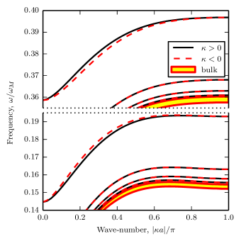
Here, we consider a semi-infinite array of magnetic nanodots having a rectangular lattice and a unit cell containing two different dot types, each having a different crystalline anisotropy within the same physical geometry (Fig. 7). Thus, each cell of the array consists of a heterogeneous pair of dots separated by the vector . To handle this problem in the framework of our theory the diagonal components of the demagnetization block-matrix (22) should rewritten in the following way :
| (61) |
where is a zero 3x3 matrix.
For this example, when performing the actual numerical calculations of the block-matrix using (29), it is convenient to separate the part of that corresponds to the crystalline anisotropy. Since the anisotropy tensors enters directly only into the multi-tensor , it is not necessary to recalculate the numerical values of for a different values of the anisotropy.
For the easy comparison with the previous results, we use the same geometrical parameters of the array as in Ref. [Verba et al., 2013b]: , , , . The unit cell consists of two dots, one magnetically isotropic and another having an out of plane easy axis crystalline anisotropy of the value of . It has been shown previously, that if = , the bulk spectrum is reciprocal. However, the edge modes in this case are not reciprocal. This is shown by the results of a numerical simulation plotted in Fig. 7. The numerical simulations of edge spin waves in the array were performed for the stripe of width cells.
In Fig. 7 we present the dispersion of the edge modes traveling along one side of the stripe. The spectrum consists of two zones of bulk waves and several well-separated edge modes for each zone. The mechanism of the edge mode formation is the same as in the case considered in Sec. VI.1.1, namely, a non-uniform static magnetic field near the edge of the array. Corresponding to the previous results, the bulk mode spectrum is reciprocal, while the spectrum of the edge modes is non-reciprocal, because the waves traveling in the opposite directions have different eigenfrequencies. The effect of the nonreciprocity is more pronounced for the modes that are separated from the bulk spectrum. However, the difference between the frequencies for the opposite values of is relatively small in this case.
The edge spin wave spectrum is reciprocal if the boundary in the array is made along the direction. The derivation of the exact analytical conditions of non-reciprocity for the spectrum of edge spin wave modes is beyond the scope of our current work and would be published elsewhere as a separate study.
VI.2 Domain walls
VI.2.1 Non-reciprocal spin waves traveling along domain walls in arrays in FM stable state
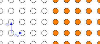
In the previous example the edge mode was well-separated in frequency from the bulk spectrum, and it exhibited a non-reciprocal behavior. While the non-reciprocity was present, the effect was relatively small. As it will be shown below, the non-reciprocal property of the spin wave modes propagating along the domain walls is substantially more pronounced than for the modes propagating along the array’s edges. The reason is that the non-reciprocal frequency splitting depends on the difference in ellipticity between the adjacent dots, and should be the most pronounced for the dots with the opposite directions of the static magnetic moments, and therefore, the opposite senses of the magnetization precession Verba et al. (2013b). Such a case is realized for an array in the FM stable state having a domain wall, which separates dots with anti-parallel directions of the magnetic moment, as is shown in Fig. 8.
Consider an infinite array, where the static magnetization(see (25)) has the following dependence of coordinate in the direction,:
| (62) |
where is a unit vector perpendicular to the array plane.
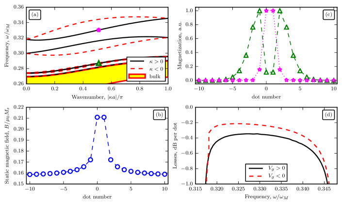
The dispersion relation for this array is shown in Fig. 9(a). The numerical simulations were performed for a stripe having rows. This number of rows was chosen to guarantee the absence of interaction between the domain-wall modes and the “artifact” edge modes (the “artifact” edge modes have been removed from the plot). The spectrum consists of the bulk modes, similar to the modes considered in Sec. VI.1.1, and the domain wall modes that are separated in frequency from the bulk modes. The mechanism responsible for the formation of the domain wall modes is a “potential well” formed by the non-uniform static magnetic field profile near the domain wall, as shown in Fig. 9(b). The domain-wall modes can be divided into two types: the modes localized directly on the domain wall and the modes localized near the domain wall, as shown in Fig. 9(c). The modes localized near the domain wall (green triangles in Fig. 9(c)) are similar to the modes formed near the edge of an array in FM stable state Lisenkov et al. (2014). The modes formed directly on the domain wall (magenta stars in Fig. 9(c)) exhibit a different behavior, as these modes are more localized and are highly non-reciprocal. In fact, these non-reciprocal modes still exist in a stripe of dots consisting of only two rows of dots with opposite directions of the static magnetization.
Non-reciprocal signal processing devices, such as isolators and circulators, allow propagation of waves in one direction and ado not allow such propagation in the opposite direction. This property is, typically, achieved due to the different insertion losses for waves traveling in the opposite directions.
Below, we demonstrate that such a nonreciprocal isolation effect can be achieved for the spin waves propagating along a domain wall in an array of magnetic nanodots.
The propagation losses of any of the spin wave modes caused by the magnetic damping can be calculated as:
| (63) |
where is the distance between the nearest dots and is the group velocity of the spin wave mode. The direction of the wave mode propagation (“forward” or “backward”) is determined by the sign of the group velocity.
It is clear from Fig. 9(a), that there is a small region near , where the spin wave mode marked by a magenta star in Fig. 9(a) has a negative group velocity , and, therefore, can be considered as a“backward-propagating” wave in this region.
The results of calculation of the propagation losses for spin wave modes forward- and backward-propagating along the domain wall using (63) are presented in Fig. 9(d). In contrast with the previous example, in this case the difference in losses between the forward- and backward-propagating wave modes is rather big (up to \ilu[0.2]\dBperdot), and is comparable to the direct insertion losses for the faster ( in our case) spin wave mode. This makes the non-reciprocal spin waves propagating allong the domain walls in the FM -state magnetic dot arrays rather interesting for practical realization of nano-sized microwave isolators.
VI.2.2 Spin wave domain wall modes in chessboard AFM stable state
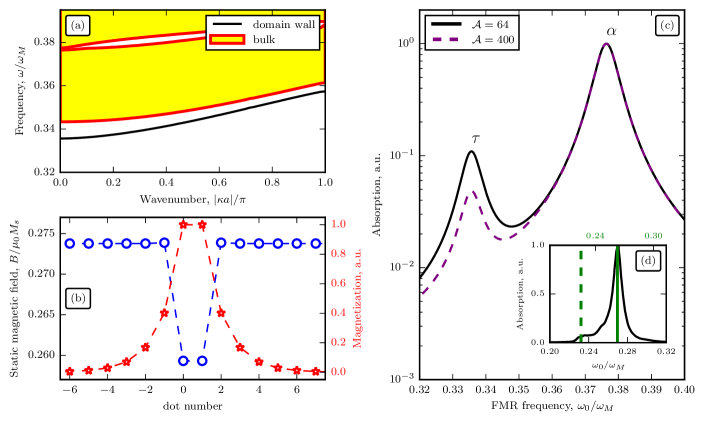
A magnetic dot array with a square lattice existing in the AFM static magnetization state, where the neighboring nanodots have opposite magnetization directions, has the lowest potential energy, and, therefore, forms a true ground state of the array. Such a state of the static magnetization, shown in Fig. 10 and having a zero net magnetic moment, is, usually, naturally formed during the demagnetization and is called the chessboard AFM (CAFM) stateBondarenko et al. (2011); Verba et al. (2012a). In reality, however, demagnetization does not lead to an ideal CAFM state Verba et al. (2013a), but, instead, it leads to the formation of clusters with local periodicity due to the spontaneous symmetry breaking between the two equivalent ground states of the array. A boundary between the two equivalent states CAFM states forms a “domain wall,” as shown in Fig. 10.
This example will explore the FMR (wave number equal to zero) absorption spectrum of the domain-wall modes in an array exising in a CAFM. To calculate the spin wave modes localized on the domain walls in the array we consider a single infinitely long domain wall within an infinite array, as shown in Fig. 10. The spectrum of the collective spin wave modes localized on the domain wall in the CAFM state is presented in Fig. 11(a). The spectrum consists of two bulk zonesVerba et al. (2012a) and a well-separated domain-wall mode. As in the previous example, we have removed the “artifact” modes caused by the specifics of the numerical solution (see Sec. V). The main reason for the modes localization on a domain wall is the variation of the internal magnetic field near the domain wall (see Fig. 11(b)). However, this variation is much smaller than in the example described in the previous section: only the dots that are the closest to the domain-wall have a distinct difference in their internal magnetic field, and this field variation is rather small, making the corresponding potential well rather shallow. Therefore, only a single localized mode appears in the spectrum of the array for the considered geometrical parameters, and the localization of this mode ir rather weak as shown in Fig. 11(b).
An array in the CAFM ground state does not have a net magnetic moment. Thus, its FMR absorption spectrum does not depend on the polarization of the external signal. In contrast, the contribution made by the external microwave field to the domain wall mode has a polarization dependence. If one takes the axis to be parallel to the domain wall, the partial susceptibility tensor (56) associated with the domain-wall modes has the following structure:
| (64) |
making the mode insensitive to the component of the external magnetic field that is perpendicular to the domain wall.
The difference in response of the bulk and edge modes is caused by the symmetry of the problem. In a domain existing in a uniform CAFM ground state, the magnetization in a particular dot will precess clockwise and counter-clockwise depending on the orientation of the magnetic moment of this dot Verba et al. (2012a), making a diagonal real tensor with .
However, in the case of domain-wall modes the boundary between the two CAFM ground states “synchronizes” the precession in the adjacent domains. The mirror symmetry of the problem requires that:
| (65a) | |||
| and | |||
| (65b) | |||
Using the above properties on can easily to show that:
| (66) |
Using Eq.(65) in (56) it is easy to get that . Analogously, one can show that , and, therefore, is the only non-zero component of the susceptibility tensor of the domain-wall spin wave mode.
A convenient characteristic of the final state of a demagnetized array Verba et al. (2013a) is the typical value of the number of dots forming a one CAFM cluster (cluster size). Thus, the total length (in dots) of a domain wall encircling all the clusters can be approximated as:
| (67) |
The full absorption power can be found from the expression that is analogous to (57):
| (68) |
where is the total absorption caused by the bulk modes, is the total absorption caused by the domain wall modes, and is the total absorption caused by the edge modes.
For sufficiently large arrays the role of the edge modes vanishes, although the absorption caused by the domain wall modes is inversely proportional to the size of a cluster in the array, and does not vanish in the limit . The absorption spectra calculated for two different values of the cluster size are shown in Fig. 11(c). The peaks associated with the bulk modes and domain-wall modes are marked with the symbols and , respectively. For the clusters containing dots these domain-wall modes may be clearly pronounced, producing an absorption that has a magnitude larger than 10% of the magnitude of the bulk mode peak. Thus, the absorption caused by the domain wall mode can be easily observed experimentally. Obviously, the static magnetization states with smaller clusters produce a larger absorption, however, when the linear dimensions of the domains get closer to the spin wave localization length (see Fig. 11(b)) the approximation of an infinitely long domain wall is no longer valid.
A previous work Verba et al. (2013a) calculated the FMR absorption spectrum for a CAFM array containing stable clusters using a micro-magnetic simulation. When the data from the micro-magnetic simulation is compared with our quasi-analytical theory, the results apper to be quite similar. These results are shown in Fig. 11(d), where the data taken from Ref. Verba et al., 2013a is shown by a continuous thin black line, while the vertical lines show the spectral positions of the absorption peaks calculated from our quasi-analytical. It is evident that the bulk peak obtained in the framework of our theory and shown by a solid vertical line, matches nicely with the absorption peak obtained from the micromagnetic simulations. Likewise, the dashed vertical line, which marks the absorption peak corresponding to the cluster of domain walls, matches well with the position of the plateau obtained in the micromagnetic simulations. Unfortunately, the data from Ref. Verba et al., 2013a was obtained for the cluster sizes of , for which the localized domain wall modes were not completely formed. That makes a more detailed quantitative comparison between the theory presented here and the micromagnetic simulations impossible. This is confirmed by the lack of a strong absorption peak corresponding to the domain wall modes in the micromagnetic simulations. The difference in the mode frequencies between the micromagnetic results and the analytical theory is caused, most likely, by the inhomogeneity of the internal magnetic field, the effect similar to the one described in Sec. VI.1.1.
Thus, the developed theory provides a reasonably good tool to estimate the cluster size from the FMR response measured or calculated for the arrays with sufficiently large clusters. However, for arrays with smallar clusters, the development of a technique capable of estimating the cluster size from the FMR response require a more rigorous estimation of the domains boundary length, than the one given by equation (67). A more rigorous estimation must take into account the “corner modes” that form at the domain wall intersections and the interactions between the domain-wall modes exsisting within one domain.
VII Conclusions
A general theoretical formalism, developed in this paper, allows one to calculate the following characteristics of the finite magnetic dot arrays having a complex primitive cell and a translational symmetry along one of the lattice vectors: (i) distribution of the internal magnetic field inside the array; (ii) equilibrium directions of the static part of the dot magnetization inside the array; (iii) spectra of the collective spin wave edge excitations in the array. We have shown that by introducing a “multi-vector” notation it is possible to reduce the solution of the Landau-Lifshitz equation for a dot array to a generalized eigenvalue problem. The components of the block-matrices involved in the eigenvalue problem for edge spin-wave excitations are obtained using a one-dimensional Fourier transform of analytically defined functions, which requires substantially less computation time than the typical micromagnetic simulations for the same system. Although only a macrospin approximation of the magnetization dynamics in a single dot is considered in this work, the developed formalism could be extended to describe the magnetization dynamics in the dot array with non-trivial distribution of the dynamic magnetization inside the dots (for one of possible extensions see Appendix A).
The above developed quasi-analytical approach made possible to develop a theory of the FMR excitation of finite dot arrays, taking into account the edge effects. It was also shown that, using the developed theory, it is possible to calculate the absorption spectra of finite dot arrays using much less computation effort than required for the direct micromagnetic simulations of a similar system. Moreover, the quasi-analytical representation of the partial magnetic susceptibility tensors provides a way to understand how each spin wave mode of the array interacts with the applied electromagnetic driving field.
We have also developed a computer program implementing our method Lisenkov et al. (2015c) and illustrated the application of the developed theory on the examples that fall into two categories: edge effects and domain-wall effects. In particular, it has been demonstrated that the FMR absorption spectrum calculated using our quasi-analytical theory for a finite array of magnetic nanodots having a shape of right triangle agrees very well with the results obtained by direct micromagnetic simulations. An example of an array with a complex elementary cell containing two different magnetic dots was also considered. It was demonstrated that such arrays, while having reciprocal spectrum of bulk spin wave modes, may have a non-reciprocal spectrum of the edge spin wave modes.
The spectra of spin wave excitations localized at the domain walls in arrays of magnetic nanodots were calculated for two cases: a domain wall between the two ferromagnetic static magnetization states and a domain wall between the two chessboard antiferromagnetic static magnetization states. In the first case, it was demonstrated that the modes localized on the domain-wall have a very high degree of non-reciprocity. The propagation losses for these modes appear to be significantly different for the opposite propagation directions, which can be used for the development of nano-sized microwave isolators and circulators. For the case of an array existing in a chessboard antiferromagnetic static magnetization state with domain walls (which is a natural state for a demagnetized array) it has been shown that the spin wave modes localized on the domain walls may produce a significant contribution to the FMR absorption spectra. In contrast to the spin wave modes localized at the array’s edges, that have been considered in previous examples, the contribution to the FMR response by the modes localized on the domain wall in the chessboard antiferromagnetic ground state depends on the size of the domains, providing a tool to estimate the size of the domains, and, therefore, the “quality” of the static magnetization state of the dot array.
Acknowledgements.
This work was supported by the the Center for NanoFerroic Devices (CNFD) and the Nanoelectronics Research Initiative (NRI), by the DARPA MTO/MESO grant “Coherent Information Transduction between Photons,Magnons, and Electric Charge Carriers”, by the U.S. Army Contract from TARDEC, RDECOM, and by the Grant No. 1305574 from the National Science Foundation of the USA. I.L. and S.N. acknowledge Russian Scientific Foundation, Grant #14-19-00760 for financial support. I.L. thanks Mr. Steven Louis for the proofreading of the manuscript.Appendix A An extension of the theory beyond the macrospin approximation
In the theory devolved above we used the same demagnetization tensor for static (9) and dynamic (10) equations. This approximation is correct, when the dots are assumed to be magnetized uniformly among their volume (“macrospin approximation”) and the crystalline anisotropy is uniaxial. Here we show, that the developed theory can be extended to cover more general situations.
We demonstrate below that the theory can be substantially generalized if we use different static and dynamic demagnetization tensors in (9) and (11):
| (9′) |
and
| (11′) |
where and are the static and dynamic demagnetization tensors found in each particular case. In all the equations of the above developed theoretical formalism the static and dynamic demagnetization enter independently, so it is easy to trace all the changes caused by using different demagnetization tensors for static and dynamic magnetization.
A.1 High-order crystalline anisotropy
A high-order crystalline anisotropy is usually rather weak, compared to the the uniaxial anisotropy of the magnetic material and the shape anisotropy of the magnetic sample. However, in some particular cases the high-order anisotropy can be qualitative important. For example, this happens when the shape and crystalline anisotropies are not present ( e.g. when magnetic elements are spherical and made of an isotropic material Gurevich and Melkov (1996); Kaczér and Murtinová (1974)) or when the shape and crystalline anisotropies cancel each other.
As an example of the high-order anisotropy here we consider the first-order cubic anisotropy. Let us assume that the energy of the cubic anisotropy is and the crystalline axes are: , and . The energy added by the first-order cubic anisotropy to the energy of a single magnetic dot can be written Stancil and Prabhakar (2009) as (here and below we drop the dot’s index):
| (69) |
where
| (70) |
Thus, the effective field caused by the anisotropy can be found as:
| (71) |
where
| (72) |
To linearize (71) we use expansion (6). In contrast with the uniaxial case, the static and dynamic magnetic fields are different. The static field can be found as:
| (73) |
while the dynamic field is found as:
| (74) |
with
| (75) |
Thus, the correction to the demagnetization tensor caused by the cubic anisotropy can be written as:
| (76) | |||
| (77) |
Note, that the effective demagnetization tensor now explicitly depends on the magnetic ground state of a dot. The dynamical equations do not get any additional complexity, however the static problem (9′) becomes considerably more complicated. Although, in a particular case, when the static component is aligned along one of the axes of the cubic anisotropy the correction to the demagnetization tensor has a simple form Stancil and Prabhakar (2009):
| (78) |
A.2 Dots with non-uniform dynamic magnetization
For the sake of simplicity we derived the above presented theory implying that the magnetic dots have a uniform magnetization profile. Nevertheless, the theory can be extended for the cases, when the spatial profile of the spin wave mode is not uniform. The straightforward extension is possible when: (i) the ground state of static magnetization of the dot is uniform; (ii) the interactions between the dots do not alter the ground state of a single dot, e.g. when the inter-dot interaction is weaker than the exchange and dipolar self-interactions in a single dot; and (iii) the eigenmodes of a dot are substantially separated in frequency. Under these assumptions, our approach remains sufficiently simple to allow the analytical analysis, and can describe dynamics of realistic experimental systems Kruglyak et al. (2010b); Tacchi et al. (2010, 2011).
Let us assume that we know from either a micromagnetic simulation Vansteenkiste et al. (2014); Buijnsters et al. (2014); Grimsditch et al. (2004) or from an analytical solution Jorzick et al. (2002); Grimsditch et al. (2004); Zivieri and Stamps (2006) the linear magnetization dynamics of a single isolated magnetic dot in a form:
| (79) |
where is the static magnetization component, is the vector mode profile of the -th spin wave mode and is the number of these spin wave modes. For simplicity we assume that the modes do not interact. It is convenient to switch to a temporary coordinate system (denoted by the symbol ′), in which , and write the distribution of the dynamic part of the magnetization in this system as Kalinikos and Slavin (1986):
| (80) |
where is a real dimensionless matrix-density:
| (81) |
The normalization coefficient is found from the condition:
| (82) |
where is the volume of the dot and the operator is defined in the same way as in (13).
Following the same procedure as in [Beleggia and De Graef, 2003], we obtain the Fourier representation of the effective demagnetization tensor:
| (83) |
where in the three-dimensional reciprocal vector and is:
| (84) |
After that, the effective dynamic demagnetization tensor and its in-plane Fourier image can be found straightforwardly Verba et al. (2012a):
| (85) |
Now one substitutes this tensor into (11′) and finds eigen-frequencies and spin-wave mode profiles of the collective spin-wave excitations in an array of interacting nanodots using (27). After that, the distribution of magnetization within a single dot for the -th array mode can be found for each dot in the array:
| (86) |
A case of multiple interacting modes within a dot can be considered introducing a new “layer” of multi-vectors, representing amplitudes of different modes, similarly to the approach used for a complex unit cell in this paper. The operators will, however, have to be renormalized, as the different modes may carry a different magnetic moment.
Appendix B Multi-vector algebra
“Multi-vectors” are introduced as the first rank objects in a multi-vector space. Instead of scalars for “ordinary” Euclidean vectors, each multi-vector () is an ordered collection of three-dimensional vectors . A multi-vector of the size contains three-dimensional vectors:
| (87) |
Below we define the algebra in the multi-vector space. First of all we define a bilinear operation (scalar product) of two multi-vectors of the size :
| (88) |
The second rank objects in the multi-vector space are the block-matrices by , each element of which is a 3 by 3 matrix of scalars. A product of a multi-vector and a block-matrix is defined as follows:
| (89) |
and returns another multi-vector. Although it is never used in the paper, one can also define scaling a multi-vector as a multiplication of a multi-vector by a scalar and other higher rank operations.
The multi-vectors are convent for analytical and numerical calculations. In computer algebra systems the operations (88) and (89) can be defined as custom user operations and one can analyze the object in the multi-vector space analytically.
For numerical simulations one can formally use multi-vectors as ordinary vectors of scalars of the size :
| (90) |
One can easily check, that the operations (88) and (89) remain valid in this case.
It is important to stress, that our notation for “multi-vectors” is not related to the “Multivector Calculus” described in Hestenes (1968).
References
- Demokritov and Slavin (2012) S. Demokritov and A. Slavin, Magnonics: From Fundamentals to Applications, Topics in Applied Physics (Springer, 2012).
- Krawczyk and Grundler (2014) M. Krawczyk and D. Grundler, J. Phys.: Condens. Matter 26, 123202 (2014).
- Nikitov et al. (2015) S. A. Nikitov, D. V. Kalyabin, I. V. Lisenkov, A. N. Slavin, Y. N. Barabanenkov, S. A. Osokin, A. V. Sadovnikov, E. N. Beginin, M. A. Morozova, Y. P. Sharaevsky, and et al., Uspekhi Fizicheskih Nauk 58 (2015), 10.3367/ufne.0185.201510m.1099.
- Kruglyak et al. (2010a) V. V. Kruglyak, S. O. Demokritov, and D. Grundler, J. Phys. D: Appl. Phys. 43, 264001 (2010a).
- Serga et al. (2010) A. A. Serga, A. V. Chumak, and B. Hillebrands, J. Phys. D: Appl. Phys. 43, 264002 (2010).
- Sinova and Zutic (2012) J. Sinova and I. Zutic, Nature Materials 11, 368–371 (2012).
- Xu et al. (2016) Y. Xu, D. D. Awschalom, and J. Nitta, eds., Handbook of Spintronics (Springer Science + Business Media, NY, 2016).
- Guslienko and Slavin (2000) K. Y. Guslienko and A. N. Slavin, Journal of Applied Physics 87, 6337 (2000).
- Jorzick et al. (2001) J. Jorzick, C. Krämer, S. O. Demokritov, B. Hillebrands, B. Bartenlian, C. Chappert, D. Decanini, F. Rousseaux, E. Cambril, E. Söndergard, and et al., Journal of Applied Physics 89, 7091 (2001).
- Gubbiotti et al. (2004) G. Gubbiotti, M. Conti, G. Carlotti, P. Candeloro, E. D. Fabrizio, K. Y. Guslienko, A. Andre, C. Bayer, and A. N. Slavin, J. Phys.: Condens. Matter 16, 7709–7721 (2004).
- Galkin et al. (2005) A. Galkin, B. Ivanov, and C. Zaspel, Journal of Magnetism and Magnetic Materials 286, 351–355 (2005).
- Tacchi et al. (2010) S. Tacchi, M. Madami, G. Gubbiotti, G. Carlotti, H. Tanigawa, T. Ono, and M. P. Kostylev, Phys. Rev. B 82, 024401 (2010).
- Tacchi et al. (2011) S. Tacchi, F. Montoncello, M. Madami, G. Gubbiotti, G. Carlotti, L. Giovannini, R. Zivieri, F. Nizzoli, S. Jain, A. O. Adeyeye, and et al., Physical Review Letters 107, 127204 (2011).
- Kruglyak et al. (2010b) V. V. Kruglyak, P. S. Keatley, A. Neudert, R. J. Hicken, J. R. Childress, and J. A. Katine, Physical Review Letters 104, 027201 (2010b).
- Bondarenko et al. (2010) P. V. Bondarenko, A. Y. Galkin, B. A. Ivanov, and C. E. Zaspel, Phys. Rev. B 81, 224415 (2010).
- Bondarenko et al. (2011) P. V. Bondarenko, A. Y. Galkin, and B. A. Ivanov, Journal of Experimental and Theoretical Physics 112, 986–1003 (2011).
- Huber and Grundler (2011) R. Huber and D. Grundler, Spintronics IV (2011), 10.1117/12.892168.
- Keatley et al. (2011) P. S. Keatley, V. V. Kruglyak, P. Gangmei, and R. J. Hicken, Philosophical Transactions of the Royal Society A: Mathematical, Physical and Engineering Sciences 369, 3115–3135 (2011).
- Verba et al. (2012a) R. Verba, G. Melkov, V. Tiberkevich, and A. Slavin, Physical Review B 85, 014427 (2012a).
- Verba et al. (2013a) R. Verba, V. Tiberkevich, K. Guslienko, G. Melkov, and A. Slavin, Physical Review B 87, 134419 (2013a).
- Verba et al. (2013b) R. Verba, V. Tiberkevich, E. Bankowski, T. Meitzler, G. Melkov, and A. Slavin, Applied Physics Letters 103, 082407 (2013b).
- Carlotti et al. (2014) G. Carlotti, G. Gubbiotti, M. Madami, S. Tacchi, F. Hartmann, M. Emmerling, M. Kamp, and L. Worschech, J. Phys. D: Appl. Phys. 47, 265001 (2014).
- Khymyn et al. (2014) R. Khymyn, V. Kireev, and B. A. Ivanov, Condens. Matter Phys. 17, 33701 (2014).
- Kakazei et al. (2015) G. N. Kakazei, X. M. Liu, J. Ding, V. O. Golub, O. Y. Salyuk, R. V. Verba, S. A. Bunyaev, and A. O. Adeyeye, Applied Physics Letters 107, 232402 (2015).
- Lisenkov et al. (2015a) I. Lisenkov, V. Tyberkevych, S. Nikitov, and A. Slavin, Applied Physics Letters 107, 082405 (2015a).
- Verba et al. (2012b) R. Verba, G. Melkov, V. Tiberkevich, and A. Slavin, Appl. Phys. Lett. 100, 192412 (2012b).
- Shaw et al. (2007) J. M. Shaw, W. H. Rippard, S. E. Russek, T. Reith, and C. M. Falco, Journal of Applied Physics 101, 023909 (2007).
- Wang et al. (2011) Y. Wang, F. Xiu, Y. Wang, J. Zou, W. P. Beyermann, Y. Zhou, and K. L. Wang, Nanoscale Research Letters 6, 134 (2011).
- Semenova et al. (2013) E. K. Semenova, F. Montoncello, S. Tacchi, G. Dürr, E. Sirotkin, E. Ahmad, M. Madami, G. Gubbiotti, S. Neusser, D. Grundler, and et al., Phys. Rev. B 87, 174432 (2013).
- Weller et al. (2000) D. Weller, A. Moser, L. Folks, M. Best, W. Lee, M. Toney, M. Schwickert, J.-U. Thiele, and M. Doerner, IEEE Trans. Magn. 36, 10–15 (2000).
- Schmool et al. (2008) D. Schmool, A. Apolinario, F. Casoli, and F. Albertini, IEEE Trans. Magn. 44, 3087–3090 (2008).
- Bandiera et al. (2012) S. Bandiera, R. C. Sousa, B. Rodmacq, and B. Dieny, Appl. Phys. Lett. 100, 142410 (2012).
- Pal et al. (2014) S. Pal, J. W. Klos, K. Das, O. Hellwig, P. Gruszecki, M. Krawczyk, and A. Barman, Appl. Phys. Lett. 105, 162408 (2014).
- Puszkarski (1973) H. Puszkarski, IEEE Trans. Magn. 9, 22–27 (1973).
- Jorzick et al. (2002) J. Jorzick, S. O. Demokritov, B. Hillebrands, M. Bailleul, C. Fermon, K. Y. Guslienko, A. N. Slavin, D. V. Berkov, and N. L. Gorn, Physical Review Letters 88, 047204 (2002).
- Lisenkov et al. (2013) I. Lisenkov, D. Kalyabin, and S. Nikitov, Appl. Phys. Lett. 103, 202402 (2013).
- Lisenkov et al. (2014) I. Lisenkov, V. Tyberkevych, A. Slavin, P. Bondarenko, B. A. Ivanov, E. Bankowski, T. Meitzler, and S. Nikitov, Phys. Rev. B 90, 104417 (2014).
- Shindou et al. (2013a) R. Shindou, R. Matsumoto, S. Murakami, and J.-i. Ohe, Physical Review B 87, 174427 (2013a).
- Shindou et al. (2013b) R. Shindou, J.-i. Ohe, R. Matsumoto, S. Murakami, and E. Saitoh, Physical Review B 87, 174402 (2013b).
- Chisnell et al. (2015) R. Chisnell, J. S. Helton, D. E. Freedman, D. K. Singh, R. I. Bewley, D. G. Nocera, and Y. S. Lee, Physical Review Letters 115, 147201 (2015).
- Kaczér and Murtinová (1974) J. Kaczér and L. Murtinová, Physica Status Solidi (a) 23, 79 (1974).
- Vasseur et al. (1996) J. O. Vasseur, L. Dobrzynski, B. Djafari-Rouhani, and H. Puszkarski, Physical Review B 54, 1043 (1996).
- Nikitov et al. (2001) S. Nikitov, P. Tailhades, and C. Tsai, Journal of Magnetism and Magnetic Materials 236, 320–330 (2001).
- Krawczyk and Puszkarski (2008) M. Krawczyk and H. Puszkarski, Physical Review B 77, 054437 (2008).
- Kostylev et al. (2008) M. Kostylev, P. Schrader, R. L. Stamps, G. Gubbiotti, G. Carlotti, A. O. Adeyeye, S. Goolaup, and N. Singh, Applied Physics Letters 92, 132504 (2008).
- Ho et al. (1990) K. M. Ho, C. T. Chan, and C. M. Soukoulis, Physical Review Letters 65, 3152 (1990).
- Kushwaha et al. (1993) M. S. Kushwaha, P. Halevi, L. Dobrzynski, and B. Djafari-Rouhani, Physical Review Letters 71, 2022 (1993).
- Grimsditch et al. (2004) M. Grimsditch, L. Giovannini, F. Montoncello, F. Nizzoli, G. K. Leaf, and H. G. Kaper, Physical Review B 70, 054409 (2004).
- Malago et al. (2015) P. Malago, L. Giovannini, R. Zivieri, P. Gruszecki, and M. Krawczyk, Physical Review B 92, 064416 (2015).
- Buijnsters et al. (2014) F. J. Buijnsters, A. Fasolino, and M. I. Katsnelson, Physical Review B 89, 174433 (2014).
- Kruglyak et al. (2006) V. V. Kruglyak, M. L. Sokolovskii, V. S. Tkachenko, and A. N. Kuchko, Journal of Applied Physics 99, 08C906 (2006).
- Urmancheev et al. (2016) R. Urmancheev, D. Kalyabin, and S. Nikitov, Journal of Magnetism and Magnetic Materials 401, 50–55 (2016).
- Klos et al. (2011) J. W. Klos, M. Krawczyk, and M. Sokolovskyy, Journal of Applied Physics 109, 07D311 (2011).
- Lisenkov et al. (2015b) I. Lisenkov, D. Kalyabin, S. Osokin, J. Klos, M. Krawczyk, and S. Nikitov, Journal of Magnetism and Magnetic Materials 378, 313–319 (2015b).
- Donahue and Porter (1999) M. Donahue and D. Porter, OOMMF User’s Guide, Version 1.0, Tech. Rep. Interagency Report NISTIR 6376 (National Institute of Standards and Technology, Gaithersburg, MD, 1999).
- Fischbacher et al. (2007) T. Fischbacher, M. Franchin, G. Bordignon, and H. Fangohr, IEEE Trans. Magn. 43, 2896–2898 (2007).
- Vansteenkiste et al. (2014) A. Vansteenkiste, J. Leliaert, M. Dvornik, M. Helsen, F. Garcia-Sanchez, and B. Van Waeyenberge, AIP Advances 4, 107133 (2014).
- Guslienko et al. (2008) K. Y. Guslienko, A. N. Slavin, V. Tiberkevich, and S.-K. Kim, Physical Review Letters 101, 247203 (2008).
- Beleggia and De Graef (2003) M. Beleggia and M. De Graef, Journal of Magnetism and Magnetic Materials 263, L1–L9 (2003).
- Beleggia et al. (2004) M. Beleggia, S. Tandon, Y. Zhu, and M. De Graef, Journal of Magnetism and Magnetic Materials 278, 270 (2004).
- Winter (1961) J. Winter, Phys. Rev. 124, 452–459 (1961).
- Borovik et al. (1977) A. E. Borovik, V. S. Kuleshov, V. A. Slyusarev, and M. A. Strzhemechnyǐ, Soviet Journal of Experimental and Theoretical Physics 46, 1229 (1977).
- Lisenkov et al. (2015c) I. Lisenkov, V. Tyberkevych, and A. Slavin, “MagDots: Magnetization dynamics of nanodot arrays,” https://github.com/ivlis/MagDots.git (2015c).
- Stancil and Prabhakar (2009) D. Stancil and A. Prabhakar, Spin Waves: Theory and Applications (Springer, London, 2009).
- Gurevich and Melkov (1996) A. G. Gurevich and G. A. Melkov, Magnetization, Oscillations and Waves (CRC PressINC, New York, 1996).
- Riley et al. (2006) K. Riley, P. Hobson, and S. Bence, Mathematical Methods for Physics and Engineering: A Comprehensive Guide (Cambridge University Press, 2006).
- Krivosik and Patton (2010) P. Krivosik and C. E. Patton, Phys. Rev. B 82, 184428 (2010).
- Bondarenko (2014) P. V. Bondarenko, Technical Physics Letters 40, 813–815 (2014).
- Tilli (1998) P. Tilli, Linear Algebra and its Applications 272, 59–89 (1998).
- Landau and Lifshits (1977) L. Landau and E. Lifshits, Quantum Mechanics: Non-relativistic Theory, Butterworth Heinemann (Butterworth-Heinemann, 1977).
- (71) B. A. Ivanov, personal communication.
- Zivieri and Stamps (2006) R. Zivieri and R. L. Stamps, Physical Review B 73, 144422 (2006).
- Kalinikos and Slavin (1986) B. A. Kalinikos and A. N. Slavin, Journal of Physics C: Solid State Physics 19, 7013–7033 (1986).
- Hestenes (1968) D. Hestenes, Journal of Mathematical Analysis and Applications 24, 313–325 (1968).