Chemodynamical modelling of the Milky Way

Abstract

Chemodynamical models of our Galaxy that have analytic Extended Distribution Functions (EDFs) are likely to play a key role in extracting science from surveys in the era of Gaia.

1 Introduction

Enormous observational resources are currently being expended on surveys of our Galaxy, and these expenditures will continue for at least the next five years. Consequently a major task of contemporary astronomy is to forge the resulting data into a coherent working model of our Galaxy. The community hopes to unravel the Galaxy’s assembly history, but such hopes will remain illusory until we have firmly established what’s out there: how is the Galaxy currently structured, and how is it working?

Given the extent to which a star’s chemistry must encode the time and place of its formation, and the way stellar kinematics encodes the Galaxy’s gravitational field and through that the Galaxy’s distribution of matter, chemodynamical models will be central to extracting science from surveys. The central role of chemodynamical models is further underlined by three issues:

• The contents of survey catalogues are strongly influenced by selection effects: catalogues are dominated by what’s near or luminous. It’s easier to account for selection effects by imposing them on mock observations of a model than to “correct” the observational data as was often done in the past.

• The majority of stars in any catalogue are close to the survey’s limiting magnitude or resolution. Consequently, observational errors are small for only a minority of surveyed stars. It is much easier to impose the observational errors on mock observations than to correct the data. The revolution in data gathering over the last couple of decades ensures that statistical errors are no longer the limiting source of uncertainty in scientific understanding; we are rather limited by incomplete understanding of observational errors (“systematic” errors).

• A good chemodynamical model summarises the knowledge we have gained from several different surveys, and indeed tests this knowledge by checking that conclusions we have drawn from different bodies of data are mutually consistent. In fact, our ultimate, essentially complete understanding of our Galaxy will be embodied in the final chemodynamical model, which we will come to identify with the Galaxy in the same way that in the 19th century our planet was identified with a school-room globe.

2 What models to use?

2.1 Cosmological models

Simulations of dark-matter clustering form the backbone of cosmology. The physics that goes into them is extremely simple, yet it took 15 years for the simulations to get the basic picture right. For the last 15 years the community has struggled with simulations that include gas and star formation. It is now clear that the majority of baryons reside in the intergalactic medium and without powerful feedback from star formation galaxies become too luminous and too spheroidal. The effectiveness of feedback must be connected to the near fractal structure of the ISM. Cosmological simulations won’t be able to resolve this structure in the foreseeable future, so the community is hunting for an “effective field theory” that describes that $\ga 10\,{\rm pc}$-scale impact of this unresolved structure. There is no guarantee that such an effective theory exists, and certainly we can’t use its results now. Consequently, we have no ability to compute the consequences of the precise initial conditions specified by the concordance cosmology. In short cosmological simulations lack predictive power.

It’s hard even to characterise a cosmological simulation: if the equations of motion are integrated for a few timesteps, the billions of numbers that specify it change while the model remains the same. It’s a totally non-trivial task to ask if two simulations differ materially, and if they do, in what way.

Cosmological simulations are computationally costly – one model typically requires years of CPU time. Consequently, there’s no realistic prospect of fitting them to observational data. From this it follows that the insights they provide, though possibly useful, are of an anecdotal nature.

2.2 Oxford models

If we are to fit models to data, it’s vital to minimise the number of parameters required to specify a model. Over 90% of the Galaxy’s matter is contained in unobserved dark matter and we have to constrain the distribution of this material through the effect its gravitational field has on stars and gas. This we can do only to the extent that the Galaxy is statistically stationary because any phase-space coordinates of stars are consistent with any gravitational potential $\Phi$ until you require that after a dynamical time has elapsed the system has not expanded or collapsed or otherwise changed its shape to a significant extent. Consequently, we focus on equilibrium Galaxy models. The Galaxy is not in exact equilibrium, but we hope to model non-equilibrium phenomena such as spiral structure and the warp by perturbing an equilibrium model.

By Jeans’ theorem the distribution function (df) of an equilibrium model can be taken to be a function $f(I_{1},\ldots)$ of the constants of stellar motion. Most orbits in typical axisymmetric potentials are quasiperiodic in the sense that Fourier decomposition of the time series $x(t)$ obtained by numerical integration of the equations of motion contains power only at discrete frequencies $\omega$ that can be expressed as integer linear combinations $\omega=n_{1}\Omega_{1}+n_{2}\Omega_{2}+n_{3}\Omega_{3}$ of three fundamental frequencies $\Omega_{i}$. This fact guarantees the existence of angle-action coordinates $({\mathchoice{\hbox{{\gkvecten\char 18\relax}}}{\hbox{{\gkvecten\char 18\relax}}}{\hbox{{\gkvecseven\char 18\relax}}}{\hbox{{\gkvecseven\char 18\relax}}}},{\bf J})$, which are such that the actions $J_{i}$ are constants of motion and $\theta_{i}$ increases linear with time: $\theta_{i}(t)=\theta_{i}(0)+\Omega_{i}t$

The action $J_{r}$ quantifies excursions in $r$, the action $J_{\phi}$ is simply the component $L_{z}$ of angular momentum about the Galaxy’s symmetry axis, and the action $J_{z}$ quantifies motion perpendicular to the Galactic plane. In Oxford we have developed techniques for computing transformations between action-angle and ordinary $({\bf x},{\bf v})$ coordinates (Binney 2012a; Sanders & Binney 2014, 2015a). Our techniques are by no means optimal and we continue to refine them. But they work and allow us to fit data to models defined by dfs $f({\bf J})$.

3 Distribution functions

We think of galaxies as sums of “components” or “populations”. Any non-negative function $f({\bf J})$ defines an equilibrium dynamical model of a component. A huge advantage of making the df  depend on the actions rather than energy $E$ is that then adding components is straightforward: you simply add the corresponding functions of ${\bf J}$

$$f({\bf J})=\sum_{i}f_{i}({\bf J}).$$ (1)

By contrast, if $E$ is permitted to be an argument of $f$, the system (if any) generated by the summed df  is in no useful sense the sum of its components because the presence of one component affects the energy scale of all components, just as it does the energy of a circular orbit of radius $R_{0}$. Moreover, finding the potential $\Phi$ that self-consistently corresponds to a df  $f({\bf J})$ is easy (Binney 2014) but hard when $E$ is an argument of $f$ (e.g Prendergast & Tomer 1970).

3.1 DF for thin and thick discs

We use the df

$$f_{\sigma}({\bf J})={\Sigma\Omega\nu\over 2\pi^{2}\sigma_{r}^{2}\sigma_{z}^{2}\kappa}[1+\tanh(J_{\phi}/L_{0})]{\rm e}^{-\kappa J_{r}^{2}/\sigma_{r}^{2}-\nu J_{z}/\sigma_{z}^{2}}$$ (2)

of a “quasi-isothermal” disc as the building block from which to assemble realistic models of the Galactic disc(s). In this df  $\Omega(J_{\phi})$ is the angular frequency of the circular orbit with angular momentum $J_{\phi}$, while $\kappa(J_{\phi})$ and $\nu(J_{\phi})$ are the radial and vertical epicycle frequencies of this orbit. $\Sigma$ also depends on $J_{\phi}$ and is to a good approximation the surface density at the radius $R_{\rm c}(J_{\phi})$ of the circular orbit. The choice $\Sigma=\Sigma_{0}{\rm e}^{-R_{\rm c}/R_{\rm d}}$ gives rise to a nearly exponential disc. The functions $\sigma_{r}(J_{\phi})$ and $\sigma_{z}(J_{\phi})$ control the radial and vertical velocity dispersions within the disc. A disc with roughly radius-independent scale height is obtained by taking $\sigma_{0}\propto{\rm e}^{-R_{\rm c}/R_{\sigma}}$ with $R_{\sigma}\simeq 2R_{\rm d}$. The purpose of the tanh function in eqn (2) is to eliminate counter-rotating orbits. For this purpose, $L_{0}$ should not be bigger than the typical angular momentum of a star in the bulge/bar. We typically adopt $L_{0}=10\,{\rm kpc}\,{\rm km}\,{\rm s}^{-1}$.

To date we have assumed that the thick disc can be adequately described by a single quasi-isothermal. This assumption is surely too crude, but so are the currently available data for the thick disc.

We take the df  of the thin disc to be a superposition of quasi-isothermals, one for the stars of each age. Specifically

$$f_{\rm thn}(J_{r},J_{z},L_{z})=\int_{0}^{\tau_{m}}{\rm d}\tau\,\Gamma(\tau)f_{\sigma_{\tau}}({\bf J}),$$ (3)

where

$$\Gamma(\tau)={{\rm e}^{\tau/t_{0}}\over t_{0}({\rm e}^{\tau_{m}/t_{0}}-1)}$$ (4)

encodes the history of star formation and the velocity-dispersion functions increase with age:

$$\begin{split}\sigma_{r}(J_{\phi},\tau)&=\sigma_{r0}\left({\tau+\tau_{1}\over\tau_{\rm m}+\tau_{1}}\right)^{\beta_{r}}{\rm e}^{(R_{0}-R_{\rm c})/R_{\sigma}}\cr\sigma_{z}(J_{\phi},\tau)&=\sigma_{z0}\left({\tau+\tau_{1}\over\tau_{\rm m}+\tau_{1}}\right)^{\beta_{z}}{\rm e}^{(R_{0}-R_{\rm c})/R_{\sigma}}.\end{split}$$ (5)

We typically adopt $\beta_{r}=0.33$ and $\beta_{z}=0.4$ so the velocity dispersions of a cohort increase rapidly at first and slower later on. $\tau_{\rm m}\simeq 10\,{\rm Gyr}$ is the age of the thin disc, and $\tau_{1}$ is chosen such that the velocity dispersion of stars at birth is $\sim 7\,{\rm km}\,{\rm s}^{-1}$. With these choices one obtains a disc in which the youngest stars are confined to a very thin disc in which the radial and vertical velocity dispersions are small, and the oldest stars form a thicker disc in which stars move on more eccentric orbits.

3.2 DF for stellar and dark halo

Posti et al. (2015) showed that self-consistent systems very similar to the Hernquist, NFW and Jaffe spheres can be generated by particular instances of the df

$$f({\bf J})={M_{0}\over J_{0}^{3}}{[1+J_{0}/h({\bf J})]^{(6-\alpha)/(4-\alpha)]}\over[1+g({\bf J})/J_{0}]^{2\beta-3}}.$$ (6)

Here $h({\bf J})$ and $g({\bf J})$ are homogeneous functions of degree one, i.e., $h(\gamma{\bf J})=\gamma h({\bf J})$, etc. For $|{\bf J}|\ll J_{0}$ $h$ dominates $f$ so $h$ controls the central structure of the resulting model. For $|{\bf J}|\gg J_{0}$, $g$ dominates $f$, so $g$ controls the structure of the model’s halo. By varying the way $h$ and $g$ depend on the individual components of ${\bf J}$, the model can be made prolate or oblate and its velocity distribution can be made tangentially or radially biased. We take the dfs of the stellar and dark halos to be instances of the df (6).

4 Metallicity-blind models

Binney (2010, 2012b) examined models defined by a disc df  and a specified gravitational potential that was a sum of the contributions from a double-exponential stellar disc, a gas disc, and simple spheroidal models of the bulge and the dark halo. A success of this work was that it indicated that the accepted value of the azimuthal component $V$ of the solar velocity with respect to the Local Standard of Rest was many sigma too small. Schönrich et al. (2010) subsequently explained how the metallicity gradient in the disc led Dehnen & Binney (1998) to extract an erroneous value of $V$ from the Hipparchos data.

Binney (2012b) had fitted the disc df  to the Geneva-Copenhagen survey (GCS: Nordström et al. 2004; Holmberg et al. 2009), which contains only nearby stars ($s\la 120\,{\rm pc})$. Binney & et al. (2014) compared the predictions of this df  for the contents of the RAVE survey (Steinmetz & et al. 2006; Kordopatis & et al. 2013), which extends to $s\ga 2\,{\rm kpc}$. The predictions for $v_{z}$ were extremely successful. Those for $v_{R}$ and $v_{\phi}$ quite successful, but far from the plane the df  predicted values of $\sigma_{R}$ that were too small. Given the small contribution that the thick disc makes to the GCS, these shortcomings in the predictions for RAVE were to be expected. Piffl & et al. (2014) fitted the dfs of the disc and stellar halo to the RAVE data and showed that excellent fits could be obtained.

In the work just described the potential was generated by analytic models of the Galaxy’s components rather than by the mass distributions predicted by the df. Piffl et al. (2015) computed the observable properties of the model produced by the df of Piffl & et al. (2014) when the dark matter was also predicted by a df rather than a specified density distribution. The chosen halo df was the one that in isolation generates the density distribution that Piffl & et al. (2014) adopted for the dark halo. When this same df is used to evaluate the density of dark matter in the presence of the disc, the dark halo is more centrally concentrated than Piffl & et al. (2014) assumed. Consequently, the self-consistent model that Piffl et al. (2015) recovered had a circular-speed curve that exceeded observational limits at $R\la 4\,{\rm kpc}$.

Binney & Piffl (2015) investigated whether this failure could be avoided by modifying the dfs of the disc and dark halo. They found that a model could be found that satisfied all the observational constraints considered by Piffl & et al. (2014) but the model generates too little optical depth to microlensing of bulge stars. The core problem is that an adiabatically compressed dark halo is too centrally concentrated. If such a dark halo is to contribute to the circular speed at $R_{0}$ to the required extent, it will contribute excessively to the rotation curve at $R\sim 3\,{\rm kpc}$. This is the first clear observational indication that the Galaxy’s baryons have not accumulated adiabatically.

5 Extended DFs

In all the above work the df  was fitted to catalogues without regard for the selection function. That is, the catalogue was taken to define a complete population that could be consistently described by a df. Actually, the population picked up by a survey at small distances differs from that selected at large distances because the nearby stars includes stars of low luminosity that will not be picked up at greater distances.

To model surveys with significant depth consistently, the model has to take cognisance of the factors that determine stellar luminosity and colour: mass, age, and metallicity. The dfs introduced by Binney (2010) recognised mass to the extent that a universal IMF was implicitly assumed, and age featured explicitly. But in comparing the resulting predictions with data this information was only used in a very simplistic way. Sanders & Binney (2015b, hereafter SB15b) took a significant step forward by extending the df  to include metallicity [Fe/H] and in comparisons with data used isochrones to exploit properly the information inherent in mass, age and metallicity. When metallicity features in the df, we say that the model has an edf  for Extended df.

SB15b derived a form for the Galaxy’s edf  by constructing analytic approximations to distributions that arise in the detailed chemodynamical models of Schönrich & Binney (2009). A time $\tau$ in the past the iron abundance $F\equiv\hbox{[Fe/H]}$ of the ISM at radius $R$ is taken to be

$$F(R,\tau)=F_{\rm m}+\left[F(R)-F_{\rm m}\tanh\left({\tau_{\rm m}-\tau\over\tau_{\rm F}}\right)\right],$$ (7)

where $\tau_{\rm m}\simeq 12\,{\rm Gyr}$, $\tau_{\rm F}\simeq 3\,{\rm Gyr}$ and

$$F(R)=\left(1-\exp\left[{-F_{R}(R-R_{\rm F})\over F_{\rm m}}\right]\right)F_{\rm m}.$$ (8)

According to these formulae, the abundance rises at a given radius from a pre-enrichment level $F_{\rm m}$ to its current value $F(R)$ on a short timescale $\tau_{\rm F}$. $R_{\rm F}$ is the radius at which [Fe/H] now vanishes, so $R_{\rm F}\simeq R_{0}$. For $R\simeq R_{\rm F}$ the argument of the exponential in eqn (8) is small, and expanding the exponential we see that $F_{\rm R}$ is the metallicity gradient at $R_{\rm F}$. Consequently, it is negative. It follows that $F_{\rm m}$ is the current iron abundance far from the Galactic centre. Once $R_{\rm F}$, $F_{\rm m}$ and $F_{\rm F}$ have been chosen, the iron abundance at the Galactic centre is determined.

SB15b took the age distribution of thin-disc stars to be

$$\Gamma(\tau)={1\over G_{0}}\exp\left({\tau\over\tau_{\rm f}}-{\tau_{\rm s}\over\tau_{\rm m}-\tau}\right).$$ (9)

When $\tau$ is only slightly smaller than the age $\tau_{\rm m}$ of the Galaxy, the second term in the exponential is large, so the star-formation rate is small. So at early times the SFR rises rapidly. It peaks and then declines as the first term in the exponential takes over. Our work with plain dfs relied on the first term in the exponential, thus an SFR that always decreases. As soon as we tried to fit the local metallicity distribution, we found it essential to add the second term, which encodes an early rise in the SFR to a peak about $2\,{\rm Gyr}$ after the Galaxy started to form.

Given the metallicity of stars born at each time and radius, the density $f({\bf J},\tau,F)$ of stars with given actions age and metallicity would follow if one had the Green’s function of the equation

$${\partial f\over\partial t}={\partial\over\partial{\bf J}}\cdot\left(-{\bf D}^{(1)}f+{\bf D}^{(2)}\cdot{\partial f\over\partial{\bf J}}\right)$$ (10)

that governs the diffusion of stars through action space. Here ${\bf D}^{(1)}$ and ${\bf D}^{(2)}$ are the first- and second-order diffusion coefficients. A suitable Ansatz for the Green’s function for diffusion in $J_{\phi}$ is

$$G(J_{\phi},J_{\phi}^{\prime},t)=\sqrt{{\tau_{\rm m}/t\over 2\pi\sigma^{2}_{L0}}}\exp\left[-{(J_{\phi}-J_{\phi}^{\prime}-D_{\phi}^{(1)}t)^{2}\over 2\sigma^{2}_{L0}t/\tau_{\rm m}}\right],$$ (11)

where $\sigma_{L0}$ is a constant related to the magnitude of $D_{\phi\phi}^{(2)}$. Since the angular momentum of the entire disc does not change as stars diffuse in angular momentum, we require $\int{\rm d}^{3}{\bf J}\,J_{\phi}(\partial f/\partial t)=0$, which implies that

$$D_{\phi}^{(1)}=-{\sigma_{L0}^{2}\over 2\tau_{\rm m}V_{c}R_{\rm d}}.$$ (12)

 

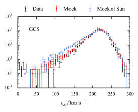
Figure 1: The fit to GCS data provided by the edf. Black points show the data, and red points the fit obtained. The pale blue points show the predictions of the edf  when no account is taken of the selection bias of the GCS.

 

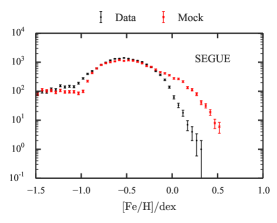
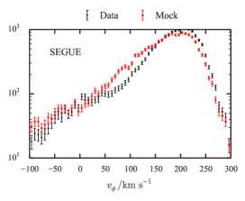
Figure 2: Predictions of the edf  for the statistics of G dwarfs from SEGUE. Black points show the data, and red points the predictions.

The red points in Fig. 1 show two of the excellent fits to the GCS catalogue (black points) that we obtain using this edf. The only statistically significant defect is a slight under-prediction of the number of stars with $v_{z}>50\,{\rm km}\,{\rm s}^{-1}$. This defect might reflect a poor choice of Galaxy potential. Since the parameters of the df  were adjusted to ensure that the stellar density profile $\rho(z)$ above the Sun agreed with the data points of Gilmore & Reid (1983), if our potential under-estimates the vertical force $K_{z}$, the distribution in $v_{z}$ that it provides will be too narrow.

The fit calls for the thin disc to have a significantly longer scalelength $R_{\rm d}=3.45\,{\rm kpc}$ than that of the thick disc, $R_{\rm d}=2.31\,{\rm kpc}$. The local metallicity gradient is $F_{\rm R}=-0.064\,\hbox{dex}\,{\rm kpc}^{-1}$ and the timescale of metallicity increase is $\tau_{\rm F}=3.2\,{\rm Gyr}$. The early star-formation timescale is $\tau_{s}=0.43\,{\rm Gyr}$, and the timescale of subsequent decay is $\tau_{\rm f}=8\,{\rm Gyr}$.

The pale blue points in Fig. 1 show the predictions of the edf when the selection function is set to unity. Then the edf  predicts increased numbers of stars with low [Fe/H] on eccentric orbits (which imply low $v_{\phi}$ and high $v_{R}$). The actual selection function is biased towards young stars, which tend to have higher metallicities and more circular orbits. In earlier work we, in effect, adjusted the df  to make the blue points coincide with the data. Consequently, we then derived values of the velocity-dispersion parameters $\sigma_{r0}$ and $\sigma_{z0}$ that are too small. Specifically, fitting with the proper selection function yields $(\sigma_{r0},\sigma_{z0})=(48.3,30.7)\,{\rm km}\,{\rm s}^{-1}$ for the thin disc, and $(50.5,51.3)\,{\rm km}\,{\rm s}^{-1}$ for the thick disc, whereas using the same potential but neglecting the selection function, Binney (2012b) obtained $(42.2,20.3)$ for the thin disc and $(26.3,34.0)\,{\rm km}\,{\rm s}^{-1}$ for the thick disc.

It’s interesting to compare the predictions of the edf fitted to the GCS with data for much more distant G-dwarfs from the SEGUE survey (Ahn & et al. 2014). The red points in Fig. 2 show these predictions. The main problem is that the model predicts more stars with $\hbox{[Fe/H]}>0$ than the data show. We suspect the problem lies with the observed metallicities rather than the model.

6 Conclusion

Models with analytic dfs $f({\bf J},\hbox{Fe/H})$ can provide remarkably good fits to current data and we argue are the key to extracting a coherent picture of our Galaxy from survey data. Including [Fe/H] in the df  enables one to handle selection functions, and doing so is very important. The EDF we use is inspired by an evolutionary scenario but it is a valid description of the present-day Galaxy regardless of the truth of the scenario. Conversely, the success of the EDF does not establish the validity of the scenario.

References

- Ahn & et al. (2014) Ahn C. P., et al. 2014, ApJS, 211, 17
- Binney (2010) Binney J., 2010, MNRAS, 401, 2318
- Binney (2012a) Binney J., 2012a, MNRAS, 426, 1324
- Binney (2012b) Binney J., 2012b, MNRAS, 426, 1328
- Binney (2014) Binney J., 2014, MNRAS, 440, 787
- Binney & et al. (2014) Binney J., et al. 2014, MNRAS, 439, 1231
- Binney & Piffl (2015) Binney J., Piffl T., 2015, ArXiv e-prints
- Dehnen & Binney (1998) Dehnen W., Binney J. J., 1998, MNRAS, 298, 387
- Gilmore & Reid (1983) Gilmore G., Reid N., 1983, MNRAS, 202, 1025
- Holmberg et al. (2009) Holmberg J., Nordström B., Andersen J., 2009, A&A, 501, 941
- Kordopatis & et al. (2013) Kordopatis G., et al. 2013, AJ, 146, 134
- Nordström et al. (2004) Nordström B., Mayor M., Andersen J., Holmberg J., Pont F., Jørgensen B. R., Olsen E. H., Udry S., Mowlavi N., 2004, A&A, 418, 989
- Piffl & et al. (2014) Piffl T., et al. 2014, MNRAS, 445, 3133
- Piffl et al. (2015) Piffl T., Penoyre Z., Binney J., 2015, MNRAS, 451, 639
- Posti et al. (2015) Posti L., Binney J., Nipoti C., Ciotti L., 2015, MNRAS, 447, 3060
- Prendergast & Tomer (1970) Prendergast K. H., Tomer E., 1970, AJ, 75, 674
- Sanders & Binney (2014) Sanders J. L., Binney J., 2014, MNRAS, 441, 3284
- Sanders & Binney (2015a) Sanders J. L., Binney J., 2015a, MNRAS, 447, 2479
- Sanders & Binney (2015b) Sanders J. L., Binney J., 2015b, MNRAS, 449, 3479
- Schönrich & Binney (2009) Schönrich R., Binney J., 2009, MNRAS, 396, 203
- Schönrich et al. (2010) Schönrich R., Binney J., Dehnen W., 2010, MNRAS, 403, 1829
- Steinmetz & et al. (2006) Steinmetz M., et al. 2006, AJ, 132, 1645