An analysis of the factors affecting keypoint stability in scale-space

Abstract

The most popular image matching algorithm SIFT, introduced by D. Lowe a decade ago, has proven to be sufficiently scale invariant to be used in numerous applications. In practice, however, scale invariance may be weakened by various sources of error inherent to the SIFT implementation affecting the stability and accuracy of keypoint detection. The density of the sampling of the Gaussian scale-space and the level of blur in the input image are two of these sources. This article presents a numerical analysis of their impact on the extracted keypoints stability. Such an analysis has both methodological and practical implications, on how to compare feature detectors and on how to improve SIFT. We show that even with a significantly oversampled scale-space numerical errors prevent from achieving perfect stability. Usual strategies to filter out unstable detections are shown to be inefficient. We also prove that the effect of the error in the assumption on the initial blur is asymmetric and that the method is strongly degraded in presence of aliasing or without a correct assumption on the camera blur.

1 Introduction

SIFT [1, 2] is a popular image matching method extensively used in image processing and computer vision applications. SIFT relies on the extraction of keypoints and the computation of local invariant feature descriptors. The scale invariance property is crucial. The matching of SIFT features is used in various applications such as image stitching [3], 3d reconstruction [4] and camera calibration [5].

SIFT was proved to be theoretically scale invariant [6]. Indeed, SIFT keypoints are covariant, being the extrema of the image Gaussian scale-space [7, 8]. In practice, however, the computation of the SIFT keypoints is affected in many ways, which in turn limits the scale invariance.

The literature on SIFT focuses on variants, alternatives and accelerations [3, 9, 10, 11, 12, 13, 14, 15, 16, 17, 18, 19, 20, 21, 22, 23, 24, 25, 26, 27, 28, 29, 30, 31, 32, 33]. A majority of them use the scale-space keypoints as defined in the SIFT method. The huge amount of citations of SIFT indicates that it has become a standard and a reference in many applications. In contrast, there are almost no articles discussing the scale-space settings in the SIFT method and trying to compare SIFT with itself. By this comparison we mean the question of comparing the scale invariance claim in SIFT with its empirical invariance, and the influence of the SIFT scale-space and keypoint detection parameters on its own performance. On this strict subject D. Lowe’s paper [2] remains the principal reference, and it seems that very few of its claims on the parameter choices of the method have undergone a serious scrutiny. This paper intends to fill in the gap for the main claim of the SIFT method, namely the scale invariance of its keypoint detector, and incidentally on its translation invariance. This is investigated by means of a strict image simulation framework allowing us to control the main image and scale-space sampling parameters: initial blur, scale and space sampling rates and noise level. We show that even in a particularly favorable scenario, many of the detected SIFT keypoints are instable. We prove that the scale-space sampling has an influence on the scale invariance and that finely sampling the Gaussian scale-space improves the detection of scale-space extrema. We quantify how the empirical invariance is affected by image aliasing and other errors due to wrong assumptions on the input image blur level.

Also, we verify the importance of the quadratic interpolation proposed in SIFT for refining the precision of the localized extrema. This is a fundamental step for the overall algorithm stability by filtering out unstable discrete extrema. On the other hand, we show that the contrast threshold proposed in SIFT is ineffective to remove the unstable detections.

Some of the conclusions of this paper were announced in [34]. The present article incorporates a more thorough rigorous analysis of the scale-space extrema and their stability. We reach this by separating the mathematical definition of the scale-space from the numerical implementation. We also add an analysis of the difference of Gaussians (DoG) scale-space operator and a discussion on how fine the scale-space should be sampled to fulfill the SIFT invariance claim.

The remainder of the paper is organized as follows. Section 2 presents the SIFT algorithm and details how to implement the Gaussian scale-space for the requirements of the present work. Section 3 exposes the SIFT theoretical scale invariance. With that aim in view, we explicit the camera model consistent with the SIFT method. Section 4 details how input images are simulated to be rigorously consistent with SIFT camera model. Section 5 explores the extraction of SIFT keypoints at each stage of the algorithm focusing on the impact of the scale-space sampling on detections. Section 6 looks at the impact of image aliasing and of errors in the estimation of camera blur. Section 7 is the conclusion.

2 The SIFT method and its exact implementation

In this section we briefly review the SIFT method and fix the adjustments that are required to make it ideally precise. This ideal SIFT will be used in the next sections to explore the limits of the SIFT method to detect scale-space extrema.

2.1 SIFT overview

SIFT derives from scale invariance properties of the Gaussian scale-space [7, 8]. The Gaussian scale-space of an initial image $u$ is the 3d function

$$v:(\sigma,{\bf x})\mapsto G_{\sigma}u({\bf x}),$$

where $G_{\sigma}u({\bf x})$ denotes the convolution of $u({\bf x})$ with a Gaussian kernel of standard deviation $\sigma>0$ (the scale). In this framework, the Gaussian kernel acts as an approximation of the optical blur introduced in the camera (represented by its point spread function). Among other important properties [8], the Gaussian approximation is convenient because it satisfies the semi-group property

$$G_{\sigma}G_{\gamma}u({\bf x})=G_{\sqrt{\sigma^{2}+\gamma^{2}}}u({\bf x}).$$ (1)

In particular, this permits to simulate distant snapshots from closer ones. Thus, the scale-space can be seen as a stack of images, each one corresponding to a different zoom factor. Matching two images with SIFT consists in matching keypoints extracted from these two stacks.

SIFT keypoints are defined as the 3d extrema of the difference of Gaussians (DoG) scale-space. Let $v$ be the Gaussian scale-space and $\kappa>1$, the DoG is the 3d function

$$w:(\sigma,{\bf x})\mapsto v(\kappa\sigma,{\bf x})-v(\sigma,{\bf x}).$$

When $\kappa\to 1$, the DoG operator acts as an approximation of the normalized Laplacian of the scale-space [2, 8],

$$v(\kappa\sigma,{\bf x})-v(\sigma,{\bf x})\approx(\kappa-1)\sigma^{2}\Delta v(\sigma,{\bf x}).$$

Continuous 3d extrema of the digital DoG are calculated in two successive steps. First, the DoG scale-space is scanned for localizing discrete extrema. This is done by comparing each voxel to its 26 neighbors. Since the location of the discrete extrema is constrained to the scale-space sampling grid, SIFT refines the position and scale of each candidate keypoint using a local interpolation model. Given a detected discrete extremum $(\sigma,{\bf x})$ of the digital DoG space, we denote by ${\bm{\omega}}_{\sigma,{\bf x}}({\bm{\alpha}})$ the quadratic function at sample point $(\sigma,{\bf x})$ given by

$${\bm{\omega}}_{\sigma,{\bf x}}({\bm{\alpha}})={\bf w}_{\sigma,{\bf x}}+{\bm{\alpha}}^{T}g_{\sigma,{\bf x}}+\frac{1}{2}{\bm{\alpha}}^{T}H_{\sigma,{\bf x}}{\bm{\alpha}},$$ (2)

where ${\bm{\alpha}}=(\alpha_{1},\alpha_{2},\alpha_{3})\in[-\nicefrac{{1}}{{2}},\nicefrac{{1}}{{2}}]^{3}$; $g_{\sigma,{\bf x}}$ and $H_{\sigma,{\bf x}}$ denote the 3d gradient and Hessian at $(\sigma,{\bf x})$ computed with a finite difference scheme. This quadratic function can be interpreted as an approximation of the second order Taylor expansion of the underlying continuous function (where its derivatives are approximated by finite differences).

To refine the position of a discrete extremum $(\sigma_{0},{\bf x}_{0})$ SIFT proceeds as follows.

1. Initialize $(\sigma,{\bf x})=(\sigma_{0},{\bf x}_{0})$.

2. Find the extrema of ${\bm{\omega}}_{\sigma,{\bf x}}$ by solving $\nabla{\bm{\omega}}_{\sigma,{\bf x}}({\bm{\alpha}})=0$. This yields ${\bm{\alpha}}^{\ast}=-\left(H_{\sigma,{\bf x}}\right)^{-1}\,g_{\sigma,{\bf x}}$ and a refined DoG value ${\bm{\omega}}_{\sigma,{\bf x}}({{\bm{\alpha}}}^{\ast})$. The corresponding keypoint coordinates are updated accordingly.

3. If $\|{\bm{\alpha}}^{\ast}\|_{\infty}<M_{\text{offset}}=0.6$ the extremum is accepted. Otherwise, go back to Step 1 and recompute the quadratic model at the closest point in the scale-space discrete grid.

This process is repeated up to $N_{\text{interp}}$ times (in SIFT, $N_{\text{interp}}=5$) or until the interpolation is validated. If after five iterations the result is not yet validated, the candidate keypoint is discarded.

Low contrast detections are filtered out by discarding keypoints with a small DoG value. Keypoints lying on edges are also discarded since their location is not precise due to their intrinsic translation invariant nature.

A reference keypoint orientation is computed based on the dominant gradient orientation in the keypoint surrounding. This orientation along with the keypoint coordinates are used to extract a covariant patch. Finally, the gradient orientation distribution in this patch is encoded into a $128$ elements feature, the so-called SIFT descriptor. We shall not discuss further the constitution of the descriptor and refer to the abundant literature [35, 30, 36, 17, 33, 18]. For a detailed description of the SIFT method we refer the reader to [37].

2.2 The Gaussian scale-space and its implementation

Let us assume that the input image has Gaussian blur level $c$. The construction of the digital scale-space begins with the computation of a seed image. For that purpose, the input image is oversampled by a factor $\nicefrac{{1}}{{{\delta_{\text{min}}}}}$ and filtered by a Gaussian kernel $G_{\sqrt{{\sigma_{\text{min}}}^{2}-c^{2}}}$ to reach the minimal level of blur ${\sigma_{\text{min}}}$ and inter-pixel distance ${\delta_{\text{min}}}$. The scale-space set is split into subsets where images share a common inter-pixel distance. Since in the original SIFT algorithm the sampling rate is iteratively decreased by a factor of two, these subsets are called octaves. We shall denote by $n_{\text{spo}}$ the number of scales per octave.

The subsequent images are computed iteratively from the seed image using the semi-group property (1) to simulate the blurs following a geometric progression

$$\sigma_{s}={\sigma_{\text{min}}}2^{s/{n_{\text{spo}}}},\quad s=1,\ldots,{n_{\text{spo}}}\!-\!1.$$

The digital Gaussian scale-space architecture is unequivocally defined by four parameters: the number of octaves $n_{\text{oct}}$, the minimal blur level $\sigma_{\text{min}}$ in the scale-space, the number of scales per octave $n_{\text{spo}}$ and the initial oversampling factor $\delta_{\text{min}}$. The standard values proposed in SIFT [1] are ${n_{\text{spo}}}=3$, ${\delta_{\text{min}}}=\nicefrac{{1}}{{2}}$ and $\sigma_{\text{min}}=0.8$. By increasing ${n_{\text{spo}}}$ the scale dimension can be sampled arbitrarily finely. In the same way by considering a small ${\delta_{\text{min}}}$ value, the 2d spatial position can be sampled finely.

From this digital Gaussian scale-space the difference of Gaussian scale-space (DoG) is computed. A DoG image at scale $\sigma$ is computed by subtracting from the image with blur level $\kappa\sigma$ the image with blur level $\sigma$ (with $\kappa>1$). Originally, the DoG scale-space is computed as a simple difference between two successive scales of the Gaussian scale-space so that $\kappa=2^{1/{n_{\text{spo}}}}$. In the present work, we have modified this definition by unlinking the parameters $\kappa$ and ${n_{\text{spo}}}$. This will allow us to better analyze the implications of the mathematical definition of the DoG operator (given by the $\kappa$-value) and the algorithmic implementation (given by the sampling parameter ${n_{\text{spo}}}$).

The Gaussian convolution implementation. The architecture of the Gaussian scale-space requires for the Gaussian convolution to be implemented so it satisfies the semi-group property (1). In SIFT, the Gaussian convolution is implemented as a discrete convolution with a sampled truncated Gaussian kernel. Such an implementation satisfies the semi-group property for the SIFT default parameters (${n_{\text{spo}}}=3$), but it fails for larger values of ${n_{\text{spo}}}$, as the level of blur to be added approaches zero.

To illustrate and quantify how the discrete Gaussian convolution fails to satisfy the semi-group property, we carried out the following experiment. A sampled Gaussian function of standard deviation $c=1.0$ was filtered $N=10$ times using a discrete Gaussian filter of standard deviation $\sigma$. If the Gaussian semigroup property were valid, then, applying $N$ times a Gaussian filter of parameter $\sigma$ should produce the same result as filtering only once with a Gaussian function of parameters $\sqrt{N}\sigma$. We fitted a Gaussian function to the filtered image by least squares. We compared the estimated standard deviation to the theoretical expected value $\sqrt{\sigma^{2}_{\text{in}}+N\sigma^{2}}$ (Figure 1 (a)). For low values of $\sigma$ (i.e., $\sigma<0.7$), the estimated blur deviates from the theoretical value $\sqrt{N}\sigma$ indicating that the method fails to satisfy the semi-group property. This is a direct consequence of image aliasing produced by excessive undersampling of the Gaussian kernel [38].

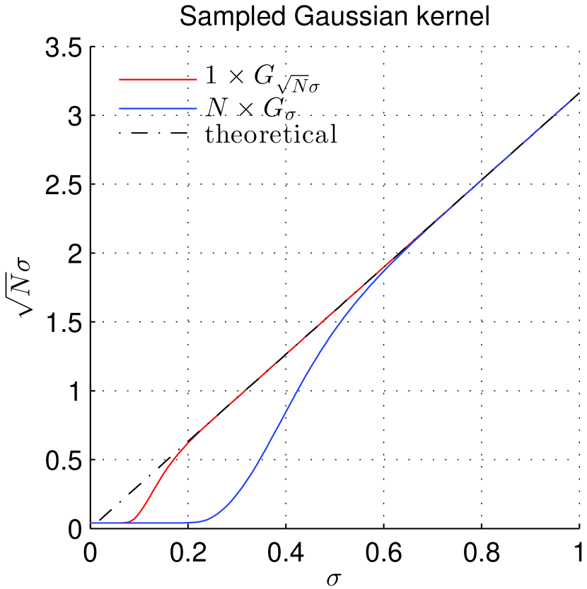
(a)

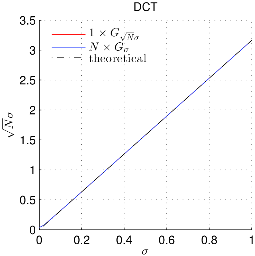
(b)

Figure 1: Analysis of the Gaussian convolution implementation through the semi-group property. An image having a Gaussian blob of standard deviation $c=1.1$ was filtered by (i) a Gaussian convolution of parameter $\sqrt{N}\sigma$, and (ii) by applying $N=10$ iterations of a Gaussian convolution of parameter $\sigma$ for different values of $\sigma$. Then the blur levels of the filtered images were estimated and compared to the theoretical expected value. (a) Discrete convolution with sampled Gaussian kernel. For low values of $\sigma$, the estimated blur deviates from the theoretical value $\sqrt{N}\sigma$. This is due to image aliasing when sampling the Gaussian kernel. (b) The DCT convolution fully satisfies the semi-group property.

To avoid this undesired phenomenon in our experiments that will consider strong scale oversampling, we replaced the discrete convolution by a Fourier-domain based convolution using the Discrete Cosine Transform (DCT). This can be interpreted as the continuous convolution between the DCT interpolation the discrete input image and the Gaussian kernel. The implementation details can be found in [38].

Figure 1(b) shows that the Fourier-based convolution satisfies the semi-group property even for low values of $\sigma$.

2.3 Building an ideal SIFT for parameter exploration

Since our goal was to explore extrema detection, we implemented an ideal SIFT where not only the convolution is exact, but also the extrema filters were turned off. The implementation of SIFT used in the present work differs from the original one on two aspects (besides the replacement of the discrete convolution by the Fourier-based one). First, SIFT proposes two filters to discard unreliable keypoints. The first one eliminates poorly contrasted extrema (those with low DoG value) and the second one discards extrema laying on edges (using a threshold on the local Hessian spectrum). These filters were deactivated to gain a full control of all detected extrema and to isolate the impact of each of them in terms of keypoints stability. This choice will be a posteriori justified, as we demonstrate in Section 5.3 that the DoG contrast threshold is inefficient.

Secondly, we decided to implement the DoG operator in such a way that the same mathematical definition is kept (i.e., using the same $\kappa$-value) regardless of the scale sampling rate ${n_{\text{spo}}}$. SIFT approximates the normalized Laplacian $\sigma^{2}\Delta$ by the difference of Gaussian operator. Different DoG definitions lead to different extrema. Consider for instance an image with a Gaussian blob of standard deviation $\sigma_{\text{blob}}$ as input. The normalized Laplacian will have an extremum at the center of the Gaussian blob, and scale $\sigma_{\text{detect}}=\sigma_{\text{blob}}$. On the other hand, the DoG scale-space of parameter $\kappa$ yields an extremum at scale $\sigma_{\text{detect}}=\nicefrac{{\sigma_{\text{blob}}}}{{\sqrt{\kappa}}}$. Consequently, the range of scales simulated in the scale-space is affected by the parameter $\kappa$.

For the requirements of the present work, and to investigate thoroughly how the operator definition affects extrema extraction, the considered DoG scale-space implementation allows us to set $\kappa$ and ${n_{\text{spo}}}$ independently.

Implementation details. The input image was oversampled by a factor $1/{\delta_{\text{min}}}$ to reach the ${\delta_{\text{min}}}$ sampling rate. This was done by using a cubic B-spline interpolation of order 3. From this interpolated image all images in the scale-space were computed using a combination of DCT Gaussian convolution and subsampling. For each scale $\sigma$ simulated in an octave, the algorithm computes two images, the first one corresponding to scale $\sigma$ and the second one corresponding to scale $\kappa\sigma$ (both being directly computed from the input image). Although we lost the benefit of a low computational cost, this gave us flexibility and allowed us to investigate the influence of the operator definition regardless of the scale-space sampling rate.

3 The theoretical scale invariance

In this section we give the correct proof that SIFT is scale invariant and stress the fact that this proof also indicates that knowing exactly the initial camera blur is crucial for the method’s consistency.

3.1 The camera model

In the SIFT framework, the camera point spread function is modeled by a Gaussian kernel $G_{c}$ and all digital images are frontal snapshots of an ideal planar object described by the infinite resolution image $u_{0}$. In the underlying SIFT invariance model, the camera is allowed to rotate around its optical axis, to take some distance, or to translate while keeping the same optical axis direction. All digital images can therefore be expressed as

$${\bf u}=:{\bf S}_{1}G_{c}H\mathcal{T}Ru_{0},$$ (3)

where ${\bf S}_{1}$ denotes the sampling operator, $H$ an arbitrary homothety, $\mathbf{\mathcal{T}}$ an arbitrary translation and $R$ an arbitrary rotation.

3.2 The SIFT method is theoretically invariant to zoom outs

It is not difficult to prove that SIFT is consistent with the camera model. Nevertheless, the proof in [6] is inexact, as pointed out in [39]. Let ${\bf u}_{\lambda}$ and ${\bf u}_{\mu}$ denote two digital snapshots of the scene $u_{0}$. More precisely,

$${\bf u}_{\lambda}={\bf S}_{1}G_{c}H_{\lambda}u_{0}\text{ \,\, and \, \, }{\bf u}_{\mu}={\bf S}_{1}G_{c}H_{\mu}u_{0}.$$ (4)

Assuming that the images are well sampled, namely that ${\bf S}_{1}$ is invertible by Shannon interpolation, and taking advantage of the semi-group property (1), the respective scale-spaces are

$$v_{\lambda}(\sigma,{\bf x}) = G_{\sqrt{\sigma^{2}-c^{2}}}{\bf I}_{1}{\bf S}_{1}G_{c}H_{\lambda}u_{0}({\bf x})=G_{\sigma}H_{\lambda}u_{0}({\bf x})$$ (5)

$$v_{\mu}(\sigma,{\bf x}) = G_{\sigma}H_{\mu}u_{0}({\bf x}),$$ (6)

where ${\bf I}_{1}$ denotes the Shannon interpolation operator. These formulae imply that both scale-spaces only differ by a reparameterization. Indeed, if $v_{0}$ denotes the Gaussian scale-space of the infinite resolution image $u_{0}$ (i.e., $v_{0}(\sigma,{\bf x})=G_{\sigma}u_{0}(\sigma,{\bf x})$) we have

$$v_{\lambda}(\sigma,{\bf x}) =H_{\lambda}(G_{\lambda\sigma}u_{0}({\bf x}))=v_{0}(\lambda\sigma,\lambda{\bf x}),$$ (7)

$$v_{\mu}(\sigma,{\bf x}) =v_{0}(\mu\sigma,\mu{\bf x}),$$ (8)

thanks to a commutation relation between homothety and convolution.

By a similar argument, the two respective DoG functions are related to the DoG function $w_{0}$ derived from $u_{0}$. For a ratio $\kappa>1$ we have

$$w_{\lambda}(\sigma,{\bf x}) =v_{\lambda}(\kappa\sigma,{\bf x})-v_{\lambda}(\sigma,{\bf x})$$ (9)

$$=v_{0}(\kappa\lambda\sigma,\lambda{\bf x})-v_{0}(\lambda\sigma,\lambda{\bf x})$$ (10)

$$=w_{0}(\lambda\sigma,\lambda{\bf x})$$ (11)

and similarly $w_{\mu}(\sigma,{\bf x})=w_{0}(\mu\sigma,\mu{\bf x})$.

Consider an extremum point $(\sigma_{0},{\bf x}_{0})$ of the DoG scale-space $w_{0}$. Then if $\sigma_{0}\geq\max(\lambda c,\mu c),$ this extremum corresponds to extrema $(\sigma_{1},{\bf x}_{1})$ and $(\sigma_{2},{\bf x}_{2})$ in $w_{\lambda}$ and $w_{\mu}$ respectively, satisfying $\sigma_{0}=\lambda\sigma_{1}=\mu\sigma_{2}.$ This equivalence of extrema between the two scale-space guarantees that the SIFT descriptors are identical.

Note that this same relation links the two normalized Laplacians applied on $v_{\lambda}$ and $v_{\mu}$, denoted respectively $nL_{\lambda}$ and $nL_{\mu}$, both related to the normalized Laplacian of $v_{0}$ denoted $nL_{0}$. We have

$$nL_{\lambda}(\sigma,{\bf x}) =\sigma^{2}\Delta v_{\lambda}(\sigma,{\bf x})$$ (12)

$$=(\lambda\sigma)^{2}\Delta v_{0}(\lambda\sigma,\lambda{\bf x})$$ (13)

$$=nL_{0}(\lambda\sigma,\lambda{\bf x})$$ (14)

$$nL_{\mu}(\sigma,{\bf x}) =nL_{0}(\mu\sigma,\mu{\bf x})$$ (15)

Therefore, considering extrema of the normalized Laplacian as keypoints will also lead to SIFT descriptors that are identical.

3.3 Knowing the camera blur is crucial for scale invariance

The knowledge of the camera blur is crucial to ensure the theoretical invariance to zoom-outs [39]. Indeed, DoG scale-spaces computed with a wrong camera blur have in general unrelated extrema. Starting again from the two digital snapshots ${\bf u}_{\lambda}$ and ${\bf u}_{\mu}$, but assuming a wrong blur $c^{\prime}$ instead of the correct blur $c$, the respective Gaussian scale-spaces are:

$$v_{\lambda}(\sigma,{\bf x}) =G_{\sqrt{\sigma^{2}-c^{\prime 2}}}{\bf I}_{1}{\bf S}_{1}G_{c}H_{\lambda}u_{0}({\bf x})$$ (16)

$$=G_{\sqrt{\sigma^{2}-c^{\prime 2}+c^{2}}}H_{\lambda}u_{0}({\bf x})$$ (17)

$$=v_{0}(\lambda\sqrt{\sigma^{2}-c^{\prime 2}+c^{2}},\lambda{\bf x})$$ (18)

and

$$v_{\mu}(\sigma,{\bf x}) =v_{0}(\mu\sqrt{\sigma^{2}-c^{\prime 2}+c^{2}},\mu{\bf x}).$$ (19)

We see that, because of the wrong blur assumption, the scale-space function $v_{0}$ is shrunken or dilated along scale. The corresponding DoG scale-spaces are:

$$\begin{split}w_{\lambda}(\sigma,{\bf x})&=v_{0}(\lambda\sqrt{\kappa^{2}\sigma^{2}-c^{\prime 2}+c^{2}},\lambda{\bf x})\\ &-v_{0}(\lambda\sqrt{\sigma^{2}-c^{\prime 2}+c^{2}},\lambda{\bf x}),\end{split}$$ (20)

$$\begin{split}w_{\mu}(\sigma,{\bf x})&=v_{0}(\mu\sqrt{\kappa^{2}\sigma^{2}-c^{\prime 2}+c^{2}},\mu{\bf x})\\ &-v_{0}(\mu\sqrt{\sigma^{2}-c^{\prime 2}+c^{2}},\mu{\bf x}).\end{split}$$ (21)

None of these are linear reparameterizations of the DoG function $w_{0}$ anymore. They yield therefore unrelated extrema. Such bias is maximal with detections at finer scales and with large zoom factors.

4 Simulating the digital camera

Controlling the image formation process permits us to measure how invariant SIFT is in different scenarios. Such a control was achieved by simulating images that are consistent with the SIFT camera model. Images at different zoom levels were simulated from a large reference real digital image $u_{\text{ref}}$ through Gaussian convolution and subsampling. To simulate a camera having a Gaussian blur level $c$, a Gaussian convolution of standard deviation $cS$, with $S>10$ was first applied to the reference image. The convolved image was then subsampled by a factor $S$. Assuming that the reference image has an intrinsic Gaussian blur level of $c_{\text{ref}}\ll cS$, the resulting Gaussian blur level is $\sqrt{c^{2}+(c_{\text{ref}}/S)^{2}}\approx c$. We estimated the blur level introduced by a digital reflex camera by fitting a Gaussian function to the estimated camera point-spread-function (following [40]). The obtained Gaussian blur levels varied from $c=0.35\text{--}0.95$, depending on the aperture of the lens (blur level increases with aperture size). Different zoomed-out and translated versions were simulated by adjusting the scale parameter $S$ and by translating the sampling grid. Thanks to the large subsampling factor, the generated images are noiseless. In addition, the images were stored with 32 bit precision to mitigate quantization effects. Figure 2 shows some examples of simulated images used in the experiments.

It might be objected that our simulations are highly unrealistic as the images to be compared by SIFT in a real scenario are not perfectly sampled or noiseless. Nevertheless, with an ever growing image resolution, more and more images will be compared by SIFT in large octaves, and therefore after a large subsampling, so that these properties can become realistic in practice. Furthermore, even if applying SIFT to the originals and regardless of initial noise and blur, the images at large scales also become anyway perfect so that the accuracy and repeatability issues under such favorable conditions are relevant.

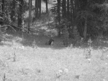
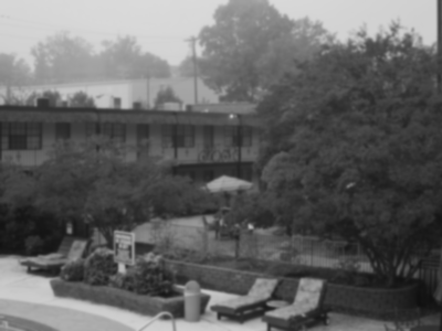
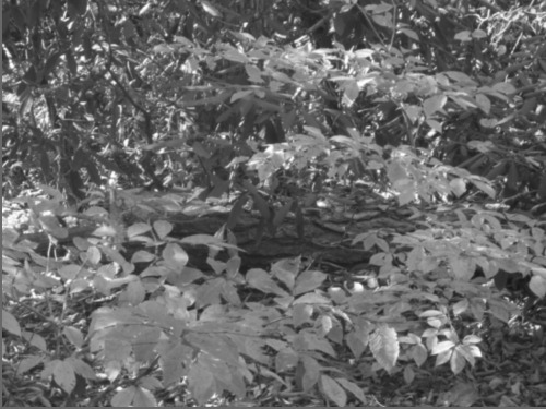
Figure 2: Examples of simulated images consistent with SIFT’s image camera model. The respective blur levels are $c=0.5$, $c=1.0$ and $c=0.6$.

5 Empirical analysis of the digital scale-space sampling

The SIFT method aims at locating accurately the extrema of the DoG scale-space. Ideally, one would like to detect and locate all extrema from the underlying continuous DoG scale-space. However, in practice, we do not have access to the continuous scale-space but to its discrete counterpart. In theory, as $\delta_{\text{min}}\to 0$ and ${n_{\text{spo}}}\to\infty$ the discrete scale-space better approximates the continuous scale-space therefore allowing to extract reliably all continuous extrema. This section investigates what happens when the sampling rates increase and how sampling affects the successive steps of the rudimentary procedure for detecting 3d scale-space discrete extrema, namely the extraction of discrete extrema, their quadratic interpolation and their filtering based on their DoG response.

To focus on the influence of the scale-space sampling, the study was carried out in the most favorable conditions: noiseless and aliasing-free input images ($c=1.1$ and $S=10$). In all experiments we set $\kappa=2^{1/3}$ to separate the mathematical definition of the DoG analysis operator from the scale-space discretization.

5.1 Number of detections

To evaluate how the scale-space sampling rates affects the number of detections we generated different scale-space discretizations by varying the parameters $({\delta_{\text{min}}},{n_{\text{spo}}})$, and extracted the 3d discrete extrema for each one of them.

Figure 3 (a) shows the number of detected extrema for the different scale-space samplings. At first sight, it seems that some digital scale-space samplings produce many more keypoints than the SIFT default sampling (${\delta_{\text{min}}}=\nicefrac{{1}}{{2}},{n_{\text{spo}}}=3$). However, this increase in detections happens for discretizations that are significantly unbalanced in space and in scale. By unbalance we mean that the scale and the space dimensions are sampled with very different sampling rates.

Boundary effect. To do a fair comparison of the different discrete detected extrema when changing the scale-space sampling rates, we have to consider that depending on the scale-space sampling, some extrema close to the lower scale boundary are not detected. Indeed, due to the scale discretization there are no detected keypoints with scale below ${\sigma_{\text{min}}}2^{1/2{n_{\text{spo}}}}$. To compensate for this dead range, which is a function of ${n_{\text{spo}}}$, we restricted the analysis to a common scale range independent of ${n_{\text{spo}}}$. This was achieved by discarding all extrema with scale below ${\sigma_{\text{min}}}2^{1/3}$. To avoid issues due to the coarse scale discretization, we used the keypoint scale obtained after refinement (2). Figure 3 (b) shows, for all scale-space tested configurations, the number of detections in the common scale region. The number of detected extrema lying in the common region is much more similar for all the scale-space samplings.

Duplicate detections. We will say that detections $(\sigma_{0},{\bf x}_{0})$ and $(\sigma_{1},{\bf x}_{1})$ are the same, if:

$$||{\bf x}_{0}-{\bf x}_{1}||_{\infty}\leq\epsilon\quad\text{and}\quad R^{-1}\leq\sigma_{1}/\sigma_{0}\leq R,$$ (22)

where $\epsilon$ and $R$ are the spatial tolerance and scale relative tolerance values respective.

Clearly, there is a compromise between saying that two detections are not the same and allowing some displacement due to numerical errors. Currently, we are not tackling the problem of precision but the problem of not mixing two different detections. With that aim, it seems reasonable that the tolerance values are set in order to avoid that one detection be mistaken for another. We opted to set tolerance values to $\epsilon=1.0$ and $R=2^{\nicefrac{{1}}{{2}}}$ independently of the scale-space sampling.

Let $\mathcal{D}$ be the set of detected DoG extrema. We call duplicates of $({\bf x}_{0},\sigma_{0})\in\mathcal{D}$ the subset of detected extrema $\text{D}({\bf x}_{0},\sigma_{0})\subset\mathcal{D}$ that satisfy (22). Given the set of all detected keypoints $\mathcal{D}$, we say that $\mathcal{U}$ is a representative set of unique detections if

$$\mathcal{U}=\operatorname*{arg\,min}|U|\quad\text{s.t.}\quad U\subset\mathcal{D}\,\,\text{and}\,\,\cup_{({\bf x},\sigma)\in U}D({\bf x},\sigma)=\mathcal{D},$$

where the number of keypoints in the set $U$ is denoted by $|U|$. Figure 3 (c) shows the number of unique detections in the common scale region. The number of unique detections is similar to the number of detections (Figure 3 (b)). This indicates that in general duplicate detections are negligible.

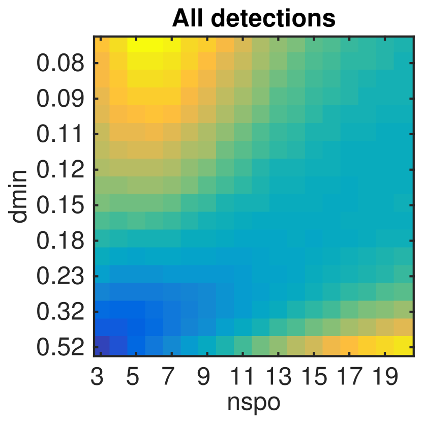
(a)

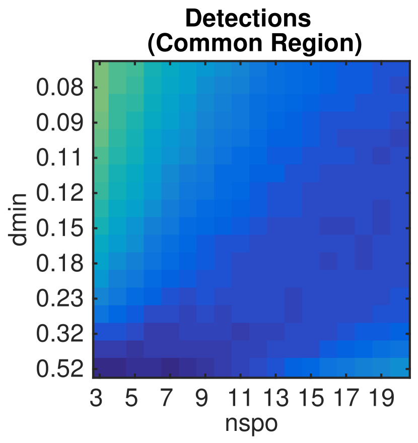
(b)

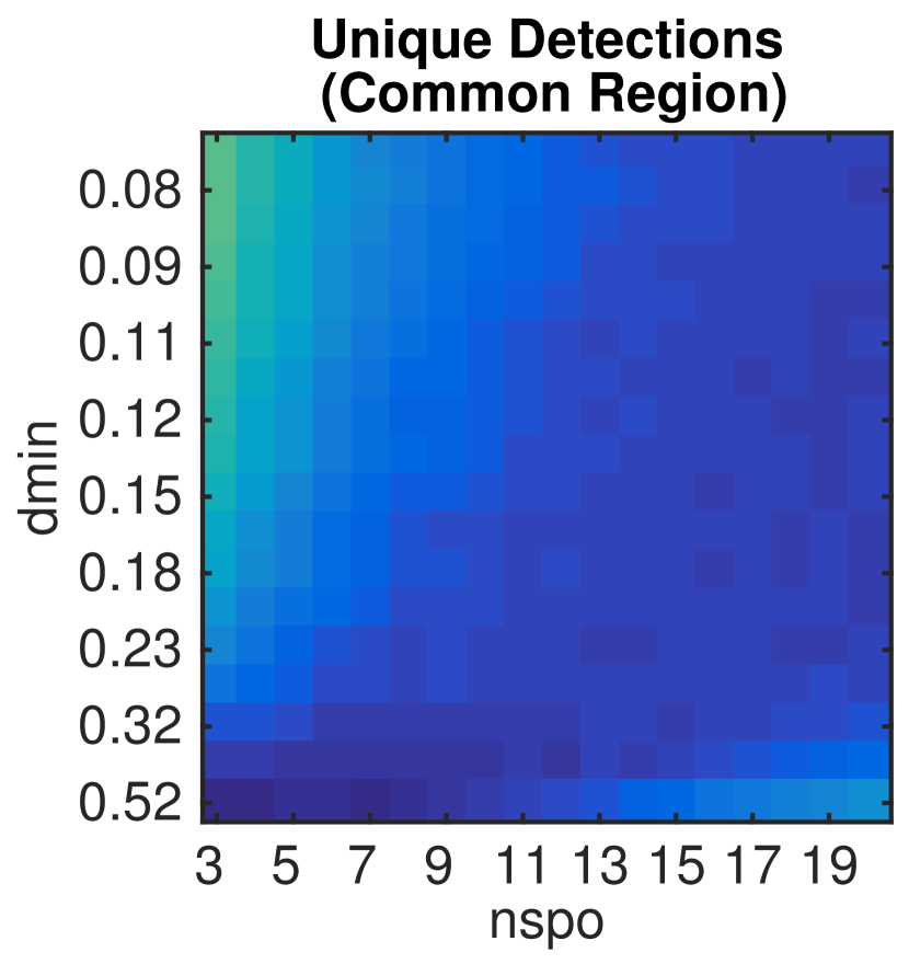
(c)

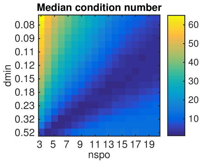
(d)

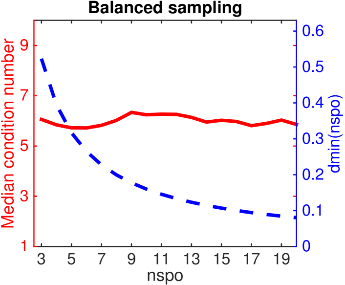
(e)

Figure 3: Influence of the scale-space sampling rate $({n_{\text{spo}}},{\delta_{\text{min}}})$ on the number of detected DoG extrema. (a) Number of 3d DoG discrete extrema. Unbalanced discretizations can produce twice as many detections as the default scale-space sampling used in SIFT (${n_{\text{spo}}}=3,{\delta_{\text{min}}}=\nicefrac{{1}}{{2}}$). This gap is reduced after compensating for a boundary effect by discarding 3d discrete extrema with detected scale below ${\sigma_{\text{min}}}2^{1/3}$ (b), and after removing duplicate detections (c). Unbalanced discretizations may lead to inaccurate local models for the extrema refinement proposed in SIFT. (d) Median of the condition numbers of DoG 3d Hessians used for extrema interpolations. Unbalanced sampling grids (shown in the top-right or bottom-left parts of this graph) produce extrema with significantly poor Hessian condition number. This leads to unstable extrema interpolations. (e) Balanced sampling rates (those satisfying (23), shown in the dotted blue line) lead to extrema having well conditioned Hessian matrices (red line).

Balancing the scale and space DoG sampling.

The SIFT algorithm proposes to refine the position of a discrete extremum using a quadratic interpolation. Having an unbalance sampling in scale and space may lead to an unreliable interpolation due to the very different discretization. As we presented in Section 2, the refinement of a keypoint is done by solving a linear system (from (2)). The sensitiveness to numerical errors can be measured by the linear system’s condition number (i.e., the condition number of the Hessian at the extrema to be refined). Figure 3 (d) shows the median of the condition number for the sets of detected extrema associated with different scale-space samplings. It shows that using a balanced sampling rate improves the overall stability of the extrema interpolation.

By balanced sampling we mean that the distance separating adjacent samples in the scale dimension is similar to the distance separating adjacent samples in space. For a DoG scale-space with parameter $\kappa$, the distance between the first two simulated scales is

$$\Delta\sigma=\kappa{\sigma_{\text{min}}}(2^{1/{n_{\text{spo}}}}-1).$$

Thus, to equally sample the Gaussian kernel

$$G({\bf x},\sigma)=\frac{1}{2\pi\sigma^{2}}e^{-||{\bf x}||^{2}/2\sigma^{2}}$$

in scale and space, the spatial inter pixel distance should be

$${\delta_{\text{min}}}=\sqrt{2}\Delta\sigma=\sqrt{2}\kappa{\sigma_{\text{min}}}(2^{1/{n_{\text{spo}}}}-1).$$ (23)

This relation between both sampling rates is plotted in Figure 3 (e) along with the median condition numbers on this set of balanced sampling rates. The condition number is mostly constant for balanced samplings.

5.2 Stability of DoG extrema to scale-space sampling

To evaluate if all 3d discrete extrema are equally stable to an increase of the DoG sampling rate, we simulated a set of increasingly dense balanced scale-spaces. We set the minimal scale-space blur level to ${\sigma_{\text{min}}}=1.1$. We simulated increasingly dense scale-space samplings $({n_{\text{spo}}},{\delta_{\text{min}}})_{i}$, for $i=1,\ldots,n$ with ${n_{\text{spo}}}=3,\ldots,19$ and the balanced spatial sampling rate ${\delta_{\text{min}}}:={\delta_{\text{min}}}({n_{\text{spo}}})$ given by (23) ($i=1$ being the coarsest one and $i=n$ the finest one). Figure 4 (a) shows that the number of detections is approximately constant for different balanced sampling rates.

Let $\mathcal{D}_{i}$ for $i=1\ldots,n$ be the sets of detected 3D extrema for the discretizations described above. Given a detected extremum $({\bf x}_{0},\sigma_{0})\in\mathcal{D}_{i}$, we say the extremum is detected in $\mathcal{D}_{j}$ if there exists $({\bf x},\sigma)\in\mathcal{D}_{j}$ such that they are the same detection according to the precision conditions (22). We say that a detected extremum $({\bf x}_{0},\sigma_{0})\in\mathcal{D}_{i}$ is new if it was not detected in $\mathcal{D}_{i-1}$. Given the sampling $i$, the rate of new extrema is computed as the proportion of new detected keypoints among the total number of detections. In the same way, we define the rate of lost extrema as the proportion of those present in the (coarser) sampling $i$ and not present in the (finer) sampling $i+1$. Figure 4 (b) shows the rate of new and lost detections as a function of the sampling rate. The new detection rate decreases with the sampling rate and stabilizes to a minimal rate of $10\%$ of the total number of detections for ${n_{\text{spo}}}\geq 14$. The same observations apply to the rate of lost extrema.

This surprising result means that despite sampling the scale-space very finely, 3d discrete extrema keep appearing and disappearing when changing the sampling.

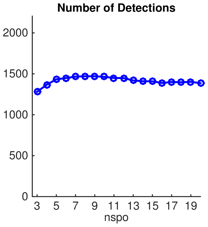
(a)

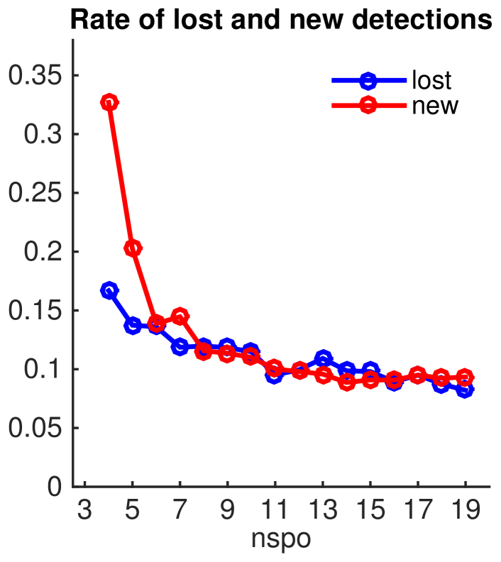
(b)

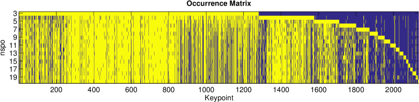
(c)

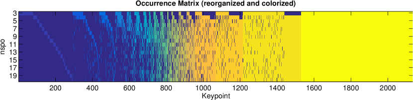
(d)

Figure 4: Influence of sampling density on keypoint stability. A set of increasingly dense and balanced scale-spaces is computed. The scale-space samplings are indexed by the ${n_{\text{spo}}}$ value, and ${\delta_{\text{min}}}$ is given by (23). (a) The number of detections is roughly constant for different sampling rates. (b) The rates of lost extrema (detected in the current sampling but not in the immediately finer sampling) and of new extrema (detected in the current sampling but not in the immediately coarser sampling) decrease with the sampling rate ${n_{\text{spo}}}$ and stabilize around $10\%$ of the total number of detections. (c) The occurrence matrix. Each row in this matrix corresponds to one of the simulated samplings (${n_{\text{spo}}}$), while each column indicates if a keypoint was detected in that particular sampling. (d) For better visualization, the columns are colored and reorganized in increasing order of stability (yellow: always detected, blue: detected only once). Almost $20\%$ of the detections appear for all scale-space sampling rates.

To illustrate how discrete extrema appear and disappear as scale-space sampling rates changes, we decided to investigate the stability of each single detected extremum. The set of all unique detected extrema was formed by gathering the extrema detected on all the simulated scale-spaces $\mathcal{D}_{\text{all}}=\cup_{i=1,\ldots,n}\mathcal{D}_{i}$ and then by extracting a unique set of detections $\mathcal{U}_{\text{all}}$. For each detected extremum $({\bf x},\sigma)\in\mathcal{U}_{\text{all}}$, we checked for its presence in each of the $\mathcal{D}_{i}$ detection sets. This was done by using the same definition as in (22). The results are summarized in the occurrence matrix shown in Figure 4 (c). Each simulated discretization is indexed by the ${n_{\text{spo}}}$ value. Each entry in this matrix indicates if a keypoint in $\mathcal{U}_{\text{all}}$ (column) was found in the scale-space with a given discretization $i=1,\ldots,n$ (where $i$ is the row index in the matrix).

We define the stability of a unique keypoint as the proportion of discretizations where it is detected. Figure 4 (d) shows the normalized occurence matrix, where each entry in the occurence matrix is multiplied by the stability value (therefore each column has the same color). Also, keypoints (columns) were reorganized from less to more stable (left to right).

The normalized occurrence matrix confirms that a majority of the keypoints are stable as they appear on at least 80% of the discretizations, and that some keypoints tend to appear and disappear repeatedly as sampling rates increase. It also shows that the proportion of unstable keypoints (e.g., those appearing less than 20% of the times) is low overall but is significantly larger for coarse discretizations than in denser ones.

5.3 Can unstable (intermittent) detections be detected?

To increase its overall detection stability, SIFT discards non-contrasted extrema based on their absolute DoG value. However, many other features, computed from the values of the extremum and its neighbors, could be used as well. The DoG value, the Laplacian of the DoG, the DoG Hessian condition number and the minimal absolute value of the difference between the extremum and its adjacent samples are some of them.

To find out if any of these simple features is good at predicting if a discrete extremum is stable (to different sampling rates), we proceeded as follows. Given the set of unique detections $\mathcal{U}_{\text{all}}$ computed by gathering all detections from the different scale-spaces with different sampling rates, we considered two subsets of unique keypoints: one subset of stable unique extrema (with occurrence rate above $80\%$) and one subset of unstable unique extrema (occurrence rate below $20\%$). Figure 5 (a–d) shows the proportion of extrema in both stable/unstable sets respectively, that have a feature value below a certain threshold. The considered features are: (a) the DoG value, (b) the Laplacian of the DoG, (c) the DoG Hessian condition number and (d) the minimal absolute value of the difference between the extremum and its adjacent samples.

This figure demonstrates that none of these features manages to faithfully separate the stable from the unstable ones. This is confirmed by the ROC curve shown in Figure 5 (e) (see figure caption for details). Noticeably, the keypoint feature giving the lowest discrimination performance is the DoG value used by SIFT.

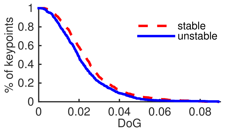
(a)

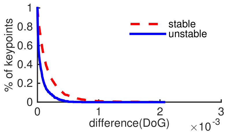
(b)

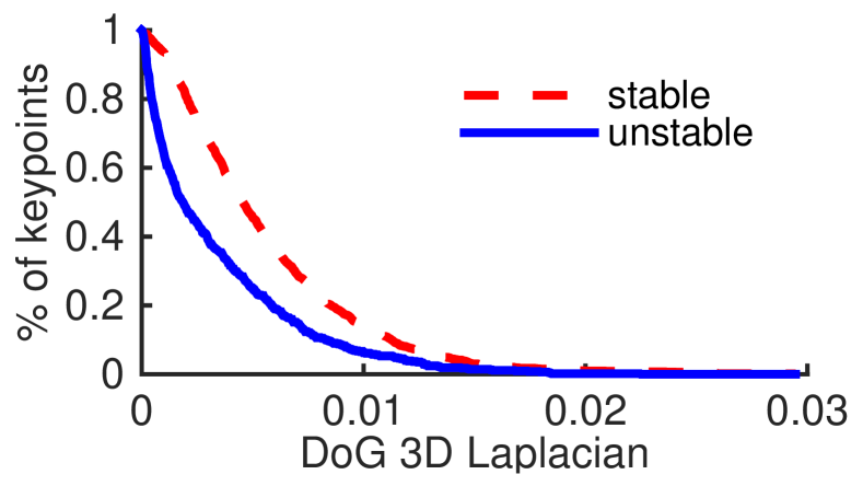
(c)

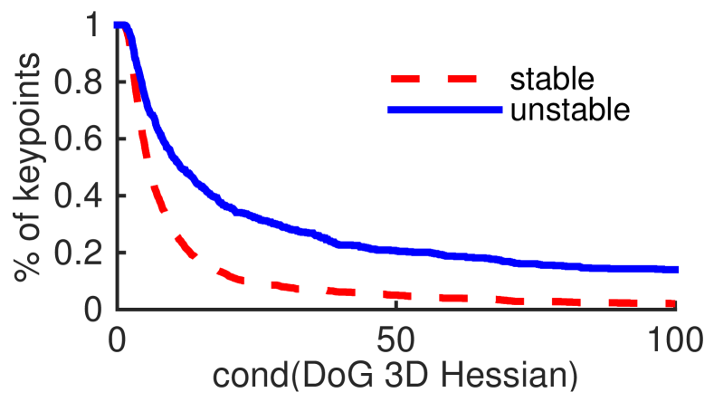
(d)

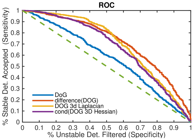
(e)

Figure 5: Attempts at filtering keypoints that are unstable to changes in the scale-space sampling. Increasing thresholds are applied respectively to the set of stable and unstable detections. The considered features are: (a) the extremum DoG value, (b) the difference of extremum DoG value and the adjacent samples in the scale-space, (c) the DoG 3d Laplacian value at the extremum, (d) the condition number of the DoG 3d Hessian at the extremum. None of the tested features separates convincingly the unstable from the stable detections. This is confirmed by the ROC curves, illustrating the performance of each feature, shown in (e). A point in a ROC curve indicates the proportion of non-filtered stable keypoints (good detections – sensitivity) as a function of the filtered unstable ones (good removals – specificity) for a particular threshold value. A perfect feature should produce a ROC that is always equal to $1$. According to this experiment, the worst feature for eliminating keypoints unstable to changes in the scale-space sampling is the DoG value.

5.4 Visualizing unstable (intermittent) detections

In an attempt to understand why the rudimentary detection and filtering procedures fail to avoid spurious detections, we examined visually some of the detected scale-space local structures. Figure 6 shows the DoG iso-surface computed around several stable and unstable keypoints from a very dense scale-space. Some detections are associated to isotropic shapes while others stem from elongated structures. There is no obvious link between how isotropic a structure is and its overall stability. As shown in the figure, some elongated structures produce stable detections. It seems therefore that a local analysis of the scale-space structure is not sufficient to characterize unstable detections.

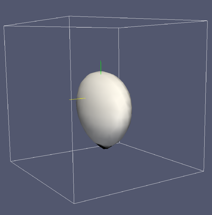
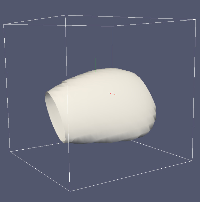
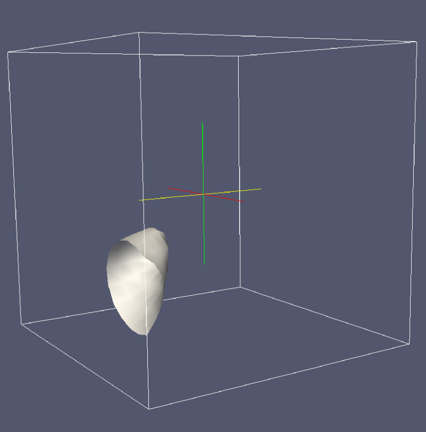
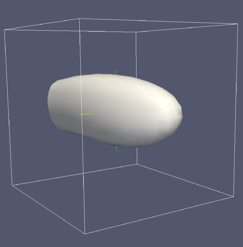
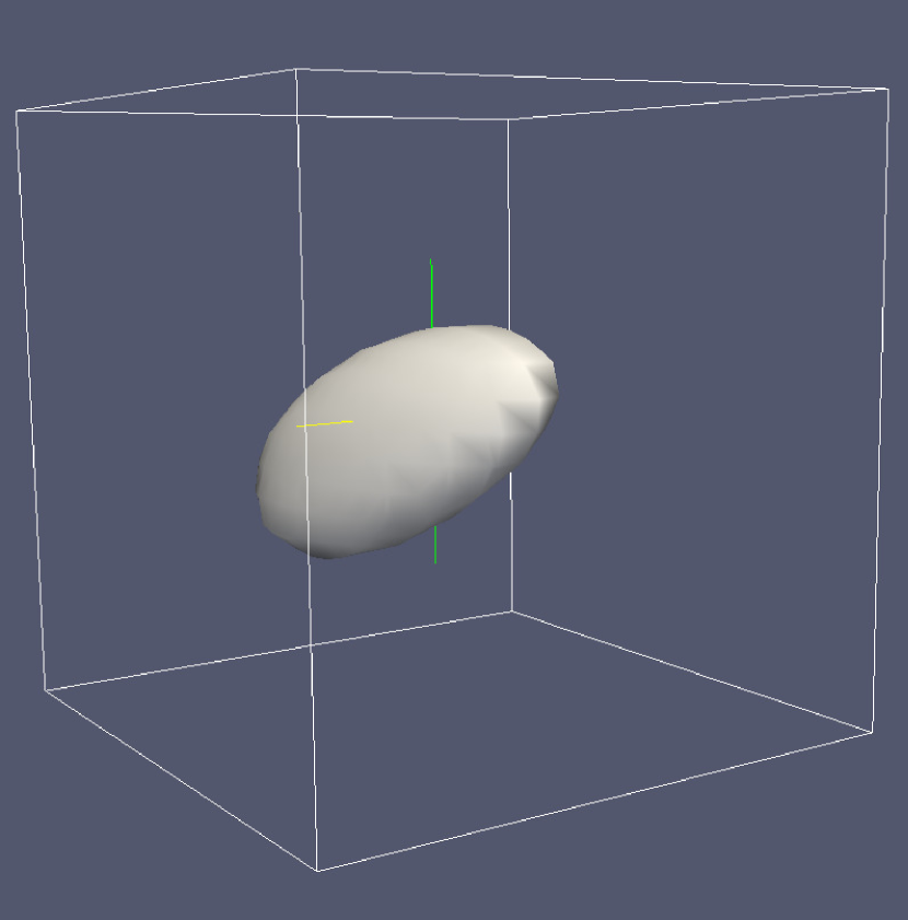
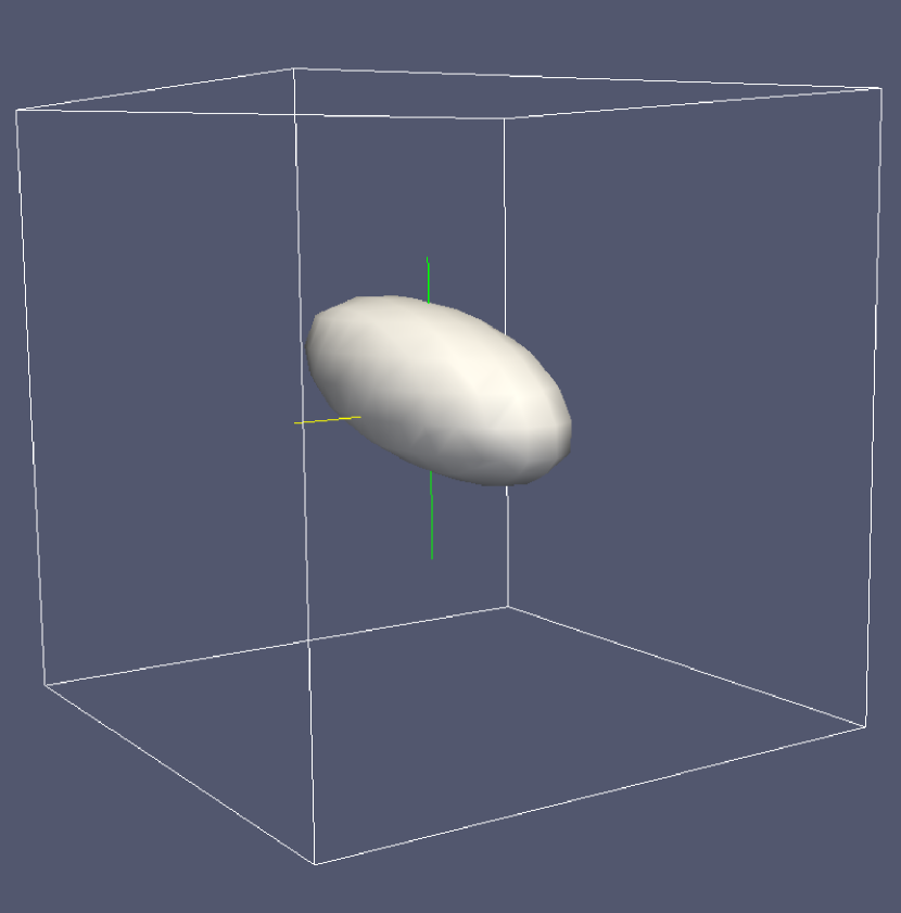
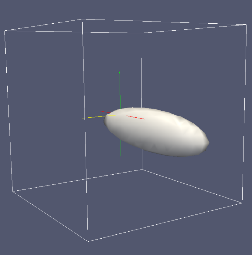
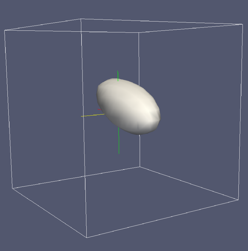
stable

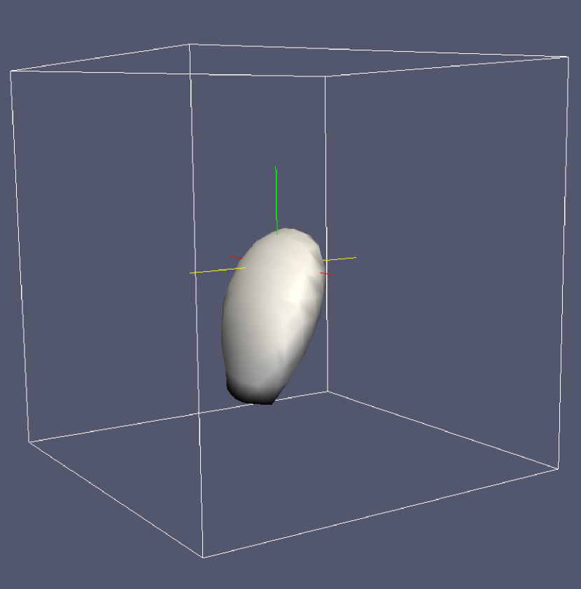
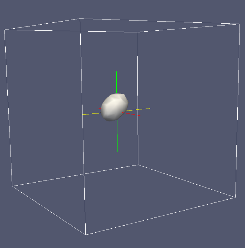
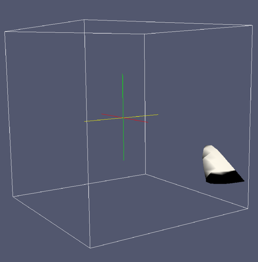
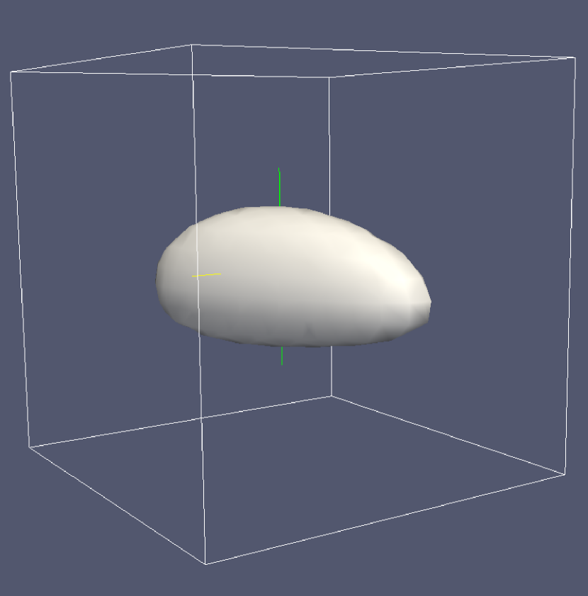
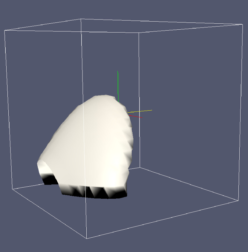
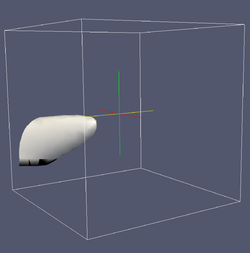
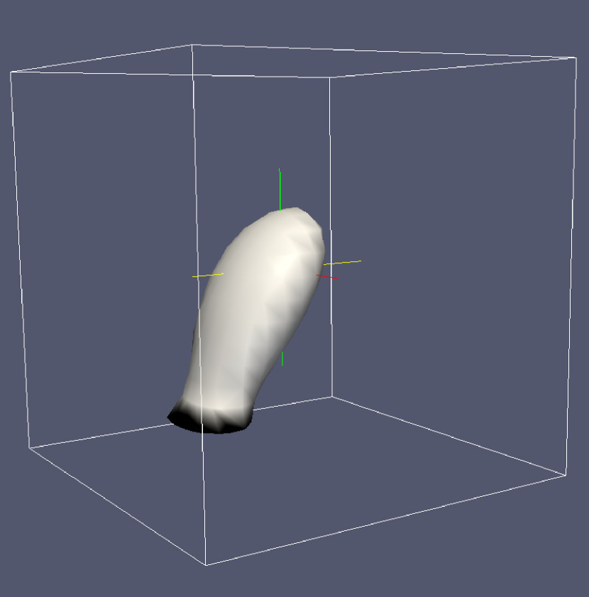
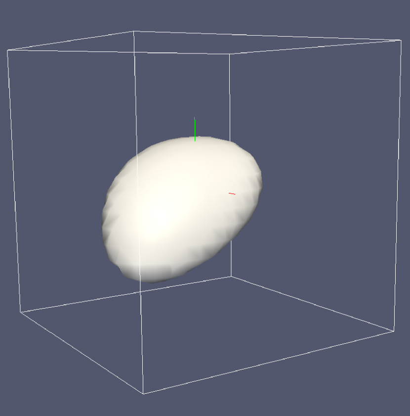
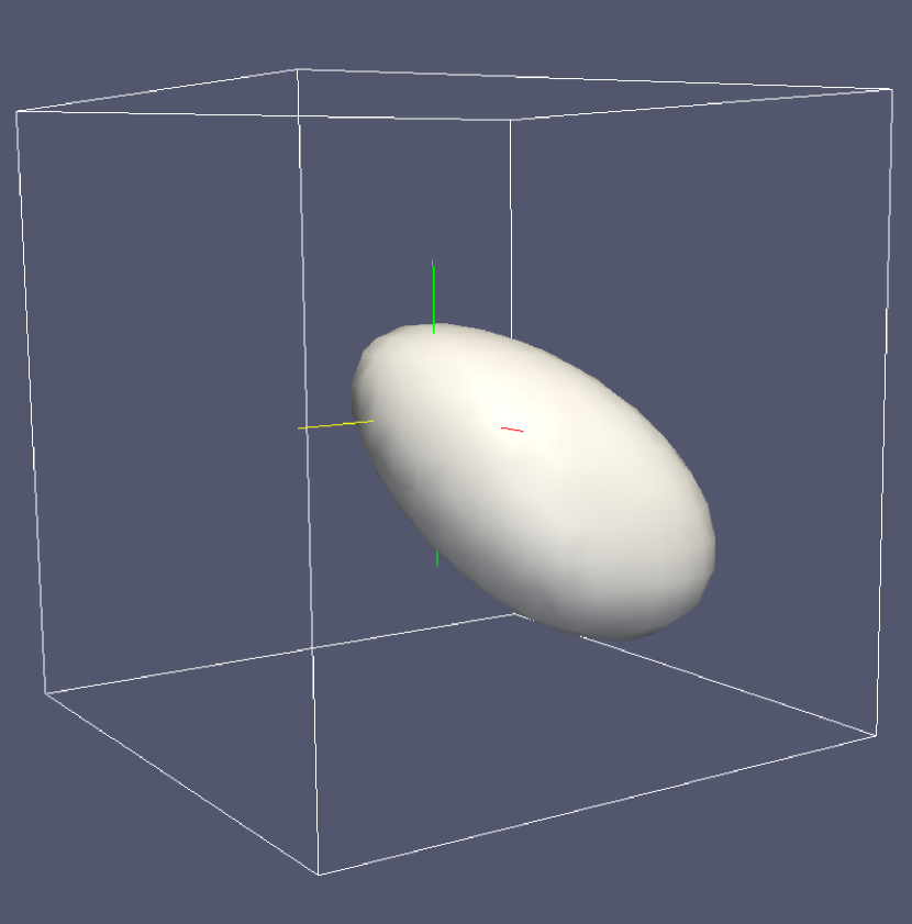
unstable

Figure 6: Illustration of the DoG scale-space around detected keypoints. DoG Iso-surfaces are computed from a dense scale-space. We observe a variety of configuration from isotropic shapes to elongated structures. Furthermore, there seems to be no obvious connection between the local structures and the keypoint’s stability level.

5.5 The influence of extrema interpolation on stability, precision and invariance

The refinement of the discrete extrema position proposed in SIFT has two main purposes. First, it allows to locate the extrema to subpixel accuracy thanks to a local continuous model of the DoG scale-space. But this refinement procedure also detects and discards unstable discrete extrema.

In this section, we analyze the impact of the refinement procedure. To that aim, we considered an input image and a series of transformations simulating small displacements of the camera. Although the analysis was restricted for a sake of simplicity to the case of translations and scale changes, it could be easily generalized to more complex image transformations such as perspective projections.

We examined the influence of the two main parameters in the refinement procedure (see Section 2.1): the maximal number of allowed interpolations $N_{\text{interp}}$, and the maximum offset $M_{\text{offset}}$ authorized for the extremum at each refinement iteration.

Our performance measure was the stability, measured by considering the number of keypoints that appear in at least a certain percentage of the simulated image transformations. A perfectly stable keypoint would be one that appears in all the simulated images, while a perfectly unstable keypoint would be one that only appears in one of the images. We also measured the precision by computing the average standard deviation of the location of the stable keypoints, where keypoints were considered stable if they appeared in at least $50\%$ of the simulated transformations.

Figure 7 (a,b) shows the percentage of unique keypoints that appear in at least a given percentage of the translations for different values of $M_{\text{offset}}$. Each figure corresponds to a given sampling rate (${n_{\text{spo}}}=3\text{ and }15$) and a given maximal number of interpolations ($N_{\text{interp}}=1,2,\infty$). Ideally, one would like to have a large proportion of stable detections, which would correspond to a flat curve. The percentage of detections for the SIFT sampling rate (${n_{\text{spo}}}=3$) decreases quickly when considering only the more stable ones, present in a large percentage of the simulated transformations. On the other hand, ${n_{\text{spo}}}=15$ leads to flatter curves, which implies more stable detections, and demonstrates that increasing the scale-space sampling improves stability. The refinement of the extrema helps discard the unstable ones.

The fact that the results with $N_{\text{interp}}=2$ and $N_{\text{interp}}=\infty$ are identical (second and third row of Figure 7), implies that there is no extra benefit in allowing more than two iterations. The present analysis indicates that allowing a maximum of two interpolations ($N_{\text{interp}}=2$) in combination with a maximum displacement of $M_{\text{offset}}=0.6$ produce on average keypoints that are more stable. This conclusion is independent of the considered ${n_{\text{spo}}}$. Therefore, for the remainder of the article, we consider the refinement step with these two values.

Increasing the scale-space sampling rate in conjunction with extrema interpolation has a tremendous impact on the detection precision. Figure 7 shows for both, discrete and interpolated detections, the mean of the precision of stable keypoints (appearing in at least $50\%$ of translations) as a function of the scale-space sampling rate.

We repeated the same experiment but different camera zoom-outs were simulated. The results are very similar to the pure camera translation case (see Figure 8). In general, sampling the scale-space finer than what is proposed in SIFT (e.g., ${n_{\text{spo}}}>3$) allows to better localize the DoG extrema. In addition, the local refinement of the extrema position increases the extrema precision. We repeated the experiments with different rotations and reached the same conclusions.

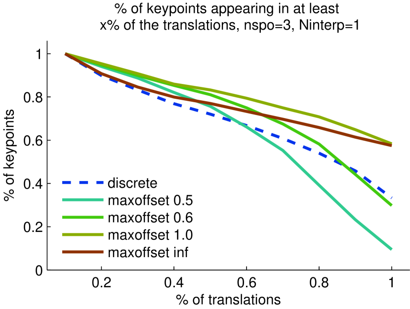
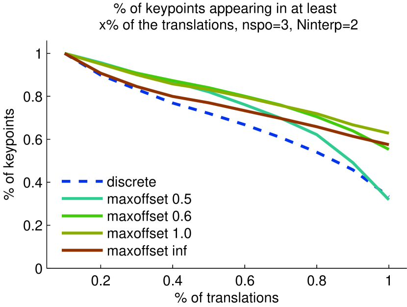
(a) ${n_{\text{spo}}}=3$

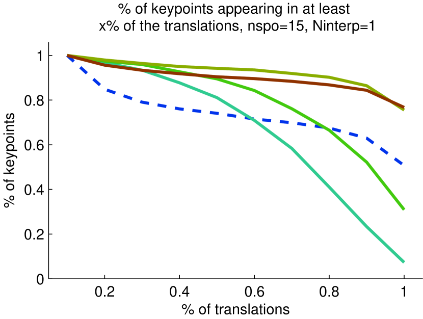
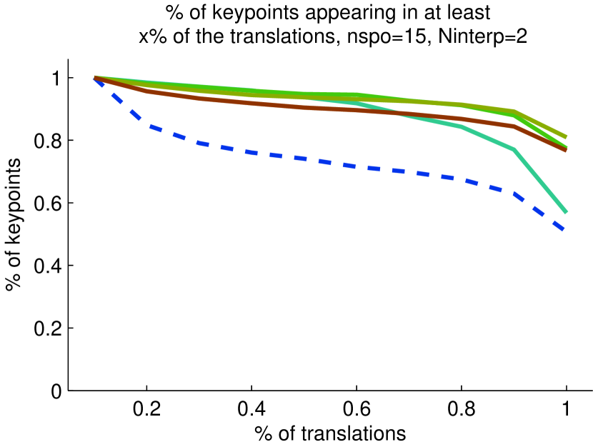
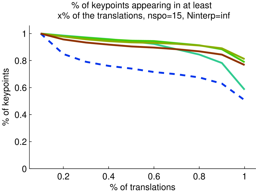
(b) ${n_{\text{spo}}}=15$

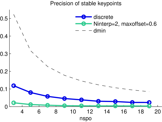
(c)

Figure 7: Influence of extrema refinement parameters $M_{\text{offset}}$ and $N_{\text{interp}}$ on the detection stability/precision. A set of translated images was simulated and the keypoints extracted. Each curve shows the percentage of unique keypoints appearing in at least a certain percentage of the simulated image translations for different values of $M_{\text{offset}}=0.5,0.6,1.0,\infty$. The plots in the first, second and third row were generated considering a maximum number of interpolations $N_{\text{interp}}=1,2\text{ and }\infty$ respectively. The left block of plots (a) was generated by sampling the scale-space with ${n_{\text{spo}}}=3$ (and the corresponding ${\delta_{\text{min}}}$), while the right block (b) was generated using ${n_{\text{spo}}}=15$. Allowing two iterations ($N_{\text{interp}}=2$) and a maximal offset of $M_{\text{offset}}=0.6$ gives the best performance in terms of stability of detected keypoints. Allowing for more interpolations attempts did not increase the performance, as can be seen by comparing the third row to the second row. (c) shows the influence of the extrema refinement on the precision of the stable set of keypoints (appearing in at least $50\%$ of the simulated images). In this pure translation scenario, it appears that the precision of the detected extrema significantly increases when using extrema interpolation and when sampling finely the scale-space (e.g., ${n_{\text{spo}}}>3$).

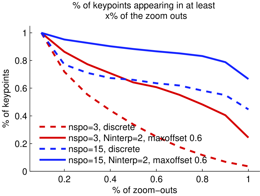
(a)

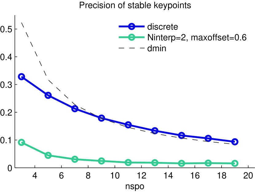
(b)

Figure 8: Influence of scale-space sampling and extrema refinement on the invariance to zoom-outs. A set of zoomed-out images was simulated, scale-space were computed and the keypoints extracted and those which were detected outside the commonly covered scale range were discarded. (a) The percentage of unique detections appearing in at least a certain percentage of the simulated images for different scale-space sampling and refinements. The best performance is obtained by significantly oversampling the scale-space, with ${n_{\text{spo}}}=15$, and by refining the extrema with the local interpolation. In this case, most of the detected keypoints are present in all the simulated images. On the other hand, the original SIFT sampling ${n_{\text{spo}}}=3$ leads to low stability even with the extrema refinement step. (b) Mean precision of stable keypoints location (appearing in at least $50\%$ of the zoom-outs) plotted as a function of the sampling rate ${n_{\text{spo}}}$. The local refinement of the extrema position significantly increases the precision of the extrema detection. Also, using a finer grid than the one proposed in SIFT (e.g., ${n_{\text{spo}}}>3$) allows to better localize the extrema.

5.6 Influence of $\kappa$

The DoG scale-space is formed by computing the difference of Gaussians operator at scales $\kappa\sigma$ and $\sigma$. To analyze the influence of the DoG parameter $\kappa$, we computed the extrema of different DoG scale-spaces produced with $\kappa=2^{\nicefrac{{1}}{{30}}},2^{\nicefrac{{1}}{{29}}},\ldots,2^{\nicefrac{{1}}{{2}}}$. In order to minimize sampling related instability, the scale-spaces were sampled at ${n_{\text{spo}}}=15$ and the respective ${\delta_{\text{min}}}$.

The number of detected extrema is more or less constant for different values of $\kappa$ (Figure 9 (a)) Depending on the $\kappa$ value, the same structure is detected at a different scale. As pointed out in Section 2.3, a Gaussian blob of standard deviation $\sigma$ produces an extrema of the DoG at scale $\sigma/\sqrt{\kappa}$. Thus, we have normalized the detections scale by $\sigma_{\text{normalized}}=\sigma\sqrt{\kappa}$. To compare the keypoints detected with different $\kappa$ values, we also restricted the analysis to those lying on the common scale range, that is, ${\sigma_{\text{min}}}\sqrt{2^{1/2}}\leq\sigma\leq 2{\sigma_{\text{min}}}\sqrt{2^{1/30}}.$

We proceeded similarly as before by gathering all the detections from the different DoG scale-spaces and computed a set of unique detections. Then, we proceeded to create the occurrence matrix. The occurrence matrix in Figure 9 (b) shows that the different $\kappa$’s lead for the most part to identical detections. Almost half the keypoints are detected in every DoG scale-space and a large percentage of the keypoints is detected in most simulated scale-spaces.

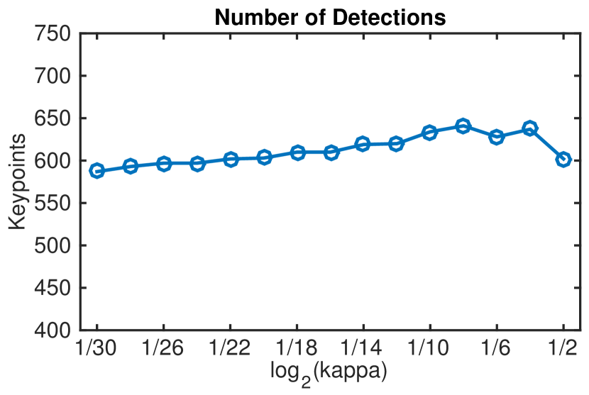
(a)

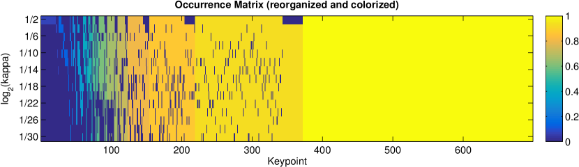
(b)

Figure 9: Influence of the DoG parameter $\kappa$. The number of detected keypoints is roughly constant for different values of $\kappa$ (a) . The occurrence matrix for the set of unique normalized keypoints detected in the different DoG scale-spaces (b). A large majority of the keypoints are detected in most simulated scale-spaces when changing the value of $\kappa$.

6 Impact of deviations from the perfect camera model

In order to achieve perfect invariance, SIFT formally requires that the image is acquired in perfect conditions. This means that the input image should be noiseless, well-sampled (according to the Nyquist-Shannon sampling theorem) and with an a priori known level of Gaussian blur $c$. These ideal conditions justify the construction of the image scale-space. In this section, we evaluate what happens when there are deviations from these ideal requirements.

6.1 Image aliasing

Let us assume that the input image was generated with a camera having a Gaussian point-spread-function of standard deviation $c$. If $c$ is low (i.e., $c\leq 0.7$) the acquired image will be subject to aliasing artifacts. We shall assume first that this camera blur $c$ is known beforehand, so that the SIFT method can be applied consistently.

To evaluate the SIFT performance in this aliasing situation, we simulated random translations of the digital camera. Then, we computed the extrema of the DoG scale-spaces generated with each translated image and compared the extrema. All scale-space consisted of one octave computed with ${n_{\text{spo}}}=15$, ${\sigma_{\text{min}}}=1.1$ and the interpolation parameters were set to $N_{\text{interp}}=2$ and $M_{\text{offset}}=0.6$.

Figure 10 (a) shows the average number of keypoints detected as a function of the camera blur $c$. The number of detections is independent of the camera blur. Indeed, a sharper shot does not increase the number of keypoints.

In Figure 10 (b) we show the percentage of unique keypoints that appear in at least a certain percentage of the translated images. Keypoints detected from well sampled images (e.g., $c>0.6$) are stable to translation (the curves are almost flat) while those from severely undersampled images ($c\approx 0.3$) are very sensitive to the position of the sampling grid, as expected.

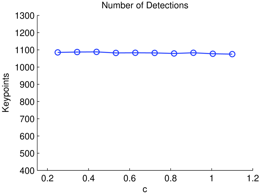
(a)

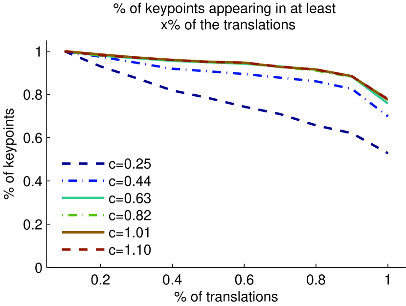
(b)

Figure 10: Impact of image aliasing. For various camera blurs, $0.25\leq c\leq 1.1$, a set of translated images were simulated and the DoG keypoints extracted (${n_{\text{spo}}}=15$, ${\sigma_{\text{min}}}=1.1$). Aliasing does not affect the number of detections (a). In (b) we show the percentage of unique keypoints appearing in at least a certain percentage of the simulated translations. Detections are less stable for severely aliased images ($c=0.25$), while for $c>0.6$, the impact of aliasing is negligible.

6.2 Unknown input image blur level

A more realistic scenario is the case where the level of blur of the input image $c$ is unknown. SIFT requires this value to create the scale-space starting at a known level of image blur ${\sigma_{\text{min}}}$. A wrong assumption of the input camera blur affects the range of simulated scales simulated in the Gaussian scale-space.

To demonstrate to what extent the wrong knowledge of the input camera blur produces unrelated keypoints, we compared the keypoints extracted assuming an image blur of $c=0.7$ from a set of images having actual random blur $c_{\text{real}}$ uniformly picked from $[c-\Delta c,c+\Delta c]$.

Figure 11 shows the number of unique keypoints that appear in at least a certain percentage of the simulated images. This was evaluated for different ranges of uncertainty (i.e., $\Delta c=0.05-0.4$). The larger the range of uncertainty $\Delta c$, the more unrelated the extrema are (the curve decreases very fast, indicating the presence of many unique keypoints appearing in only a few of the simulated images). Figure 11(b) explores the influence of detection scale on stability to wrong blur assumption. The percentage of unique keypoints appearing in at least 70% of the simulated images is shown as a function of scale. The influence of a wrong assumption decreases with detection scales.

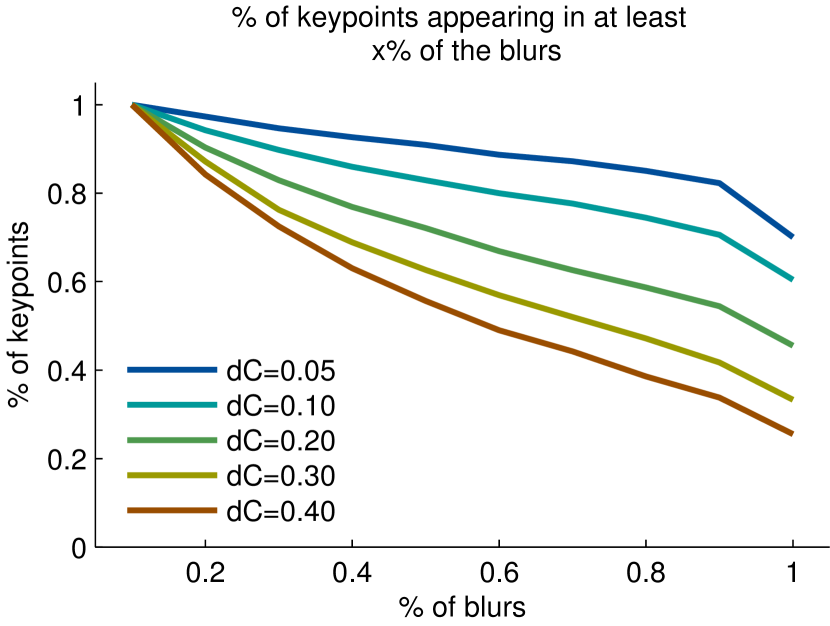
(a)

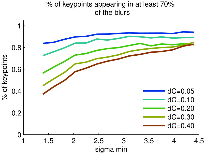
(b)

Figure 11: The impact of a wrong assumption on the camera blur. Comparison of the keypoints extracted assuming $c=0.7$ when the real camera blur was picked randomly in $[c-\Delta c,c+\Delta c]$. (a) The percentage of unique keypoints that appear in at least a certain percentage of the simulated images is plotted for different levels of uncertainty on camera blur ($\Delta c=0.05-0.4$). (b) Influence of scale on stability to wrong blur assumption. For keypoints detected at scales ranging from $\sigma_{\text{min}}$ and $2\sigma_{\text{min}}$, the proportion of unique keypoints that appear in at least 70% of the simulated images is shown as a function of scale $\sigma_{\text{min}}$. The impact of a wrong blur level assumption decreases as we consider detections at larger scale (i.e., large $\sigma_{\text{min}}$).

6.3 Image noise

The digital image acquisition is always affected by noise that undermines the performance of SIFT. To evaluate the impact of image noise we simulated different image acquisition, by adding random white Gaussian noise to the input image. Then, we proceeded to compute the keypoints that are detected in a certain percentage of the simulated images.

Figure 12 shows results when considering set of input images with increasing level of noise.

Specifically, Figure 12 (a) shows the percentage of unique keypoints that appear in at least a certain percentage of the simulated images.

It demonstrates the strong impact of noise level on keypoint stability. Such impact however is mitigated for detections at larger scales. In a Gaussian scale-space, the level of noise decreases as the scale increases. In fact, the noise standard deviation observed in a given octave is half the one observed in the previous octave. This is confirmed in Figure 12 (d), which shows, for keypoints detected in a range of scale $[\sigma_{\text{min}},2\sigma_{\text{min}}]$, the proportion of unique keypoints that appear in at least 70% of the simulated noisy image as a function of scale $\sigma_{\text{min}}$.

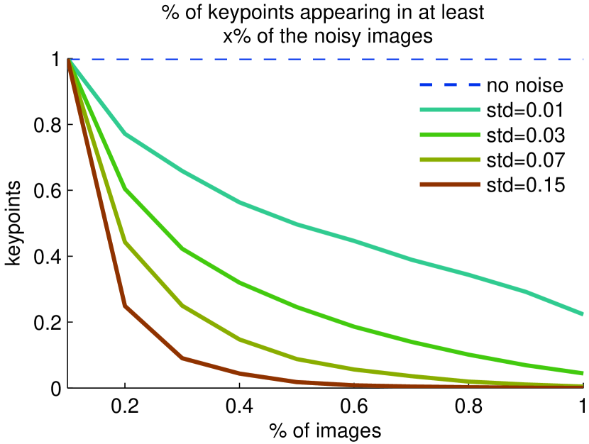
(a)

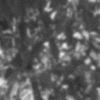
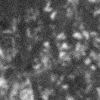
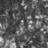
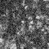
(b)

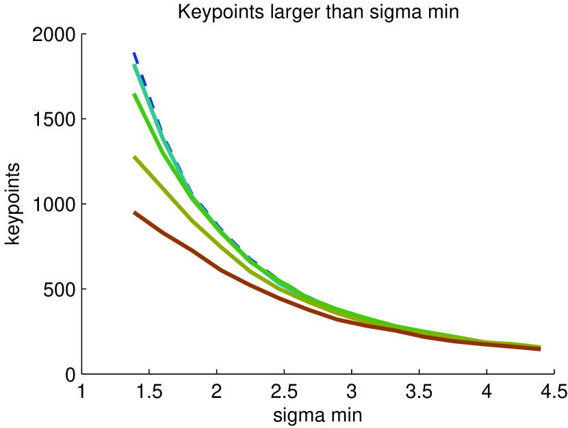
(c)

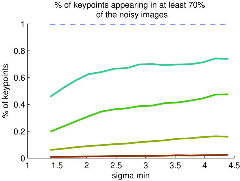
(d)

Figure 12: Impact of image noise. (a) The proportion of unique keypoints that appear in at least a certain proportion of the simulated images is plotted for different levels of image noise. Noise has a significant impact on the DoG extrema detection. (b) Crops of the input images simulated with $c=0.8$ and added Gaussian white noise of standard deviation $\sigma_{\text{noise}}=0.01,0.03,0.07\text{ and }0.15$. (c) Number of keypoints detected at a scale larger than ${\sigma_{\text{min}}}$ as a function of ${\sigma_{\text{min}}}$. The number of detections decreases as the level of noise increases. (d) Influence of scale on stability to noise. For keypoints detected at scales ranging from $\sigma_{\text{min}}$ to $2\sigma_{\text{min}}$, the proportion of unique keypoints that appear in at least 70% of the simulated images is shown a function of scale $\sigma_{\text{min}}$. Unsurprisingly we observe that, for a given level of noise, the stability in the second octave is comparable to the stability achieved in the first octave with half the level of noise.

7 Concluding remarks

We presented a systematic analysis of the main steps involved in the detection of keypoints in the SIFT algorithm. One of the main conclusions is that the original parameter choice in SIFT is not sufficient to ensure a theoretical and practical scale (and even translation) invariance, which was the main claim of the SIFT method. In addition, we showed that the SIFT invariance claim is strongly affected if the assumption on the level of blur in the input image is wrong.

Specifically, we showed that increasing the scale-space sampling from ${n_{\text{spo}}}=3$ to ${n_{\text{spo}}}=15$ (and respectively the space sampling rate ${\delta_{\text{min}}}$) improves the stability of the detected keypoints. This implies that if a series of image transformations (e.g., translations, zoom-outs) are applied to an image, the keypoints detected in one of them will be detected with high probability in all the others. This stability property is fundamental for fulfilling the scale invariance claim. The extrema refinement was shown to improve both the precision and the stability of the detected keypoints. We showed that the largest number of stable keypoints is achieved with parameters $M_{\text{offset}}=0.6$ and $N_{\text{interp}}=2$ (while SIFT recommends $N_{\text{interp}}=5$). We also demonstrated that the DoG threshold fails to filter out unstable keypoints, and that the different definitions of the DoG scale-space (parameter $\kappa$) lead for the most part to identical detections up to a normalization of the scale. Finally, we showed how the presence of aliasing and noise in the acquired image deteriorate detections stability.

References

- [1] D. Lowe, “Object recognition from local scale-invariant features,” in ICCV, 1999.
- [2] ——, “Distinctive image features from scale-invariant keypoints,” IJCV, vol. 60, pp. 91–110, 2004.
- [3] M. Brown and D. Lowe, “Automatic panoramic image stitching using invariant features,” IJCV, vol. 74, no. 1, pp. 59–73, 2007.
- [4] F. Riggi, M. Toews, and T. Arbel, “Fundamental matrix estimation via TIP-transfer of invariant parameters,” in ICPR, 2006.
- [5] C. Strecha, W. von Hansen, L. Van Gool, P. Fua, and U. Thoennessen, “On benchmarking camera calibration and multi-view stereo for high resolution imagery,” in CVPR, 2008.
- [6] J.-M. Morel and G. Yu, “Is SIFT scale invariant?” Inverse Problems and Imaging, vol. 5, no. 1, pp. 115–136, 2011.
- [7] J. Weickert, S. Ishikawa, and A. Imiya, “Linear scale-space has first been proposed in Japan,” J. Math. Imaging Vision, vol. 10, no. 3, pp. 237–252, 1999.
- [8] T. Lindeberg, Scale-space theory in computer vision. Springer, 1993.
- [9] T. Tuytelaars and K. Mikolajczyk, “Local invariant feature detectors: A survey,” Found. Trends in Comp. Graphics and Vision, vol. 3, no. 3, pp. 177–280, 2008.
- [10] H. Bay, T. Tuytelaars, and L. van Gool, “SURF: Speeded Up Robust Features,” in ECCV, 2006.
- [11] K. Mikolajczyk, T. Tuytelaars, C. Schmid, A. Zisserman, J. Matas, F. Schaffalitzky, T. Kadir, and L. Van Gool, “A comparison of affine region detectors,” IJCV, vol. 65, no. 1-2, pp. 43–72, 2005.
- [12] W. Förstner, T. Dickscheid, and F. Schindler, “Detecting interpretable and accurate scale-invariant keypoints,” in ICCV, 2009.
- [13] P. Mainali, G. Lafruit, Q. Yang, B. Geelen, L. Van Gool, and R. Lauwereins, “SIFER: Scale-Invariant Feature Detector with Error Resilience,” IJCV, vol. 104, no. 2, pp. 172–197, 2013.
- [14] C. Ancuti and P. Bekaert, “SIFT-CCH: Increasing the SIFT distinctness by color co-occurrence histograms,” in ISPA. IEEE, 2007, pp. 130–135.
- [15] O. Pele and M. Werman, “A linear time histogram metric for improved SIFT matching,” in ECCV. Springer, 2008, pp. 495–508.
- [16] J. Rabin, J. Delon, and Y. Gousseau, “A statistical approach to the matching of local features,” SIAM J. Imaging Sci., vol. 2, no. 3, pp. 931–958, 2009.
- [17] Y. Ke and R. Sukthankar, “PCA-SIFT: A more distinctive representation for local image descriptors,” in CVPR, 2004.
- [18] M. Calonder, V. Lepetit, C. Strecha, and P. Fua, “BRIEF: Binary Robust Independent Elementary Features,” in ECCV. Springer, 2010, pp. 778–792.
- [19] E. Rublee, V. Rabaud, K. Konolige, and G. Bradski, “ORB: An efficient alternative to SIFT or SURF,” in ICCV, 2011.
- [20] E. Tola, V. Lepetit, and P. Fua, “A fast local descriptor for dense matching,” in CVPR, 2008.
- [21] ——, “DAISY: An efficient dense descriptor applied to wide-baseline stereo,” PAMI, vol. 32, no. 5, pp. 815–830, 2010.
- [22] A. Vedaldi and B. Fulkerson, “VLFeat: An open and portable library of computer vision algorithms,” in Proc. ACM Int. Conf. Multimed., 2010.
- [23] S. Leutenegger, M. Chli, and R. Siegwart, “BRISK: Binary Robust Invariant Scalable Keypoints,” in ICCV, 2011.
- [24] M. Agrawal, K. Konolige, and M. Blas, “CenSurE: Center Surround Extremas for Realtime Feature Detection and Matching,” in ECCV. Springer, 2008, pp. 102–115.
- [25] S. Winder and M. Brown, “Learning local image descriptors,” in CVPR, 2007.
- [26] S. Winder, G. Hua, and M. Brown, “Picking the best DAISY,” in CVPR, 2009.
- [27] J. Chen, S. Shan, C. He, G. Zhao, M. Pietikainen, X. Chen, and W. Gao, “WLD: A robust local image descriptor,” PAMI, vol. 32, no. 9, pp. 1705–1720, 2010.
- [28] M. Grabner, H. Grabner, and H. Bischof, “Fast approximated SIFT,” in ACCV. Springer, 2006, pp. 918–927.
- [29] C. Liu, J. Yuen, A. Torralba, J. Sivic, and W. Freeman, “SIFT Flow: Dense correspondence across different scenes,” in ECCV. Springer, 2008, pp. 28–42.
- [30] P. Moreno, A. Bernardino, and J. Santos-Victor, “Improving the SIFT descriptor with smooth derivative filters,” Pattern Recognition Lett., vol. 30, no. 1, pp. 18–26, 2009.
- [31] M. Brown, R. Szeliski, and S. Winder, “Multi-image matching using multi-scale oriented patches,” in CVPR, 2005.
- [32] T. Dickscheid, F. Schindler, and W. Förstner, “Coding images with local features,” IJCV, vol. 94, no. 2, pp. 154–174, 2011.
- [33] R. Sadek, C. Constantinopoulos, E. Meinhardt, C. Ballester, and V. Caselles, “On affine invariant descriptors related to SIFT,” SIAM, vol. 5, no. 2, pp. 652–687, 2012.
- [34] I. Rey-Otero, J.-M. Morel, and M. Delbracio, “An analysis of scale-space sampling in SIFT,” in Image Processing (ICIP), 2014 IEEE International Conference on. IEEE, 2014, pp. 4847–4851.
- [35] K. Mikolajczyk and C. Schmid, “A performance evaluation of local descriptors,” PAMI, vol. 27, no. 10, pp. 1615–1630, 2005.
- [36] K. Van De Sande, T. Gevers, and C. Snoek, “Evaluating color descriptors for object and scene recognition,” PAMI, vol. 32, no. 9, pp. 1582–1596, 2010.
- [37] I. Rey-Otero and M. Delbracio, “Anatomy of the SIFT Method,” Image Processing On Line, vol. 4, pp. 370–396, 2014.
- [38] ——, “Computing an Exact Gaussian Scale-space,” 2014, preprint.
- [39] R. Sadek, “Some problems on temporally consistent video editing and object recognition,” Ph.D. dissertation, Universitat Pompeu Fabra, 2012.
- [40] M. Delbracio, P. Musé, and A. Almansa, “Non-parametric sub-pixel local point spread function estimation,” IPOL, 2012.