Theoretical Prediction of the Nematic Orbital-Ordered State
in Ti-Oxypnictide Superconductor BaTi₂(As,Sb)₂O

Abstract

The electronic nematic state without magnetization emerges in various strongly correlated metals such as Fe-based and cuprate superconductors. To understand this universal phenomenon, we focus on the nematic state in Ti-oxypnictide BaTi₂(As,Sb)₂O, which is expressed as the three-dimensional 10-orbital Hubbard model. The antiferromagnetic fluctuations are caused by the Fermi surface nesting. Interestingly, we find the spin-fluctuation-driven orbital order due to the strong orbital-spin interference, which is described by the Aslamazov-Larkin vertex correction (AL-VC). The predicted intra-unit-cell nematic orbital order is consistent with the recent experimental reports on BaTi₂(As,Sb)₂O. Thus, the spin-fluctuation-driven orbital order due to the AL-VC mechanism is expected to be universal in various two- and three-dimensional multiorbital metals.

I Introduction

Various interesting symmetry breaking phenomena associated with the charge, orbital, and spin degrees of freedom emerge in strongly correlated electron systems. Among them, the rotational symmetry breaking, so called the nematic transition, has attracted increasing attention, after the discovery of the nematic order in Fe-based and cuprate superconductors. In Fe-based superconductors, both the spin-nematic order Fernandes ; DHLee ; Chubukov ; QSi and the orbital order Kruger ; PP ; WKu ; Onari-SCVC ; Onari-SCVCS ; Text-SCVC ; JP are considered as the origin of the nematic order. In cuprates, the $p$-orbital order is a promising candidate for the nematic Yamakawa-CDW ; Tsuchiizu-CDW , whereas other promising scenarios had been proposed so far DHLee-cup ; Kivelson-cup ; Chubukov-cup ; Sachdev-cup . The nematic transitions in these superconductors cannot be understood within the random-phase-approximation (RPA) based on the Hubbard models, so it is demanded to develop the microscopic theory beyond the mean-field-level approximations.

To achieve the fundamental understanding of the electronic nematic states, we focus on the nematic phase in the Ti-oxypnictide superconductors YajimaJPSJ2012 ; YajimaJPSJ2013 ; Zhai2013 ; Wang2010 . No magnetic order appears in the nematic phase NMR ; Rohr , similarly to FeSe. The nematic order in Ti-oxypnictides is driven by the electron-interaction since the orthorhombic lattice deformation $(a-b)/(a+b)$ is just $\sim 0.1$% Frandsen2014 , which is even smaller than that in Fe-based superconductors. In contrast to these systems, the lattice distortions in Jahn-Teller systems (like Mn-oxides) reach a few %. The nematic order in BaTi₂As₂O is ascribed to the intra-unit-cell charge-density-wave (CDW) with $d$-wave symmetry since no superlattice was found by the electron diffraction studies Frandsen2014 ; Nozaki . This result is analogous to the “$d$-symmetry CDW” in under-doped cuprates in Refs. Yamakawa-CDW ; Tsuchiizu-CDW ; STM-Fujita-cup . Such intra-unit-cell CDW in Ti-oxypnictide is unable to be explained by the electron-phonon mechanism Subedi . Thus, the study of Ti-oxypnictides should serve to understand the origin of the nematicity due to the electron-interaction.

Interestingly, the superconducting phase (with $T_{\rm c}\sim 5$K) is realized near the nematic phase in various Ti-oxypnictides, indicating the importance of the nematic fluctuations on the superconductivity. In addition, strong antiferromagnetic (AFM) spin fluctuations appear near the nematic phase in BaTi₂Sb₂O NMR , analogously to the Fe-based and cuprate superconductors. Therefore, Ti-oxypnictides would give us great hints to understand the close interplay between the nematicity, magnetism, and superconductivity, which is a central issue in Fe-based and cuprate superconductors.

In this paper, we study the origin of the non-magnetic nematic order in Ti-oxypnictides based on the realistic Hubbard model for BaTi₂(As,Sb)₂O. Due to the Fermi surface (FS) nesting, the AFM fluctuations develop at ${{\bm{Q}}}_{s}=(\pi,0,\pi)$ and $(0,\pi,\pi)$, consistently with the previous theoretical studies Yu ; Singh and the NMR study NMR . Remarkably, we find that the strong orbital fluctuations at ${{\bm{q}}}=(0,0,0)$ are induced by the Aslamazov-Larkin vertex correction (AL-VC), which is neglected in the RPA. We predict the formation of the spin-fluctuation-driven intra-unit-cell orbital order in BaTi₂(As,Sb)₂O. Thus, the nematic orbital order due to the AL-VC is realized in Ti-oxypnictides, similarly to Fe-based and cuprate superconductors.

The AL-VC represents the orbital-spin interplay, which is intuitively understood in terms of the strong-coupling picture $U\gg W_{\rm band}$ as we explained in Ref. Onari-SCVCS : In Fe-based superconductors, the ferro-orbital order $n_{xz}\gg n_{yz}$ gives rise to the strong anisotropy in the nearest-neighbor exchange interaction, $J^{(1)}_{x}\neq J^{(1)}_{y}$, and therefore the stripe AFM order with is induced. Thus, the orbital-order/fluctuations and magnetic-order/fluctuations simultaneously emerges. Such Kugel-Khomskii-type orbital-spin interplay is explained by the AL-VC in the weak-coupling picture.

II Model Hamiltonians

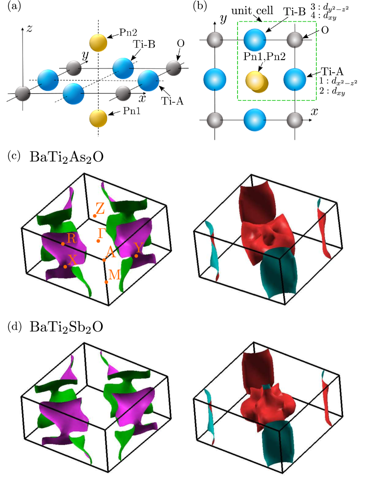
Figure 1: (a) Crystal structure of Ti₂Pn₂O-layer and (b) unit cell with two Ti-ions and two Pn-ions. (c) Three-dimensional FSs for BaTi₂As₂O and (d) FSs for BaTi₂Sb₂O obtained by the band calculation.

Figures 1 (a) and (b) show the metallic Ti₂Pn₂O-layer in Ti-oxypnictides (Pn=As, Sb). The unit cell contains two Ti-sites and two Pn-sites. The bandstructure near the Fermi level is mainly composed of ($d_{x^{2}-z^{2}}$, $d_{xy}$)-orbitals on Ti-A and ($d_{y^{2}-z^{2}}$, $d_{xy}$)-orbitals on Ti-B, which are respectively denoted as (1, 2) and (3, 4) hereafter. Here, we perform the band calculation of BaTi₂Pn₂O using the WIEN2K software, In Fig. 1, we show the FSs for (c) BaTi₂As₂O and the FSs for (d) BaTi₂Sb₂O given by the WIEN2K software. The crystal structures are respectively given in Ref. Wang2010 and Ref. YajimaJPSJ2012 . In both compounds, the FSs are composed by the hole-like cylinder FSs around X and Y points, the electron-like cylinder FS around M point, and three-dimensional FSs around $\Gamma$ point. The shape of the three cylinder FSs are very similar in both compounds. Although the shape of the three-dimensional FSs is different between these compounds, these FSs play a minor role on the orbital fluctuation mechanism.

Next, we derive three-dimensional 10-orbital tight-binding model for BaTi₂Pn₂O, with the four $d$-orbitals (orbital $1\sim 4$) and six $p$-orbitals of Pn1,2 (orbital $5\sim 10$), using the WANNIER90 software. The tight-binding hopping parameters for BaTi₂(As_1-xSb_x)₂O is approximately given by the interpolation between the parameters for BaTi₂As₂O and the parameters for BaTi₂Sb₂O. In this paper, we present the numerical study for BaTi₂(As_0.5Sb_0.5)₂O: We verified that the numerical results are essentially unchanged by $x$. The electron number per unit cell (two Ti ions and two Pn ions) is $14.0$. The bandstructure and the FSs in the $k_{z}=0$, $k_{z}=\pi/2$, and $k_{z}=\pi$ planes are shown in Figs. 2 (a)-(c), respectively. The red (blue) lines represents the electron-like (hole-like) FSs. The two hole-like cylinder FSs around X,Y points and the one electron-like cylinder FS around M point give the dominant density-of-states (DOS) at the Fermi level. The nesting between these FSs gives the spin fluctuations at $Q_{s}=(\pi,0,\pi)$ and $(0,\pi,\pi)$. In addition, complex three-dimensional FSs exist around $\Gamma$ point.

Figure 2: (color online) (a)-(c) Bandstructure and FSs in the $k_{z}=0$, $k_{z}=\pi/2$, and $k_{z}=\pi$ planes. The red and blue lines correspond to electron-like FSs and hole-like FSs, respectively.

The multiorbital Coulomb interaction term is given as

$$\!\!\!\!\!\!\!\!\!\!H_{\rm M}^{U}=\frac{1}{2}\sum_{i,l,{\sigma}\neq{\sigma}^{\prime}}Un_{i,l{\sigma}}n_{i,l,{\sigma}^{\prime}}+\frac{1}{2}\sum_{i,l\neq m,{\sigma},{\sigma}^{\prime}}\left\{U^{\prime}n_{i,l{\sigma}}n_{i,m,{\sigma}^{\prime}}\right.$$

$$\left.+J_{m,l}c_{i,m{\sigma}}^{\dagger}c_{i,l{\sigma}}(c_{i,l{\sigma}^{\prime}}^{\dagger}c_{i,m{\sigma}^{\prime}}+c_{i,m{\sigma}^{\prime}}^{\dagger}c_{i,l{\sigma}^{\prime}}\delta_{{\sigma},-{\sigma}^{\prime}})\right\},$$ (1)

where $U$ and $U^{\prime}$ are the intra-orbital and inter-orbital Coulomb interactions, and $J$ is the Hund’s interactions for $d$-electrons. Hereafter, we assume the relation $U=U^{\prime}+2J$ and $J>0$, and fix the ratio $J/U=1/9$ except in Fig. 5 (d): We verified that similar numerical results are obtained for $J=1/8$. In the case of Fe-based superconductors, $J/U$ ranges from 0.0945 (in FeSe) to 0.134 (in LaFeAsO) according to the detailed and exhaustive first-principles study in Ref. Arita .

III Theoretical Analysis

Based on the obtained model, we calculate the spin and orbital susceptibilities. The bare susceptibility ($U=0$) is $\chi_{l,l^{\prime};m,m^{\prime}}^{0}(q)=-T\sum_{k}G_{l,m}(k+q)G_{m^{\prime},l^{\prime}}(k)$, where $l,m$ are the orbital indices, $k=({{\bm{k}}},{\epsilon}_{n})$ and $q=({{\bm{q}}},{\omega}_{l})$; ${\epsilon}_{n}=\pi(2n+1)T$ (${\omega}_{l}=2\pi lT$) is the fermion (boson) Matsubara frequency. ${\hat{G}}(k)=(i{\epsilon}_{n}+\mu-{\hat{h}}({{\bm{k}}}))^{-1}$ is the Green function, where ${\hat{h}}({{\bm{k}}})$ is the kinetic term in the orbital basis. The charge (spin) susceptibility is

$${\hat{\chi}}^{c(s)}(q)=(1-{\hat{\Phi}}^{c(s)}(q){\hat{\Gamma}}^{c(s)})^{-1}{\hat{\Phi}}^{c(s)}(q),$$ (2)

where ${\hat{\Phi}}^{c(s)}(q)={\hat{\chi}}^{0}(q)+{\hat{X}}^{c(s)}(q)$ is the charge (spin) irreducible susceptibility, and ${\hat{X}}^{c(s)}(q)$ is VC for the charge (spin) channel: ${\hat{X}}^{c(s)}(q)$ gives the important orbital-spin interference although it is dropped in the RPA Onari-SCVC . ${\hat{\Gamma}}^{c(s)}$ is the $d$-orbital bare Coulomb interaction for the charge (spin) channel, composed of the on-site Coulomb interactions $U$, $U^{\prime}$ and $J$ Onari-SCVC . In a single-orbital model, ${\hat{\Gamma}}^{c(s)}$ is simply given as ${\Gamma}^{s}=U$ and ${\Gamma}^{c}=-U$.

The charge (spin) susceptibility diverges when the charge (spin) stoner factor ${\alpha}_{C(S)}$, which is given by the maximum eigenvalue of ${\hat{\Phi}}^{c(s)}({{\bm{q}}},0){\hat{\Gamma}}^{c(s)}$, reaches unity. With increasing $U$ under the condition $J/U=1/9$, both ${\alpha}_{C}$ and ${\alpha}_{S}$ increase monotonically, and the orbital order (magnetic order) occurs when ${\alpha}_{C}=1$ (${\alpha}_{S}=1$). In the RPA, in which the susceptibility is given as ${\hat{\chi}}^{c(s),{\rm RPA}}(q)=(1-{\hat{\chi}}^{0}(q){\hat{\Gamma}}^{c(s)})^{-1}{\hat{\chi}}^{0}(q)$, the relation ${\alpha}_{S}>{\alpha}_{C}$ is always satisfied for a positive $J$ Onari-SCVC . Therefore, for $J/U\sim O(10^{-1})$, ${\hat{\chi}}^{c,{\rm RPA}}({{\bm{q}}})$ remains small even when ${\hat{\chi}}^{s,{\rm RPA}}({{\bm{Q}}}_{s})$ diverges.

III.1 RPA analysis for the spin susceptibility

First, we explain the RPA results obtained by using $32\times 32\times 8$ $\bm{k}$-meshes and $256$ Matsubara frequencies. We fix the temperature at $T=50$ meV. Figure 3 shows the spin susceptibility in the RPA, $\chi^{s,{\rm RPA}}_{l;m}({{\bm{q}}})\equiv\chi^{s,{\rm RPA}}_{l,l;m,m}({{\bm{q}}})$, for (a) $l=m=1$ and (b) $(l,m)=(1,2)$ at $q_{z}=\pi$ in the case of $U=2.06$ eV and $J/U=1/9$ (${\alpha}_{S}=0.98$). They have sharp peaks at ${{\bm{q}}}=(\pi,0)$ and $(0,\pi)$. (Note that $\chi^{s,{\rm RPA}}_{l,l^{\prime};m,m^{\prime}}({{\bm{q}}})$ is very small for $l,l^{\prime}\leq 2$ and $m,m^{\prime}\geq 3$.) The strong spin fluctuations are actually observed in BaTi₂Sb₂O by NMR measurement above the structure transition temperature $T_{S}$ NMR . However, the charge susceptibility remains very small in the RPA, as we show $\chi^{c,{\rm RPA}}_{1;1}({{\bm{q}}})$ in Fig. 3 (c). Thus, the experimental nematic order cannot be explained by the RPA.

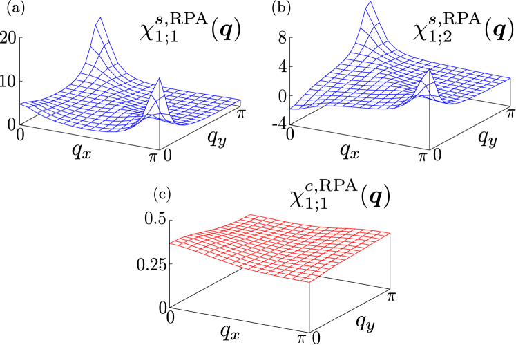
Figure 3: (color online) (a),(b) RPA spin susceptibilities $\chi^{s,{\rm RPA}}_{1;1}({{\bm{q}}})$ and $\chi^{s,{\rm RPA}}_{1;2}({{\bm{q}}})$ at $q_{z}=\pi$. Note that $\chi^{s,{\rm RPA}}_{2;2}({{\bm{Q}}}_{s})\approx 6$. (c) RPA charge susceptibility $\chi^{c,{\rm RPA}}_{1;1}({{\bm{q}}})$. We put $U=2.06$ eV and $J/U=1/9$.

III.2 Analysis of the Aslamazov-Larkin Vertex Correction for the orbital susceptibility

In the next stage, we study the charge susceptibility by taking the AL-VC into account, and derive the intra-unit-cell orbital order. In various two-dimensional multiorbital metals such as Fe-based and cuprate superconductors, the spin-fluctuation-driven orbital order and fluctuations are realized due to the large AL-VC for the charge channel Onari-SCVC ; Kontani-Raman ; Tsuchiizu-Ru1 . In this mechanism, very weak spin fluctuations give rise to the orbital order when the ratio $J/U$ is small, as observed in FeSe with ${\bar{J}}/{\bar{U}}\approx 0.1$ FeSe-Yamakawa ; Ishida-NMR ; Dresden-NMR . However, it is highly nontrivial whether the AL-VC is important or not in three-dimensional systems like Ti-oxypnictides. In this paper, we calculate the AL-VC in the three-dimensional model for the first time. We neglect the AL-VC for the spin channel and the Maki-Thompson VCs since they are negligible in various models Onari-SCVC ; FeSe-Yamakawa ; Yamakawa-CDW ; Tsuchiizu-CDW . We drop the feedback effect from ${\hat{\chi}}^{c}$ to ${\hat{X}}^{c}$ since its smallness has been verified in the present model, similarly to the case of the $d$-$p$ Hubbard model for cuprates Yamakawa-CDW . The expression for the AL-VC is given in Appendix A.

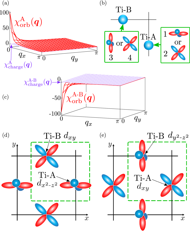
Figure 4: (color online) (a) $\chi^{\rm A}_{\rm orb}({{\bm{q}}})$ and $\chi^{\rm A}_{\rm charge}({{\bm{q}}})$ at $q_{z}=0$ obtained by including the AL-VC. We put $U=2.06$ eV and $J/U=1/9$. (b) Schematic intra-site orbital polarization. (c) $\chi^{\rm A\mbox{-}B}_{\rm orb}({{\bm{q}}})$ and $\chi^{\rm A\mbox{-}B}_{\rm charge}({{\bm{q}}})$ at $q_{z}=0$. (d),(e) Schematic intra-unit-cell nematic orbital order $(\Delta n_{x^{2}-z^{2}}^{\rm Ti\mbox{-}A},\Delta n_{xy}^{\rm Ti\mbox{-}A},\Delta n_{y^{2}-z^{2}}^{\rm Ti\mbox{-}B},\Delta n_{xy}^{\rm Ti\mbox{-}B})\propto\pm(1,-1,-1,1)$, which triggers the orthorhombic structural transition.

We present the numerical results obtained by including the AL-VC. The Stoner factors are $({\alpha}_{C},{\alpha}_{S})=(0.99,0.98)$ for $U=2.06$ eV and $J/U=1/9$ at $T=50$ meV. Figure 4 (a) shows the susceptibility of the orbital polarization at Ti-A site,

$$\chi^{\rm A}_{\rm orb}({{\bm{q}}}) \equiv \sum_{l,m=1}^{2}\chi^{c}_{l;m}({{\bm{q}}})\cdot(-1)^{l+m}$$ (3)

$$= \chi^{c}_{1;1}({{\bm{q}}})+\chi^{c}_{2;2}({{\bm{q}}})-2\chi^{c}_{1;2}({{\bm{q}}}),$$

at $q_{z}=0$. We see that the strong ferro-orbital fluctuations appear due to the AL-VC, which are absent in the RPA result in Fig. 3 (c). In contrast, the susceptibility of the charge density at Ti-A site, $\chi^{\rm A}_{\rm charge}({{\bm{q}}})\equiv\sum_{l,m=1}^{2}\chi^{c}_{l;m}({{\bm{q}}})=\chi^{c}_{1;1}({{\bm{q}}})+\chi^{c}_{2;2}({{\bm{q}}})+2\chi^{c}_{1;2}({{\bm{q}}})$, remains small as shown in Fig. 4 (a). These results means the emergence of the intra-site orbital polarization, $\Delta n_{1}\Delta n_{2}<0$ at Ti-A and $\Delta n_{3}\Delta n_{4}<0$ at Ti-B, as schematically shown in Fig. 4 (b). Here, $\Delta n_{l}$ is the modulation of the electron density on orbital $l$.

In addition, the inter-site orbital susceptibility between Ti-A and Ti-B,

$$\chi^{\rm A\mbox{-}B}_{\rm orb}({{\bm{q}}}) \equiv \sum_{l,m=1}^{2}\chi^{c}_{l;m+2}({{\bm{q}}})\cdot(-1)^{l+m}$$ (4)

$$= \chi^{c}_{1;3}({{\bm{q}}})+\chi^{c}_{2;4}({{\bm{q}}})-\chi^{c}_{1;4}({{\bm{q}}})-\chi^{c}_{2;3}({{\bm{q}}}),$$

has large negative peak at ${{\bm{q}}}={\bm{0}}$ as we show in Fig. 4 (c). In contrast, the inter-site charge susceptibility $\chi^{\rm A\mbox{-}B}_{\rm charge}({{\bm{q}}})\equiv\sum_{l,m=1}^{2}\chi^{c}_{l;m+2}({{\bm{q}}})$ is not enhanced at all. These results mean that the orbital polarization in the ordered state, $\Delta{\bm{n}}\equiv(\Delta n_{1},\Delta n_{2},\Delta n_{3},\Delta n_{4})$, is roughly proportional to $\pm(1,-1,-1,1)$.

More properly, the orbital polarization $\Delta{\bm{n}}$ is proportional to the form factor $\bm{f}$, which is given by the eigenvector of ${\hat{\Phi}}^{c}(q){\hat{\Gamma}}^{c}$ for the largest eigenvalue $\alpha_{c}$, as we discussed in Ref. Yamakawa-CDW . The obtained form factor for Fig. 4 is $\bm{f}=\pm(1.06,-0.94,-1.06,0.94)$. Thus, the predicted orbital patter are shown in Fig. 4 (d) or (e): When the electron densities for orbitals 1 and 4 in Fig. 4 (d) increase, the densities for other orbitals in (e) decrease. The predicted intra-unit-cell orbital order is consistent with the absence of the superlattice in BaTi₂(As,Sb)₂O in the nematic phase reported by the electron diffraction study Frandsen2014 ; Nozaki .

The charge pattern in Fig. 4 (d),(e) may be safely called orbital-selective charge order, since it is the spontaneous symmetry breaking among degenerate orbitals on different sites. (Two orbitals on the same Ti-ion are non-degenerated.) However, we call this charge pattern the orbital order for simplicity, since the net charge at Ti-A and that at Ti-B are almost equivalent.

III.3 Explanation for the intra-unit-cell orbital order due to the AL-VC

Here, we verify numerically that the intra- and inter-orbital fluctuations in Fig. 4 originates from the diagonal elements of the AL-VC; $X_{l;l}^{c}({\bm{0}})$ with $l=1\sim 4$. For $U=2.06$ eV, the diagonal elements of the AL-VCs are shown in Figs. 5 (a) and (b), in which $X_{1;1}^{c}({\bm{0}})=0.84$ and $X_{2;2}^{c}({\bm{0}})=0.49$ respectively. Then, the irreducible susceptibilities are $\Phi_{1;1}({\bm{0}})=1.21$ and $\Phi_{2;2}({\bm{0}})=0.75$. By taking only the diagonal AL-VCs into account in ${\hat{\Phi}}^{c}$, strong orbital fluctuations with the form factor ${\bm{f}}=\pm(1.04,-0.96,-1.04,0.96)$ appears at $U\approx 2.0$ eV.

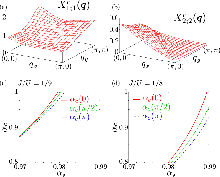
Figure 5: (color online) (a),(b) Obtained AL-VCs $X_{1;1}^{c}({{\bm{q}}})$ and $X_{2;2}^{c}({{\bm{q}}})$ at ${{\bm{q}}}_{z}=0$ for $J/U=1/9$. (c) ${\alpha}_{C}(q_{z})$ for $J/U=1/9$ and (d) ${\alpha}_{C}(q_{z})$ for $J/U=1/8$ as functions of ${\alpha}_{S}$.

Next, we present a mathematical explanation why the strong orbital fluctuations with the form factor ${\bm{f}}\propto(1,-1,-1,1)$ are obtained, which corresponds to the intra-unit-cell orbital order. To understand this nontrivial result, we put $\Phi_{l,l}({\bm{0}})=\Phi$ for $l=1,3$ and $\Phi_{l,l}({\bm{0}})=(1-x)\cdot\Phi$ for $l=2,4$, and other elements are zero for simplicity. We also put $U=U^{\prime}$ and $J=0$ for simplicity. Under this simplification, the largest eigenvalue of ${\hat{\Phi}}^{c}(q){\hat{\Gamma}}^{c}$ is doubly degenerate, and the corresponding form factors are ${\bm{f}}_{1}\propto(y,-1,-y,1)$ and ${\bm{f}}_{2}\propto(y,-1,y,-1)$, where $y\approx 1+x/4$ for $|x|\ll 1$, as we explain in Appendix B. This degeneracy of the form factor is lifted by the small inter-site components of $\Phi_{l;m}({\bm{0}})$ with $l\leq 2$ and $m\geq 3$. In the present model, the form factor ${\bm{f}}_{1}$ is selected mainly due to the negative $X^{c}_{1;3}({\bm{0}})$, as explained in Appendix B. Therefore, the intra-unit-cell orbital order with ${\bm{f}}_{1}\approx(1,-1,-1,1)$ is stably obtained without tuning model parameters.

In the present theory, the charge Stoner factor ${\alpha}_{C}$ is enlarged by the AL-VC, and the AL-VC increases near the magnetic critical point. Figures 5 (c) and (d) shows the charge Stoner factor for a fixed $q_{z}$, ${\alpha}_{C}(q_{z})$, as function of ${\alpha}_{S}$ for $J/U=1/9$ and $1/8$, respectively. In both cases, ${\alpha}_{C}(q_{z})$ at $q_{z}=0$ reaches unity for the smallest ${\alpha}_{S}$, meaning that the orbital order at ${{\bm{q}}}=(0,0,0)$ is realized. The orbital order should trigger the experimental orthorhombic structure transition at $T=T_{S}$.

III.4 Pseudo-gap formation in the orbital-ordered state

Below, we discuss the electronic states in the ordered state below $T_{S}$, by introducing the orbital-dependent potential energy $\Delta E_{l}$ ($l=1\sim 4$). The potential energy for the intra-unit-cell orbital order in Fig. 4 (d) or (e) is $\Delta{\bm{E}}_{\rm orbital}\equiv(\Delta E,-\Delta E,-\Delta E,\Delta E)$. In addition, we also discuss the intra-unit-cell charge order $\Delta{\bm{E}}_{\rm charge}\equiv(\Delta E,\Delta E,-\Delta E,-\Delta E)$. This possibility had been discussed in Ref. Frandsen2014 . We note that the orbital-ordered state in Fe-based superconductors ($n_{xz}\neq n_{yz}$) had been explained theoretically, by developing the self-consistent vertex correction (SC-VC) theory for the orbital-ordered state Onari-FeSe , and the experimental orbital polarization $E_{yz}-E_{xz}$ is $50\sim 60$ meV.

Figure 6 shows the DOS, $D({\epsilon})$, in the (a) orbital-ordered state and (b) charge-ordered state for $\Delta E=0\sim 0.4$ eV. To make comparison with experiments qualitatively, $\Delta E$ should be multiplied with the renormalization factor due to the self-energy, $z\equiv m_{\rm band\mbox{-}calc}/m^{*}\ (<1)$, although the value of $z$ is unknown in Ti-oxypnictides. (Note that $z^{-1}\approx 2\sim 10$ in Fe-based superconductors.) In (a), the DOS at the Fermi level, $D(0)$, decreases with $\Delta E>0$, and the pseudo-gap structure appears. In (b), in contrast, $D(0)$ is almost independent of $\Delta E$. The reason for the pseudo-gap formation in (a) is that both the electron-like FS around M point and hole-like FS around X point shrink with $\Delta E$, whereas only the latter shrinks in (b). The striking difference in the FS deformation is understood from the orbital character of the electron-like FS, as we discuss in Appendix C.

In Fig. 6 (c), we show the DOS for $\Delta{\bm{E}}\equiv(\Delta E,0,-\Delta E,0)[=(\Delta{\bm{E}}_{\rm orbital}+\Delta{\bm{E}}_{\rm charge})/2]$, which is also a possible nematic state suggested experimentally Frandsen2014 .

Experimentally, below $T_{S}$, the resistivity shows the upturn, and the uniform susceptibility is suppressed YajimaJPSJ2012 ; YajimaJPSJ2013 . Also, a pseudo-gap formation is indicated by ARPES below $T_{S}$ Tan ; Xu . Thus, the reduction of $D(0)$ due to the orbital order shown in Fig. 6 (a) is consistent with experimental results in Ti-oxypnictides.

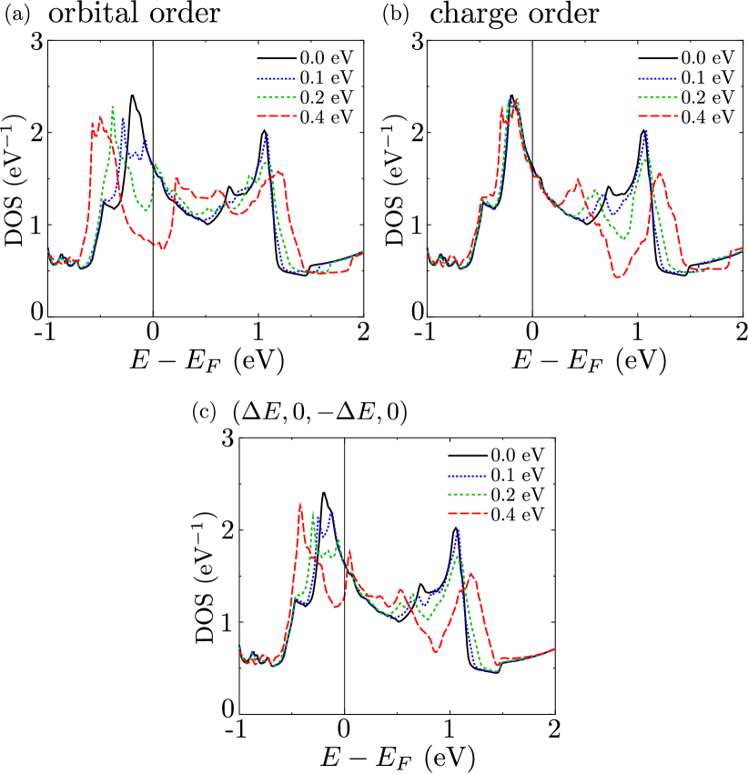
Figure 6: (color online) The DOSs for (a) orbital order state $\Delta{\bm{E}}_{\rm orbital}$, (b) charge order state $\Delta{\bm{E}}_{\rm charge}$, and (c) $\Delta{\bm{E}}\equiv(\Delta E,0,-\Delta E,0)$. The black, blue, green and red lines correspond to $\Delta E=0$, $0.1$, $0.2$, and $0.4$ eV respectively.

IV Discussions

We discuss the mechanism of the superconductivity in Ti-oxypnictides. Up to now, both the spin-fluctuation-mediated unconventional pairing Singh and the phonon-mediated conventional pairing Subedi mechanisms were proposed. The latter may be supported by the full-gap structure reported by the specific heat study in Ba_1-xNa_xTi₂Sb₂O Gooch . However, it is naturally expected that the orbital fluctuations near the orthorhombic phase would contribute to the pairing mechanism Kontani-RPA . This is our important future problem.

In the present AL-VC theory, the obtained wavevector of the orbital order is ${{\bm{q}}}=(0,0,0)$, which is consistent with the report in Ref. Frandsen2014 . On the other hand, the SC-VC theory explain the incommensurate orbital order at ${{\bm{q}}}_{c}=(\delta,0,0)$ in cuprate superconductors Yamakawa-CDW ; Tsuchiizu-CDW : ${{\bm{q}}}_{c}$ is equal to the wavevector connecting the neighboring hot spots. This fact indicates that the incommensurate orbital order might be realized in some Ti-oxypnictides, depending on the details of the bandstructure.

In Ref. Frandsen2014 , the authors discussed the nematic charge order driven by the nearest-neighbor Coulomb interaction $V$. At present, there is no first principles study for $V$. However, if $V$ were the origin of the nematic order, fine tuning of the parameters $V$ and $U$ is required to explain the development of spin fluctuations near $T_{S}$ in BaTi₂Sb₂O NMR . On the other hand, the coexistence of spin and orbital fluctuations is naturally explained by the strong orbital-spin interplay described by the AL-VC. The AL-VC mechanism explains the orbital-order in Fe-based superconductors Onari-SCVC and the nematic CDW order in cuprate superconductors Yamakawa-CDW . We stress that the importance of the AL-VC has been confirmed by the unbiased numerical study using the functional-renormalization-group theory Tsuchiizu-CDW ; Tsuchiizu-RG

In summary, we studied the origin of the nematic order without magnetization in Ti-oxypnictides based on the three-dimensional first-principles model. We predicted the formation of the intra-unit-cell orbital order in BaTi₂(As,Sb)₂O, which is driven by the orbital-spin interplay (AL-VC). The present intra-unit-cell orbital order can be confirmed experimentally by observing the shear modulus $C_{S}$ and the electron Raman spectroscopy for $B_{1g}$ channel, both of which are useful to observe the nematic fluctuations in Fe-based superconductors Kontani-Raman . The orbital order due to the AL-VC mechanism is expected to emerge not only in the two-dimensional high-$T_{\rm c}$ superconductors, but also in the three-dimensional multiorbital systems with moderate spin fluctuations such as Ti-oxypnictides. It would be an interesting future problem to clarify the role of the orbital fluctuations on the superconductivity.

Appendix A Numerical study of the AL-VC in three-dimensional systems

In the main text, we study the Aslamazov-Larkin vertex correction (AL-VC) in the three-dimensional 10-orbital Hubbard model for Ti-oxypnictides. To our knowledge, this is the first numerical study of the AL-VC in the three-dimensional multiorbital model.

In this model, we verified that the AL-VCs $X^{c}_{l,l^{\prime};m,m^{\prime}}(q)$ with $l\neq l^{\prime}$ or $m\neq m^{\prime}$ are negligibly small. Therefore, we calculate the AL-VC $X^{c}_{l,m}(q)\equiv X^{c}_{l,l;m,m}(q)$ in the present study. Its expression is given as

$$X^{c}_{l,m}(q) = \frac{T}{2}\sum_{p}\sum_{i_{1}\sim j_{4}}\Lambda_{ll,i_{1}i_{2},j_{1}j_{2}}(q;p)\Lambda^{\prime}_{mm,i_{3}i_{4},j_{3}j_{4}}(q;p)$$ (5)

$$\times\{3V^{s}_{i_{1}i_{2},i_{3}i_{4}}(p+q)V^{s}_{j_{1}j_{2},j_{3}j_{4}}(-p)$$

$$\hskip 11.38092pt+V^{c}_{i_{1}i_{2},i_{3}i_{4}}(p+q)V^{c}_{j_{1}j_{2},j_{3}j_{4}}(-p)\},$$

where the three-point vertex and spin (charge) channel interaction are given as

$$\!\!\!\!\!\!\!\!\Lambda_{ll,i_{1}i_{2},j_{1}j_{2}}(q;p)$$

$$\ \ \ \ \ \ =-T\sum_{k}G_{li_{1}}(k+q)G_{j_{2}l}(k)G_{i_{2}j_{1}}(k-p),$$ (6)

$$\!\!\!\!\!\!\!\!\Lambda^{\prime}_{mm,i_{3}i_{4},j_{3}j_{4}}(q;p)=\Lambda_{i_{3}j_{4},mj_{3},i_{4}m}(q;p)$$

$$\ \ \ \ \ \ \ \ \ \ \ \ \ \ \ \ \ \ \ \ \ \ +\Lambda_{j_{3}i_{4},mi_{3},j_{4}m}(q;-p-q),$$ (7)

$$\!\!\!\!\!\!\!\!{\hat{V}}^{s(c)}(q)={\hat{\Gamma}}^{s(c)}+{\hat{\Gamma}}^{s(c)}{\hat{\chi}}^{s(c)}(q){\hat{\Gamma}}^{s(c)}.$$ (8)

The diagrammatic expression of the AL-VC is shown in Fig. 7. Here, the second-order double counting terms in the AL-VC should be subtracted. In the present numerical study, we put $i_{1}=i_{2}$, $i_{3}=i_{4}$, $j_{1}=j_{2}$ and $j_{3}=j_{4}$ in eq. (5). This simplification is justified since $\chi^{s}_{l,l^{\prime};m,m^{\prime}}(q)$ is negligibly small for $l\neq l^{\prime}$ or $m\neq m^{\prime}$.

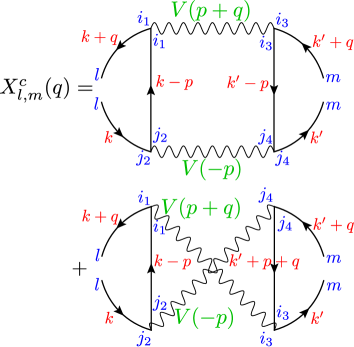
Figure 7: The diagram of AL-VC. $X^{c}_{l,m}(q)=X^{c}_{ll,mm}(q)$

In general, the AL-VC is less important in higher-dimensional systems, so it is significant to verify whether orbital fluctuations due to the AL-VC could develop in three-dimensional systems. In the presence of strong spin fluctuations, the AL-VC is scaled as

$$X^{c}({\bm{0}})\sim|\Lambda({\bm{0}};{{\bm{Q}}}_{s})|^{2}T\sum_{p}\{V^{s}({{\bm{p}}},0)\}^{2},$$ (9)

which is proportional to $|\Lambda({\bm{0}};{{\bm{Q}}}_{s})|^{2}T\xi_{\rm AF}^{4-d}$ when the spin fluctuations are $d$-dimensional, where $\xi_{\rm AF}$ is the antiferromagnetic correlation length. Therefore, the AL-VC is expected to be less important in the three-dimensional systems. Nonetheless, as revealed by the numerical study in the main text, the strong orbital fluctuations due to the AL-VC is realized in Ti-oxypnictides with three-dimensional FSs,

Appendix B Mathematical explanation for the intra-unit-cell orbital order due to the AL-VC

In the main text, we obtained the “intra-unit-cell orbital order” based on the BaTi₂(As,Sb)₂O model, by taking the AL-VC for ${\hat{\chi}}^{c}({{\bm{q}}})$ into account. The main origin of the orbital order is the large diagonal elements of the AL-VC $X_{l,l;l,l}({{\bm{q}}})$ at ${{\bm{q}}}={\bm{0}}$, which is enlarged near the magnetic critical point. Each $\chi_{l,l;m,m}^{c}({\bm{0}})$ ($l,m=1\sim 4$) has positive or negative large value, and the obtained orbital and charge susceptibilities are shown in Figs. 4 (a) and (c).

However, it is nontrivial that inter-site elements of $|\chi_{l,l;m,m}^{c}({\bm{0}})|$ with $l\leq 2$ and $m\geq 3$ are enlarged by the diagonal elements of the AL-VC and intra-site Coulomb interaction. We present the explanation for this nontrivial question based on the equation for the susceptibility (2).

$\chi^{0}_{l,l;m,m}$	$m=1$	$2$	$3$	$4$
$l=1$	$\ \bm{0.364}$	$-0.037$	$-0.034$	$0.094$
$2$		$\bm{0.258}$	$0.094$	$-0.046$
$3$			$\bm{0.364}$	$-0.037$
$4$				$\bm{0.258}$

$X^{c}_{l,l;m,m}$	$m=1$	$2$	$3$	$4$
$l=1$	$\ \bm{0.844}$	$\ 0.020$	$\bm{-0.252}$	$0.013$
$2$		$\bm{0.487}$	$0.013$	$0.099$
$3$			$\bm{0.844}$	$0.020$
$4$				$\bm{0.487}$

Table 1: Bare susceptibility $\chi_{l,l;m,m}^{0}$ (upper table) and AL-VC for the charge channel $X_{l,l;m,m}^{c}$ (lower table) at ${{\bm{q}}}={\bf 0}$ in the case of $U=2.06$ eV and $J/U=1/9$ at $T=50$ meV. The Stoner factors are $({\alpha}_{C},{\alpha}_{S})=(0.99,0.98)$. The numbers greater than 0.2 in magnitude are shown by bold fonts.

Table 1 shows the lists of the bare susceptibility $\chi_{l,l;m,m}^{0}$ (upper table) and AL-VC for the charge channel $X_{l,l;m,m}^{c}$ (lower table) at ${{\bm{q}}}={\bm{0}}$. The model parameters are equal to those used in the main text. It is found that the irreducible susceptibility $\Phi_{l,l;m,m}^{c}=\chi_{l,l;m,m}^{0}+X_{l,l;m,m}^{c}$ takes large value in magnitude only for $l=m=1\sim 4$ and for $(l,m)=(1,3)$. In addition, the elements $\Phi_{l,l^{\prime};m,m^{\prime}}$ with $l\neq l^{\prime}$ or $m\neq m^{\prime}$ are very small. In this case, the simplified equation for $\chi^{c}_{l,l;m,m}$, given by the $4\times 4$ matrix, is expressed as

$${\hat{\chi}}^{c(s)}=(1-{\hat{\Phi}}^{c(s)}{\hat{\Gamma}}^{c(s)})^{-1}{\hat{\Phi}}^{c(s)}.$$ (10)

In this section, we denote ${\chi}^{c(s)}_{l,m}\equiv\chi^{c(s)}_{l,l;m,m}$ and $\Phi_{l,m}^{c(s)}\equiv\Phi_{l,l;m,m}^{c(s)}$, and ${\Gamma}^{c(s)}_{l,m}\equiv\Gamma^{c(s)}_{l,l;m,m}$.

First, we analyze the intra-site charge susceptibility with $l,m\leq 2$ by neglecting the inter-site $\Phi_{l,m}^{c}$ ($l\leq 2$, $m\geq 3$). The $2\times 2$ charge susceptibility is given as

$$\begin{pmatrix}{\chi}_{1,1}^{c}&{\chi}_{1,2}^{c}\\ {\chi}_{2,1}^{c}&{\chi}_{2,2}^{c}\hfill\end{pmatrix} =({\hat{1}}-{\hat{C}}_{2})^{-1}\begin{pmatrix}\Phi_{1,1}^{c}&\Phi_{1,2}^{c}\\ \Phi_{2,1}^{c}&\Phi_{2,2}^{c}\end{pmatrix},$$ (11)

$${\hat{C}}_{2} =\begin{pmatrix}\Phi_{1,1}^{c}&\Phi_{1,2}^{c}\\ \Phi_{2,1}^{c}&\Phi_{2,2}^{c}\end{pmatrix}\!\!\begin{pmatrix}-U&-2U^{\prime}+J\\ -2U^{\prime}+J&-U\end{pmatrix}.$$ (12)

The maximum eigenvalue of $\displaystyle{\hat{C}}_{2}$ gives the charge Stoner factor ${\alpha}_{C}$, and its eigenvector gives the form factor ${\bm{g}}$ at ${\alpha}_{C}=1$. (Note that $\displaystyle{\hat{C}}_{2}$ is not Hermitian.) For simplicity, we examine the case of $\Phi_{l,m}^{c}=0$ for $l\neq m$, and $U^{\prime}=U$ and $J=0$. In this case, the charge Stoner factor is ${\alpha}_{C}=\frac{U}{2}[-(\Phi_{1,1}^{c}+\Phi_{2,2}^{c})+\sqrt{{\Phi_{1,1}^{c}}^{2}+{\Phi_{2,2}^{c}}^{2}+14{\Phi_{1,1}^{c}}{\Phi_{2,2}^{c}}}]\ (>0)$, and the form factor is ${\bm{g}}\propto(-{\Phi_{1,1}^{c}}+{\Phi_{2,2}^{c}}+\sqrt{{\Phi_{1,1}^{c}}^{2}+{\Phi_{2,2}^{c}}^{2}+14{\Phi_{1,1}^{c}}{\Phi_{2,2}^{c}}},\ -4{\Phi_{2,2}^{c}})$. When $\Phi_{2,2}=(1-x)\Phi_{1,1}$ and $|x|\ll 1$, the form factor is simplified as ${\bm{g}}\propto(y,-1)$, where $y=(\sqrt{1-x+x^{2}/16}-x/4)/(1-x)\approx 1+x/4$.

For the $4\times 4$ charge susceptibility in Eq. (10), the charge Stoner factor and the form factor are respectively given by the maximum eigenvalue and its eigenvector of the following $4\times 4$ matrix:

$${\hat{C}}_{4} =\begin{pmatrix}{\hat{C}}_{2}&{\hat{C}}_{2}^{\prime}\\ {\hat{C}}_{2}^{\prime\prime}&{\hat{C}}_{2}\end{pmatrix},$$ (13)

$${\hat{C}}_{2}^{\prime} =\begin{pmatrix}\Phi_{1,3}^{c}&\Phi_{1,4}^{c}\\ \Phi_{2,3}^{c}&\Phi_{2,4}^{c}\end{pmatrix}\!\!\begin{pmatrix}-U&-2U^{\prime}+J\\ -2U^{\prime}+J&-U\end{pmatrix},$$ (14)

$${\hat{C}}_{2}^{\prime\prime} =\begin{pmatrix}\Phi_{3,1}^{c}&\Phi_{4,1}^{c}\\ \Phi_{3,2}^{c}&\Phi_{4,2}^{c}\end{pmatrix}\!\!\begin{pmatrix}-U&-2U^{\prime}+J\\ -2U^{\prime}+J&-U\end{pmatrix}.$$ (15)

At ${{\bm{q}}}=0$, the relation ${\hat{C}}_{2}^{\prime}={\hat{C}}_{2}^{\prime\prime}$ holds, and the form factors are $({\bm{g}},\pm{\bm{g}})$ when ${\hat{C}}_{2}^{\prime}=0$. This degeneracy of the form factor is lifted in the presence of small ${\hat{C}}_{2}^{\prime}$, and the form factor is given as ${\bm{f}}\approx({\bm{g}},-{\bm{g}})$ when the inner product $({\bm{g}},{\hat{C}}_{2}^{\prime}{\bm{g}})$ is negative, which is satisfied in the present numerical study due to the large negative $X_{1,1;3,3}^{c}({\bm{0}})$ in Table 1.

To summarize, we presented a mathematical explanation why the orbital-order with the form factor ${\bm{f}}\sim(1,-1,-1,1)$, which corresponds to the numerical results in Figs. 4 (a) and (c), is universally obtained in the present numerical study.

Next, we analyze the intra-site spin susceptibility with $l,m\leq 2$ by neglecting the inter-site $\Phi_{l,m}^{s}$ ($l\leq 2$, $m\geq 3$). The $2\times 2$ spin susceptibility is given as

$$\begin{pmatrix}{\chi}_{1,1}^{s}&{\chi}_{1,2}^{s}\\ {\chi}_{2,1}^{s}&{\chi}_{2,2}^{s}\hfill\end{pmatrix} =({\hat{1}}-{\hat{S}}_{2})^{-1}\begin{pmatrix}\Phi_{1,1}^{s}&\Phi_{1,2}^{s}\\ \Phi_{2,1}^{s}&\Phi_{2,2}^{s}\end{pmatrix},$$ (16)

$${\hat{S}}_{2} =\begin{pmatrix}\Phi_{1,1}^{s}&\Phi_{1,2}^{s}\\ \Phi_{2,1}^{s}&\Phi_{2,2}^{s}\end{pmatrix}\!\!\begin{pmatrix}U&J\\ J&U\end{pmatrix},$$ (17)

where $\Phi_{l,m}^{s}({{\bm{q}}})\approx\chi_{l,m}^{0}({\bm{q}})$ is satisfied since the AL-VC for the spin channel is small. Since $J\ll U$, only the orbital diagonal elements of the spin susceptibility ${\chi}_{l,m}^{s}$ are enlarged. The spin Stoner factor is obtained as ${\alpha}_{S}=\frac{U}{2}[(\Phi_{1,1}^{s}+\Phi_{2,2}^{s})+\sqrt{(\Phi_{1,1}^{s}-\Phi_{2,2}^{s})^{2}+4(J/U)^{2}\Phi_{1,1}^{s}\Phi_{2,2}^{s}}]$ when $\Phi_{l,m}^{s}$ with $l\neq m$ is negligible.

In the RPA or FLEX approximation (${\hat{\Phi}}^{s}={\hat{\Phi}}^{c}$), the relation ${\alpha}_{C}\leq{\alpha}_{S}$ holds at any ${{\bm{q}}}$ for $J\geq 0$, according to the obtained expressions for ${\alpha}_{C}$ and ${\alpha}_{S}$. Nonetheless, the opposite relation ${\alpha}_{C}>{\alpha}_{S}$ is obtained in the present study thanks to the charge channel AL-VC. Therefore, the “orbital order without magnetization” is explained by the present orbital-spin fluctuation theory with including the AL-VC.

Appendix C Fermi surface deformation due to intra-unit-cell orders

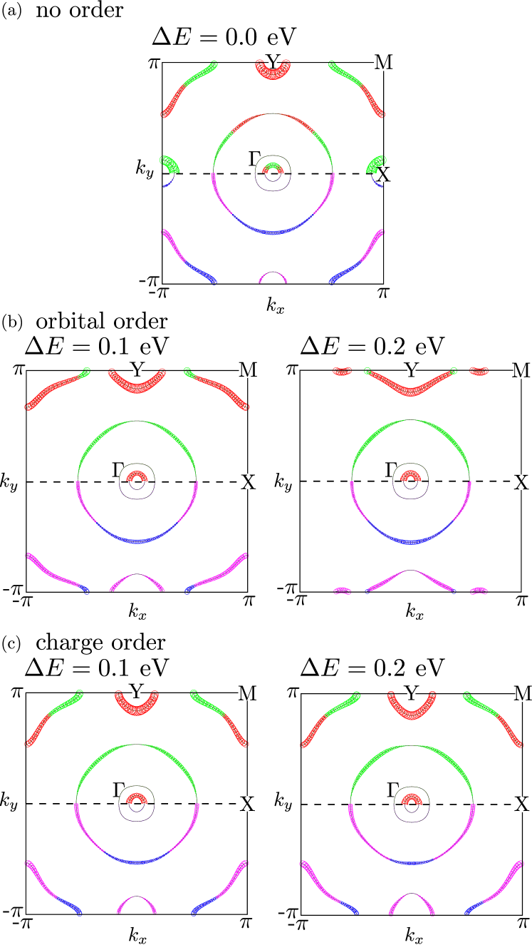
Figure 8: (a) The FSs in the $k_{z}=0$ plane in the absence of the orbital or charge order. The weights of the 1-, 2-, 3-, 4-orbitals are shown by the red, blue, green, and purple circles, respectively. The weights of the 1,3-orbitals (2,4-orbitals) are shown in the upper (lower) Brillouin zone. (b) The FSs under the orbital order with $\Delta E=0.1$ eV and $0.2$ eV. (c) The FSs under the charge order with $\Delta E=0.1$ eV and $0.2$ eV.

Here, we examine the orbital character of the FSs in detail, and discuss the FS deformation under the orbital and charge orders. Figure 8 (a) shows the FSs of the original tight-binding model in the $k_{z}=0$ plane. The weights of the 1,3-orbitals (2,4-orbitals) are shown in the upper (lower) Brillouin zone.

First, we calculate the FS deformation under the intra-unit-cell orbital order, by introducing the potential $\Delta{\bm{E}}_{\rm orbital}\equiv(\Delta E,-\Delta E,-\Delta E,\Delta E)$. Figure 8 (b) shows the FSs for $\Delta E=0.1$ eV and $0.2$ eV. In this case, the hole-FS around the X-point, which is mainly composed of the 3-orbital (green), disappears for $\Delta E\geq 0.1$ eV. In addition, the electron-FS around the M-point, mainly composed by (1+4)-orbital [(2+3)-orbital] near the $k_{x}=\pi$ [$k_{y}=\pi$] Brillouin zone boundary, disappears for $\Delta E\geq 0.2$ eV. For this reason, the pseudo-gap structure appears in the DOS at the Fermi level, as shown in Fig. 5 (a) in the main text.

Next, we calculate the FS deformation under the intra-unit-cell charge order with $\Delta{\bm{E}}_{\rm charge}\equiv(\Delta E,\Delta E,-\Delta E,-\Delta E)$. Figure 8 (c) shows the FSs for $\Delta E=0.1$ eV and $0.2$ eV. Then, the hole-FS around the X-point disappears for $\Delta E\geq 0.1$ eV, similarly to Fig. 8 (b). However, in contrast, the electron-FS around the M-point still exists for $\Delta E=0.2$ eV, since the potential on the (1+4)-orbital and that on the (2+3)-orbital cancel in the case of the charge order. For this reason, the DOS at the Fermi level is insensitive to $\Delta E$, as shown in Fig. 5 (b) in the main text.

According to the ARPES study for Na₂Ti₂Sb₂O, the pseudo-gap appears around the X-point Tan . This result is consistent with the FS deformation due to orbital order in Fig. 8 (b) as well as that due to the charge order in Fig. 8 (c). To distinguish between the orbital order and charge order, the ARPES study around the M-point is required.

References

- (1) R. M. Fernandes, L. H. VanBebber, S. Bhattacharya, P. Chandra, V. Keppens, D. Mandrus, M. A. McGuire, B. C. Sales, A. S. Sefat, and J. Schmalian, Phys. Rev. Lett. 105, 157003 (2010).
- (2) F. Wang, S. Kivelson, and D.-H. Lee, arXiv:1501.00844.
- (3) A.V. Chubukov, R.M. Fernandes, and Joerg Schmalian, Phys. Rev. B 91, 201105 (2015).
- (4) R. Yu, and Q. Si, Phys. Rev. Lett. 115, 116401 (2015); J. K. Glasbrenner, I. I. Mazin, H. O. Jeschke, P. J. Hirschfeld, and R. Valenti, Nature Physics 11, 935 (2015).
- (5) F. Krüger, S. Kumar, J. Zaanen, J. van den Brink, Phys. Rev. B 79, 054504 (2009).
- (6) W. Lv, J. Wu, and P. Phillips, Phys. Rev. B 80, 224506 (2009).
- (7) C.-C. Lee, W.-G. Yin, and W. Ku, Phys. Rev. Lett. 103, 267001 (2009).
- (8) S. Onari and H. Kontani, Phys. Rev. Lett. 109, 137001 (2012).
- (9) S. Onari, Y. Yamakawa, and H. Kontani, Phys. Rev. Lett. 112, 187001 (2014).
- (10) S. Onari and H. Kontani, Iron-Based Superconductivity, (ed. P.D. Johnson, G. Xu, and W.-G. Yin, Springer-Verlag Berlin and Heidelberg GmbH & Co. K (2015)).
- (11) K. Jiang, J. Hu, H. Ding, and Z. Wang, arXiv:1508.00588.
- (12) Y. Yamakawa and H. Kontani, Phys. Rev. Lett. 114, 257001 (2015).
- (13) M. Tsuchiizu, Y. Yamakawa and H. Kontani, arXiv:1508.07218.
- (14) J. C. S. Davis and D.-H. Lee, Proc. Natl. Acad. Sci. USA, 110, 17623 (2013).
- (15) E. Berg, E. Fradkin, S. A. Kivelson, and J. M. Tranquada, New J. Phys. 11, 115004 (2009).
- (16) Y. Wang and A.V. Chubukov, Phys. Rev. B 90, 035149 (2014).
- (17) M.A. Metlitski and S. Sachdev, New J. Phys. 12, 105007 (2010); S. Sachdev and R. La Placa, Phys. Rev. Lett. 111, 027202 (2013).
- (18) T. Yajima, K. Nakano, F. Takeiri, T. Ono, Y. Hosokoshi, Y, Matsushita, J. Hester, Y. Kobayashi, and H. Kageyama, J. Phys. Soc. Jpn. 81, 103706 (2012).
- (19) T. Yajima, K. Nakano, F. Takeiri, Y. Nozaki, Y. Kobayashi, and H. Kageyama, J. Phys. Soc. Jpn. 82, 033705 (2013).
- (20) H.-F. Zhai, W.-H. Jiao, Y.-L. Sun, J.-K. Bao, H. Jiang, X.-J. Yang, Z.-T. Tang, Q. Tao, X.-F. Xu, Y.-K. Li, C. Cao, J.-H. Dai, Z.-A. Xu, and G.-H. Cao, Phys. Rev. B 87, 100502(R) (2013).
- (21) X.F. Wang, Y.J. Yan, J.J. Ying, Q.J. Li, M. Zhang, N. Xu and X.H. Chen, J. Phys.: Condens. Matter 22, 075702 (2010).
- (22) S. Kitagawa, K. Ishida, K. Nakano, T. Yajima, and H. Kageyama, Phys. Rev. B 87, 060510(R) (2013).
- (23) F.von Rohr, A. Schilling, R. Nesper, C. Baines, and M. Bendele, Phys. Rev. B 88, 140501(R) (2013).
- (24) B. A. Frandsen, E.S. Bozi, H. Hu, Y. Zhu, Y. Nozaki, H. Kageyama, Y.J. Uemura, W.-G. Yin, S.J.L. Billinge, Nature Communications 5, 5761 (2014).
- (25) Y. Nozaki, K. Nakano, T. Yajima, H. Kageyama, B. Frandsen, L. Liu, S. Cheung, T. Goko, Y. J. Uemura, T. S. J. Munsie, T. Medina, G. M. Luke, J. Munevar, D. Nishio-Hamane, and C. M. Brown, Phys. Rev. B 88, 214506 (2013).
- (26) K. Fujita et al., Proc. Natl. Acad. Sci. USA, 110, E3026 (2014).
- (27) A. Subedi, Phys. Rev. B 87, 054506 (2013).
- (28) X.-L. Yu, D.-Y. Liu, Y.-M. Quan, T. Jia, H.-Q. Lin, and L.-J. Zou, J. Appl. Phys. 115, 17A924 (2014).
- (29) D.J. Singh, New J. Phys. 14, 123003 (2012).
- (30) T. Miyake, K. Nakamura, R. Arita, and M. Imada, J. Phys. Soc. Jpn. 79, 044705 (2010).
- (31) H. Kontani and Y. Yamakawa, Phys. Rev. Lett. 113, 047001 (2014).
- (32) M. Tsuchiizu, Y. Ohno, S. Onari, and H. Kontani, Phys. Rev. Lett. 111, 057003 (2013).
- (33) Y. Yamakawa, S. Onari and H. Kontani, arXiv:1509.01161.
- (34) A. E. Böhmer, P. Burger, F. Hardy, T. Wolf, P. Schweiss, R. Fromknecht, M. Reinecker, W. Schranz, and C. Meingast, Phys. Rev. Lett. 112, 047001 (2014).
- (35) A.E. Böhmer, T. Arai, F. Hardy, T. Hattori, T. Iye, T. Wolf, H.v. Lohneysen, K. Ishida, and C. Meingast, Phys. Rev. Lett. 114, 027001 (2015).
- (36) S.-H. Baek, D. V. Efremov, J. M. Ok, J. S. Kim, Jeroen van den Brink, and B. Buchner, Nature Mater. 14, 210 (2015).
- (37) M. Yi, D. Lu, J.-H. Chu, J. G. Analytis, A. P. Sorini, A. F. Kemper, B. Moritz, S.-K. Mo, R. G. Moore, M. Hashimoto, W.-S. Lee, Z. Hussain, T. P. Devereaux, I. R. Fisher, and Z.-X. Shen, Proc. Natl. Acad. Sci. USA 108, 6878 (2011).
- (38) T. Shimojima, Y. Suzuki, T. Sonobe, A. Nakamura, M. Sakano, J. Omachi, K. Yoshioka, M. Kuwata-Gonokami, K. Ono, H. Kumigashira, A. E. Böhmer, F. Hardy, T. Wolf, C. Meingast, H. v. Lohneysen, H. Ikeda, and K. Ishizaka, Phys. Rev. B 90, 121111(R) (2014).
- (39) S. Onari, Y. Yamakawa, and H. Kontani, arXiv:1509.01172.
- (40) S. Y. Tan, J. Jiang, Z. R. Ye, X. H. Niu, Y. Song, C. L. Zhang, P. C. Dai, B. P. Xie, X. C. Lai, and D. L. Feng, Sci. Rep. 5, 9515 (2015).
- (41) H. C. Xu, M. Xu, R. Peng, Y. Zhang, Q. Q. Ge, F. Qin, M. Xia, J. J. Ying, X. H. Chen, X. L. Yu, L. J. Zou, M. Arita, K. Shimada, M. Taniguchi, D. H. Lu, B. P. Xie, and D. L. Feng, Phys. Rev. B 89, 155108 (2014).
- (42) M. Gooch, P. Doan, Z. Tang, B. Lo renz, A.M. Guloy, and P.C.W. Chu, Phys. Rev. B 88, 064510 (2013).
- (43) H. Kontani and S. Onari, Phys. Rev. Lett. 104, 157001 (2010).
- (44) M. Tsuchiizu, Y. Ohno, S. Onari, and H. Kontani, Phys. Rev. Lett. 111, 057003 (2013).