Approximate option pricing in the Lévy Libor model

Abstract.

In this paper we consider the pricing of options on interest rates such as caplets and swaptions in the Lévy Libor model developed by EberleinOezkan05. This model is an extension to Lévy driving processes of the classical log-normal Libor market model (LMM) driven by a Brownian motion. Option pricing is significantly less tractable in this model than in the LMM due to the appearance of stochastic terms in the jump part of the driving process when performing the measure changes which are standard in pricing of interest rate derivatives. To obtain explicit approximation for option prices, we propose to treat a given Lévy Libor model as a suitable perturbation of the log-normal LMM. The method is inspired by recent works by CernyDenklKallsen13 and MenasseTankov15. The approximate option prices in the Lévy Libor model are given as the corresponding LMM prices plus correction terms which depend on the characteristics of the underlying Lévy process and some additional terms obtained from the LMM model.

Key words: Libor market model, caplet, swaption, Lévy Libor model, asymptotic approximation.

1. Introduction

The goal of this paper is to develop explicit approximations for option prices in the Lévy Libor model introduced by EberleinOezkan05. In particular, we shall be interested in price approximations for caplets, whose pay-off is a function of only one underlying Libor rate and swaptions, which can be regarded as options on a “basket” of multiple Libor rates of different maturities.

A full-fledged model of Libor rates such as the Lévy Libor model is typically used for the purposes of pricing and risk management of exotic interest rate products. The prices and hedge ratios must be consistent with the market-quoted prices of liquid options, which means that the model must be calibrated to the available prices / implied volatilities of caplets and swaptions. To perform such a calibration efficiently, one therefore needs explicit formulas or fast numerical algorithms for caplet and swaption prices.

Computation of option prices in the Lévy Libor model to arbitrary precision is only possible via Monte Carlo. Efficient simulation algorithms suitable for pricing exotic options have been proposed in [Kohatsu-Higa and TankovKohatsu-Higa and Tankov2010, Papapantoleon, Schoenmakers, and SkovmandPapapantoleon et al.2012], however, these Monte Carlo algorithms are probably not an option for the purposes of calibration because the computation is still too slow due to the presence of both discretization and statistical error.

EberleinOezkan05, Kluge05 and [Belomestny and SchoenmakersBelomestny and Schoenmakers2011] propose fast methods for computing caplet prices which are based on Fourier transform inversion and use the fact that the characteristic function of many parametric Lévy processes is known explicitly. Since in the Lévy Libor model, the Libor rate $L^{k}$ is not a geometric Lévy process under the corresponding probability measure $\mathbb{Q}^{T_{k}}$, unless $k=n$ (see Remark 3.1 below for details), using these methods for $k<n$ requires an additional approximation (some random terms appearing in the compensator of the jump measure of $L^{k}$ are approximated by their values at time $t=0$, a method known as freezing).

In this paper we take an alternative route and develop approximate formulas for caplets and swaptions using asymptotic expansion techniques. Inspired by methods used in CernyDenklKallsen13 and MenasseTankov15 (see also [Benhamou, Gobet, and MiriBenhamou et al.2009, Benhamou, Gobet, and MiriBenhamou et al.2010] for related expansions “around a Black-Scholes proxy” in other models), we consider a given Lévy Libor model as a perturbation of the log-normal LMM. Starting from the driving Lévy process $(X_{t})_{t\geq 0}$ of the Lévy Libor model, assumed to have zero expectation, we introduce a family of processes $X^{\alpha}_{t}=\alpha X_{t/\alpha^{2}}$ parameterized by $\alpha\in(0,1]$, together with the corresponding family of Lévy Libor models. For $\alpha=1$ one recovers the original Lévy Libor model. When $\alpha\to 0$, the family $X^{\alpha}$ converges weakly in Skorokhod topology to a Brownian motion, and the option prices in the Lévy Libor model corresponding to the process $X^{\alpha}$ converge to the prices in the log-normal LMM. The option prices in the original Lévy Libor model can then be approximated by their second-order expansions in the parameter $\alpha$, around the value $\alpha=0$. This leads to an asymptotic approximation formula for a derivative price expressed as a linear combination of the derivative price stemming from the LMM and correction terms depending on the characteristics of the driving Lévy process. The terms of this expansion are often much easier to compute than the option prices in the Lévy Libor model. In particular, we shall see the expansion for caplets is expressed in terms of the derivatives of the standard Black’s formula, and the various terms of the expansion for swaptions can be approximated using one of the many swaption approximations for the log-normal LMM available in the literature.

This paper is structured as follows. In Section 2 we briefly review the Lévy Libor model. In Section 3 we show how the prices of European-style options may be expressed as solutions of partial integro-differential equations (PIDE). These PIDEs form the basis of our asymptotic method, presented in detail in Section 4. Finally, numerical illustrations are provided in Section 5.

2. Presentation of the model

In this section we present a slight modification of the Lévy Libor model by EberleinOezkan05, which is a generalization, based on Lévy processes, of the Libor market model driven by a Brownian motion, introduced by SandmannSondermannMiltersen95, BraceGatarekMusiela97 and MiltersenSandmannSondermann97.

Let a discrete tenor structure $0\leq T_{0}<T_{1}<\ldots<T_{n}$ be given, and set $\delta_{k}:=T_{k}-T_{k-1}$, for $k=1,\ldots,n$. We assume that zero-coupon bonds with maturities $T_{k}$, $k=0,\ldots,n$, are traded in the market. The time-$t$ price of a bond with maturity $T_{k}$ is denoted by $B_{t}(T_{k})$ with $B_{T_{k}}(T_{k})=1$.

For every tenor date $T_{k}$, $k=1,\ldots,n$, the forward Libor rate $L_{t}^{k}$ at time $t\leq T_{k-1}$ for the accrual period $[T_{k-1},T_{k}]$ is a discretely compounded interest rate defined as

$$L_{t}^{k}:=\frac{1}{\delta_{k}}\left(\frac{B_{t}(T_{k-1})}{B_{t}(T_{k})}-1\right).$$ (2.1)

For all $t>T_{k-1}$, we set $L_{t}^{k}:=L_{T_{k-1}}^{k}$.

To set up the Libor model, one needs to specify the forward Libor rates $L_{t}^{k}$, $k=1,\ldots,n$, such that each Libor rate $L^{k}$ is a martingale with respect to the corresponding forward measure $\mathbb{Q}^{T_{k}}$ using the bond with maturity $T_{k}$ as numéraire. We recall that the forward measures are interconnected via the Libor rates themselves and hence each Libor rate depends also on some other Libor rates as we shall see below. More precisely, assuming that the forward measure $\mathbb{Q}^{T_{n}}$ for the most distant maturity $T_{n}$ (i.e. with numéraire $B(T_{n})$) is given, the link between the forward measure $\mathbb{Q}^{T_{k}}$ and $\mathbb{Q}^{T_{n}}$ is provided by

$$\frac{d\mathbb{Q}^{T_{k}}}{d\mathbb{Q}^{T_{n}}}\Big{|}_{\mathcal{F}_{t}} =\frac{B_{t}(T_{k})}{B_{t}(T_{n})}\frac{B_{0}(T_{n})}{B_{0}(T_{k})}=\prod_{j=k+1}^{n}\frac{1+\delta_{j}L^{j}_{t}}{1+\delta_{j}L^{j}_{0}},$$ (2.2)

for every $k=1,\ldots,n-1$. The forward measure $\mathbb{Q}^{T_{n}}$ is referred to as the terminal forward measure.

2.1. The driving process

Let us denote by $(\Omega,{\mathcal{F}},\mathbf{F}=({\mathcal{F}}_{t})_{0\leq t\leq T^{*}},\mathbb{Q}^{T_{n}})$ a complete stochastic basis and let $X$ be an $\mathbb{R}^{d}$-valued Lévy process $(X_{t})_{0\leq t\leq T^{*}}$ on this stochastic basis with Lévy measure $F$ and diffusion matrix $c$. The filtration $\mathbf{F}$ is generated by $X$ and $\mathbb{Q}^{T_{n}}$ is the forward measure associated with the date $T_{n}$, i.e. with the numeraire $B_{t}(T_{n})$. The process $X$ is assumed without loss of generality to be driftless under $\mathbb{Q}^{T_{n}}$.

Moreover, we assume that $\int_{|z|>1}|z|F(dz)<\infty$. This implies in addition that $X$ is a special semimartingale and allows to choose the truncation function $h(z)=z$, for $z\in\mathbb{R}^{d}$. The canonical representation of $X$ is given by

$$X_{t}=\sqrt{c}W_{t}^{T_{n}}+\int_{0}^{t}\int_{\mathbb{R}^{d}}z(\mu-\nu^{T_{n}})(ds,dz),$$ (2.3)

where $W^{T_{n}}=(W^{T_{n}}_{t})_{0\leq t\leq T_{n}}$ denotes a standard $d$-dimensional Brownian motion with respect to the measure $\mathbb{Q}^{T_{n}}$, $\mu$ is the random measure of jumps of $X$ and $\nu^{T_{n}}(ds,dz)=F(dz)ds$ is the $\mathbb{Q}^{T_{n}}$-compensator of $\mu$.

2.2. The model

Denote by $L=(L^{1},\ldots,L^{n})^{\top}$ the column vector of forward Libor rates. We assume that under the terminal measure $\mathbb{Q}^{T_{n}}$, the dynamics of $L$ is given by the following SDE

$$dL_{t}=L_{t-}(b(t,L_{t})dt+\Lambda(t)dX_{t}),$$ (2.4)

where $b(t,L_{t})$ is the drift term and $\Lambda(t)$ a deterministic $n\times d$ volatility matrix. We write $\Lambda(t)=(\lambda^{1}(t),\ldots,\lambda^{n}(t))^{\top}$, where $\lambda^{k}(t)$ denotes the $d$-dimensional volatility vector of the Libor rate $L^{k}$ and assuming that $\lambda^{k}(t)=0$, for $t>T_{k-1}$.

One typically assumes that the jumps of $X$ are bounded from below, i.e. $\Delta X_{t}>C$, for all $t\in[0,T^{*}]$ and for some strictly negative constant $C$, which is chosen such that it ensures the positivity of the Libor rates given by (2.4).

The drift $b(t,L_{t})=(b^{1}(t,L_{t}),\ldots,b^{n}(t,L_{t}))$ is determined by the no-arbitrage requirement that $L^{k}$ has to be a martingale with respect to $\mathbb{Q}^{T_{k}}$, for every $k=1,\ldots,n$. This yields

$$b^{k}(t,L_{t}) =-\sum_{j=k+1}^{n}\frac{\delta_{j}L_{t}^{j}}{1+\delta_{j}L_{t}^{j}}\langle\lambda^{k}(t),c\,\lambda^{j}(t)\rangle$$ (2.5)

$$+\int_{\mathbb{R}^{d}}\langle\lambda^{k}(t),z\rangle\left(1-\prod_{j=k+1}^{n}\left(1+\frac{\delta_{j}L_{t}^{j}\langle\lambda^{j}(t),z\rangle}{1+\delta_{j}L_{t}^{j}}\right)\right)F(dz).$$

The above drift condition follows from (2.2) and Girsanov’s theorem for semimartingales noticing that

$$dL_{t}^{k} =L_{t-}^{k}(b^{k}(t,L_{t})dt+\lambda^{k}(t)dX_{t})$$

$$=L_{t-}^{k}\lambda^{k}(t)dX^{T_{k}}_{t},$$

where

$$X^{T_{k}}_{t}=\sqrt{c}W_{t}^{T_{k}}+\int_{0}^{t}\int_{\mathbb{R}^{d}}z(\mu-\nu^{T_{k}})(ds,dz)$$ (2.6)

is a special semimartingale with a $d$-dimensional $\mathbb{Q}^{T_{k}}$-Brownian motion $W^{T_{k}}$ given by

$$dW_{t}^{T_{k}}:=dW_{t}^{T_{n}}-\sqrt{c}\left(\sum_{j=k+1}^{n}\frac{\delta_{j}L_{t}^{j}}{1+\delta_{j}L_{t}^{j}}\lambda^{j}(t)\right)dt$$ (2.7)

and the $\mathbb{Q}^{T_{k}}$-compensator $\nu^{T_{k}}$ of $\mu$ given by

$$\nu^{T_{k}}(dt,dz) := \prod_{j=k+1}^{n}\left(1+\frac{\delta_{j}L_{t-}^{j}}{1+\delta_{j}L_{t-}^{j}}\langle\lambda^{j}(t),z\rangle\right)\nu^{T_{n}}(dt,dz)$$

$$= \prod_{j=k+1}^{n}\left(1+\frac{\delta_{j}L_{t}^{j}}{1+\delta_{j}L_{t}^{j}}\langle\lambda^{j}(t),z\rangle\right)F(dz)dt$$

$$= F^{T_{k}}_{t}(dz)dt$$

with

$$F^{T_{k}}_{t}(dz):=\prod_{j=k+1}^{n}\left(1+\frac{\delta_{j}L_{t}^{j}}{1+\delta_{j}L_{t}^{j}}\langle\lambda^{j}(t),z\rangle\right)F(dz).$$ (2.9)

Equalities (2.7) and (2.2), and consequently also the drift condition (2.5), are implied by Girsanov’s theorem for semimartingales applied first to the measure change from $\mathbb{Q}^{T_{n}}$ to $\mathbb{Q}^{T_{n-1}}$ and then proceeding backwards. We refer to [Proposition 2.6]Kallsen06 for a version of Girsanov’s theorem that can be directly applied in this case. Note that the random terms $\frac{\delta_{j}L_{t}^{j}}{1+\delta_{j}L_{t}^{j}}$ appear in the measure change due to the fact that for each $j=n,n-1,\ldots,1$ we have

$$d(1+\delta_{j}L_{t}^{j})=(1+\delta_{j}L_{t-}^{j})\left(\frac{\delta_{j}L_{t-}^{j}}{1+\delta_{j}L_{t-}^{j}}b^{j}(t,L_{t})dt+\frac{\delta_{j}L_{t-}^{j}}{1+\delta_{j}L_{t-}^{j}}\lambda^{j}(t)dX_{t}\right),$$ (2.10)

We point out that the predictable random terms $\frac{\delta_{j}L_{t-}^{j}}{1+\delta_{j}L_{t-}^{j}}$ can be replaced with $\frac{\delta_{j}L_{t}^{j}}{1+\delta_{j}L_{t}^{j}}$ in equalities (2.5), (2.7) and (2.2) due to absolute continuity of the characteristics of $X$.

Therefore, the vector process of Libor rates $L$, given in (2.4)

with the drift (2.5), is a time-inhomogeneous Markov process and its infinitesimal generator under $\mathbb{Q}^{T_{n}}$ is given by

$$\mathcal{A}_{t}f(x) =\sum_{i=1}^{n}x_{i}b^{i}(t,x)\frac{\partial f(x)}{\partial x_{i}}+\frac{1}{2}\sum_{i,j=1}^{n}x_{i}x_{j}(\Lambda(t)c\Lambda(t)^{\top})_{ij}\frac{\partial f(x)}{\partial x_{i}\partial x_{j}}$$ (2.11)

$$+\int_{\mathbb{R}^{d}}\left(f(\text{diag}(x)(\mathbf{1}+\Lambda(t)z))-f(x)-\sum_{j=1}^{n}x_{j}(\Lambda(t)z)_{j}\frac{\partial f(x)}{\partial x_{j}}\right)F(dz),$$

for a function $f\in C^{2}_{0}(\mathbb{R}^{n},\mathbb{R})$ and with the function $b^{i}(t,x)$, for $i=1,\ldots,n$ and $x=(x_{1},\ldots,x_{n})\in\mathbb{R}^{n}$, given by

$$b^{i}(t,x) =-\sum_{j=i+1}^{n}\frac{\delta_{j}x_{j}}{1+\delta_{j}x_{j}}\langle\lambda^{i}(t),c\,\lambda^{j}(t)\rangle$$

$$+\int_{\mathbb{R}^{d}}\langle\lambda^{i}(t),z\rangle\left(1-\prod_{j=k+1}^{n}\left(1+\frac{\delta_{j}x_{j}\langle\lambda^{j}(t),z\rangle}{1+\delta_{j}x_{j}}\right)\right)F(dz).$$

Remark 2.1 (Connection to the Lévy Libor model of EberleinOezkan05).

The dynamics of the forward Libor rate $L^{k}$, for all $k=1,\ldots,n$, in the Lévy Libor model of EberleinOezkan05 (compare also EberleinKluge07) is given as an ordinary exponential of the following form

$$L_{t}^{k} =L_{0}^{k}\exp\left(\int_{0}^{t}\tilde{b}^{k}(s,L_{s})ds+\int_{0}^{t}\tilde{\lambda}^{k}(s)d\tilde{Y}_{s}\right),$$ (2.12)

for some deterministic volatility vector $\tilde{\lambda}^{k}$ and the drift $\tilde{b}^{k}(t,L_{t})$ which has to be chosen such that the Libor rate $L^{k}$ is a martingale under the forward measure $\mathbb{Q}^{T_{k}}$. Here $\tilde{Y}$ is a $d$-dimensional Lévy process given by

$$\tilde{Y}_{t}=\sqrt{c}W_{t}^{T_{n}}+\int_{0}^{t}\int_{\mathbb{R}^{d}}z(\tilde{\mu}-\tilde{\nu}^{T_{n}})(ds,dz),$$

with the $\mathbb{Q}^{T_{n}}$-characteristics $(0,c,\tilde{F})$, where $\tilde{\nu}^{T_{n}}(ds,dz)=\tilde{F}(dz)ds$. The Lévy measure $\tilde{F}$ has to satisfy the usual integrability conditions ensuring the finiteness of the exponential moments. The dynamics of $L^{k}$ is thus given by the following SDE

$$dL_{t}^{k} =L_{t-}^{k}\left(b^{k}(t,L_{t})dt+\sqrt{c}\tilde{\lambda}^{k}(t)dW_{t}^{T_{n}}+(e^{\langle\tilde{\lambda}^{k}(t),z\rangle}-1)(\tilde{\mu}-\tilde{\nu}^{T_{n}})(dt,dz)\right)$$

$$=L_{t-}^{k}\left(b^{k}(t,L_{t})dt+dY^{k}_{t}\right),$$

for all $k$, where $Y^{k}$ is a time-inhomogeneous Lévy process given by

$$Y^{k}_{t}=\int_{0}^{t}\sqrt{c}\tilde{\lambda}^{k}(s)dW_{s}^{T_{n}}+\int_{0}^{t}\int_{\mathbb{R}^{d}}(e^{\langle\tilde{\lambda}^{k}(s),z\rangle}-1)(\tilde{\mu}-\tilde{\nu}^{T_{n}})(ds,dz)$$

and the drift $b^{k}(t,L_{t})$ is given by

$$b^{k}(t,L_{t}) =\tilde{b}^{k}(t,L_{t})+\frac{1}{2}\langle\tilde{\lambda}^{k}(t),c\tilde{\lambda}^{k}(t)\rangle$$

$$+\int_{\mathbb{R}^{d}}(e^{\langle\tilde{\lambda}^{k}(t),z\rangle}-1-\langle\tilde{\lambda}^{k}(t),z\rangle)\tilde{F}(dz).$$

3. Option pricing via PIDEs

Below we present the pricing PIDEs related to general option payoffs and then more specifically to caplets and swaptions. We price all options under the given terminal measure $\mathbb{Q}^{T_{n}}$.

3.1. General payoff

Consider a European-type payoff with maturity $T_{k}$ given by $\xi=g(L_{T_{k}})$, for some tenor date $T_{k}$. Its time-$t$ price $P_{t}$ is given by the following risk-neutral pricing formula

$$P_{t} =B_{t}(T_{k})\mathrm{I\kern-1.99997ptE}^{\mathbb{Q}^{T_{k}}}[g(L_{T_{k}})\mid\mathcal{F}_{t}]$$

$$=B_{t}(T_{n})\mathrm{I\kern-1.99997ptE}^{\mathbb{Q}^{T_{n}}}\left[\frac{B_{T_{k}}(T_{k})}{B_{T}(T_{n})}g(L_{T_{k}})\mid\mathcal{F}_{t}\right]$$

$$=B_{t}(T_{n})\mathrm{I\kern-1.99997ptE}^{\mathbb{Q}^{T_{n}}}\left[\prod_{j=k+1}^{n}(1+\delta_{j}L^{j}_{T_{k}})g(L_{T_{k}})\mid\mathcal{F}_{t}\right]$$

$$=B_{t}(T_{n})u(t,L_{t}),$$

where $u$ is the solution of the following PIDE

$$\partial_{t}u+\mathcal{A}_{t}u =0$$ (3.1)

$$u(T_{k},x) =\tilde{g}(x)$$

and $\tilde{g}$ denotes the transformed payoff function given by

$$\tilde{g}(x):=\tilde{g}(x_{1},\ldots,x_{n})=\prod_{j=k+1}^{n}(1+\delta_{j}x_{j})g(x_{1},\ldots,x_{n}).$$

In what follows we shall in particular focus on two most liquid interest rate options: caps (caplets) and swaptions.

3.2. Caplet

Consider a caplet with strike $K$ and payoff $\xi=\delta_{k}(L^{k}_{T_{k-1}}-K)^{+}$ at time $T_{k}$. Note that here the payoff is in fact a $\mathcal{F}_{T_{k-1}}$-measurable random variable and it is paid at time $T_{k}$. This is known as payment in arrears. There exist also other conventions for caplet payoffs, but this one is the one typically used.

The time-$t$ price of the caplet, denoted by $P_{t}^{Cpl}$ is thus given by

$$P_{t}^{Cpl} =B_{t}(T_{k})\delta_{k}\mathrm{I\kern-1.99997ptE}^{\mathbb{Q}^{T_{k}}}[(L^{k}_{T_{k-1}}-K)^{+}\mid\mathcal{F}_{t}]$$ (3.2)

$$=B_{t}(T_{n})\delta_{k}\mathrm{I\kern-1.99997ptE}^{\mathbb{Q}^{T_{n}}}\left[\prod_{j=k+1}^{n}(1+\delta_{j}L^{j}_{T_{k-1}})(L^{k}_{T_{k-1}}-K)^{+}\mid\mathcal{F}_{t}\right]$$

$$=B_{t}(T_{n})\delta_{k}u(t,L_{t})$$

where $u$ is the solution to

$$\partial_{t}u+\mathcal{A}_{t}u =0$$ (3.3)

$$u(T_{k-1},x) =\tilde{g}(x)$$

with

$$\tilde{g}(x):=(x_{k}-K)^{+}\prod_{j=k+1}^{n}(1+\delta_{j}x_{j}).$$

For the second equality in (3.2) we have used the measure change from $\mathbb{Q}^{T_{k}}$ to $\mathbb{Q}^{T_{n}}$ given in (2.2).

Remark 3.1.

Noting that the payoff of the caplet depends on one single underlying forward Libor rate $L^{k}$, it is often more convenient to price it directly under the corresponding forward measure $\mathbb{Q}^{T_{k}}$, using the first equality in (3.2). Thus, one has

$$P_{t}^{Cpl}=B_{t}(T_{k})\delta_{k}u(t,L_{t}),$$

where $u$ is the solution to

$$\partial_{t}u+\mathcal{A}^{T_{k}}_{t}u =0$$ (3.4)

$$u(T_{k-1},x) =\tilde{g}(x)$$

with $\tilde{g}(x):=(x_{k}-K)^{+}$ and where $\mathcal{A}^{T_{k}}$ is the generator of $L$ under the forward measure $\mathbb{Q}^{T_{k}}$. In the log-normal LMM this leads directly to the Black’s formula for caplet prices. However, in the Lévy Libor model the driving process $X$ under the forward measure $\mathbb{Q}^{T_{k}}$ is not a Lévy process anymore since its compensator of the random measure of jumps becomes stochastic (see (2.9)). Therefore, passing to the forward measure in this case does not lead to a closed-form pricing formula and does not bring any particular advantage. This is why in the forthcoming section we shall work directly under the terminal measure $\mathbb{Q}^{T_{n}}$.

3.3. Swaptions

Let us consider a swaption, written on a fixed-for-floating (payer) interest rate swap with inception date $T_{0}$, payment dates $T_{1},\ldots,T_{n}$ and nominal $N=1$. We denote by $K$ the swaption strike rate and assume for simplicity that the maturity $T$ of the swaption coincides with the inception date of the underlying swap, i.e. we assume $T=T_{0}$. Therefore, the payoff of the swaption at maturity is given by $\left(P^{Sw}(T_{0};T_{0},T_{n},K)\right)^{+}$, where $P^{Sw}(T_{0};T_{0},T_{n},K)$ denotes the value of the swap with fixed rate $K$ at time $T_{0}$ given by

$$P^{Sw}(T_{0};T_{0},T_{n},K) =\sum_{j=1}^{n}\delta_{j}B_{T_{0}}(T_{j})\mathrm{I\kern-1.99997ptE}^{\mathbb{Q}^{T_{j}}}\left[L^{j}_{T_{j-1}}-K|\mathcal{F}_{T_{0}}\right]$$

$$=\sum_{j=1}^{n}\delta_{j}B_{T_{0}}(T_{j})\left(L^{j}_{T_{0}}-K\right)$$

$$=(\sum_{j=1}^{n}\delta_{j}B_{T_{0}}(T_{j}))\left(R(T_{0};T_{0},T_{n})-K\right)$$

where

$$R(t;T_{0},T_{n}) =\frac{\sum_{j=1}^{n}\delta_{j}B_{t}(T_{j})L^{j}_{t}}{\sum_{j=1}^{n}\delta_{j}B_{t}(T_{j})}=:\sum_{j=1}^{n}w_{j}L^{j}_{t}$$ (3.5)

is the swap rate i.e. the fixed rate such that the time-$t$ price of the swap is equal to zero. Here we denote

$$w_{j}(t) :=\frac{\delta_{j}B_{t}(T_{j})}{\sum_{k=1}^{n}\delta_{k}B_{t}(T_{k})}$$ (3.6)

Note that $\sum_{j=1}^{n}w_{j}(t)=1$. Dividing the numerator and the denominator in (3.5) by $B_{t}(T_{n})$ and using the telescopic products together with (2.1) we see that $w_{j}(t)=f_{j}(L_{t})$ for a function $f_{j}$ given by

$$f_{j}(x) =\frac{\delta_{j}\prod_{i=j+1}^{n}(1+\delta_{i}x_{i})}{\sum_{k=1}^{n}\delta_{k}\prod_{i=k+1}^{n}(1+\delta_{i}x_{i})}$$ (3.7)

for $j=1,\ldots,n$.

Therefore, the swaption price at time $t\leq T_{0}$ is given by

$$P^{Swn}(t;T_{0},T_{n},K)$$

$$\quad=B_{t}(T_{0})\mathrm{I\kern-1.99997ptE}^{\mathbb{Q}^{T_{0}}}\left[\left(P^{Sw}(T_{0};T_{0},T_{n},K)\right)^{+}|\mathcal{F}_{t}\right]$$ (3.8)

$$\quad=B_{t}(T_{0})\mathrm{I\kern-1.99997ptE}^{\mathbb{Q}^{T_{0}}}\left[(\sum_{j=1}^{n}\delta_{j}B_{T_{0}}(T_{j}))\left(R(t_{0};T_{0},T_{n})-K\right)^{+}|\mathcal{F}_{t}\right]$$

$$\quad=B_{t}(T_{n})\mathrm{I\kern-1.99997ptE}^{\mathbb{Q}^{T_{n}}}\left[\frac{\sum_{j=1}^{n}\delta_{j}B_{T_{0}}(T_{j})}{B_{T_{0}}(T_{n})}\left(R(t_{0};T_{0},T_{n})-K\right)^{+}|\mathcal{F}_{t}\right]$$

$$\quad=B_{t}(T_{n})u(t,L_{t})$$

where $u$ is the solution to

$$\partial_{t}u+\mathcal{A}_{t}u =0$$ (3.9)

$$u(T_{0},x) =\tilde{g}(x)$$

with $\tilde{g}(x):=\delta_{n}f_{n}(x)^{-1}\left(\sum_{j=1}^{n}f_{j}(x)x_{j}-K\right)^{+}$.

4. Approximate pricing

4.1. Approximate pricing for general payoffs under the terminal measure

Following an approach introduced by CernyDenklKallsen13, we introduce a small parameter into the model by defining the rescaled Lévy process $X^{\alpha}_{t}:=\alpha X_{t/\alpha^{2}}$ with $\alpha\in(0,1)$. The process $X^{\alpha}$ is a martingale Lévy process under the terminal measure $\mathbb{Q}^{T_{n}}$ with characteristic triplet $(0,c,F_{\alpha})$ with respect to the truncation function $h(z)=z$, where

$$F_{\alpha}(A)=\frac{1}{\alpha^{2}}F(\{z\in\mathbb{R}^{d}:z\alpha\in A\},\quad\text{for}\ A\in\mathcal{B}(\mathbb{R}^{d}).$$

We now consider a family of Lévy Libor models driven by the processes $X^{\alpha}$, $\alpha\in(0,1)$, and defined by

$$dL^{\alpha}_{t}=L^{\alpha}_{t-}(b_{\alpha}(t,L^{\alpha}_{t})dt+\Lambda(t)dX^{\alpha}_{t}),$$ (4.1)

where the drift $b_{\alpha}$ is given by (2.5) with $F$ replaced by $F_{\alpha}$. Substituting the explicit form of $F_{\alpha}$, we obtain

$$b_{\alpha}^{k}(t,L_{t}) =-\sum_{j=k+1}^{n}\frac{\delta_{j}L_{t}^{j}}{1+\delta_{j}L_{t}^{j}}\langle\lambda^{k}(t),c\,\lambda^{j}(t)\rangle$$

$$+\frac{1}{\alpha}\int_{\mathbb{R}^{d}}\langle\lambda^{k}(t),z\rangle\left(1-\prod_{j=k+1}^{n}\left(1+\frac{\alpha\delta_{j}L_{t}^{j}\langle\lambda^{j}(t),z\rangle}{1+\delta_{j}L_{t}^{j}}\right)\right)F(dz)$$

$$=-\sum_{j_{0}=k+1}^{n}\Sigma_{kj_{0}}(t)\frac{\delta_{j_{0}}L^{j_{0}}_{t}}{1+\delta_{j_{0}}L^{j_{0}}_{t}}$$

$$-\sum_{p=1}^{n-k-1}\alpha^{p}\sum_{j_{0}=k+1}^{n}\sum_{j_{1}=j_{0}+1}^{n}\dots\sum_{j_{p}=j_{p-1}+1}^{n}M^{p+2}_{t}(\lambda^{k},\lambda^{j_{0}},\ldots,\lambda^{j_{p}})\prod_{l=0}^{p}\frac{\delta_{j_{l}}L^{j_{l}}_{t}}{1+\delta_{j_{l}}L^{j_{l}}_{t}}$$

$$=:-\sum_{p=0}^{n-k-1}\alpha^{p}b_{p}^{k}(t,L_{t})$$

where we define

$$\Sigma_{ij}(t):=(\Lambda(t)c\Lambda(t)^{\top})_{ij}+\int_{\mathbb{R}^{d}}\langle\lambda^{i}(t),z\rangle\langle\lambda^{j}(t),z\rangle F(dz),$$ (4.2)

for all $i,j=1,\ldots,n$, and

$$M^{k}_{t}(\lambda^{1},\dots,\lambda^{k}):=\int_{\mathbb{R}^{d}}\prod_{p=1}^{k}\langle\lambda^{p}(t),z\rangle F(dz)$$ (4.3)

for all $k=1,\ldots,n$. We denote the infinitesimal generator of $L^{\alpha}$ by $\mathcal{A}^{\alpha}_{t}$. For a smooth function $f:\mathbb{R}^{d}\to\mathbb{R}$, the infinitesimal generator $\mathcal{A}^{\alpha}_{t}f$ can be expanded in powers of $\alpha$ as follows:

$$\mathcal{A}^{\alpha}_{t}f(x)=\sum_{i=1}^{n}b^{i}_{\alpha}(t,x)x_{i}\frac{\partial f(x)}{\partial x_{i}}+\frac{1}{2}\sum_{i,j=1}^{n}\Sigma_{ij}(t)x_{i}x_{j}\frac{\partial^{2}f(x)}{\partial x_{i}\partial x_{j}}\\ +\sum_{k=3}^{\infty}\sum_{i_{1},\dots,i_{k}=1}^{n}\frac{\alpha^{k-2}}{k!}x_{i_{1}}\dots x_{i_{k}}\frac{\partial^{k}f(x)}{\partial x_{i_{1}}\dots\partial x_{i_{k}}}M^{k}_{t}(\lambda^{i_{1}},\dots,\lambda^{i_{k}}).$$

Consider now a financial product whose price is given by a generic PIDE of the form (3.1) with $\mathcal{A}_{t}$ replaced by $\mathcal{A}^{\alpha}_{t}$. Assuming sufficient regularity, one may expand the solution $u^{\alpha}$ in powers of $\alpha$:

$$u^{\alpha}(t,x)=\sum_{p=0}^{\infty}\alpha^{p}u_{p}(t,x).$$ (4.4)

Substituting the expansions for $\mathcal{A}^{\alpha}_{t}$ and $b_{\alpha}$ into this equation, and gathering terms with the same power of $\alpha$, we obtain an ’open-ended’ system of PIDE for the terms in the expansion of $u^{\alpha}$.

The zero-order term $u_{0}$ satisfies

$$\partial_{t}u_{0}+\mathcal{A}^{0}_{t}u_{0}=0,\quad u_{0}(T_{k},x)=\tilde{g}(x)$$

with

$$\mathcal{A}^{0}_{t}u_{0}(t,x) =\sum_{i=1}^{n}b^{i}_{0}(t,x)x_{i}\frac{\partial u_{0}(t,x)}{\partial x_{i}}+\frac{1}{2}\sum_{i,j=1}^{n}\Sigma_{ij}(t)x_{i}x_{j}\frac{\partial^{2}u_{0}(t,x)}{\partial x_{i}\partial x_{j}}$$ (4.5)

$$b_{0}^{i}(t,x) =-\sum_{j=i+1}^{n}\Sigma_{ij}(t)\frac{\delta_{j}x_{j}}{1+\delta_{j}x_{j}}.$$ (4.6)

Hence, by the Feynman-Kac formula

$$u_{0}(t,x) =E^{\mathbb{Q}^{T_{n}}}\left[\tilde{g}(X^{t,x}_{T_{k}})\right]$$ (4.7)

where the process $X^{t,x}=(X^{i,t,x})_{i=1}^{n}$ satisfies the stochastic differential equation

$$dX^{i,t,x}_{s} =X^{i,t,x}_{s}\{b^{i}_{0}(s,X^{i,t,x}_{s})+\sigma_{i}dW_{s}\},\quad X^{i,t,x}_{t}=x_{i},$$ (4.8)

with $W$ a $d$-dimensional standard Brownian motion with respect to $\mathbb{Q}^{T_{n}}$ and $\sigma$ an $n\times d$-dimensional matrix such that $\sigma\sigma^{\top}=(\Sigma_{i,j})_{i,j=1}^{n}$.

To obtain an explicit approximation for the higher order terms $u_{1}(t,x)$ and $u_{2}(t,x)$ given above, we consider the following proposition.

Proposition 4.1.

Let $Y$ be an $n$-dimensional log-normal process whose components follow the dynamics

$$dY^{i}_{t}=Y^{i}_{t}(\mu_{i}(t)dt+\sigma_{i}(t)dW_{t}),$$

where $\mu$ and $\sigma$ are measurable functions such that

$$\int_{0}^{T}(\|\mu(t)\|+\|\sigma(t)\|^{2})dt<\infty$$

and for all $y\in\mathbb{R}^{n}$ and some $\varepsilon>0$,

$$\inf_{0\leq t\leq T}y\sigma(t)\sigma(t)^{T}y^{T}\geq\varepsilon\|y\|^{2}.$$

We denote by $Y^{t,y}$ the process starting from $y$ at time $t$, and by $Y^{t,y,i}$ the $i$-th component of this process. Let $f$ be a bounded measurable function and define

$$v(t,y)=\mathbb{E}[f(Y^{t,y}_{T})].$$

Then, for all $i_{1},\dots,i_{m}$, the process

$$Y^{t,y,i_{1}}_{s}\dots Y^{t,y,i_{m}}_{s}\frac{\partial^{m}v(Y^{t,y}_{s})}{\partial y_{i_{1}}\dots\partial y_{i_{m}}},\quad s\geq t,$$

is a martingale.

The proof can be carried out by direct differentiation for smooth $f$ together with a standard approximation argument for a general measurable $f$.

Furthermore, we assume the following simplification for the drift terms:

• For all $i=1,\ldots,n-1$ and $p=1,\ldots,n-k-1$, the random quantities in the terms $b^{i}_{p}(t,L_{t})$ in the expansion of the drift of the Libor rates under the terminal measure are constant and equal to their value at time $t$, i.e. for all $j=1,\ldots,n$:

  $$\frac{\delta_{j}L^{j}_{s}}{1+\delta_{j}L^{j}_{s}}=\frac{\delta_{j}L^{j}_{t}}{1+\delta_{j}L^{j}_{t}},\quad\textrm{for all}\ \ s\geq t.$$ (4.9)

  This simplification is known as freezing of the drift and is often used for pricing in the Libor market models.

Coming back now to the first-order term $u_{1}$, we see that it is the solution of

$$\partial_{t}u_{1}+\mathcal{A}^{0}_{t}u_{1}+\mathcal{A}^{1}_{t}u_{0}=0,\quad u_{1}(T_{k},x)=0$$ (4.10)

with

$$\mathcal{A}^{1}_{t}u_{0}(t,x) =\sum_{j=1}^{n}b^{j}_{1}(t,x)x_{j}\frac{\partial u_{0}(t,x)}{\partial x_{j}}$$ (4.11)

$$\quad\qquad+\frac{1}{6}\sum_{i_{1},i_{2},i_{3}=1}^{n}x_{i_{1}}x_{i_{2}}x_{i_{3}}\frac{\partial^{3}u_{0}(t,x)}{\partial x_{i_{1}}\partial x_{i_{2}}\partial x_{i_{3}}}M_{t}^{3}(\lambda^{i_{1}},\lambda^{i_{2}},\lambda^{i_{3}})$$

and the drift term

$$b_{1}^{j}(t,x)=-\sum_{j_{0}=j+1}^{n}\sum_{j_{1}=j_{0}+1}^{n}M_{t}^{3}(\lambda^{j},\lambda^{j_{0}},\lambda^{j_{1}})\frac{\delta_{j_{0}}x_{j_{0}}}{1+\delta_{j_{0}}x_{j_{0}}}\frac{\delta_{j_{1}}x_{j_{1}}}{1+\delta_{j_{1}}x_{j_{1}}}.$$ (4.12)

Moreover,

$$\mathcal{A}^{0}_{t}u_{1}(t,x) =\sum_{i=1}^{n}b^{i}_{0}(t,x)x_{i}\frac{\partial u_{1}(t,x)}{\partial x_{i}}+\frac{1}{2}\sum_{i,j=1}^{n}\Sigma_{ij}(t)x_{i}x_{j}\frac{\partial^{2}u_{1}(t,x)}{\partial x_{i}\partial x_{j}}.$$

We have

Lemma 4.2.

Consider the model (4.1). Under the simplification (4.9), the first-order term $u_{1}(t,x)$ in the expansion (4.4) can be approximated by

$$u_{1}(t,x) \approx\frac{1}{6}\sum_{i_{1},i_{2},i_{3}=1}^{n}x_{i_{1}}x_{i_{2}}x_{i_{3}}\frac{\partial^{3}u_{0}(t,x)}{\partial x_{i_{1}}\partial x_{i_{2}}\partial x_{i_{3}}}\int_{t}^{T_{k}}M^{3}_{s}(\lambda^{i_{1}},\lambda^{i_{2}},\lambda^{i_{3}})ds$$

$$-\sum_{j=1}^{n}\sum_{j_{0}=j+1}^{n}\sum_{j_{1}=j_{0}+1}^{n}\frac{\delta_{j_{0}}x_{j_{0}}}{1+\delta_{j_{0}}x_{j_{0}}}\frac{\delta_{j_{1}}x_{j_{1}}}{1+\delta_{j_{1}}x_{j_{1}}}x_{j}\frac{\partial u_{0}(t,x)}{\partial x_{j}}\int_{t}^{T_{k}}M^{3}_{s}(\lambda^{j},\lambda^{j_{0}},\lambda^{j_{1}})ds$$

$$=:\tilde{u}_{1}(t,x).$$ (4.13)

Proof.

Applying the Feynman-Kac formula to (4.10), we have,

$$u_{1}(t,x) =\frac{1}{6}\int_{t}^{T_{k}}ds\sum_{i_{1},i_{2},i_{3}=1}^{n}M^{3}_{s}(\lambda^{i_{1}},\lambda^{i_{2}},\lambda^{i_{3}})\mathbb{E}^{\mathbb{Q}^{T_{n}}}\left[X^{t,x,i_{1}}_{s}X^{t,x,i_{2}}_{s}X^{t,x,i_{3}}_{s}\frac{\partial^{3}u_{0}(s,X^{t,x}_{s})}{\partial x_{i_{1}}\partial x_{i_{2}}\partial x_{i_{3}}}\right]$$

$$+\int_{t}^{T_{k}}ds\sum_{j=1}^{n}\mathbb{E}^{\mathbb{Q}^{T_{n}}}\left[b^{j}_{1}(s,X^{t,x}_{s})X^{t,x,j}_{s}\frac{\partial u_{0}(s,X^{t,x}_{s})}{\partial x_{j}}\right],$$ (4.14)

with the process $(X^{t,x}_{s})$ defined by (4.8). Under the simplification (4.9), we can apply Proposition 4.1 to obtain (4.2). ∎

Similarly, the second-order term $u_{2}$ is the solution of

$$\partial_{t}u_{2}+\mathcal{A}^{0}_{t}u_{2}+\mathcal{A}^{1}_{t}u_{1}+\mathcal{A}^{2}_{t}u_{0}=0,\quad u_{2}(T_{k},x)=0$$ (4.15)

with

$$\mathcal{A}^{2}_{t}u_{0}(t,x) =\sum_{j=1}^{n}b^{j}_{2}(t,x)x_{j}\frac{\partial u_{0}(t,x)}{\partial x_{j}}$$ (4.16)

$$+\frac{1}{24}\sum_{i_{1},i_{2},i_{3},i_{4}=1}^{n}x_{i_{1}}x_{i_{2}}x_{i_{3}}x_{i_{4}}\frac{\partial^{4}u_{0}(t,x)}{\partial x_{i_{1}}\partial x_{i_{2}}\partial x_{i_{3}}x_{i_{4}}}M_{t}^{4}(\lambda^{i_{1}},\lambda^{i_{2}},\lambda^{i_{3}},\lambda^{i_{4}})$$

and the drift

$$b_{2}^{j}(t,x)=-\sum_{j_{0}=j+1}^{n}\sum_{j_{1}=j_{0}+1}^{n}\sum_{j_{2}=j_{1}+1}^{n}M_{t}^{4}(\lambda^{j},\lambda^{j_{0}},\lambda^{j_{1}},\lambda^{j_{2}})\frac{\delta_{j_{0}}x_{j_{0}}}{1+\delta_{j_{0}}x_{j_{0}}}$$

$$\quad\quad\quad\quad\quad\quad\cdot\frac{\delta_{j_{1}}x_{j_{1}}}{1+\delta_{j_{1}}x_{j_{1}}}\frac{\delta_{j_{2}}x_{j_{2}}}{1+\delta_{j_{2}}x_{j_{2}}}.$$ (4.17)

Lemma 4.3.

Consider the model (4.1). Under the simplification (4.9), the second-order term $u_{2}(t,x)$ in the expansion (4.4) can be approximated by

$$u_{2}(t,x) \approx\tilde{u}_{2}(t,x):=\tilde{E}_{1}+\tilde{E}_{2}+\tilde{E}_{3}+\tilde{E}_{4},$$ (4.18)

with

$$\tilde{E}_{1} :=\frac{1}{6}\sum_{i_{1},i_{2},i_{3}=1}^{n}x_{i_{1}}x_{i_{2}}x_{i_{3}}\int_{t}^{T_{k}}dsM^{3}_{s}(\lambda^{i_{1}},\lambda^{i_{2}},\lambda^{i_{3}})$$

$$\cdot\left[\frac{1}{6}\sum_{i_{4},i_{5},i_{6}=1}^{n}\left(\int_{s}^{T_{k}}M^{3}_{v}(\lambda^{i_{4}},\lambda^{i_{5}},\lambda^{i_{6}})dv\right)\right.\frac{\partial^{3}v^{i_{4},i_{5},i_{6}}(t,x)}{\partial x_{i_{1}}\partial x_{i_{2}}\partial x_{i_{3}}}$$ (4.19)

$$\left.\quad\quad-\sum_{j_{4}=1}^{n}\sum_{j_{5}=j_{4}+1}^{n}\sum_{j_{6}=j_{5}+1}^{n}\left(\int_{s}^{T_{k}}M^{3}_{v}(\lambda^{j_{4}},\lambda^{j_{5}},\lambda^{j_{6}})dv\right)\frac{\partial^{3}\bar{v}^{j_{4},j_{5},j_{6}}(t,x)}{\partial x_{i_{1}}\partial x_{i_{2}}\partial x_{i_{3}}}\right]$$

$$\tilde{E}_{2} :=-\sum_{j=1}^{n}\sum_{j_{0}=j+1}^{n}\sum_{j_{1}=j_{0}+1}^{n}\frac{\delta_{j_{0}}x_{j_{0}}}{1+\delta_{j_{0}}x_{j_{0}}}\frac{\delta_{j_{1}}x_{j_{1}}}{1+\delta_{j_{1}}x_{j_{1}}}x_{j}\int_{t}^{T_{k}}dsM_{s}(\lambda^{j},\lambda^{j_{0}},\lambda^{j_{1}})$$

$$\cdot\left[\frac{1}{6}\sum_{i_{4},i_{5},i_{6}=1}^{n}\left(\int_{s}^{T_{k}}M^{3}_{v}(\lambda^{i_{4}},\lambda^{i_{5}},\lambda^{i_{6}})dv\right)\right.\frac{\partial v^{i_{4},i_{5},i_{6}}(t,x)}{\partial x_{j}}$$ (4.20)

$$\left.-\sum_{j_{4}=1}^{n}\sum_{j_{5}=j_{4}+1}^{n}\sum_{j_{6}=j_{5}+1}^{n}\left(\int_{s}^{T_{k}}M^{3}_{v}(\lambda^{j_{4}},\lambda^{j_{5}},\lambda^{j_{6}})dv\right)\frac{\partial^{3}\bar{v}^{j_{4},j_{5},j_{6}}(t,x)}{\partial x_{j}}\right]$$

$$\tilde{E}_{3} :=\frac{1}{24}\sum_{i_{1},i_{2},i_{3},i_{4}=1}^{n}x_{i_{1}}x_{i_{2}}x_{i_{3}}x_{i_{4}}\frac{\partial^{4}u_{0}(t,x)}{\partial x_{i_{1}}\partial x_{i_{2}}\partial x_{i_{3}}\partial x_{i_{4}}}\int_{t}^{T_{k}}dsM^{4}_{s}(\lambda^{i_{1}},\lambda^{i_{2}},\lambda^{i_{3}},\lambda^{i_{4}})$$ (4.21)

and

$$\tilde{E}_{4} :=-\sum_{j=1}^{n}\sum_{j_{0}=j+1}^{n}\sum_{j_{1}=j_{0}+1}^{n}\sum_{j_{2}=j_{1}+1}^{n}\frac{\delta_{j_{0}}x_{j_{0}}}{1+\delta_{j_{0}}x_{j_{0}}}\frac{\delta_{j_{1}}x_{j_{1}}}{1+\delta_{j_{1}}x_{j_{1}}}\frac{\delta_{j_{2}}x_{j_{2}}}{1+\delta_{j_{2}}x_{j_{2}}}x_{j}\frac{\partial u_{0}(t,x)}{\partial x_{j}}$$

$$\quad\quad\quad\cdot\int_{t}^{T_{k}}M^{4}_{s}(\lambda^{j},\lambda^{j_{0}},\lambda^{j_{1}},\lambda^{j_{2}})ds$$ (4.22)

where we define

$$v^{i,j,l}(t,x) :=x_{i}x_{j}x_{l}\frac{\partial^{3}u_{0}(t,x)}{\partial x_{i}\partial x_{j}\partial x_{l}}$$ (4.23)

for all $i,j,l=1,\ldots,n$ and

$$\bar{v}^{i,j,l}(t,x) :=x_{i}\frac{\delta_{j}x_{j}}{1+\delta_{j}x_{j}}\frac{\delta_{l}x_{l}}{1+\delta_{l}x_{l}}\frac{\partial u_{0}(t,x)}{\partial x_{i}}$$ (4.24)

for all $i=1,\ldots,n$, $j=i+1,\ldots,n$ and $l=j+1,\ldots,n$.

Proof.

Once again by the Feynman-Kac formula applied to (4.15) we have

$$u_{2}(t,x) =\frac{1}{6}\int_{t}^{T_{k}}ds\sum_{i_{1},i_{2},i_{3}=1}^{n}M^{3}_{s}(\lambda^{i_{1}},\lambda^{i_{2}},\lambda^{i_{3}})\mathbb{E}^{\mathbb{Q}^{T_{n}}}\left[X^{t,x,i_{1}}_{s}X^{t,x,i_{2}}_{s}X^{t,x,i_{3}}_{s}\frac{\partial^{3}u_{1}(s,X^{t,x}_{s})}{\partial x_{i_{1}}\partial x_{i_{2}}\partial x_{i_{3}}}\right]$$

$$+\int_{t}^{T_{k}}ds\sum_{j=1}^{n}\mathbb{E}^{\mathbb{Q}^{T_{n}}}\left[b^{j}_{1}(s,X^{t,x}_{s})X^{t,x,j}_{s}\frac{\partial u_{1}(s,X^{t,x}_{s})}{\partial x_{j}}\right]$$

$$+\frac{1}{24}\int_{t}^{T_{k}}ds\sum_{i_{1},i_{2},i_{3},i_{4}=1}^{n}M^{4}_{s}(\lambda^{i_{1}},\lambda^{i_{2}},\lambda^{i_{3}},\lambda^{i_{4}})$$ (4.25)

$$\quad\quad\quad\cdot\mathbb{E}^{\mathbb{Q}^{T_{n}}}\left[X^{t,x,i_{1}}_{s}X^{t,x,i_{2}}_{s}X^{t,x,i_{3}}_{s}X^{t,x,i_{4}}_{s}\frac{\partial^{4}u_{0}(s,X^{t,x}_{s})}{\partial x_{i_{1}}\partial x_{i_{2}}\partial x_{i_{3}}\partial x_{i_{4}}}\right]$$

$$+\int_{t}^{T_{k}}ds\sum_{j=1}^{n}\mathbb{E}^{\mathbb{Q}^{T_{n}}}\left[b^{j}_{2}(s,X^{t,x}_{s})X^{t,x,j}_{s}\frac{\partial u_{0}(s,X^{t,x}_{s})}{\partial x_{j}}\right]$$

$$=:E_{1}+E_{2}+E_{3}+E_{4}$$

with the process $(X^{t,x}_{s})$ given by (4.8), $b^{j}_{1}(s,x)$ by (4.12) and $b^{j}_{2}(s,x)$ by (4.1).

In order to obtain an explicit expression for $u_{2}(t,x)$, we apply Proposition 4.1 combined with the simplification (4.9) for the drift terms $b_{1}^{j}$ and $b_{2}^{j}$ above. More precisely, the expressions for the third and the fourth expectation, which are present in the terms $E_{3}$ and $E_{4}$, follow by a straightforward application of Proposition 4.1 after using the simplification for $b_{2}^{j}$. We get

$$E_{3} \approx\tilde{E}_{3}\qquad\textrm{and}\qquad E_{4}\approx\tilde{E}_{4}$$

with $\tilde{E}_{3}$ and $\tilde{E}_{4}$ given by (4.21) and (4.3), respectively.

To obtain explicit expressions for $E_{1}$ and $E_{2}$, firstly we insert the expression for $u_{1}(s,X_{s}^{t,x})$ as given by (4.1). After some straightforward calculations, based again on the application of Proposition 4.1 and the simplification (4.9) for $b_{1}^{j}$, which yields

$$E_{1} \approx\tilde{E}_{1}\qquad\textrm{and}\qquad E_{2}\approx\tilde{E}_{2}$$

with $\tilde{E}_{1}$ and $\tilde{E}_{2}$ given by (4.3) and (4.3), respectively.

Collecting the terms above concludes the proof. ∎

Summarizing, we get the following expansion for the time-$t$ price $P^{\alpha}(t;g)$ of the payoff $g(L_{T_{k}})$ when $\alpha\to 0$.

Proposition 4.4.

Consider the model (4.1) and a European-type payoff with maturity $T_{k}$ given by $\xi=g(L_{T_{k}})$. Assuming (4.9), its time-$t$ price $P^{\alpha}(t;g)$ for $\alpha\to 0$ satisfies

$$P^{\alpha}(t;g) =P_{0}(t;g)+\alpha P_{1}(t;g)+\alpha^{2}P_{2}(t;g)+O(\alpha^{3}),$$ (4.26)

with

$$P_{0}(t;g) :=B_{t}(T_{n})u_{0}(t,L_{t})=:P^{LMM}(t;g)$$

$$P_{1}(t;g) :=B_{t}(T_{n})u_{1}(t,L_{t})\approx B_{t}(T_{n})\tilde{u}_{1}(t,L_{t})$$

$$P_{2}(t;g) :=B_{t}(T_{n})u_{2}(t,L_{t})\approx B_{t}(T_{n})\tilde{u}_{2}(t,L_{t})$$

where $P^{LMM}(t;g)$ denotes the time-$t$ price of the payoff $g(L_{T_{k}})$ in the log-normal LMM with covariance matrix $\Sigma$ and the drift given by (4.6), $M^{3}_{s}(\lambda^{i_{1}},\lambda^{i_{2}},\lambda^{i_{3}})$ and $M^{3}_{s}(\lambda^{j},\lambda^{j_{0}},\lambda^{j_{1}})$ are given by (4.3), $u_{0}(t,x)$ by (4.7) and $\tilde{u}_{1}(t,x)$ and $\tilde{u}_{2}(t,x)$ by (4.2) and (4.18), respectively.

4.2. Approximate pricing of caplets

Recalling that the caplet price is given by (3.2), where $u$ is the solution of the PIDE (3.3), we can approximate this price using the development

$$u^{\alpha}(t,x)=u_{0}(t,x)+\alpha u_{1}(t,x)+\alpha^{2}u_{2}(t,x)+O(\alpha^{3})$$

where the zero-order term $u_{0}$ satisfies

$$\partial_{t}u_{0}+\mathcal{A}^{0}_{t}u_{0}=0,\quad u_{0}(T_{k-1},x)=(x_{k}-K)^{+}\prod_{j=k+1}^{n}(1+\delta_{j}x_{j})$$

$$\text{with}\quad\mathcal{A}^{0}_{t}u_{0}=\sum_{i=1}^{n}b^{i}_{0}(t,x)x_{i}\frac{\partial u_{0}(t,x)}{\partial x_{i}}+\frac{1}{2}\sum_{i,j=1}^{n}\Sigma_{ij}(t)x_{i}x_{j}\frac{\partial^{2}u_{0}(t,x)}{\partial x_{i}\partial x_{j}}$$

$$\text{and}\quad b_{0}^{i}(t,x)=-\sum_{j=i+1}^{n}\Sigma_{ij}(t)\frac{\delta_{j}x_{j}}{1+\delta_{j}x_{j}}.$$

The solution to the above PDE can be found via the Feynman-Kac formula, where the conditional expectation is computed in the log-normal LMM model with covariation matrix $(\Sigma_{ij})_{i,j=1}^{n}$ as in Section 4.1. Performing a measure change from $\mathbb{Q}^{T_{n}}$ to $\mathbb{Q}^{T_{k}}$ and denoting by $P_{BS}(V,S,K)$ the Black-Scholes price of a call option with variance $V$,

$$P_{BS}(V,S,K)=\mathrm{I\kern-1.99997ptE}\left[\left(Se^{-\frac{V}{2}+\sqrt{V}Z}-K\right)^{+}\right],\quad Z\sim N(0,1),$$

we see that the zero-order term is given by

$$u_{0}(t,x) =P_{BS}(V^{Cpl}_{t,T},x_{k},K)\prod_{j=k+1}^{n}(1+\delta_{j}x_{j}),$$ (4.27)

where

$$V^{Cpl}_{t,T} :=\int_{t}^{T}\Sigma_{kk}(s)ds.$$ (4.28)

Now, in complete analogy to the case of a general payoff, the first-order term $u_{1}(t,x)$ and the second-order term $u_{2}(t,x)$ are given by (4.1) and (4.1), respectively, with $u_{0}(t,x)$ as in (4.27). Noting that $u_{0}(t,x)$ depends only on $x_{k},x_{k+1},\ldots,x_{n}$, the derivatives of $u_{0}(t,x)$ with respect to $x_{1},\ldots,x_{k-1}$ are zero and the sums in (4.1) and (4.1) in fact start from the index $k$. An application of Proposition 4.1 and simplification (4.9) thus yields the following proposition, which provides an approximation of the caplet price $P_{t}^{Cpl,\alpha}(T_{k},K)$ when $\alpha\to 0$.

Proposition 4.5.

Consider the model (4.1) and a caplet with strike $K$ and maturity $T_{k-1}$. Assuming (4.9), its time-$t$ price $P^{Cpl,\alpha}(t;T_{k-1},T_{k},K)$ for $\alpha\to 0$ satisfies

$$P^{Cpl,\alpha}(t;T_{k-1},T_{k},K) =P^{Cpl}_{0}(t;T_{k-1},T_{k},K)+\alpha P^{Cpl}_{1}(t;T_{k-1},T_{k},K)$$ (4.29)

$$+\alpha^{2}P^{Cpl}_{2}(t;T_{k-1},T_{k},K)+O(\alpha^{3}),$$

with

$$P^{Cpl}_{0}(t;T_{k-1},T_{k},K) :=B_{t}(T_{n})\delta_{k}u_{0}(t,L_{t})$$

$$=B_{t}(T_{n})\delta_{k}P_{BS}(V^{Cpl}_{t,T_{k-1}},L_{t}^{k},K)\prod_{j=k+1}^{n}(1+\delta_{j}L_{t}^{j})\quad\quad\quad$$

$$P^{Cpl}_{1}(t;T_{k-1},T_{k},K)$$

$$:=B_{t}(T_{n})\delta_{k}\left\{\frac{1}{6}\sum_{i_{1},i_{2},i_{3}=k}^{n}L_{t}^{i_{1}}L_{t}^{i_{2}}L_{t}^{i_{3}}\frac{\partial^{3}u_{0}(t,x)}{\partial x_{i_{1}}\partial x_{i_{2}}\partial x_{i_{3}}}\Big{|}_{x=L_{t}}\int_{t}^{T_{k-1}}M^{3}_{s}(\lambda^{i_{1}},\lambda^{i_{2}},\lambda^{i_{3}})ds\right.$$

$$\quad\quad-\sum_{j=k}^{n}\sum_{j_{0}=j+1}^{n}\sum_{j_{1}=j_{0}+1}^{n}\frac{\delta_{j_{0}}L_{t}^{j_{0}}}{1+\delta_{j_{0}}L_{t}^{j_{0}}}\frac{\delta_{j_{1}}L_{t}^{j_{1}}}{1+\delta_{j_{1}}L_{t}^{j_{1}}}L_{t}^{j}\frac{\partial u_{0}(t,x)}{\partial x_{j}}\Big{|}_{x=L_{t}}$$

$$\left.\quad\quad\quad\quad\quad\cdot\int_{t}^{T_{k-1}}M^{3}_{s}(\lambda^{j},\lambda^{j_{0}},\lambda^{j_{1}})ds\right\}$$

$$P^{Cpl}_{2}(t;T_{k-1},T_{k},K)$$

$$:=B_{t}(T_{n})\delta_{k}\left\{\frac{1}{6}\sum_{i_{1},i_{2},i_{3}=k}^{n}L_{t}^{i_{1}}L_{t}^{i_{2}}L_{t}^{i_{3}}\int_{t}^{T_{k-1}}dsM^{3}_{s}(\lambda^{i_{1}},\lambda^{i_{2}},\lambda^{i_{3}})\right.$$

$$\quad\quad\cdot\left[\frac{1}{6}\sum_{i_{4},i_{5},i_{6}=k}^{n}\left(\int_{s}^{T_{k-1}}M^{3}_{v}(\lambda^{i_{4}},\lambda^{i_{5}},\lambda^{i_{6}})dv\right)\right.\frac{\partial^{3}v^{i_{4},i_{5},i_{6}}(t,x)}{\partial x_{i_{1}}\partial x_{i_{2}}\partial x_{i_{3}}}\Big{|}_{x=L_{t}}$$

$$\left.\quad\quad\quad-\sum_{j_{4}=k}^{n}\sum_{j_{5}=j_{4}+1}^{n}\sum_{j_{6}=j_{5}+1}^{n}\left(\int_{s}^{T_{k-1}}M^{3}_{v}(\lambda^{j_{4}},\lambda^{j_{5}},\lambda^{j_{6}})dv\right)\frac{\partial^{3}\bar{v}^{j_{4},j_{5},j_{6}}(t,x)}{\partial x_{i_{1}}\partial x_{i_{2}}\partial x_{i_{3}}}\Big{|}_{x=L_{t}}\right]$$

$$-\sum_{j=k}^{n}\sum_{j_{0}=j+1}^{n}\sum_{j_{1}=j_{0}+1}^{n}\frac{\delta_{j_{0}}L_{t}^{j_{0}}}{(1+\delta_{j_{0}}L_{t}^{j_{0}}}\frac{\delta_{j_{1}}L_{t}^{j_{1}}}{(1+\delta_{j_{1}}L_{t}^{j_{1}}}L_{t}^{j}\int_{t}^{T_{k-1}}dsM_{s}(\lambda^{j},\lambda^{j_{0}},\lambda^{j_{1}})$$

$$\quad\quad\cdot\left[\frac{1}{6}\sum_{i_{4},i_{5},i_{6}=k}^{n}\left(\int_{s}^{T_{k-1}}M^{3}_{v}(\lambda^{i_{4}},\lambda^{i_{5}},\lambda^{i_{6}})dv\right)\right.\frac{\partial v^{i_{4},i_{5},i_{6}}(t,x)}{\partial x_{j}}\Big{|}_{x=L_{t}}$$

$$\quad\quad\quad\left.-\sum_{j_{4}=k}^{n}\sum_{j_{5}=j_{4}+1}^{n}\sum_{j_{6}=j_{5}+1}^{n}\left(\int_{s}^{T_{k-1}}M^{3}_{v}(\lambda^{j_{4}},\lambda^{j_{5}},\lambda^{j_{6}})dv\right)\frac{\partial^{3}\bar{v}^{j_{4},j_{5},j_{6}}(t,x)}{\partial x_{j}}\Big{|}_{x=L_{t}}\right]$$

$$+\frac{1}{24}\sum_{i_{1},i_{2},i_{3},i_{4}=k}^{n}L_{t}^{i_{1}}L_{t}^{i_{2}}L_{t}^{i_{3}}L_{t}^{i_{4}}\frac{\partial^{4}u_{0}(t,x)}{\partial x_{i_{1}}\partial x_{i_{2}}\partial x_{i_{3}}\partial x_{i_{4}}}\Big{|}_{x=L_{t}}\int_{t}^{T_{k-1}}M^{4}_{s}(\lambda^{i_{1}},\lambda^{i_{2}},\lambda^{i_{3}},\lambda^{i_{4}})ds$$

$$-\sum_{j=k}^{n}\sum_{j_{0}=j+1}^{n}\sum_{j_{1}=j_{0}+1}^{n}\sum_{j_{2}=j_{1}+1}^{n}\frac{\delta_{j_{0}}L_{t}^{j_{0}}}{1+\delta_{j_{0}}L_{t}^{j_{0}}}\frac{\delta_{j_{1}}L_{t}^{j_{1}}}{1+\delta_{j_{1}}L_{t}^{j_{1}}}\frac{\delta_{j_{2}}L_{t}^{j_{2}}}{1+\delta_{j_{2}}L_{t}^{j_{2}}}L_{t}^{j}\frac{\partial u_{0}(t,x)}{\partial x_{j}}\Big{|}_{x=L_{t}}$$

$$\left.\quad\quad\quad\cdot\int_{t}^{T_{k-1}}M^{4}_{s}(\lambda^{j},\lambda^{j_{0}},\lambda^{j_{1}},\lambda^{j})ds\right\}$$

with $V^{Cpl}_{t,T_{k-1}}$ given by (4.28), $u_{0}(t,x)$ by (4.27), the terms $M_{s}^{3}(\cdot)$ and $M^{4}_{s}(\cdot)$ by (4.3) and $v^{i_{4},i_{5},i_{6}}(t,x)$ and $\bar{v}^{j_{4},j_{5},j_{6}}(t,x)$ by (4.23) and (4.24), respectively.

Remark 4.6.

Recalling that

$$u_{0}(t,x)=P_{BS}(V^{Cpl}_{t,T},x_{k},K)\prod_{j=k+1}^{n}(1+\delta_{j}x_{j})$$

we see that the functions $v$ and $\bar{v}$ given by

$$v^{i,j,l}(t,x) :=x_{i}x_{j}x_{l}\frac{\partial^{3}u_{0}(t,x)}{\partial x_{i}\partial x_{j}\partial x_{l}}$$

for all $i,j,l=k,\ldots,n$ and

$$\bar{v}^{i,j,l}(t,x) :=x_{i}\frac{\delta_{j}x_{j}}{1+\delta_{j}x_{j}}\frac{\delta_{l}x_{l}}{1+\delta_{l}x_{l}}\frac{\partial u_{0}(t,x)}{\partial x_{i}}$$

for all $i=k,\ldots,n$, $j=i+1,\ldots,n$ and $l=j+1,\ldots,n$, become in fact linear combinations of the terms which are polynomials in $x$ multiplied by derivatives of $P_{BS}(\cdot)$ up to order three.

4.3. Approximate pricing of swaptions

Let us consider a swaption defined in Section 3.3. For swaption pricing we again use the general result under the terminal measure $\mathbb{Q}^{T_{n}}$ given in Proposition 4.4. The price of the swaption $P^{Swn}(t;T_{0},T_{n},K)$ then satisfies

$$P^{Swn}(t;T_{0},T_{n},K) =B_{t}(T_{n})(u_{0}(t,L_{t})+\alpha u_{1}(t,L_{t})+\alpha^{2}u_{2}(t,L_{t}))+O(\alpha^{3})$$

$$=:P_{0}^{Swn}(t;T_{0},T_{n},K)+\alpha P_{1}^{Swn}(t;T_{0},T_{n},K)$$

$$\quad+\alpha^{2}P_{2}^{Swn}(t;T_{0},T_{n},K)+O(\alpha^{3}),$$

where the function $u_{0}$ satisfies the equation

$$\partial_{t}u_{0}+\mathcal{A}^{0}_{t}u_{0}=0,\qquad u_{0}(T_{0},x)=\tilde{g}(x)$$

with $\tilde{g}(x)=\delta_{n}f_{n}(x)^{-1}\left(\sum_{j=1}^{n}f_{j}(x)x_{j}-K\right)^{+}$. We see that the zero-order term $P_{0}^{Swn}(t;T_{0},T_{n},K)$ corresponds to the price of the swaption in the log-normal LMM model with volatility matrix $\Sigma(t)$.

The function $u_{0}$ related to the swaption price in the log-normal LMM is of course not known in explicit form but one can use various approximations developed in the literature [Jäckel and RebonatoJäckel and Rebonato2003, SchoenmakersSchoenmakers2005]. To introduce the approximation of [Jäckel and RebonatoJäckel and Rebonato2003], we compute the quadratic variation of the log swap rate expressed as function of Libor rates:

$$R(t;T_{0},T_{n})=R(L^{1}_{t},\dots,L^{n}_{t})=\frac{\sum_{j=1}^{n}\delta_{j}L^{j}_{t}\prod_{k=1}^{j}(1+\delta_{k}L^{k}_{t})}{\sum_{j=1}^{n}\delta_{j}\prod_{k=1}^{j}(1+\delta_{k}L^{k}_{t})}.$$

$$\langle\log R(\cdot;T_{0},T_{n})\rangle_{T} =\int_{0}^{T}\frac{d\langle R(\cdot;T_{0},T_{n})\rangle_{t}}{R(t;T_{0},T_{n})^{2}}=\int_{0}^{T}\sum_{i,j=1}^{n}\frac{\partial R(L_{t})}{\partial L^{i}}\frac{\partial R(L_{t})}{\partial L^{j}}\frac{d\langle L^{i},L^{j}\rangle_{t}}{R(t;T_{0},T_{n})^{2}}$$

$$=\int_{0}^{T}\sum_{i,j=1}^{n}\frac{\partial R(L_{t})}{\partial L^{i}}\frac{\partial R(L_{t})}{\partial L^{j}}\frac{L^{i}_{t}L^{j}_{t}\Sigma_{ij}(t)dt}{R(t;T_{0},T_{n})^{2}}$$

The approximation of [Jäckel and RebonatoJäckel and Rebonato2003] consists in replacing all stochastic processes in the above integral by their values at time $0$; in other words, the swap rate becomes a log-normal random variable such that $\log R(t;T_{0},T_{n})$ has variance

$$V^{swap}_{T}=\sum_{i,j=1}^{n}\frac{\partial R(L_{0})}{\partial L^{i}}\frac{\partial R(L_{0})}{\partial L^{j}}\frac{L^{i}_{0}L^{j}_{0}}{R(0;T_{0},T_{n})^{2}}\int_{0}^{T}\Sigma_{ij}(t)dt.$$

The function $u_{0}(0,x)$ can then be approximated by applying the Black-Scholes formula:

$$u_{0}(0,x)\approx P_{BS}(V^{swap}_{T},R(0;T_{0},T_{n}),K).$$

5. Numerical examples

In this section, we test the performance of our approximation at pricing caplets on Libor rates in the model (2.4), where $X_{t}$ is a unidimensional CGMY process [Carr, Geman, Madan, and YorCarr et al.2007]. The CGMY process is a pure jump process, so that $c=0$, with Lévy measure

$$F(dz)=\frac{C}{|z|^{1+Y}}\left(e^{-\lambda_{-}z}{\mathbf{1}}_{\{x<0\}}+e^{-\lambda_{+}z}{\mathbf{1}}_{\{x>0\}}\right)\,dz\>.$$

The jumps of this process are not bouded from below but the parameters we choose ensure that the probability of having a negative Libor rate value is negligible. We choose the time grid $T_{0}=5$, $T_{1}=6$, … $T_{5}=10$, the volatility parameters $\lambda_{i}=1$, $i=1,...,5$, the initial forward Libor rates $L_{0}^{i}=0.06$, $i=1,...,5$ and the bond price for the first maturity $B_{0}(T_{0})=1.06^{-5}$. The CGMY model parameters are chosen according to four different cases described in the following table, which also gives the standard deviation and excess kurtosis of $X_{1}$ for each case. Case 1 corresponds to a Lévy process that is close to the Brownian motion ($Y$ close to $2$ and $\lambda_{+}$ and $\lambda_{-}$ large) and Case 4 is a Lévy process that is very far from Brownian motion.

Case $C$ $\lambda_{+}$ $\lambda_{-}$ $Y$ Volatility Excess kurtosis 1 0.01 10 20 1.8 23.2% 0.028 2 0.1 10 20 1.2 17% 0.36 3 0.2 10 20 0.5 8.7% 3.97 4 0.2 3 5 0.2 18.9% 12.7

We first calculate the price of the ATM caplet with maturity $T_{1}$ written on the Libor rate $L^{1}$ with the zero-order, first-order and second-order approximation, using as benchmark the jump-adapted Euler scheme of kohatsu2010jump. The first Libor rate is chosen to maximize the nonlinear effects related to the drift of the Libor rates, since the first maturity is the farthest from the terminal date. The results are shown in Table 1. We see that for all four cases, the price computed by second-order approximation is within or at the boundary of the Monte Carlo confidence interval, which is itself quite narrow (computed with $10^{6}$ trajectories).

Secondly, we evaluate the prices of caplets with strikes ranging from $3\%$ to $9\%$ and explore the performance of our analytic approximation for estimating the caplet implied volatility smile. The results are shown in Figure 5.1. We see that in cases 1, 2 and 3, which correspond to the parameter values most relevant in practice given the value of the excess kurtosis, the second order approximation reproduces the volatility smile quite well (in case 1 there is actually no smile, see the scale on the $Y$ axis of the graph). In case 4, which corresponds to very violent jumps and pronounced smile, the qualitative shape of the smile is correctly reproduced, but the actual values are often outside the Monte Carlo interval. This means that in this extreme case the model is too far from the Gaussian LMM for our approximation to be precise. We also note that the algorithm runs in $\mathcal{O}(n^{6})$, for the second order approximation, due to the number of partial derivatives that one has to calculate. The algorithm may therefore run slowly, should $n$ become too large.

	Case 1	Case 2	Case 3	Case 4
Order 0	0.008684	0.006392	0.003281	0.007112
Order 1	0.008677	0.006361	0.003241	0.006799
Order 2	0.008677	0.006351	0.003172	0.006556
MC lower bound	0.008626	0.006306	0.003178	0.006493
MC upper bound	0.008712	0.006361	0.003204	0.006578

Table 1. Price of ATM caplet computed using the analytic approximation together with the 95% confidence bounds computed by Monte Carlo over $10^{6}$ trajectories.

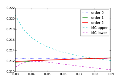
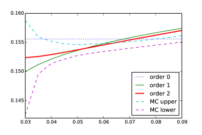
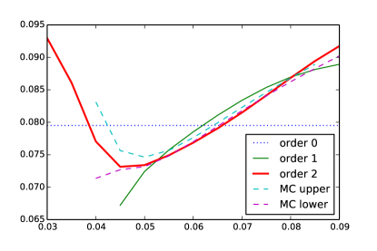
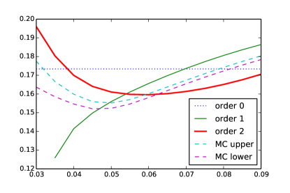
Figure 5.1. Implied volatilities of caplets with different strikes computed using the analytic approximation together with the Monte Carlo bound. Top graphs: Case 1 (left) and Case 2 (right). Bottom graphs: Case 3 (left) and Case 4 (right).

6. Acknowledgement

This research of Peter Tankov is partly supported by the Chair Financial Risks of the Risk Foundation sponsored by Société Générale.

References

• [\citeauthoryearBelomestny and SchoenmakersBelomestny and Schoenmakers2011] Belomestny, D. and J. Schoenmakers (2011). A jump-diffusion libor model and its robust calibration. Quantitative Finance 11(4), 529–546.
• [\citeauthoryearBenhamou, Gobet, and MiriBenhamou et al.2009] Benhamou, E., E. Gobet, and M. Miri (2009). Smart expansion and fast calibration for jump diffusions. Finance and Stochastics 13(4), 563–589.
• [\citeauthoryearBenhamou, Gobet, and MiriBenhamou et al.2010] Benhamou, E., E. Gobet, and M. Miri (2010). Time dependent heston model. SIAM Journal on Financial Mathematics 1(1), 289–325.
• [\citeauthoryearBrace, Ga̧tarek, and MusielaBrace et al.1997] Brace, A., D. Ga̧tarek, and M. Musiela (1997). The market model of interest rate dynamics. Mathematical Finance 7, 127–155.
• [\citeauthoryearCarr, Geman, Madan, and YorCarr et al.2007] Carr, P., H. Geman, D. B. Madan, and M. Yor (2007). Self-decomposability and option pricing. Mathematical Finance 17, 31–57.
• [\citeauthoryearČerný, Denkl, and KallsenČerný et al.2013] Černý, A., S. Denkl, and J. Kallsen (2013). Hedging in Lévy models and the time step equivalent of jumps. Preprint, arXiv:1309.7833.
• [\citeauthoryearDe FrancoDe Franco2012] De Franco, C. (2012). Two studies in risk management: portfolio insurance under risk measure constraint and quadratic hedge for jump processes. Ph. D. thesis, University Paris Diderot.
• [\citeauthoryearEberlein and KlugeEberlein and Kluge2007] Eberlein, E. and W. Kluge (2007). Calibration of Lévy term structure models. In M. Fu, R. A. Jarrow, J.-Y. Yen, and R. J. Elliott (Eds.), Advances in Mathematical Finance: In Honor of D. B. Madan, pp.  147–172. Birkhäuser.
• [\citeauthoryearEberlein and ÖzkanEberlein and Özkan2005] Eberlein, E. and F. Özkan (2005). The Lévy Libor model. Finance and Stochastics 9, 327–348.
• [\citeauthoryearJäckel and RebonatoJäckel and Rebonato2003] Jäckel, P. and R. Rebonato (2003). The link between caplet and swaption volatilities in a Brace-Gatarek-Musiela/Jamshidian framework: approximate solutions and empirical evidence. Journal of Computational Finance 6(4), 41–60.
• [\citeauthoryearKallsenKallsen2006] Kallsen, J. (2006). A didactic note on affine stochastic volatility models. In Y. Kabanov, R. Lipster, and J. Stoyanov (Eds.), From Stochastic Calculus to Mathematical Finance: The Shiryaev Festschrift, pp. 343–368. Springer.
• [\citeauthoryearKlugeKluge2005] Kluge, W. (2005). Time-Inhomogeneous Lévy Processes in Interest Rate and Credit Risk Models. Ph. D. thesis, University of Freiburg.
• [\citeauthoryearKohatsu-Higa and TankovKohatsu-Higa and Tankov2010] Kohatsu-Higa, A. and P. Tankov (2010). Jump-adapted discretization schemes for Lévy-driven sdes. Stochastic Processes and their Applications 120(11), 2258–2285.
• [\citeauthoryearMénassé and TankovMénassé and Tankov2015] Ménassé, C. and P. Tankov (2015). Asymptotic indifference pricing in exponential Lévy models. Preprint, arXiv:1502.03359.
• [\citeauthoryearMiltersen, Sandmann, and SondermannMiltersen et al.1997] Miltersen, K. R., K. Sandmann, and D. Sondermann (1997). Closed form solutions for term structure derivatives with log-normal interest rates. The Journal of Finance 52, 409–430.
• [\citeauthoryearPapapantoleon, Schoenmakers, and SkovmandPapapantoleon et al.2012] Papapantoleon, A., J. Schoenmakers, and D. Skovmand (2012). Efficient and accurate log-Lévy approximations to Lévy driven LIBOR models. Journal of Computational Finance 15(4), 3–44.
• [\citeauthoryearSandmann, Sondermann, and MiltersenSandmann et al.1995] Sandmann, K., D. Sondermann, and K. R. Miltersen (1995). Closed form term structure derivatives in a Heath–Jarrow–Morton model with log-normal annually compounded interest rates. In Proceedings of the Seventh Annual European Futures Research Symposium Bonn, pp.  145–165. Chicago Board of Trade.
• [\citeauthoryearSchoenmakersSchoenmakers2005] Schoenmakers, J. (2005). Robust Libor modelling and pricing of derivative products. CRC Press.