A numerical comparison of some
Multiscale Finite Element approaches for convection-dominated problems in heterogeneous media

Abstract

The purpose of this work is to investigate the behavior of Multiscale Finite Element type methods for advection-diffusion problems in the advection-dominated regime. We present, study and compare various options to address the issue of the simultaneous presence of both heterogeneity of scales and strong advection. Classical MsFEM methods are compared with adjusted MsFEM methods, stabilized versions of the methods, and a splitting method that treats the multiscale diffusion and the strong advection separately.

1 Introduction

We consider in this work an advection-diffusion equation that has both a multiscale character (encoded in an highly oscillatory diffusion coefficient) and a dominating advection. Formally, the equation reads as

$$-\text{div }(A^{\varepsilon}\nabla u^{\varepsilon})+b\cdot\nabla u^{\varepsilon}=f\quad\text{in }\Omega,\qquad u^{\varepsilon}=0\quad\text{on }\partial\Omega.$$ (1)

Our self-explanatory notation will be made precise in the sequel, along with the mathematical setting that allows to rigorously consider this equation. Our purpose is to investigate whether numerical methods dedicated to the treatment of multiscale phenomena, such as Multiscale Finite Element Methods (henceforth abbreviated as MsFEM) and methods specifically designed to address the dominating advection, such as Streamline-Upwind/Petrov-Galerkin (SUPG) type methods, can separately adequately address the twofold problem, or, if need be, to discover how these methods may be combined to form the best possible approach in various regimes.

Equation (1) is practically relevant and interesting per se. Our study of this particular equation is nevertheless rather to be seen as a step toward the study of the following much more relevant case, which will be performed in an upcoming work [23]: an (single-scale) advection-diffusion equation, with a dominating advection term, posed on a perforated domain (in that vein, see [8]). In a previous, somewhat related couple of studies [21, 22], we have used with much benefit the highly oscillatory case as a test-bed for designing and studying approaches subsequently used for the more challenging perforated case.

Methods of the MsFEM type have proved efficient in a number of contexts. In essence, they are based upon choosing, as specific finite dimensional basis to expand the numerical solution upon, a set of functions that themselves are solutions to a highly oscillatory local problem, at scale $\varepsilon$, involving the differential operator present in the original equation. This problem-dependent basis set is likely to better encode the fine-scale oscillations of the solution and therefore allow to capture the solution more accurately. Numerical observation along with mathematical arguments prove that this is indeed generically the case. For the specific advection-diffusion equation (1) we consider here, two natural options for the construction of the basis set are (i) to pick as basis functions solutions to the (multiscale) diffusion operator only, or (ii) to also involve in the definition of the functions the advection operator. These two approaches will be among the set of approaches considered and tested below. In the former option, when the basis functions do not involve the advection operator, one may fear that, in the presence of advection, and especially in the presence of a strong advection that dominates the diffusion – a regime we focus on throughout this work –, the accuracy of the classical MsFEM dramatically deteriorates. This is for instance the case, "when $\varepsilon=1$", for classical $\mathbb{P}^{1}$ finite element methods. Stabilization procedures are then in order and we will indeed adapt such a procedure to the present multiscale context. On the other hand, in the latter option, it is unclear whether the presence of the advection term also for the definition of the basis functions allows, or not, for the method to also perform well in the advection-dominated regime. This will be investigated below. However well such an approach performs, the fact that the advection is involved in the definition of the finite elements might create issues, and be prohibitively expensive computationally, when the advection varies and the equation needs to be solved repeatedly, either because the present steady state setting of (1) is in fact a time iteration within the numerical simulation of a time-dependent equation, or because equation (1) is part of an optimization, or inverse problem. Also, inserting the advection term in the definition of the basis functions is a very invasive implementation, which might be problematic in some contexts. Both observations are sufficient motivations to also consider a splitting method, separately addressing the multiscale character with a classical MsFEM approach for the solution of the diffusion operator, and solving a single-scale advection-dominated advection-diffusion equation with a stabilized $\mathbb{P}^{1}$ method.

The four MsFEM-type approaches we have just mentioned (classical – that is, with basis functions constructed from diffusion only –, classical and stabilized, advection-diffusion based, splitting the advection and the multiscale character) will be studied and compared. For reference, we will also use a $\mathbb{P}^{1}$ finite element method, stabilized or not, in particular to investigate when the multiscale nature of the problem and the domination of the convection matter, or not.

In the context of HMM-type methods, multiscale advection-diffusion problems with dominating convection have been considered e.g. in [1].

Our article is organized as follows. Section 2 briefly recalls, essentially for the sake of self-consistency, some basic, classical and well-known facts on the building blocks (stabilization, multiscale approaches) we use, and describes in more details the numerical approaches we consider. We next provide, in Section 3, a complete numerical analysis of the approaches in the one-dimensional setting. We are unfortunately unable to conduct the same analysis in higher dimensions, but some of the issues we raise and discuss in the one-dimensional context are definitely useful to understand the approaches in a more general context. In particular, we point out that the direct application of an SUPG stabilization on MsFEM leads to an approach that is not strongly consistent (in sharp contrast to its single-scale, say $\mathbb{P}^{1}$ version), because the basis functions are not known analytically but only up to the numerical error present in the offline precomputation. We provide a solution to that difficulty. We show that, in spite of a lack of consistency, the method we design can be certified (and numerical observation will later show it performs efficiently). We also devote some time to the detailed study, in any dimension, of the convergence of the splitting approach.

Our final Section 4 presents a comprehensive series of numerical tests and comparisons. An executive summary of our main conclusions is as follows:

• (i) the best possible approach among all those we consider is the stabilized version of MsFEM, unless one does not want to be intrusive in which case the splitting approach performs approximately equally well, for an online computational cost that might be significantly larger, especially for problems of large size for which iterative solvers have to employed;

• (ii) the method using basis functions built upon the full advection-diffusion operator is not sufficiently stable to perform well in the advection-dominated regime;

• (iii) when advection outrageously dominates diffusion, the multiscale character of the solution (at least in the bulk of the domain) is essentially overshadowed by the convection, and a “classical” stabilized $\mathbb{P}^{1}$ finite element method performs as well as a MsFEM-type approach, a somewhat intuitive fact that our study allows to confirm.

Further details on the approaches considered are given in the body of the text.

2 Description of the numerical approaches

We describe in Section 2.1 the standard numerical tools we use throughout this work. We next present in Section 2.2 the four numerical methods we study.

2.1 Building blocks

In this section, we briefly recall for convenience some classical elements on the two building blocks we make use of to construct the approaches we study, namely stabilization methods (more specifically, SUPG type methods) and Multiscale Finite Element Methods (MsFEM). The reader already familiar with these notions may easily skip the present section and directly proceed to Section 2.2.

2.1.1 Stabilized methods

We temporarily consider the single-scale advection-diffusion problem

$$-\alpha\Delta u+b\cdot\nabla u=f\quad\text{in }\Omega,\qquad u=0\quad\text{on }\partial\Omega,$$ (2)

where $\Omega$ is a smooth bounded domain of $\mathbb{R}^{d}$, $\alpha>0$, $b\in(L^{\infty}(\Omega))^{d}$ and $f\in L^{2}(\Omega)$. We suppose that

$$\text{div }b=0\quad\text{in }\Omega,$$ (3)

so that problem (2) is coercive and amenable to standard numerical analysis techniques for coercive problems. We shall discuss the case of non-coercive problems in Remark 1 below.

Let $\mathcal{T}_{H}$ be a uniform regular mesh of size $H$ discretizing $\Omega$, and let $V_{H}$ be the classical $\mathbb{P}^{1}$ Finite Element space associated to this mesh. The classical Galerkin approximation of (2) reads as the following variational formulation:

$$\text{Find }u_{H}\in V_{H}\text{ such that, for any $v_{H}\in V_{H}$,}\quad a(u_{H},v_{H})=F(v_{H}),$$

where

$$a(u,v)=\int_{\Omega}\alpha\nabla u\cdot\nabla v+(b\cdot\nabla u)v,\qquad F(v)=\int_{\Omega}fv.$$ (4)

Since the solution $u$ to (2) is in $H^{2}(\Omega)$, we have the following error estimate as a direct consequence of Céa’s lemma:

$$\|u-u_{H}\|_{H^{1}(\Omega)}\leq CH(1+\text{Pe}\,H)\,\|u\|_{H^{2}(\Omega)},$$ (5)

where $C$ is independent of $H$ and $b$. We have introduced, as is classical, the global Péclet number

$$\text{Pe}=\frac{\|b\|_{L^{\infty}(\Omega)}}{2\alpha}$$ (6)

of problem (2). We thus see that the larger the product Pe$\,H$, the larger the potential numerical error. Intuitively, the problem becomes less and less coercive as advection increasingly dominates over diffusion and, eventually, the coercivity is lost [11, Section 3.5.2] when Pe goes to $+\infty$. As is well-known, the Péclet number directly affects the quality of the numerical results. With the standard $\mathbb{P}^{1}$ finite element approximation, oscillations polluting the solution are observed (see Figure 1 below).

Stabilization is a classical subject of numerical analysis. Many works (see e.g. [17] and the textbooks [28, 29]) have been devoted to designing stabilized methods for the convection-dominated regime. They consist in considering the following problem:

$$\text{Find }u_{H}^{s}\in V_{H}\text{ such that, for any $v_{H}\in V_{H}$,}$$

$$a(u_{H}^{s},v_{H})+a_{\text{stab}}(u_{H}^{s},v_{H})=F(v_{H})+F_{\text{stab}}(v_{H}),$$ (7)

where $a$ and $F$ are defined by (4) and $a_{\text{stab}}$ and $F_{\text{stab}}$ are defined by

$$a_{\text{stab}}(u_{H}^{s},v_{H})=\sum_{\mathbf{K}\in\mathcal{T}_{H}}\bigg{(}\tau_{\mathbf{K}}\mathcal{L}u_{H}^{s},(\mathcal{L}_{ss}+\rho\mathcal{L}_{s})v_{H}\bigg{)}_{\mathbf{K}},$$ (8)

$$F_{\text{stab}}(v_{H})=\sum_{\mathbf{K}\in\mathcal{T}_{H}}\bigg{(}\tau_{\mathbf{K}}f,(\mathcal{L}_{ss}+\rho\mathcal{L}_{s})v_{H}\bigg{)}_{\mathbf{K}},$$ (9)

where, for any $u$ and $v$, $\displaystyle(u,v)_{\mathbf{K}}=\int_{\mathbf{K}}u\,v$, $\mathcal{L}_{s}u=-\alpha\Delta u$ and $\mathcal{L}_{ss}u=b\cdot\nabla u$ are the symmetric part and the skew-symmetric part of the advection-diffusion operator ${\cal L}v=-\alpha\Delta v+b\cdot\nabla v$, respectively (recall that $b$ is divergence free in view of (3)). The stabilization parameter $\tau_{\mathbf{K}}$ is chosen, roughly, of the order of $\displaystyle\frac{H}{\|b\|_{L^{\infty}(\Omega)}}$. The choice of $\rho$ leads to different stabilized methods: (i) the Douglas-Wang method (DW) when $\rho=-1$, the Streamline Upwind Petrov-Galerkin method (SUPG) when $\rho=0$ and the Galerkin Least Square method (GLS) when $\rho=1$. The three stabilized methods, applied on problem (2), coincide when $V_{H}$ is the $\mathbb{P}^{1}$ Finite Element space associated to the mesh $\mathcal{T}_{H}$.

The modification of the discrete bilinear form as in (7) allows to obtain the estimate

$$\|u-u_{H}^{s}\|_{H^{1}(\Omega)}\leq CH\left(1+\sqrt{\text{Pe}\,H}\right)\|u\|_{H^{2}(\Omega)},$$ (10)

where again $C$ is independent of $H$ and $b$. For large Péclet numbers (that is, Pe$\,H>1$), this estimate is better than (5). More accurate numerical results are indeed obtained: see Figure 1 below. Note also that, in the right-hand sides of (5) and (10), $\|u\|_{H^{2}(\Omega)}$ depends on $b$, a fact that we will recall in Remark 11 below.

Estimate (10) is typically obtained under the assumptions

$$\frac{|b(x)|}{2\alpha}H\geq 1\quad\text{for almost all $x\in\Omega$},$$ (11)

and for the stabilization parameter

$$\tau_{\mathbf{K}}(x)=\frac{H}{2|b(x)|}\quad\text{for all }\mathbf{K}\in\mathcal{T}_{H}.$$ (12)

For the sake of completeness, and also because we will use similar arguments in Section 3 below for the multiscale setting, we provide the proof of (10) in Appendix A below.

Remark 1.

Notice that all the above analysis assumes that problem (2) is coercive (see (3)). This is usually the case in the literature, see [6, 29]. To the best of our knowledge, the analysis of the stabilized methods of the type (7) has not been performed in the non-coercive case. A stabilized numerical method designed for nonsymmetric noncoercive problems is proposed and studied in [7]. The method requires to solve the original problem coupled with an adjoint problem using stabilized finite element methods. Error estimates in $H^{1}$ and $L^{2}$ norms are proved under the assumption of well-posedness of the problem. Least-square methods for noncoercive elliptic problems have also been studied, see e.g. [4, 20].

Remark 2.

The stabilized methods (7) can also be understood in the framework of the Variational Multiscale Methods [17].

Remark 3.

The choice of an optimal stabilization parameter $\tau_{\mathbf{K}}$ is a difficult and sensitive question, since it affects the quality of the numerical approximation. We refer e.g. to [5, 12, 26]. The Variational Multiscale Methods [17] give an interpretation of the stabilization parameter. If we assume $\tau_{\mathbf{K}}$ to be constant on each mesh element $\mathbf{K}$, the Variational Multiscale Methods yield the formula

$$\tau_{\mathbf{K}}=\frac{1}{|\mathbf{K}|}\int_{\mathbf{K}}\int_{\mathbf{K}}g_{\mathbf{K}},$$ (13)

where $g_{\mathbf{K}}$ is the Green’s function of the operator ${\cal L}^{\star}$ (i.e. the adjoint of ${\cal L}$) with homogeneous Dirichlet boundary conditions on $\partial\mathbf{K}$. Simplifying assumptions are next used to infer, from (13), a practical expression for $\tau_{\mathbf{K}}$.

For the sake of illustration, and because it allows us to introduce notions useful for what follows, we briefly consider the one-dimensional example

$$-\alpha u^{\prime\prime}+bu^{\prime}=f\quad\text{in }(0,1),\qquad u(0)=u(1)=0,$$ (14)

for a constant $b$. In that case, the expression (13) can be analytically computed and yields the choice

$$\tau_{\mathbf{K}}=\frac{H}{2|b|}\left(\coth(\text{Pe}\,H)-\frac{1}{\text{Pe}\,H}\right).$$ (15)

On Figure 1, we show the exact solution to (14) as well as two numerical approximations. We set $\alpha=1/256$, $b=1$, $f=1$ and $H=1/16$, so that we are in the convection-dominated regime. Table 1 shows the relative errors of the methods.

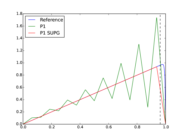
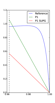
Figure 1: Exact and numerical solutions to (14) for Pe$\,H=8$. Left: Plot on the whole domain. Right: Close-up on the boundary layer. The vertical dashed line delineates the boundary layer.

	$L^{2}$: $\mathbb{P}^{1}$	$L^{2}:$ $\mathbb{P}^{1}$ SUPG	$H^{1}$: $\mathbb{P}^{1}$	$H^{1}$: $\mathbb{P}^{1}$ SUPG
Outside the layer	0.3217	0.0624	0.8913	0.2228
Inside the layer	0.0297	0.1549	0.3722	0.7163
In the whole domain	0.3513	0.2173	1.2635	0.9391

Table 1: Relative errors for (14) with $\alpha=1/256$, $b=1$, $f=1$ and $H=1/16$. The parameter $\tau_{\mathbf{K}}$ is given by (15).

On Figure 1, we can distinguish two regions. Outside the boundary layer, the $\mathbb{P}^{1}$ SUPG method accurately approximates the solution. It has no spurious oscillations, in contrast to the standard $\mathbb{P}^{1}$ method. Inside the boundary layer, the $\mathbb{P}^{1}$ SUPG method only poorly performs.

2.1.2 MsFEM approaches

We now insert a multiscale character in our problem and temporarily erase the transport field $b$, which we will shortly reinstate in the next section. We consider the solution $u^{\varepsilon}\in H^{1}_{0}(\Omega)$ to

$$-\text{div }(A^{\varepsilon}\nabla u^{\varepsilon})=f\quad\text{in }\Omega,\qquad u^{\varepsilon}=0\quad\text{on }\partial\Omega.$$ (16)

We assume that the diffusion matrix $A^{\varepsilon}$, encoding the oscillations at the small scale, is elliptic in the sense that there exists $0<\alpha_{1}\leq\alpha_{2}$ such that

$$\forall\varepsilon,\quad\forall\xi\in\mathbb{R}^{d},\quad\alpha_{1}|\xi|^{2}\leq(A^{\varepsilon}(x)\xi)\cdot\xi\leq\alpha_{2}|\xi|^{2}\quad\text{a.e. on }\Omega.$$ (17)

Throughout this article, we shall perform our theoretical analysis for general, not necessarily symmetric, matrix-valued coefficients $A^{\varepsilon}$, not necessarily either of the form $\displaystyle A^{\varepsilon}=A\left(\cdot/\varepsilon\right)$ for a fixed matrix $A$ (although one may consider such a case to fix the ideas). In our numerical tests, however, we only consider a scalar coefficient $A^{\varepsilon}$.

The bottom line of the MsFEM is to perform a Galerkin approximation using specific basis functions, which are precomputed (in an offline stage) and adapted to the problem considered.

On the prototypical multiscale diffusion problem (16), the method, in one of its simplest variant, consists of the following three steps:

1. Introduce a discretization of $\Omega$ with a coarse mesh; throughout this article, we work with the $\mathbb{P}^{1}$ Finite Element space

   $$V_{H}=\text{Span}\left\{\phi^{0}_{i},1\leq i\leq N_{V_{H}}\right\}\subset H^{1}_{0}(\Omega);$$ (18)

2. Solve the local problems (one for each basis function for the coarse mesh)

   $$-\text{div }\left(A^{\varepsilon}\nabla\psi_{i}^{\varepsilon,\mathbf{K}}\right)=0\quad\text{in }\mathbf{K},\qquad\psi^{\varepsilon,\mathbf{K}}_{i}=\phi^{0}_{i}\quad\text{on }\partial\mathbf{K},$$ (19)

   on each element $\mathbf{K}$ of the coarse mesh, in order to build the multiscale basis functions.

3. Apply a standard Galerkin approximation of (16) on the space

   $$V_{H}^{\varepsilon}=\text{Span}\left\{\psi^{\varepsilon}_{i},\ 1\leq i\leq N_{V_{H}}\right\}\subset H^{1}_{0}(\Omega),$$ (20)

   where $\psi^{\varepsilon}_{i}$ is such that $\left.\psi^{\varepsilon}_{i}\right|_{\mathbf{\mathbf{K}}}=\psi^{\varepsilon,\mathbf{K}}_{i}$ for all $\mathbf{K}\in\mathcal{T}_{H}$.

The error analysis of the MsFEM method in the above case (16), for $\displaystyle A^{\varepsilon}=A_{\rm per}\left(\cdot/\varepsilon\right)$ with $A_{\rm per}$ a fixed periodic matrix, has been performed in [15] (see also [9, Theorem 6.5]). The main result is stated in the following Theorem.

Theorem 4.

We consider the periodic case $\displaystyle A^{\varepsilon}(x)=A_{\rm per}\left(x/\varepsilon\right)$. We assume that $A_{\rm per}$ is Hölder continuous, that the solution $u^{\star}$ to the homogenized problem associated to (16) belongs to $W^{2,\infty}(\Omega)$ and that $H>\varepsilon$. Let $u^{\varepsilon}_{H}$ be the MsFEM approximation of the solution $u^{\varepsilon}$ to (16). Then

$$\|u^{\varepsilon}-u^{\varepsilon}_{H}\|_{H^{1}(\Omega)}\leq C\left(H+\sqrt{\varepsilon}+\sqrt{\frac{\varepsilon}{H}}\right),$$ (21)

where $C$ is a constant independent of $H$ and $\varepsilon$.

When the coarse mesh size $H$ is close to the scale $\varepsilon$, a resonance phenomenon, encoded in the term $\sqrt{\varepsilon/H}$ in (21), occurs and deteriorates the numerical solution. The oversampling method [16] is a popular technique to reduce this effect. In short, the approach, which is non-conforming, consists in setting each local problem on a domain slightly larger than the actual element considered, so as to become less sensitive to the arbitrary choice of boundary conditions on that larger domain, and next truncate on the element the functions obtained. That approach allows to significantly improve the results compared to using linear boundary conditions as in (19). In the periodic case, we have the following estimate (see [10]).

Theorem 5.

Assume the setting and the notation of Theorem 4. Assume additionally that the distance between an element $\mathbf{K}$ and the boundary of the macro element used in the oversampling is larger than $H$. Then

$$\|u^{\varepsilon}-u^{\varepsilon}_{H}\|_{H^{1}(\mathcal{T}_{H})}\leq C\left(H+\sqrt{\varepsilon}+\frac{\varepsilon}{H}\right),$$

where $\displaystyle\|u^{\varepsilon}-u^{\varepsilon}_{H}\|_{H^{1}(\mathcal{T}_{H})}=\sqrt{\sum_{\mathbf{K}\in\mathcal{T}_{H}}\|u^{\varepsilon}-u^{\varepsilon}_{H}\|^{2}_{H^{1}(\mathbf{K})}}$ is the $H^{1}$ broken norm of $u^{\varepsilon}-u^{\varepsilon}_{H}$.

Remark 6.

The boundary conditions imposed in (19) are the so-called linear boundary conditions. Besides the linear boundary conditions, and the oversampling technique alluded to above, there are many other possible boundary conditions for the local problems. They may give rise to conforming, or non-conforming approximations. The choice sensitively affects the overall accuracy. We will explore this issue, in our specific context, in Section 4.2.5 below.

It is important to notice that the estimates of Theorems 4 and 5 hold true assuming that the multiscale basis functions employed to compute the approximation $u^{\varepsilon}_{H}$ are the exact solutions of the local problems. In practice of course, the local problems (19) are only approximated numerically, using a fine mesh of size $h$ sufficiently small to capture the oscillations at scale $\varepsilon$.

As mentioned above, our purpose is to understand how to adapt the stabilization methods and the MsFEM methods in order to efficiently approximate

$$-\text{div }(A^{\varepsilon}\nabla u^{\varepsilon})+b\cdot\nabla u^{\varepsilon}=f\quad\text{in }\Omega,\qquad u^{\varepsilon}=0\quad\text{on }\partial\Omega,$$ (22)

where $A^{\varepsilon}\in(L^{\infty}(\Omega))^{d\times d}$ satisfies (17), $b\in(L^{\infty}(\Omega))^{d}$ and $f\in L^{2}(\Omega)$. Notice that the transport field $b$ is assumed to be independent of $\varepsilon$. We also choose it divergence-free as in (3). The variational formulation of (22) is:

$$\text{Find }u^{\varepsilon}\in H^{1}_{0}(\Omega)\text{ such that, for any $v\in H^{1}_{0}(\Omega)$,}\quad a^{\varepsilon}(u^{\varepsilon},v)=F(v),$$ (23)

where

$$a^{\varepsilon}(u,v)=\int_{\Omega}(A^{\varepsilon}\nabla u)\cdot\nabla v+(b\cdot\nabla u)\,v,\qquad F(v)=\int_{\Omega}fv.$$ (24)

We now introduce in Section 2.2 below the four numerical approaches we consider.

2.2 Our four numerical approaches

2.2.1 The classical MsFEM and its stabilized version

The classical MsFEM described in Section 2.1.2 is the first approach we consider. It performs a Galerkin approximation of (22) on the space (19)-(20). Notice that in this approximation, the transport term $b\cdot\nabla$, although present in the equation (22), is absent from the local problems (19) and thus from the definition of the basis functions. It is immediate to realize that this approach coincides with the standard $\mathbb{P}^{1}$ method on (2) when $A^{\varepsilon}=\alpha\,\text{Id}$. Consequently, the method is expected to be unstable in the convection-dominated regime, as recalled in Section 2.1.1, and this is indeed observed in practice, as will be seen in Section 4.2.3.

This motivates the introduction of a stabilized version of this method, which is the adaptation to the multiscale context of the classical SUPG method. As we shall now see, some difficulty arises regarding the consistency of the approach, owing to the fact that the basis functions we use in practice are only approximate.

First, we consider the exact approximation space $V_{H}^{\varepsilon}$ defined by (20). The SUPG stabilization, readily applied to our problem (23), yields the following variational formulation:

$$\text{Find }u^{\varepsilon}_{H}\in V_{H}^{\varepsilon}\text{ such that, for any $v_{H}^{\varepsilon}\in V_{H}^{\varepsilon}$,}$$

$$a^{\varepsilon}(u^{\varepsilon}_{H},v^{\varepsilon}_{H})+a_{\text{stab}}(u^{\varepsilon}_{H},v^{\varepsilon}_{H})=F(v_{H}^{\varepsilon})+F_{\text{stab}}(v_{H}^{\varepsilon}),$$ (25)

where we recall that the SUPG stabilization terms are (see (8) and (9))

$$a_{\text{stab}}(u_{H}^{\varepsilon},v_{H}^{\varepsilon}) =\sum_{\textbf{K}\in\mathcal{T}_{H}}\Big{(}\tau_{\mathbf{K}}\left(-\text{div }\left(A^{\varepsilon}\nabla u_{H}^{\varepsilon}\right)+b\cdot\nabla u_{H}^{\varepsilon}\right),b\cdot\nabla v_{H}^{\varepsilon}\Big{)}_{L^{2}(\mathbf{K})},$$ (26)

$$F_{\text{stab}}(v_{H}^{\varepsilon}) =\sum_{\mathbf{K}\in\mathcal{T}_{H}}\bigg{(}\tau_{\mathbf{K}}f,b\cdot\nabla v_{H}^{\varepsilon}\bigg{)}_{\mathbf{K}}.$$

The method is, as is well known, strongly consistent. Because of the definition of the approximation space $V_{H}^{\varepsilon}$, we have

$$a_{\text{stab}}(u_{H}^{\varepsilon},v_{H}^{\varepsilon})=a_{\text{upw}}(u_{H}^{\varepsilon},v_{H}^{\varepsilon})\quad\text{for any }(u_{H}^{\varepsilon},v_{H}^{\varepsilon})\in(V_{H}^{\varepsilon})^{2},$$ (27)

where

$$a_{\text{upw}}(u_{H}^{\varepsilon},v_{H}^{\varepsilon})=\sum_{\textbf{K}\in\mathcal{T}_{H}}\left(\tau_{\mathbf{K}}b\cdot\nabla u_{H}^{\varepsilon},b\cdot\nabla v_{H}^{\varepsilon}\right)_{L^{2}(\mathbf{K})}.$$ (28)

In practice however, we only know a discrete approximation $\psi^{\varepsilon,h}$, on a fine mesh $\mathbf{K}_{h}$, of the solution $\psi^{\varepsilon}$ to (19). Put differently, we manipulate $V^{\varepsilon}_{H,h}=\text{Span}\{\psi^{\varepsilon,h}_{i},1\leq i\leq N_{V_{H}}\}$ instead of $V_{H}^{\varepsilon}$. It follows that, for example when $A^{\varepsilon}\in\mathcal{C}^{0}(\overline{\Omega})$ and we use a $\mathbb{P}^{1}$ approximation on a fine mesh $\mathbf{K}_{h}$ for the local problem (19), $A^{\varepsilon}\nabla u_{H,h}^{\varepsilon}$ may be discontinuous at the edges of the mesh $\mathbf{K}_{h}$, and $-\text{div }(A^{\varepsilon}\nabla u_{H,h}^{\varepsilon})\notin L^{1}_{\rm loc}(\mathbf{K})$.

We may consider at least two ways to circumvent that difficulty. First, if the matrix coefficient $A^{\varepsilon}$ is locally sufficiently regular, we may define the stabilization term as

$$\widetilde{a}_{\text{stab}}(u_{H,h}^{\varepsilon},v_{H,h}^{\varepsilon})\\ =\sum_{\mathbf{K}\in\mathcal{T}_{H}}\sum_{\kappa\subset K_{h}}\Big{(}\tau_{\mathbf{K}}\left(-\text{div }\left(A^{\varepsilon}\nabla u_{H,h}^{\varepsilon}\right)+b\cdot\nabla u_{H,h}^{\varepsilon}\right),b\cdot\nabla v_{H,h}^{\varepsilon}\Big{)}_{L^{2}(\mathbf{\kappa})}.$$

When, as is the case here, we employ a $\mathbb{P}^{1}$ approximation on $\mathbf{K}_{h}$, all we need for this stabilization term to make sense is that the vector field $\text{div}\left(A^{\varepsilon}\right)$ belongs to $L^{1}(\kappa)$ for all $\kappa\subset K_{h}$. This is more demanding than the simple classical assumption $A^{\varepsilon}\in L^{\infty}(\Omega)$. Under this assumption, we obtain a strongly consistent stabilized method. We will however not proceed in this direction and favor an alternate approach, to which we now turn.

Based upon the observation (27) for the "ideal" space $V_{H}^{\varepsilon}$, we may use the stabilization term (28) rather than (26). In contrast to (26), the quantity (28) is also well defined on $V^{\varepsilon}_{H,h}$. And this holds true without any additional regularity assumption on $A^{\varepsilon}$. The Stab-MsFEM method we employ is hence defined by the following variational formulation:

$$\text{Find }u^{\varepsilon}_{H,h}\in V^{\varepsilon}_{H,h}\text{ such that, for any $v_{H,h}^{\varepsilon}\in V^{\varepsilon}_{H,h}$,}$$

$$a^{\varepsilon}(u^{\varepsilon}_{H,h},v^{\varepsilon}_{H,h})+a_{\text{upw}}(u^{\varepsilon}_{H,h},v^{\varepsilon}_{H,h})=F(v_{H,h}^{\varepsilon})+F_{\text{stab}}(v_{H,h}^{\varepsilon}).$$ (29)

We emphasize that employing that stabilization comes at a price: we give up on strong consistency. We provide in Section 3.2, Theorem 49 below, an error estimate in the one-dimensional setting for this method. Despite the absence of consistency, we can still prove that the method is convergent.

2.2.2 The Adv-MsFEM variant

In contrast to our first two approaches, the Adv-MsFEM approach we discuss in this section accounts for the transport field in the local problems. For each mesh element $\mathbf{K}\in\mathcal{T}_{H}$, we indeed now consider

$$-\text{div }\left(A^{\varepsilon}\nabla\phi^{\varepsilon,\mathbf{K}}_{i}\right)+b\cdot\nabla\phi^{\varepsilon,\mathbf{K}}_{i}=0\ \ \text{ in $\mathbf{K}$},\qquad\phi^{\varepsilon,\mathbf{K}}_{i}=\phi^{0}_{i}\ \ \text{ on $\partial\mathbf{K}$},$$ (30)

instead of (19), and next the approximation space

$$V_{H}^{\varepsilon,Adv}=\text{Span}\left\{\phi^{\varepsilon}_{i},\ 1\leq i\leq N_{V_{H}}\right\}\subset H^{1}_{0}(\Omega)$$

defined as in (20). Problem (30) is an advection-diffusion problem with, in principle, a high Péclet number. Nevertheless, the problem is local and is to be solved offline, so we may easily employ a mesh size sufficiently fine to avoid the issues presented in Section 2.1.1.

There is however a difficulty in considering (30) and $b$-dependent basis functions $\phi^{\varepsilon,\mathbf{K}}_{i}$. In the context where we want to repeatedly solve (22) for multiple $b$, for instance when $b$ depends on an external parameter such as time, the method becomes prohibitively expensive as we will see in Section 4.3.

We note in passing the following consistency. In the one-dimensional single-scale example (14), the stiffness matrix of the Adv-MsFEM method is

$$M_{\text{Adv-MsFEM}}=\text{Tridiag}\left(\frac{-b\exp\left(bH/\alpha\right)}{\exp\left(bH/\alpha\right)-1},|b|\coth\left(\frac{|b|H}{2\alpha}\right),\frac{-b}{\exp\left(bH/\alpha\right)-1}\right).$$

It then coincides with the stiffness matrix $M_{\mathbb{P}^{1}\text{SUPG}}$ of the $\mathbb{P}^{1}$ SUPG method with $\tau_{\mathbf{K}}$ given by (15).

We also note that, in view of (26)–(30), we have that $a_{\text{stab}}(u_{H}^{\varepsilon,\text{Adv}},v_{H}^{\varepsilon,\text{Adv}})=0$ for any $(u_{H}^{\varepsilon,\text{Adv}},v_{H}^{\varepsilon,\text{Adv}})\in(V_{H}^{\varepsilon,Adv})^{2}$. Such a stabilization is therefore void on the Adv-MsFEM method. Actually, we shall see in the numerical tests of Section 4.2 that the Adv-MsFEM method is only moderately sensitive to the Péclet number.

MsFEM type basis functions depending on the transport term for multiscale advection-diffusion problems have already considered in the literature. In [25], two settings are investigated. The Adv-MsFEM is first applied to the time-dependent multiscale advection-diffusion equation

$$\partial_{t}u^{\varepsilon}-\Delta u_{\varepsilon}+\frac{1}{\varepsilon}b\left(\frac{\cdot}{\varepsilon}\right)\cdot\nabla u^{\varepsilon}=0\quad\text{ in }\mathbb{R}^{2},$$

with $b=\nabla^{\perp}\psi$ where $\displaystyle\psi\left(x\right)=\psi\left(x_{1},x_{2}\right)=\frac{1}{4\pi^{2}}\sin({2\pi x_{1}})\sin({2\pi x_{2}})$. The field $b$ is thus $\mathbb{Z}^{d}$-periodic, divergence-free and of mean zero. The purpose is then to only capture macroscopic properties of the solution $u^{\varepsilon}$. Also in [25], the Adv-MsFEM is investigated on the problem

$$-\Delta u^{\varepsilon}+b^{\varepsilon}\cdot\nabla u^{\varepsilon}=f,$$

with $b^{\varepsilon}\in(L^{\infty}(\Omega))^{2}$ and $f\in L^{2}(\Omega)$. Only the following $L^{2}$ error estimate

$$\frac{\|u^{\varepsilon}-u^{\varepsilon}_{H}\|_{L^{2}(\Omega)}}{\|u^{\varepsilon}\|_{L^{2}(\Omega)}}\leq C\frac{\varepsilon}{H}+CH^{2}\|f\|_{L^{2}(\Omega)}$$

is derived, and not an $H^{1}$ estimate which would be sensitive to how well the fine oscillations are captured by the numerical approach. It is completed in the periodic case, where $\displaystyle b^{\varepsilon}(x)=\frac{1}{\varepsilon}b_{\rm per}\left(\frac{x}{\varepsilon}\right)$ for a fixed, periodic, divergence-free function $b_{\rm per}$ of mean zero, under some assumptions which have been numerically verified on some examples. An experimental study of convergence is performed and shows good agreement with the above theoretical error estimate.

A second reference we wish to cite is [24]. The author studies there the problem

$$\left\{\begin{aligned} &\rho^{\varepsilon}\partial_{t}u^{\varepsilon}-\text{div}(A^{\varepsilon}\nabla u^{\varepsilon})+\frac{1}{\varepsilon}b^{\varepsilon}\cdot\nabla u^{\varepsilon}=0\quad\text{ in }(0,1)^{d}\times(0,T),\\ &u^{\varepsilon}(0,\cdot)=u^{0}\quad\text{ in }(0,1)^{d},\\ &u^{\varepsilon}(t,\cdot)\text{ is }(0,1)^{d}\text{-periodic,}\end{aligned}\right.$$

where $u^{0}\in W^{m,\infty}_{\rm per}((0,1)^{d})$ with $m\geq 3$. The functions $\rho^{\varepsilon}\in L^{\infty}((0,1)^{d})$, $b^{\varepsilon}\in(L^{\infty}((0,1)^{d}))^{d}$ and $A^{\varepsilon}\in(L^{\infty}((0,1)^{d}))^{d\times d}$ do not depend on time. It is assumed that there exists a constant $\rho_{m}>0$ such that $\rho^{\varepsilon}\geq\rho_{m}$ a.e. on $(0,1)^{d}$, and that $b^{\varepsilon}$ is divergence-free. In contrast to [25], the mean of $b^{\varepsilon}$ is not assumed to vanish (but periodic boundary conditions are imposed on $\partial(0,1)^{d}$). In the convection-dominated regime, the problem is stabilized using the characteristics method for integrating the transport operator $\displaystyle\partial_{t}+\frac{b^{\star}_{H}}{\varepsilon}\cdot\nabla$, and the multiscale finite element method for the remaining part of the convection term, i.e. $\displaystyle\frac{b^{\varepsilon}-\rho^{\varepsilon}b^{\star}_{H}}{\varepsilon}\cdot\nabla$, where $\displaystyle b^{\star}_{H}|_{\mathbf{K}}=\frac{\int_{\mathbf{K}}b^{\varepsilon}}{\int_{\mathbf{K}}\rho^{\varepsilon}}$ for all $\mathbf{K}\in\mathcal{T}_{H}$. The MsFEM approach which is used in [24] is inspired by the variant of the Multiscale Finite Element approach introduced in [2] for purely diffusive problems. The multiscale basis functions are thus defined by $\phi^{\varepsilon}_{j}(x)=\phi^{0}_{j}\Big{(}w^{\varepsilon,H}(x)\Big{)}$ for $1\leq j\leq N_{V_{H}}$, where $\phi^{0}_{j}$ are the $\mathbb{P}^{1}$ basis functions and $w^{\varepsilon,H}|_{\mathbf{K}}=(w^{\varepsilon,\mathbf{K}}_{1},\dots,w^{\varepsilon,\mathbf{K}}_{d})$ for each $\mathbf{K}\in\mathcal{T}_{H}$, where, for any $i=1,\dots,d$, the function $w^{\varepsilon,\mathbf{K}}_{i}$ is the solution to

$$-\text{div }\left(A^{\varepsilon}\nabla w^{\varepsilon,\mathbf{K}}_{i}\right)+\frac{b^{\varepsilon}-\rho^{\varepsilon}b^{\star}_{H}}{\varepsilon}\cdot\nabla w^{\varepsilon,\mathbf{K}}_{i}=0\ \ \text{ in $\mathbf{K}$},\qquad w^{\varepsilon,\mathbf{K}}_{i}=x_{i}\ \ \text{ on $\partial\mathbf{K}$}.$$

Note that, as in (30), the basis functions depend on the convection field. An error estimate is established in [24] for the periodic case.

2.2.3 A splitting approach

The fourth, and last approach we consider is a splitting method that decomposes (22) into a single-scale, convection-dominated problem and a multiscale, purely diffusive problem. The main motivation for considering such a splitting approach is the non-intrusive character of the approach. In practice, one may couple legacy codes that are already optimized for each of the two subproblems.

Of course, splitting methods have been used in a large number of contexts. To cite only a couple of works relevant to our context, we mention [19] for a review on the splitting methods for time-dependent advection-diffusion equations, and [32] for the introduction of a viscous splitting method based on a Fourier analysis for the steady-state advection-diffusion equation.

Our splitting approach for (22) is the following. We define the iterations by

$$\left\{\begin{aligned} &-\alpha_{\rm spl}\Delta u_{2n+2}+b\cdot\nabla u_{2n+2}=f+b\cdot\nabla(u_{2n}-u_{2n+1})\quad\text{ in }\Omega,\\ &u_{2n+2}=0\quad\text{ on }\partial\Omega,\end{aligned}\right.$$ (31)

$$\left\{\begin{aligned} &-\text{div }(A^{\varepsilon}\nabla u_{2n+3})=-\alpha_{\rm spl}\Delta u_{2n+2}\quad\text{ in }\Omega,\\ &u_{2n+3}=0\quad\text{ on }\partial\Omega,\end{aligned}\right.$$ (32)

with $\alpha_{\rm spl}>0$. The initialization is e.g. $u_{0}=u_{1}=0$.

The functions $u_{2n}$ with even indices are approximations defined on a coarse mesh, using $\mathbb{P}^{1}$ finite elements, and, since our context is that of advection-dominated problems, obtained with a SUPG formulation, as explained in Section 2.1.1. Note that, in the right-hand side of (31), the term $-b\cdot\nabla u_{2n+1}$ is integrated on a fine mesh, as we expect this term to vary at the scale $\varepsilon$. The discretized variational formulation of (31) reads

$$\text{Find }u^{H}_{2n+2}\in V_{H}\text{ such that, for any $v\in V_{H}$,}$$

$$a^{0}(u^{H}_{2n+2},v)+a_{\text{stab}}(u^{H}_{2n+2},v)=F^{1}(v)+F_{\text{stab}}(v),$$ (33)

where $a_{\text{stab}}$ and $F_{\text{stab}}$ are defined by (8) and (9), and

$$a^{0}(u,v)=\int_{\Omega}\alpha_{\rm spl}\nabla u\cdot\nabla v+(b\cdot\nabla u)v,$$

$$F_{1}(v)=\int_{\Omega}f_{1}v\quad\text{with}\quad f_{1}=f+b\cdot\nabla(u_{2n}^{H}-u^{H}_{2n+1}).$$

The functions $u_{2n+1}$ with odd indices are obtained using a MsFEM type approach. A natural choice for the discretization of this problem is the MsFEM method presented in Section 2.1.2 above. The variational formulation is

$$\text{Find }u^{H}_{2n+3}\in V_{H}^{\varepsilon}\text{ such that, for any $v\in V_{H}^{\varepsilon}$,}$$

$$\int_{\Omega}(A^{\varepsilon}\nabla u^{H}_{2n+3})\cdot\nabla v=\int_{\Omega}\alpha_{\rm spl}\nabla u_{2n+2}^{H}\cdot\nabla v,$$ (34)

where $V_{H}^{\varepsilon}$ is defined by (20).

The termination criterion we use for the iterations is fixed as follows. Equation (33) is equivalent to the linear system $M_{0}[u^{H}_{2n+2}]=F^{0,H}+M_{2}[u^{H}_{2n}]-M_{3}[u^{H}_{2n+1}]$, where $[u^{H}_{2n}]$ is the vector representing the Finite Element function $u^{H}_{2n}$ (i.e. $\displaystyle u^{H}_{2n}(x)=\sum_{i=1}^{N_{V_{H}}}[u^{H}_{2n}]_{i}\ \phi^{0}_{i}(x)$) and likewise for $[u^{H}_{2n+2}]$ and $[u^{H}_{2n+1}]$. We stop the iterations if $\left\|M_{0}[u^{H}_{2n+2}]-(F^{0,H}+M_{2}[u^{H}_{2n+2}]-M_{3}[u^{H}_{2n+3}])\right\|<10^{-9}$.

We immediately note that, if we assume that $u_{2n}$ and $u_{2n+1}$ converge to some $u_{\text{even}}$ and $u_{\text{odd}}$, respectively, then we have

$$-\alpha_{\rm spl}\Delta u_{\text{even}}=f-b\cdot\nabla u_{\text{odd}}\quad\text{ in }\Omega,\qquad u_{\text{even}}=0\quad\text{ on }\partial\Omega,$$ (35)

$$-\text{div }(A^{\varepsilon}\nabla u_{\text{odd}})=-\alpha_{\rm spl}\Delta u_{\text{even}}\quad\text{ in }\Omega,\qquad u_{\text{odd}}=0\quad\text{ on }\partial\Omega.$$ (36)

Adding (35) and (36), we get that $u_{\text{odd}}$ is actually the solution to (22). A detailed analysis and a proof, under suitable assumptions, of the actual convergence of our splitting approach is provided in Section 3.4 below.

In theory however, there is no guarantee that, in all circumstances, the naive, fixed point iterations (31)-(32) above converge. In all the test cases presented in Section 4.2, the iterations indeed converge. With a view to address difficult cases where the iterations might not converge, we design and study in Section 3.4 a possible alternate iteration scheme, based on a damping, which, for a well adjusted damping parameter, unconditionally converges. As will be shown in Section 4.2, this unconditional convergence comes however at the price of yielding results that are generically less accurate and longer to obtain than when using the direct fixed point iteration, when the latter converges of course. We therefore only advocate this alternate approach in the difficult cases.

As will be seen in Section 4.2 below, the splitting method and the Stab-MsFEM method provide numerical solutions of approximately identical accuracy. The non-intrusive character of the splitting method is somehow balanced by its online cost which, owing to the iterations, is larger than that of the Stab-MsFEM method. This is especially true in a multi-query context and/or for problems of large sizes only amenable to iterative linear algebra solvers.

3 Elements of theoretical analysis

This section is devoted to the theoretical study of our four numerical approaches. Throughout the section, we mostly work in the one-dimensional setting (in Sections 3.1, 3.2 and 3.3), with the notable exception of the mathematical study in Section 3.4 of the iteration scheme (31)–(32) used in our splitting method and of an alternative unconditionally convergent iteration scheme, which is performed with all the possible generality. Some of our results were first established in the preliminary study [30].

The MsFEM method, the Stab-MsFEM method and the Adv-MsFEM method are studied, in Sections 3.1, 3.2 and 3.3 respectively, on the one-dimensional problem

$$-\frac{d}{dx}\left(A^{\varepsilon}\frac{du^{\varepsilon}}{dx}\right)+b\frac{du^{\varepsilon}}{dx}=f\ \ \text{in $\Omega=(0,L)$},\qquad u^{\varepsilon}(0)=u^{\varepsilon}(L)=0,$$ (37)

with a constant convection field $b\neq 0$, $f\in L^{2}(0,L)$ and a diffusion coefficient such that $0<\alpha_{1}\leq A^{\varepsilon}(x)\leq\alpha_{2}$ a.e. on $\Omega$. We estimate the error in terms of $\varepsilon$, $b$, the macroscopic mesh size $H$ and possibly the mesh size $h$ used to solve the local problems.

For further use, we first establish the following two propositions, namely Propositions 7 and 8. The first one is a Céa-type result, which holds in any dimension.

Proposition 7.

For $d\geq 1$, let $u_{H}$ be the numerical solution obtained by applying any conforming Galerkin method to problem (22) (on some finite dimensional space $W_{H}$). Then, if the matrix $A^{\varepsilon}$ is symmetric, elliptic in the sense of (17) and $b$ satisfies (3), we have

$$|u^{\varepsilon}-u_{H}|_{H^{1}(\Omega)}\\ \leq\inf_{v_{H}\in W_{H}}\left(\sqrt{\frac{\alpha_{2}}{\alpha_{1}}}\ |u^{\varepsilon}-v_{H}|_{H^{1}(\Omega)}+\frac{\left\|\,\sqrt{b^{T}(A^{\varepsilon})^{-1}b}\,\right\|_{L^{\infty}(\Omega)}}{\sqrt{\alpha_{1}}}\ \|u^{\varepsilon}-v_{H}\|_{L^{2}(\Omega)}\right),$$

where $|v|_{H^{1}(\Omega)}=\|\nabla v\|_{L^{2}(\Omega)}$ for any $v\in H^{1}(\Omega)$.

Proof.

We follow the proof of [30]. Using (3) and the Galerkin orthogonality, we have, for any $v_{H}\in W_{H}$,

$$\int_{\Omega}\left[\nabla(u^{\varepsilon}-u_{H})\right]^{T}A^{\varepsilon}\nabla(u^{\varepsilon}-u_{H})$$

$$=a^{\varepsilon}(u^{\varepsilon}-u_{H},u^{\varepsilon}-u_{H})$$

$$=a^{\varepsilon}(u^{\varepsilon}-u_{H},u^{\varepsilon}-v_{H})$$

$$=\int_{\Omega}\left[\nabla(u^{\varepsilon}-v_{H})\right]^{T}A^{\varepsilon}\nabla(u^{\varepsilon}-u_{H})+\int_{\Omega}\left[b\cdot\nabla(u^{\varepsilon}-u_{H})\right](u^{\varepsilon}-v_{H}),$$ (38)

where $a^{\varepsilon}$ is defined by (24). Considering the square root $(A^{\varepsilon})^{1/2}$ of the symmetric positive definite matrix $A^{\varepsilon}(x)$, and using the Cauchy-Schwarz inequality, we have, on the one hand,

$$\int_{\Omega}\left[\nabla(u^{\varepsilon}-v_{H})\right]^{T}A^{\varepsilon}\nabla(u^{\varepsilon}-u_{H})\\ \leq\left(\int_{\Omega}\left[\nabla(u^{\varepsilon}-u_{H})\right]^{T}A^{\varepsilon}\nabla(u^{\varepsilon}-u_{H})\right)^{1/2}\left(\int_{\Omega}\left[\nabla(u^{\varepsilon}-v_{H})\right]^{T}A^{\varepsilon}\nabla(u^{\varepsilon}-v_{H})\right)^{1/2},$$

and, on the other hand,

$$\int_{\Omega}\left[b\cdot\nabla(u^{\varepsilon}-u_{H})\right](u^{\varepsilon}-v_{H})$$

$$=\int_{\Omega}\left[(A^{\varepsilon})^{-1/2}b\right]\cdot\left[(A^{\varepsilon})^{1/2}\nabla(u^{\varepsilon}-u_{H})\right](u^{\varepsilon}-v_{H})$$

$$\leq\left(\int_{\Omega}b^{T}(A^{\varepsilon})^{-1}b\ (u^{\varepsilon}-v_{H})^{2}\right)^{1/2}\left(\int_{\Omega}\left[\nabla(u^{\varepsilon}-u_{H})\right]^{T}A^{\varepsilon}\nabla(u^{\varepsilon}-u_{H})\right)^{1/2}.$$

Inserting these estimates in (38), we obtain

$$\left(\int_{\Omega}\left[\nabla(u^{\varepsilon}-u_{H})\right]^{T}A^{\varepsilon}\nabla(u^{\varepsilon}-u_{H})\right)^{1/2}\\ \leq\left(\int_{\Omega}\left[\nabla(u^{\varepsilon}-v_{H})\right]^{T}A^{\varepsilon}\nabla(u^{\varepsilon}-v_{H})\right)^{1/2}+\left(\int_{\Omega}b^{T}(A^{\varepsilon})^{-1}b\ (u^{\varepsilon}-v_{H})^{2}\right)^{1/2}.$$

Using (17), we infer that, for any $v_{H}\in W_{H}$,

$$\sqrt{\alpha_{1}}|u^{\varepsilon}-u_{H}|_{H^{1}(\Omega)}\leq\sqrt{\alpha_{2}}|u^{\varepsilon}-v_{H}|_{H^{1}(\Omega)}+\left\|\,\sqrt{b^{T}(A^{\varepsilon})^{-1}b}\,\right\|_{L^{\infty}(\Omega)}\,\|u^{\varepsilon}-v_{H}\|_{L^{2}(\Omega)}.$$

This concludes the proof of Proposition 7. ∎

Proposition 8.

Assume the ambient dimension is one. Consider $u^{\varepsilon}\in H^{1}_{0}(\Omega)$ the solution to (37). If $\displaystyle\frac{|b|L}{\alpha_{2}}\geq 1$, then

$$|u^{\varepsilon}|_{H^{1}(\Omega)}\leq\frac{\sqrt{2\alpha_{2}L}}{\alpha_{1}\sqrt{|b|}}\ \|f\|_{L^{2}(\Omega)}.$$

Proof.

Without loss of generality, we can assume that $b>0$. We decompose the right-hand side into a zero mean part (considered in Step 1 of the proof) and a constant part (considered in Step 2).

Step 1. We first consider the case when the mean of $f$ vanishes. Introduce $\displaystyle F(x)=\int_{0}^{x}f$ and note that $bu^{\varepsilon}-F\in H^{1}_{0}(\Omega)$, so that we can use it as test function in (37). This leads to

$$\int_{\Omega}A^{\varepsilon}(u^{\varepsilon})^{\prime}(bu^{\varepsilon}-F)^{\prime}+b(u^{\varepsilon})^{\prime}(bu^{\varepsilon}-F)=\int_{\Omega}f(bu^{\varepsilon}-F),$$

which also reads as $\displaystyle\int_{\Omega}A^{\varepsilon}(u^{\varepsilon})^{\prime}(bu^{\varepsilon}-F)^{\prime}+(bu^{\varepsilon}-F)^{\prime}(bu^{\varepsilon}-F)=0$, whence

$$\int_{\Omega}bA^{\varepsilon}(u^{\varepsilon})^{\prime}(u^{\varepsilon})^{\prime}=\int_{\Omega}A^{\varepsilon}(u^{\varepsilon})^{\prime}f.$$

Using the Cauchy-Schwarz inequality and the fact that $\alpha_{2}\leq|b|L$, we get

$$|u^{\varepsilon}|_{H^{1}(\Omega)}\leq\frac{\alpha_{2}}{\alpha_{1}|b|}\|f\|_{L^{2}(\Omega)}\leq\frac{\sqrt{\alpha_{2}L}}{\alpha_{1}\sqrt{|b|}}\ \|f\|_{L^{2}(\Omega)}.$$ (39)

Step 2. We now consider the case when $f$ is constant. Without loss of generality, we can assume that $f\equiv 1$. The proof is based on the maximum principle. Introduce the function $\displaystyle v(x)=\frac{\alpha_{2}}{b}\int_{0}^{x}\frac{dy}{A^{\varepsilon}(y)}-u^{\varepsilon}(x)$. This function is such that

$$-\left(A^{\varepsilon}v^{\prime}\right)^{\prime}+bv^{\prime}=\alpha_{2}(A^{\varepsilon})^{-1}-1\geq 0,\quad v(0)=0\ \ \text{and}\ \ v(L)\geq 0.$$

According to the maximum principle [13, Theorem 8.1], we have that $v(x)\geq 0$ for all $x\in[0,L]$. We deduce that, for any $x\in[0,L]$, $\displaystyle u^{\varepsilon}(x)\leq\frac{\alpha_{2}}{|b|}\int_{0}^{x}\frac{dy}{A^{\varepsilon}(y)}\leq\frac{\alpha_{2}L}{\alpha_{1}|b|}$. Taking $u^{\varepsilon}$ as a test function in (37) and using that $b$ is constant, we obtain $\displaystyle\int_{\Omega}A^{\varepsilon}(u^{\varepsilon})^{\prime}(u^{\varepsilon})^{\prime}=\int_{\Omega}u^{\varepsilon}$. Using the Cauchy-Schwarz inequality, we obtain $\displaystyle|u^{\varepsilon}|^{2}_{H^{1}(\Omega)}\leq\frac{\alpha_{2}L^{2}}{\alpha_{1}^{2}|b|}$. Hence, for any constant $f$, we have

$$|u^{\varepsilon}|_{H^{1}(\Omega)}\leq\frac{\sqrt{\alpha_{2}L}}{\alpha_{1}\sqrt{|b|}}\ \|f\|_{L^{2}(\Omega)}.$$ (40)

Step 3. For a general right-hand side $f$, we write $f=f_{1}+f_{2}$ where $f_{1}$ is constant and the mean of $f_{2}$ vanishes. In view of (39) and (40), we see that

$$|u^{\varepsilon}|_{H^{1}(\Omega)}\leq\frac{\sqrt{\alpha_{2}L}}{\alpha_{1}\sqrt{|b|}}\left(\|f_{1}\|_{L^{2}(\Omega)}+\|f_{2}\|_{L^{2}(\Omega)}\right).$$

We observe that $\|f_{1}\|_{L^{2}(\Omega)}^{2}+\|f_{2}\|^{2}_{L^{2}(\Omega)}=\|f\|^{2}_{L^{2}(\Omega)}$, due to the fact $f_{1}$ is constant and $f_{2}$ has zero mean. Hence, we have that $\|f_{1}\|_{L^{2}(\Omega)}+\|f_{2}\|_{L^{2}(\Omega)}\leq\sqrt{2}\|f\|_{L^{2}(\Omega)}$, and we thus deduce that

$$|u^{\varepsilon}|_{H^{1}(\Omega)}\leq\frac{\sqrt{2\alpha_{2}L}}{\alpha_{1}\sqrt{|b|}}\ \|f\|_{L^{2}(\Omega)}.$$

This concludes the proof of Proposition 8. ∎

3.1 The MsFEM method

In the convection-dominated regime, the error bound of the MsFEM method, introduced in Section 2.2.1, is given by the following theorem.

Theorem 9.

Let $u^{\varepsilon}$ be the solution to the one-dimensional problem (37) and $u^{\varepsilon}_{H}\in V_{H}^{\varepsilon}$ be its approximation by the MsFEM method. Assume that $\displaystyle\frac{|b|L}{\alpha_{2}}\geq 1$. Then the following estimate holds:

$$|u^{\varepsilon}-u^{\varepsilon}_{H}|_{H^{1}(\Omega)}\leq H\left(\sqrt{\frac{\alpha_{2}}{\alpha_{1}}}+\frac{|b|H}{\alpha_{1}}\right)\left(1+\frac{\sqrt{2\alpha_{2}L|b|}}{\alpha_{1}}\right)\frac{\|f\|_{L^{2}(\Omega)}}{\alpha_{1}}.$$ (41)

Proof.

We follow the proof of [30]. The error $u^{\varepsilon}-u^{\varepsilon}_{H}$ is decomposed in two parts:

$$e^{I}=u^{\varepsilon}-R_{H}u^{\varepsilon},\qquad e^{I}_{H}=R_{H}u^{\varepsilon}-u^{\varepsilon}_{H},$$

where $R_{H}u^{\varepsilon}$ is the interpolant of $u^{\varepsilon}$ in $V_{H}^{\varepsilon}$. We have that $\displaystyle-\frac{d}{dx}\left(A^{\varepsilon}\frac{d(R_{H}u^{\varepsilon})}{dx}\right)=0$ in each mesh element $\mathbf{K}\in\mathcal{T}_{H}$ and $e_{I}\in H^{1}_{0}(\mathbf{K})$ for all $\mathbf{K}\in\mathcal{T}_{H}$. Using the variational formulation of (37), we get

$$\alpha_{1}|e^{I}|_{H^{1}(\Omega)}^{2}\leq a^{\varepsilon}(e^{I},e^{I})=\sum_{\mathbf{K}\in\mathcal{T}_{H}}\bigg{(}{\cal L}^{\varepsilon}e^{I},e^{I}\bigg{)}_{\mathbf{K}}=\sum_{\mathbf{K}\in\mathcal{T}_{H}}\bigg{(}f-b(R_{H}u^{\varepsilon})^{\prime},e^{I}\bigg{)}_{\mathbf{K}},$$ (42)

where $\displaystyle{\cal L}^{\varepsilon}v=-\frac{d}{dx}\left(A^{\varepsilon}\frac{dv}{dx}\right)+b\frac{dv}{dx}$. Now, since $e^{I}\in H^{1}_{0}(\mathbf{K})$, we have

$$0=\bigg{(}(e^{I})^{\prime},e^{I}\bigg{)}_{\mathbf{K}}=\bigg{(}(u^{\varepsilon})^{\prime},e^{I}\bigg{)}_{\mathbf{K}}-\bigg{(}(R_{H}u^{\varepsilon})^{\prime},e^{I}\bigg{)}_{\mathbf{K}}.$$ (43)

Using that $b$ is constant, we deduce from (42) and (43) that

$$\alpha_{1}|e^{I}|_{H^{1}(\Omega)}^{2} \leq\sum_{\mathbf{K}\in\mathcal{T}_{H}}\|f-b(u^{\varepsilon})^{\prime}\|_{L^{2}(\mathbf{K})}\|e^{I}\|_{L^{2}(\mathbf{K})}$$

$$\leq\sum_{\mathbf{K}\in\mathcal{T}_{H}}H\|f-b(u^{\varepsilon})^{\prime}\|_{L^{2}(\mathbf{K})}|e^{I}|_{H^{1}(\mathbf{K})}$$

$$\leq H\left(\|f\|_{L^{2}(\Omega)}+|b|\ |u^{\varepsilon}|_{H^{1}(\Omega)}\right)|e^{I}|_{H^{1}(\Omega)}$$

$$\leq H\left(1+\frac{\sqrt{2\alpha_{2}L|b|}}{\alpha_{1}}\right)\ \|f\|_{L^{2}(\Omega)}\ |e^{I}|_{H^{1}(\Omega)},$$ (44)

successively using the Poincaré inequality and Proposition 8.

On the other hand, using Proposition 7 and the Poincaré inequality, we have

$$|u^{\varepsilon}-u^{\varepsilon}_{H}|_{H^{1}(\Omega)}\leq\sqrt{\frac{\alpha_{2}}{\alpha_{1}}}|e^{I}|_{H^{1}(\Omega)}+\frac{|b|}{\alpha_{1}}\|e^{I}\|_{L^{2}(\Omega)}\leq\left(\sqrt{\frac{\alpha_{2}}{\alpha_{1}}}+\frac{|b|H}{\alpha_{1}}\right)|e^{I}|_{H^{1}(\Omega)}.$$ (45)

Collecting (44) and (45), we conclude the proof of Theorem 41. ∎

Remark 10.

Note that the estimate in Theorem 41 does not depend on the oscillation scale $\varepsilon$ of $A^{\varepsilon}$, but only on the contrast $\alpha_{2}/\alpha_{1}$.

Remark 11.

Assume that $A^{\varepsilon}(x)=\alpha$. Then the MsFEM method reduces to the classical $\mathbb{P}^{1}$ method and the estimate (41) then reads as

$$|u-u_{H}|_{H^{1}(\Omega)}\leq H\left(1+\frac{|b|H}{\alpha}\right)\left(1+\sqrt{\frac{2L|b|}{\alpha}}\right)\frac{\|f\|_{L^{2}(\Omega)}}{\alpha}.$$ (46)

On the other hand, the classical numerical analysis result for that problem has been recalled in (5). It is $\displaystyle|u-u_{H}|_{H^{1}(\Omega)}\leq CH\left(1+\frac{|b|H}{2\alpha}\right)\,|u|_{H^{2}(\Omega)}$. Since $-\alpha u^{\prime\prime}+bu^{\prime}=f$, $|u|_{H^{2}(\Omega)}$ may be bounded, using Proposition 8, as $\alpha|u|_{H^{2}(\Omega)}\leq\|f\|_{L^{2}(\Omega)}+|b|\ |u|_{H^{1}(\Omega)}\leq\|f\|_{L^{2}(\Omega)}+\sqrt{2L|b|/\alpha}\ \|f\|_{L^{2}(\Omega)}$. We therefore obtain

$$|u-u_{H}|_{H^{1}(\Omega)}\leq CH\left(1+\frac{|b|H}{2\alpha}\right)\,\left(1+\sqrt{\frac{2L|b|}{\alpha}}\right)\frac{\|f\|_{L^{2}(\Omega)}}{\alpha},$$

which exactly coincides, up to constants independent of $b$, $\alpha$, $H$ and $f$, with (46).

3.2 The Stab-MsFEM method

For the Stab-MsFEM method, also introduced in Section 2.2.1, we successively consider two cases. We first consider the "ideal" approach employing the exact multiscale basis functions, solution to (19). Next, we account for the discretization error when numerically solving the local problem (19).

When the discretization error is ignored, the error estimate is the following.

Theorem 12.

Let $u^{\varepsilon}$ be the solution to the one-dimensional problem (37) and $u^{\varepsilon}_{H}\in V_{H}^{\varepsilon}$ be the solution to (25)-(26) with $\displaystyle\tau_{\mathbf{K}}=\frac{H}{2|b|}$. Assume that $\displaystyle\frac{|b|L}{\alpha_{2}}\geq 1$, and that we are in a convection-dominated regime, and hence that $\displaystyle\frac{|b|H}{2\alpha_{1}}\geq 1$. Then the following estimate holds:

$$|u^{\varepsilon}-u^{\varepsilon}_{H}|_{H^{1}(\Omega)}\leq CH\left(1+\sqrt{\frac{\alpha_{2}^{2}}{\alpha_{1}^{2}}+\frac{|b|H}{\alpha_{1}}}\right)\left(1+\frac{\sqrt{2\alpha_{2}L|b|}}{\alpha_{1}}\right)\frac{\|f\|_{L^{2}(\Omega)}}{\alpha_{1}},$$ (47)

where $C$ is a universal constant.

Remark 13.

In the case where $A^{\varepsilon}$ is constant, the Stab-MsFEM method is simply the $\mathbb{P}^{1}$ SUPG method. In that case, we observe, as above, that the estimate of Theorem 12 is similar to the estimate (10) obtained for the $\mathbb{P}^{1}$ SUPG method.

Note that the right-hand side of (47) is thought to be smaller than that of (41), as we think of $|b|H/\alpha_{1}$ as being large. Theorem 12 is actually established following Steps 2, 3 and 4 of the proof of Theorem 49 below.

Accounting now for the discretization error in the local problems and employing the method (29), we now have the following error estimate.

Theorem 14.

Let $u^{\varepsilon}$ be the solution to the one-dimensional problem (37) and $u^{\varepsilon}_{H,h}\in V^{\varepsilon}_{H,h}$ be the solution to (29) with $\displaystyle\tau_{\mathbf{K}}=\frac{H}{2|b|}$. Assume that $A^{\varepsilon}\in W^{1,\infty}(\Omega)$ and that $\displaystyle\frac{|b|L}{\alpha_{2}}\geq 1$. Assume also that we are in a convection-dominated regime, and hence that $\displaystyle\frac{|b|H}{2\alpha_{1}}\geq 1$. Then the following estimate holds:

$$|u^{\varepsilon}-u^{\varepsilon}_{H,h}|_{H^{1}(\Omega)}\leq C\left(1+\frac{H|b|}{\alpha_{1}}+\frac{H|b|}{\alpha_{1}}\sqrt{\frac{\alpha_{2}^{2}}{\alpha_{1}^{2}}+\frac{|b|H}{\alpha_{1}}}\right)e_{h}\\ +CH\left(1+\sqrt{\frac{\alpha_{2}^{2}}{\alpha_{1}^{2}}+\frac{|b|H}{\alpha_{1}}}\right)\left(1+\frac{\sqrt{2\alpha_{2}L|b|}}{\alpha_{1}}\right)\frac{\|f\|_{L^{2}(\Omega)}}{\alpha_{1}},$$ (48)

where $C$ only depends on $\Omega$ and where

$$e_{h}=h\left(\sqrt{\frac{\alpha_{2}}{\alpha_{1}}}+\frac{|b|h}{\alpha_{1}}\right)\left(1+\sqrt{\frac{2\alpha_{2}L}{|b|}}\ \frac{\|(A^{\varepsilon})^{\prime}-b\|_{L^{\infty}(\Omega)}}{\alpha_{1}}\right)\frac{\|f\|_{L^{2}(\Omega)}}{\alpha_{1}}.$$ (49)

Proof.

This proof is an adaptation of the analysis in [30]. We proceed as in the proof of (10) (see Appendix A). We decompose the error $u^{\varepsilon}-u^{\varepsilon}_{H,h}$ in three parts:

$$e^{I}_{h}=u^{\varepsilon}-u^{\varepsilon}_{h},\qquad e^{I}=u^{\varepsilon}_{h}-R_{H,h}u^{\varepsilon}_{h},\qquad e^{I}_{H}=u^{\varepsilon}_{H,h}-R_{H,h}u^{\varepsilon}_{h},$$

where $u_{h}^{\varepsilon}$ is the Galerkin approximation of $u^{\varepsilon}$ in $V_{h}$ (the $\mathbb{P}^{1}$ finite element space associated to the fine mesh of size $h$) and $R_{H,h}u^{\varepsilon}_{h}$ is the interpolant of $u_{h}^{\varepsilon}$ in $V^{\varepsilon}_{H,h}$. We successively estimate $e^{I}_{h}$, $e^{I}$ and $e^{I}_{H}$.

Step 1: estimation of $e^{I}_{h}$. Using Proposition 7 and the Poincaré inequality, we have

$$|e^{I}_{h}|_{H^{1}(\Omega)} \leq\sqrt{\frac{\alpha_{2}}{\alpha_{1}}}|u^{\varepsilon}-I_{h}u^{\varepsilon}|_{H^{1}(\Omega)}+\frac{|b|}{\alpha_{1}}|u^{\varepsilon}-I_{h}u^{\varepsilon}|_{L^{2}(\Omega)}$$

$$\leq\left(\sqrt{\frac{\alpha_{2}}{\alpha_{1}}}+\frac{|b|h}{\alpha_{1}}\right)|u^{\varepsilon}-I_{h}u^{\varepsilon}|_{H^{1}(\Omega)},$$ (50)

where $I_{h}u^{\varepsilon}$ is the interpolant of $u^{\varepsilon}$ in $V_{h}$. Standard results on finite elements show that

$$|u^{\varepsilon}-I_{h}u^{\varepsilon}|_{H^{1}(\Omega)}\leq Ch|u^{\varepsilon}|_{H^{2}(\Omega)}.$$ (51)

Because of the equation, we have

$$|u^{\varepsilon}|_{H^{2}(\Omega)} \leq\frac{\|f\|_{L^{2}(\Omega)}+\|(A^{\varepsilon})^{\prime}-b\|_{L^{\infty}(\Omega)}|u^{\varepsilon}|_{H^{1}(\Omega)}}{\alpha_{1}}$$

$$\leq\left(1+\sqrt{\frac{2\alpha_{2}L}{|b|}}\ \frac{\|(A^{\varepsilon})^{\prime}-b\|_{L^{\infty}(\Omega)}}{\alpha_{1}}\right)\frac{\|f\|_{L^{2}(\Omega)}}{\alpha_{1}},$$ (52)

where we have used Proposition 8. Collecting (50), (51) and (52), we obtain

$$|e^{I}_{h}|_{H^{1}(\Omega)}\leq Ce_{h},$$ (53)

where $e_{h}$ is defined by (49).

Step 2: estimation of $e^{I}$. Using the coercivity of $A^{\varepsilon}$, we get

$$\alpha_{1}|e^{I}|^{2}_{H^{1}(\Omega)}\leq\int_{\Omega}A^{\varepsilon}\left(e^{I}\right)^{\prime}\left(e^{I}\right)^{\prime}=\int_{\Omega}A^{\varepsilon}(u^{\varepsilon}_{h})^{\prime}\left(e^{I}\right)^{\prime}-\int_{\Omega}A^{\varepsilon}(R_{H,h}u^{\varepsilon}_{h})^{\prime}\left(e^{I}\right)^{\prime}.$$ (54)

Using that $e^{I}$ vanishes on the macroscopic mesh nodes and the variational formulation of the basis functions $\psi^{\varepsilon,h}_{i}$ of $V^{\varepsilon}_{H,h}$ on $\mathbf{K}$, we observe that

$$\int_{\Omega}A^{\varepsilon}(R_{H,h}u^{\varepsilon}_{h})^{\prime}\left(e^{I}\right)^{\prime}=\sum_{\mathbf{K}\in\mathcal{T}_{H}}\int_{\mathbf{K}}A^{\varepsilon}(R_{H,h}u^{\varepsilon}_{h})^{\prime}\left(e^{I}\right)^{\prime}=0.$$

We thus deduce from (54) and the variational formulation satisfied by $u^{\varepsilon}_{h}$ that

$$\alpha_{1}|e^{I}|^{2}_{H^{1}(\Omega)}\leq\int_{\Omega}A^{\varepsilon}(u^{\varepsilon}_{h})^{\prime}\left(e^{I}\right)^{\prime}=\int_{\Omega}\Big{(}f-b(u^{\varepsilon}_{h})^{\prime}\Big{)}e^{I}=\int_{\Omega}\Big{(}f-b(u^{\varepsilon})^{\prime}+b(e^{I}_{h})^{\prime}\Big{)}e^{I}.$$

Using a Poincaré inequality for $e^{I}\in H^{1}_{0}(\mathbf{K})$ and Proposition 8, we deduce that

$$\alpha_{1}|e^{I}|^{2}_{H^{1}(\Omega)} \leq H\Big{(}\|f-b(u^{\varepsilon})^{\prime}\|_{L^{2}(\Omega)}+|b|\ |e^{I}_{h}|_{H^{1}(\Omega)}\Big{)}|e^{I}|_{H^{1}(\Omega)}$$

$$\leq H\left[\left(1+\frac{\sqrt{2\alpha_{2}L|b|}}{\alpha_{1}}\right)\|f\|_{L^{2}(\Omega)}+|b|\ |e^{I}_{h}|_{H^{1}(\Omega)}\right]|e^{I}|_{H^{1}(\Omega)}$$

and thus

$$|e^{I}|_{H^{1}(\Omega)}\leq H\left(1+\frac{\sqrt{2\alpha_{2}L|b|}}{\alpha_{1}}\right)\frac{\|f\|_{L^{2}(\Omega)}}{\alpha_{1}}+\frac{H|b|}{\alpha_{1}}|e^{I}_{h}|_{H^{1}(\Omega)}.$$ (55)

Step 3: estimation of $e^{I}_{H}$. We write

$$\alpha_{1}|e^{I}_{H}|^{2}_{H^{1}(\Omega)}+a_{\text{upw}}(e^{I}_{H},e^{I}_{H})$$

$$\leq a^{\varepsilon}(e^{I}_{H},e^{I}_{H})+a_{\text{upw}}(e^{I}_{H},e^{I}_{H})$$

$$\leq a^{\varepsilon}(u^{\varepsilon}_{H,h},e^{I}_{H})+a_{\text{upw}}(u^{\varepsilon}_{H,h},e^{I}_{H})-a^{\varepsilon}(R_{H,h}u^{\varepsilon}_{h},e^{I}_{H})-a_{\text{upw}}(R_{H,h}u^{\varepsilon}_{h},e^{I}_{H})$$

$$\leq F(e^{I}_{H})+F_{\text{stab}}(e^{I}_{H})-a^{\varepsilon}(R_{H,h}u^{\varepsilon}_{h},e^{I}_{H})-a_{\text{upw}}(R_{H,h}u^{\varepsilon}_{h},e^{I}_{H})$$

$$\leq a^{\varepsilon}(u^{\varepsilon}_{h},e^{I}_{H})+F_{\text{stab}}(e^{I}_{H})-a^{\varepsilon}(R_{H,h}u^{\varepsilon}_{h},e^{I}_{H})-a_{\text{upw}}(R_{H,h}u^{\varepsilon}_{h},e^{I}_{H}),$$

making use of the variational formulation satisfied by $u^{\varepsilon}_{H,h}$ and $u^{\varepsilon}_{h}$, respectively. Using that $e^{I}=u^{\varepsilon}_{h}-R_{H,h}u^{\varepsilon}_{h}$, we next obtain

$$\alpha_{1}|e^{I}_{H}|^{2}_{H^{1}(\Omega)}+a_{\text{upw}}(e^{I}_{H},e^{I}_{H})$$ (56)

$$\leq a^{\varepsilon}(e^{I},e^{I}_{H})+F_{\text{stab}}(e^{I}_{H})+a_{\text{upw}}(e^{I},e^{I}_{H})-a_{\text{upw}}(u^{\varepsilon}_{h},e^{I}_{H})$$

$$= \int_{\Omega}\left(A^{\varepsilon}\left(e^{I}\right)^{\prime}\left(e^{I}_{H}\right)^{\prime}-b\left(e^{I}_{H}\right)^{\prime}e^{I}\right)+\sum_{\mathbf{K}\in\mathcal{T}_{H}}\bigg{(}\tau_{\mathbf{K}}f,b(e^{I}_{H})^{\prime}\bigg{)}_{\mathbf{K}}$$

$$+\sum_{\mathbf{K}\in\mathcal{T}_{H}}\bigg{(}\tau_{\mathbf{K}}b\left(e^{I}\right)^{\prime},b\left(e^{I}_{H}\right)^{\prime}\bigg{)}_{\mathbf{K}}-\sum_{\mathbf{K}\in\mathcal{T}_{H}}\bigg{(}\tau_{\mathbf{K}}b(u^{\varepsilon}_{h})^{\prime},b\left(e^{I}_{H}\right)^{\prime}\bigg{)}_{\mathbf{K}}$$

$$= \int_{\Omega}\left(A^{\varepsilon}\left(e^{I}\right)^{\prime}\left(e^{I}_{H}\right)^{\prime}-b\left(e^{I}_{H}\right)^{\prime}e^{I}\right)+\sum_{\mathbf{K}\in\mathcal{T}_{H}}\bigg{(}\tau_{\mathbf{K}}\left(f-b(u^{\varepsilon}_{h})^{\prime}\right),b(e^{I}_{H})^{\prime}\bigg{)}_{\mathbf{K}}$$

$$+\sum_{\mathbf{K}\in\mathcal{T}_{H}}\bigg{(}\tau_{\mathbf{K}}b\left(e^{I}\right)^{\prime},b\left(e^{I}_{H}\right)^{\prime}\bigg{)}_{\mathbf{K}}.$$

We now successively estimate each term of the right-hand side of (56). For the first part of the first term, we have

$$\left|\int_{\Omega}A^{\varepsilon}\left(e^{I}\right)^{\prime}\left(e^{I}_{H}\right)^{\prime}\right|\leq\int_{\Omega}\alpha_{2}\left|\left(e^{I}\right)^{\prime}\left(e^{I}_{H}\right)^{\prime}\right|\leq\frac{\alpha_{1}}{4}|e^{I}_{H}|_{H^{1}(\Omega)}^{2}+\frac{\alpha_{2}^{2}}{\alpha_{1}}|e^{I}|_{H^{1}(\Omega)}^{2}.$$

For the second part of the first term, we obtain

$$-\int_{\Omega}b\left(e^{I}_{H}\right)^{\prime}e^{I} \leq \frac{1}{4}\sum_{\mathbf{K}\in\mathcal{T}_{H}}\|\tau_{\mathbf{K}}^{1/2}b\left(e^{I}_{H}\right)^{\prime}\|_{L^{2}(\mathbf{K})}^{2}+\sum_{\mathbf{K}\in\mathcal{T}_{H}}\|\tau_{\mathbf{K}}^{-1/2}e^{I}\|_{L^{2}(\mathbf{K})}^{2}$$

$$\leq \frac{1}{4}\sum_{\mathbf{K}\in\mathcal{T}_{H}}\|\tau_{\mathbf{K}}^{1/2}b\left(e^{I}_{H}\right)^{\prime}\|_{L^{2}(\mathbf{K})}^{2}+\sum_{\mathbf{K}\in\mathcal{T}_{H}}\frac{2|b|}{H}H^{2}|e^{I}|_{H^{1}(\mathbf{K})}^{2}$$

$$\leq \frac{1}{4}\sum_{\mathbf{K}\in\mathcal{T}_{H}}\|\tau_{\mathbf{K}}^{1/2}b\left(e^{I}_{H}\right)^{\prime}\|_{L^{2}(\mathbf{K})}^{2}+2|b|H|e^{I}|_{H^{1}(\Omega)}^{2},$$

where, in the second line, we have used the value of $\tau_{\mathbf{K}}$ and a Poincaré inequality.

We bound the second term as follows:

$$\sum_{\mathbf{K}\in\mathcal{T}_{H}}\bigg{(}\tau_{\mathbf{K}}\left(f-b(u^{\varepsilon}_{h})^{\prime}\right),b(e^{I}_{H})^{\prime}\bigg{)}_{\mathbf{K}}$$

$$\leq \sum_{\mathbf{K}\in\mathcal{T}_{H}}\frac{1}{2}\|\tau_{\mathbf{K}}^{1/2}\left(f-b(u^{\varepsilon}_{h})^{\prime}\right)\|_{L^{2}(\mathbf{K})}^{2}+\sum_{\mathbf{K}\in\mathcal{T}_{H}}\frac{1}{2}\|\tau_{\mathbf{K}}^{1/2}b\left(e^{I}_{H}\right)^{\prime}\|_{L^{2}(\mathbf{K})}^{2}$$

$$\leq \frac{H}{4|b|}\|f-b(u^{\varepsilon}_{h})^{\prime}\|_{L^{2}(\Omega)}^{2}+\sum_{\mathbf{K}\in\mathcal{T}_{H}}\frac{1}{2}\|\tau_{\mathbf{K}}^{1/2}b\left(e^{I}_{H}\right)^{\prime}\|_{L^{2}(\mathbf{K})}^{2}$$

$$\leq \frac{H}{2|b|}\left(\|f\|_{L^{2}(\Omega)}^{2}+\|b(u^{\varepsilon}_{h})^{\prime}\|_{L^{2}(\Omega)}^{2}\right)+\sum_{\mathbf{K}\in\mathcal{T}_{H}}\frac{1}{2}\|\tau_{\mathbf{K}}^{1/2}b\left(e^{I}_{H}\right)^{\prime}\|_{L^{2}(\mathbf{K})}^{2}$$

$$\leq \frac{H^{2}}{4\alpha_{1}}\left(\|f\|_{L^{2}(\Omega)}^{2}+\|b(u^{\varepsilon}_{h})^{\prime}\|_{L^{2}(\Omega)}^{2}\right)+\sum_{\mathbf{K}\in\mathcal{T}_{H}}\frac{1}{2}\|\tau_{\mathbf{K}}^{1/2}b\left(e^{I}_{H}\right)^{\prime}\|_{L^{2}(\mathbf{K})}^{2},$$

where we have used the fact that $\displaystyle\frac{|b|H}{2\alpha_{1}}\geq 1$ in the last line.

For the third term, we get, using the expression of $\tau_{\mathbf{K}}$,

$$\sum_{\mathbf{K}\in\mathcal{T}_{H}}\bigg{(}\tau_{\mathbf{\mathbf{K}}}b\left(e^{I}\right)^{\prime},b\left(e^{I}_{H}\right)^{\prime}\bigg{)}_{\mathbf{K}}$$

$$\leq \sum_{\mathbf{K}\in\mathcal{T}_{H}}\|\tau_{\mathbf{K}}^{1/2}b\left(e^{I}\right)^{\prime}\|_{L^{2}(\mathbf{K})}^{2}+\sum_{\mathbf{K}\in\mathcal{T}_{H}}\frac{1}{4}\|\tau_{\mathbf{K}}^{1/2}b\left(e^{I}_{H}\right)^{\prime}\|_{L^{2}(\mathbf{K})}^{2}$$

$$\leq \frac{|b|H}{2}|e^{I}|_{H^{1}(\Omega)}^{2}+\sum_{\mathbf{K}\in\mathcal{T}_{H}}\frac{1}{4}\|\tau_{\mathbf{K}}^{1/2}b\left(e^{I}_{H}\right)^{\prime}\|_{L^{2}(\mathbf{K})}^{2}.$$

Collecting the terms, we deduce from (56) that

$$\alpha_{1}|e^{I}_{H}|_{H^{1}(\Omega)}^{2}\leq\frac{\alpha_{1}}{4}|e^{I}_{H}|_{H^{1}(\Omega)}^{2}+\left(\frac{\alpha_{2}^{2}}{\alpha_{1}}+2|b|H+\frac{|b|H}{2}\right)|e^{I}|^{2}_{H^{1}(\Omega)}\\ +\frac{H^{2}}{4\alpha_{1}}\|f\|^{2}_{L^{2}(\Omega)}+\frac{H^{2}|b|^{2}}{4\alpha_{1}}|u^{\varepsilon}_{h}|^{2}_{H^{1}(\Omega)},$$

which yields

$$|e^{I}_{H}|_{H^{1}(\Omega)}\leq C\left[\left(\frac{\alpha_{2}^{2}}{\alpha_{1}^{2}}+\frac{|b|H}{\alpha_{1}}\right)|e^{I}|^{2}_{H^{1}(\Omega)}+\frac{H^{2}}{\alpha_{1}^{2}}\|f\|^{2}_{L^{2}(\Omega)}+\frac{H^{2}|b|^{2}}{\alpha_{1}^{2}}|u^{\varepsilon}_{h}|^{2}_{H^{1}(\Omega)}\right]^{1/2},$$ (57)

where $C$ is a universal constant. Using Proposition 8, we have

$$|u^{\varepsilon}_{h}|_{H^{1}(\Omega)}\leq|u^{\varepsilon}|_{H^{1}(\Omega)}+|e^{I}_{h}|_{H^{1}(\Omega)}\leq\frac{\sqrt{2\alpha_{2}L}}{\alpha_{1}\sqrt{|b|}}\ \|f\|_{L^{2}(\Omega)}+|e^{I}_{h}|_{H^{1}(\Omega)},$$

and we thus deduce from (57) that

$$|e^{I}_{H}|_{H^{1}(\Omega)}\leq C\left[\sqrt{\frac{\alpha_{2}^{2}}{\alpha_{1}^{2}}+\frac{|b|H}{\alpha_{1}}}\ |e^{I}|_{H^{1}(\Omega)}\right.\\ \left.+H\left(1+\frac{\sqrt{2\alpha_{2}L|b|}}{\alpha_{1}}\right)\frac{\|f\|_{L^{2}(\Omega)}}{\alpha_{1}}+\frac{H|b|}{\alpha_{1}}|e^{I}_{h}|_{H^{1}(\Omega)}\right].$$ (58)

Step 4: conclusion. Successively using the triangle inequality, (58), (55) and (53), we obtain

$$|u^{\varepsilon}-u^{\varepsilon}_{H,h}|_{H^{1}(\Omega)}$$

$$\leq |e^{I}_{H}|_{H^{1}(\Omega)}+|e^{I}|_{H^{1}(\Omega)}+|e^{I}_{h}|_{H^{1}(\Omega)}$$

$$\leq \left(1+C\sqrt{\frac{\alpha_{2}^{2}}{\alpha_{1}^{2}}+\frac{|b|H}{\alpha_{1}}}\right)|e^{I}|_{H^{1}(\Omega)}+\left(1+\frac{CH|b|}{\alpha_{1}}\right)|e^{I}_{h}|_{H^{1}(\Omega)}$$

$$\qquad+CH\left(1+\frac{\sqrt{2\alpha_{2}L|b|}}{\alpha_{1}}\right)\frac{\|f\|_{L^{2}(\Omega)}}{\alpha_{1}}$$

$$\leq \left[1+\frac{CH|b|}{\alpha_{1}}+\frac{H|b|}{\alpha_{1}}\left(1+C\sqrt{\frac{\alpha_{2}^{2}}{\alpha_{1}^{2}}+\frac{|b|H}{\alpha_{1}}}\right)\right]|e^{I}_{h}|_{H^{1}(\Omega)}$$

$$+\left(1+C\sqrt{\frac{\alpha_{2}^{2}}{\alpha_{1}^{2}}+\frac{|b|H}{\alpha_{1}}}\right)H\left(1+\frac{\sqrt{2\alpha_{2}L|b|}}{\alpha_{1}}\right)\frac{\|f\|_{L^{2}(\Omega)}}{\alpha_{1}}$$

$$\qquad+CH\left(1+\frac{\sqrt{2\alpha_{2}L|b|}}{\alpha_{1}}\right)\frac{\|f\|_{L^{2}(\Omega)}}{\alpha_{1}}$$

$$\leq C\left[1+\frac{H|b|}{\alpha_{1}}+\frac{H|b|}{\alpha_{1}}\sqrt{\frac{\alpha_{2}^{2}}{\alpha_{1}^{2}}+\frac{|b|H}{\alpha_{1}}}\right]e_{h}$$

$$+CH\left(1+\sqrt{\frac{\alpha_{2}^{2}}{\alpha_{1}^{2}}+\frac{|b|H}{\alpha_{1}}}\right)\left(1+\frac{\sqrt{2\alpha_{2}L|b|}}{\alpha_{1}}\right)\frac{\|f\|_{L^{2}(\Omega)}}{\alpha_{1}}.$$

This concludes the proof of Theorem 49. ∎

3.3 The Adv-MsFEM method

The error bound of the Adv-MsFEM method (introduced in Section 2.2.2) is given by the following theorem.

Theorem 15.

Let $u^{\varepsilon}$ be the solution to the one-dimensional problem (37) and $u^{\varepsilon}_{H}\in V_{H}^{\varepsilon,Adv}$ be the solution to the Adv-MsFEM method. The following estimate holds:

$$|u^{\varepsilon}-u^{\varepsilon}_{H}|_{H^{1}(\Omega)}\leq H\left(\sqrt{\frac{\alpha_{2}}{\alpha_{1}}}+\frac{|b|H}{\alpha_{1}}\right)\frac{\|f\|_{L^{2}(\Omega)}}{\alpha_{1}}.$$

The proof of this theorem follows the same pattern as the proof of Theorem 41. We therefore skip it.

3.4 Splitting approach

We now turn to the splitting method introduced in Section 2.2.3. In contrast to Sections 3.1, 3.2 and 3.3, we do not restrict ourselves to the one-dimensional setting. In what follows, we denote $C_{\Omega}$ the Poincaré constant as defined by $\|\varphi\|_{L^{2}(\Omega)}\leq C_{\Omega}|\varphi|_{H^{1}(\Omega)}$ for any $\varphi\in H^{1}_{0}(\Omega)$.

3.4.1 The method (31)–(32)

Lemma 16.

Consider the splitting method (31)–(32). If

$$\frac{C_{\Omega}\|b\|_{L^{\infty}(\Omega)}}{\alpha_{1}}\left(\frac{\|A^{\varepsilon}-\alpha_{\rm spl}\text{Id}\|_{L^{\infty}(\Omega)}}{\alpha_{\rm spl}}\right)<1,$$ (59)

then $u_{2n+1}$ converges in $H^{1}_{0}(\Omega)$ to $u^{\varepsilon}$ solution to (22).

Proof.

Let $\widetilde{u}_{n}=u_{n+2}-u_{n}$. We reformulate the system (31)–(32) as

$$\left\{\begin{aligned} &-\alpha_{\rm spl}\Delta\widetilde{u}_{2n+2}+b\cdot\nabla\widetilde{u}_{2n+2}=b\cdot\nabla(\widetilde{u}_{2n}-\widetilde{u}_{2n+1})\quad\text{ in }\Omega,\\ &\widetilde{u}_{2n+2}=0\quad\text{ on }\partial\Omega,\end{aligned}\right.$$ (60)

$$\left\{\begin{aligned} &-\text{div }(A^{\varepsilon}\nabla\widetilde{u}_{2n+3})=-\alpha_{\rm spl}\Delta\widetilde{u}_{2n+2}\quad\text{ in }\Omega,\\ &\widetilde{u}_{2n+3}=0\quad\text{ on }\partial\Omega.\end{aligned}\right.$$ (61)

Using the variational formulations of (60) and (61), we have

$$\alpha_{\rm spl}|\widetilde{u}_{2n+2}|_{H^{1}(\Omega)}\leq C_{\Omega}\|b\|_{L^{\infty}(\Omega)}|\widetilde{u}_{2n}-\widetilde{u}_{2n+1}|_{H^{1}(\Omega)},$$ (62)

$$\alpha_{1}|\widetilde{u}_{2n+1}|_{H^{1}(\Omega)}\leq\alpha_{\rm spl}|\widetilde{u}_{2n}|_{H^{1}(\Omega)},$$ (63)

where we have used (3) and (17). Letting $w_{n}=\widetilde{u}_{2n+1}-\widetilde{u}_{2n}$, we have

$$-\text{div}(A^{\varepsilon}\nabla w_{n})=-\alpha_{\rm spl}\Delta\widetilde{u}_{2n}+\text{div}(A^{\varepsilon}\nabla\widetilde{u}_{2n})\ \ \text{in $\Omega$},\qquad w_{n}=0\ \ \text{on $\partial\Omega$}.$$

We deduce that

$$\alpha_{1}|w_{n}|_{H^{1}(\Omega)}\leq\|A^{\varepsilon}-\alpha_{\rm spl}\text{Id}\|_{L^{\infty}(\Omega)}|\widetilde{u}_{2n}|_{H^{1}(\Omega)}.$$ (64)

Collecting (62) and (64), we get

$$|\widetilde{u}_{2n+2}|_{H^{1}(\Omega)}\leq\rho^{1+n}|\widetilde{u}_{0}|_{H^{1}(\Omega)},$$

where

$$\rho=\frac{C_{\Omega}\|b\|_{L^{\infty}(\Omega)}}{\alpha_{1}}\left(\frac{\|A^{\varepsilon}-\alpha_{\rm spl}\text{Id}\|_{L^{\infty}(\Omega)}}{\alpha_{\rm spl}}\right).$$

Because of (59), the sequence $u_{2n}$ therefore converges in $H^{1}_{0}(\Omega)$ to some $u_{\text{even}}$. In view of (63), the sequence $u_{2n+1}$ also converges in $H^{1}_{0}(\Omega)$ to some $u_{\text{odd}}$. Passing to the limit $n\to\infty$ in (31) and (32), we obtain that $u_{\text{even}}$ and $u_{\text{odd}}$ are the solutions to

$$-\alpha_{\rm spl}\Delta u_{\text{even}}=f-b\cdot\nabla u_{\text{odd}}\quad\text{ in }\Omega,\quad u_{\text{even}}=0\quad\text{ on }\partial\Omega,$$ (65)

$$-\text{div}(A^{\varepsilon}\nabla u_{\text{odd}})=-\alpha_{\rm spl}\Delta u_{\text{even}}\quad\text{ in }\Omega,\quad u_{\text{odd}}=0\quad\text{ on }\partial\Omega.$$ (66)

Adding (65) and (66), we get that $u_{\text{odd}}$ is actually the solution to (22). ∎

There are unfortunately simple situations where (59) is not satisfied, whatever the choice of $\alpha_{\rm spl}$. Consider for instance the one-dimensional setting where $A^{\varepsilon}$ is continuous. Then $\|A^{\varepsilon}-\alpha_{\rm spl}\text{Id}\|_{L^{\infty}(\Omega)}=\max(|a_{+}-\alpha_{\rm spl}|,|a_{-}-\alpha_{\rm spl}|)$ where $\displaystyle a_{-}=\inf_{\Omega}A^{\varepsilon}$ and $\displaystyle a_{+}=\sup_{\Omega}A^{\varepsilon}$. We observe that

$$\rho\geq\rho_{-},$$ (67)

where $\displaystyle\rho_{-}=\frac{C_{\Omega}\|b\|_{L^{\infty}(\Omega)}}{\alpha_{1}}\frac{a_{+}-a_{-}}{a_{+}+a_{-}}$. If $\rho_{-}>1$, then, for any $\alpha_{\rm spl}>0$, condition (59) is not satisfied. Of course, (59) is only a sufficient, and not a necessary condition for the convergence of the iterations. In most cases, and even in some cases when (59) is not satisfied, the splitting method (31)–(32) converges, see Section 4.2. In some cases, it does not. Lemma 17 below describes such a convergence failure, for a one-dimensional example that can be easily extended to higher dimensional settings using tensor products.

Lemma 17.

Assume that $\Omega=(0,1)$, that $A^{\varepsilon}\equiv\alpha^{\star}$, that the initial guess for (31)–(32) is $u_{0}=\cos(2\pi x)-1$ and $u_{1}$ the solution to (32) with $u_{0}$ in the right-hand side. Take $\alpha^{\star}$ and $\alpha_{\rm spl}$ such that

$$\frac{b}{\alpha_{\rm spl}}<\frac{b}{2\alpha^{\star}}-2\pi^{2}\frac{\alpha^{\star}}{b}.$$ (68)

Then the sequences $(u_{2n})_{n\in\mathbb{N}}$ and $(u_{2n+1})_{n\in\mathbb{N}}$ do not converge in $H^{1}_{0}(\Omega)$.

Proof.

We may assume without loss of generality that $f=0$. In this particular setting, equation (32) reads as $u_{2n+1}=(\alpha_{\rm spl}/\alpha^{\star})\,u_{2n}$, so (31) reduces to

$$-(u_{2n+2})^{\prime\prime}+\frac{b}{\alpha_{\rm spl}}(u_{2n+2})^{\prime}=\lambda(u_{2n})^{\prime}\ \text{in $(0,1)$},\quad u_{2n+2}(0)=u_{2n+2}(1)=0,$$

where $\displaystyle\lambda=\frac{b}{\alpha_{\rm spl}}\left(1-\frac{\alpha_{\rm spl}}{\alpha^{\star}}\right)$. A simple calculation shows that, for any $n\in\mathbb{N}$, $(u_{2n})^{\prime}=c_{n}\cos(2\pi x)+s_{n}\sin(2\pi x)$, with $[c_{n},s_{n}]^{T}=(-1)^{n}\lambda^{n}A^{n}[0,-2\pi]^{T}$ and

$$A=\left[\left(\frac{b}{\alpha_{\rm spl}}\right)^{2}+4\pi^{2}\right]^{-1}\begin{pmatrix}-b/\alpha_{\rm spl}&-2\pi\\ 2\pi&-b/\alpha_{\rm spl}\end{pmatrix}.$$

If $\rho(\lambda A)=\frac{|\lambda|}{\sqrt{\left(b/\alpha_{\rm spl}\right)^{2}+4\pi^{2}}}>1$, a condition which is equivalent to (68), then the sequence $(u_{2n})_{n\in\mathbb{N}}$ does not converge. ∎

3.4.2 An alternate splitting method

We now present an alternate splitting method, which includes some element of damping, and which, when the damping parameter (denoted by $\beta$) is suitably adjusted, unconditionally converges. We emphasize however that we have observed in our numerical tests that the convergence of this alternate approach, although guaranteed theoretically, is much slower than that of the method (31)–(32). See Figure 3 below.

The iterates $u_{2n+2}$ and $u_{2n+3}$ are now defined by

$$\left\{\begin{aligned} &-(\beta+\alpha_{\rm spl})\Delta u_{2n+2}+b\cdot\nabla u_{2n+2}=f+b\cdot\nabla(u_{2n}-u_{2n+1})-\beta\Delta u_{2n+1}\quad\text{ in }\Omega,\\ &u_{2n+2}=0\quad\text{ on }\partial\Omega,\end{aligned}\right.$$ (69)

$$\left\{\begin{aligned} &-\text{div }((\beta\text{Id}+A^{\varepsilon})\nabla u_{2n+3})=-(\beta+\alpha_{\rm spl})\Delta u_{2n+2}\quad\text{ in }\Omega,\\ &u_{2n+3}=0\quad\text{ on }\partial\Omega,\end{aligned}\right.$$ (70)

with $\alpha_{\rm spl}>0$ and $\beta\geq 0$. Of course, $\beta=0$ yields (31)–(32).

The convergence of (69)–(70) is established in the following lemma, in the infinite dimensional setting. The discretized, finite dimensional version will be studied next.

Lemma 18.

Choose

$$\beta=\underset{x\geq 0}{\arg\!\min}\left(\frac{C_{\Omega}\|b\|_{L^{\infty}(\Omega)}}{x+\alpha_{\rm spl}}\frac{\|A^{\varepsilon}-\alpha_{\rm spl}\text{Id}\|_{L^{\infty}(\Omega)}}{x+\alpha_{1}}+\frac{x}{x+\alpha_{1}}\right),$$ (71)

where $\alpha_{1}$ is such that (17) holds. Then $u_{2n+1}$ converges in $H^{1}_{0}(\Omega)$ to $u^{\varepsilon}$ solution to (22).

Proof.

Following the arguments of the proof of Lemma 16, we have

$$|\widetilde{u}_{2n+2}|_{H^{1}(\Omega)} \leq\frac{C_{\Omega}\|b\|_{L^{\infty}(\Omega)}}{\beta+\alpha_{\rm spl}}|\widetilde{u}_{2n}-\widetilde{u}_{2n+1}|_{H^{1}(\Omega)}+\frac{\beta}{\beta+\alpha_{\rm spl}}|\widetilde{u}_{2n+1}|_{H^{1}(\Omega)},$$ (72)

$$|\widetilde{u}_{2n+1}|_{H^{1}(\Omega)} \leq\frac{\beta+\alpha_{\rm spl}}{\beta+\alpha_{1}}|\widetilde{u}_{2n}|_{H^{1}(\Omega)},$$ (73)

$$|w_{n}|_{H^{1}(\Omega)} \leq\frac{\|A^{\varepsilon}-\alpha_{\rm spl}\text{Id}\|_{L^{\infty}(\Omega)}}{\beta+\alpha_{1}}|\widetilde{u}_{2n}|_{H^{1}(\Omega)},$$ (74)

where we recall that $\widetilde{u}_{n}=u_{n+2}-u_{n}$ and $w_{n}=\widetilde{u}_{2n+1}-\widetilde{u}_{2n}$.

Collecting (72), (73) and (74), we have

$$|\widetilde{u}_{2n+2}|_{H^{1}(\Omega)}\leq\rho|\widetilde{u}_{2n}|_{H^{1}(\Omega)},$$

where $\rho=g(\beta)$ and where the function $g$ is defined by

$$g(x)=\frac{C_{\Omega}\|b\|_{L^{\infty}(\Omega)}}{x+\alpha_{\rm spl}}\frac{\|A^{\varepsilon}-\alpha_{\rm spl}\text{Id}\|_{L^{\infty}(\Omega)}}{x+\alpha_{1}}+\frac{x}{x+\alpha_{1}}.$$

We next observe that $\displaystyle g(x)=1-\frac{\alpha_{1}}{x}+O\left(\frac{1}{x^{2}}\right)$. Since $\alpha_{1}>0$, this implies that $\displaystyle\min_{x\geq 0}g(x)<1$. In view of (71), we have $\displaystyle\rho=g(\beta)=\min_{x\geq 0}g(x)<1$. We next conclude the proof mimicking the argument in the proof of Lemma 16. ∎

We now consider the discrete case. Given the approximations $u_{2n}^{H}$ and $u_{2n+1}^{H}$, we define $u_{2n+2}^{H}$ and $u_{2n+3}^{H}$ as follows. First, we discretize (69) on a coarse mesh and use the SUPG terms to stabilize the approach. We hence define $u_{2n+2}^{H}$ by the following variational formulation:

Find $$u^{H}_{2n+2}\in V_{H} v\in V_{H}$$ such that, for any ,

$$a_{1}(u_{2n+2}^{H},v)+a_{\text{conv}}(u_{2n+2}^{H},v)=\widetilde{F}^{1}(v)+\widetilde{F}_{\text{stab}}(v)+a_{\text{conv}}(P_{V_{H}^{\varepsilon}}(u_{2n}^{H}),v),$$ (75)

where we recall that $V_{H}$ is the $\mathbb{P}^{1}$ finite element space, and where

$$a_{1}(u,v) = \int_{\Omega}(\beta+\alpha_{\rm spl})\nabla u\cdot\nabla v,$$ (76)

$$a_{\text{conv}}(u,v) = \int_{\Omega}(b\cdot\nabla u)\,v+\sum_{\mathbf{K}\in\mathcal{T}_{H}}(\tau_{\mathbf{K}}b\cdot\nabla u,b\cdot\nabla v)_{L^{2}(\mathbf{K})},$$ (77)

$$\widetilde{F}^{1}(v) = \int_{\Omega}(f-b\cdot\nabla u_{2n+1}^{H})v+\int_{\Omega}\beta\nabla u_{2n+1}^{H}\cdot\nabla v,$$

$$\widetilde{F}_{\text{stab}}(v) = \sum_{\mathbf{K}\in\mathcal{T}_{H}}(\tau_{\mathbf{K}}(f-b\cdot\nabla u_{2n+1}^{H}),b\cdot\nabla v)_{L^{2}(\mathbf{K})}.$$

In (75), $\displaystyle P_{V_{H}^{\varepsilon}}$ is the projector on the space $V_{H}^{\varepsilon}$ defined as follows. For any $v\in H^{1}_{0}(\Omega)$, we define $P_{V_{H}^{\varepsilon}}(v)\in V_{H}^{\varepsilon}$ by

$$\forall w\in V_{H}^{\varepsilon},\quad a_{1}\Big{(}P_{V_{H}^{\varepsilon}}(v),w\Big{)}=a_{1}(v,w).$$ (78)

Second, we discretize (70) using the MsFEM approach: we define $u_{2n+3}^{H}$ by the following variational formulation:

$$\text{Find $u^{H}_{2n+3}\in V_{H}^{\varepsilon}$ such that, for any $w\in V_{H}^{\varepsilon}$},\ \ a_{2}(u_{2n+3}^{H},w)=a_{1}(u_{2n+2}^{H},w),$$ (79)

where

$$a_{2}(u,v)=\int_{\Omega}(\nabla v)^{T}(\beta\text{Id}+A^{\varepsilon})\nabla u.$$ (80)

Remark 19.

Three remarks on (75) are in order. First, the term $-\beta\Delta u_{2n+1}^{H}$ is absent from $\widetilde{F}_{\text{stab}}$ only because, as we use a $\mathbb{P}^{1}$ approach, that term identically vanishes in each element $\mathbf{K}$. Second, as already mentioned in Section 2.2.3, the computation of $\widetilde{F}^{1}(v)$ needs to be performed on a fine mesh, since $u_{2n+1}^{H}$ belongs to the MsFEM space $V_{H}^{\varepsilon}$. Third, the introduction of the projector $\displaystyle P_{V_{H}^{\varepsilon}}$ in (75) is motivated by the need to guarantee the convergence of the iterations (75)–(79) to an accurate approximation of the solution $u^{\varepsilon}$ to the reference problem (22). Lemma 20 below will clarify and establish this convergence. Note that, instead of (78), we could as well have defined $\displaystyle P_{V_{H}^{\varepsilon}}(v)\in V_{H}^{\varepsilon}$, for any $v\in H^{1}_{0}(\Omega)$, by the relation $\displaystyle a_{2}\Big{(}P_{V_{H}^{\varepsilon}}(v),w\Big{)}=a_{2}(v,w)$ for any $w\in V_{H}^{\varepsilon}$.

We establish in Appendix C below the convergence of (75)–(79). Formally passing to the limit $n\to\infty$ in (75)–(79), we observe that, if $(u_{2n}^{H},u_{2n+1}^{H})$ converges to some $(u_{\text{even}}^{H},u_{\text{odd}}^{H})\in V_{H}\times V_{H}^{\varepsilon}$, then $(u_{\text{even}}^{H},u_{\text{odd}}^{H})$ satisfies

$$\forall v\in V_{H},\quad a_{1}(u^{H}_{\text{even}},v)+a_{\text{conv}}(u^{H}_{\text{even}},v)\\ =\widetilde{F}^{1}(v;u_{\text{odd}}^{H})+\widetilde{F}_{\text{stab}}(v;u_{\text{odd}}^{H})+a_{\text{conv}}(P_{V_{H}^{\varepsilon}}(u^{H}_{\text{even}}),v),$$ (81)

and

$$\forall w\in V_{H}^{\varepsilon},\quad a_{2}(u^{H}_{\text{odd}},w)=a_{1}(u^{H}_{\text{even}},w),$$ (82)

with $\displaystyle\widetilde{F}^{1}(v;u_{\text{odd}}^{H})=\int_{\Omega}(f-b\cdot\nabla u_{\text{odd}}^{H})v+\int_{\Omega}\beta\nabla u_{\text{odd}}^{H}\cdot\nabla v$ and $\displaystyle\widetilde{F}_{\text{stab}}(v;u_{\text{odd}}^{H})=\sum_{\mathbf{K}\in\mathcal{T}_{H}}(\tau_{\mathbf{K}}(f-b\cdot\nabla u_{\text{odd}}^{H}),b\cdot\nabla v)_{L^{2}(\mathbf{K})}$. This convergence is rigorously stated in Lemma 20 below, as well as the convergence when $H\to 0$.

Lemma 20.

Suppose that we set the stabilization parameter to

$$\tau_{\mathbf{K}}(x)=\frac{H}{2|b(x)|}\quad\text{for any }\mathbf{K}\in\mathcal{T}_{H}.$$

Choose

$$\beta=\underset{x\geq 0}{\arg\!\min}\left[\left(C_{\Omega}+\frac{H}{2}\right)\frac{\|b\|_{L^{\infty}(\Omega)}}{x+\alpha_{\rm spl}}\frac{\|A^{\varepsilon}-\alpha_{\rm spl}\text{Id}\|_{L^{\infty}(\Omega)}}{x+\alpha_{1}}+\frac{x}{x+\alpha_{1}}\right]$$ (83)

where $\alpha_{1}$ is such that (17) holds.

Then, when $n\to\infty$, $(u_{2n}^{H},u_{2n+1}^{H})$ converges in $H^{1}_{0}(\Omega)\times H^{1}_{0}(\Omega)$ to $(u_{\text{even}}^{H},u_{\text{odd}}^{H})\in V_{H}\times V_{H}^{\varepsilon}$ solutions to the variational formulation (81)–(82).

Assume in addition that $A^{\varepsilon}\in W^{1,\infty}(\Omega)$ and that

$$\alpha_{\rm spl}<2\alpha_{1}.$$ (84)

Then, when $H\to 0$, $u_{\text{odd}}^{H}$ converges in $H^{1}_{0}(\Omega)$ to $u^{\varepsilon}$ solution to (22).

The proof of Lemma 20 is postponed until Appendix C.

4 Numerical simulations

In this section, we present and discuss our numerical experiments. They have all been performed using FreeFem++ [14]. Our aim is to compare the four approaches of Section 2.2. Section 4.1 collects some preliminary material. Then we assess the accuracy and computational cost of our four numerical methods in Sections 4.2 and 4.3, respectively.

4.1 Test case

We work on the domain $\Omega=(0,1)^{2}$, discretized with a uniform coarse mesh $\mathcal{T}_{H}$ of size $H$. Let $V_{H}$ be the finite dimensional vector space (18) associated to the classical $\mathbb{P}^{1}$ discretization. In (22), we set $b=(1,1)^{T}$, $f=1$ and

$$A^{\varepsilon}(x_{1},x_{2})=\alpha\left(1+\delta\cos\left(\frac{2\pi}{\varepsilon}x_{1}\right)\right)\text{Id}_{2},\quad\text{with $\alpha$, $\delta>0$}.$$

We recall that the convection-dominated regime is defined by the condition $\text{Pe}\,H>1$, where we define here the global Péclet number Pe of problem (22) by (6). Here this regime corresponds to

$$\alpha<\frac{H}{2}.$$ (85)

In this regime, the solution exhibits the boundary layer $\Omega_{\text{layer}}=\Big{(}(0,1)\times(1-\delta_{\text{layer}},1)\Big{)}\cup\Big{(}(1-\delta_{\text{layer}},1)\times(0,1)\Big{)}$, represented on Figure 2, of approximate width $\displaystyle\delta_{\text{layer}}=\frac{1}{\text{Pe}}\log(\text{Pe})$.

Figure 2: The domain $\Omega$ and the boundary layer $\Omega_{\text{layer}}$

We choose for the splitting method the value $\alpha_{\rm spl}=\alpha$. Motivated by the one-dimensional formula (15), the stabilization parameter $\tau_{\mathbf{K}}$ is chosen as

$$\tau_{\mathbf{K}}(x)=\frac{|\mathbf{K}|}{2|b(x)|}\left(\coth\left(\text{Pe}_{\mathbf{K}}(x)\right)-\left(\text{Pe}_{\mathbf{K}}(x)\right)^{-1}\right)\quad\text{ for all }\mathbf{K}\in\mathcal{T}_{H},$$

where $\displaystyle\text{Pe}_{\mathbf{K}}(x)=\frac{|b(x)|\,H}{2\alpha}$.

4.1.1 Evaluation of the accuracy

Let $\mathcal{T}_{h}$ be a uniform fine mesh of $\Omega$ of size $h$ such that $\mathcal{T}_{h}$ is a refinement of $\mathcal{T}_{H}$. The reference solution $u_{\text{ref}}$ is obtained by the standard $\mathbb{P}^{1}$ finite element discretization on $\mathcal{T}_{h}$ where $h$ is such that

$$h\leq\frac{1}{16}\min(\varepsilon,\delta_{\text{layer}})\quad\text{and }\text{Pe}\,h\leq\frac{1}{4\sqrt{2}}<1.$$

This condition ensures that the fine mesh can both resolve the oscillations throughout the domain at scale $\varepsilon$ of the solution and the details within the boundary layer. It also ensures that, at scale $h$, the problem is not convection-dominated. This fine mesh is also that on which the local problems are solved, in order to determine the MsFEM basis functions.

In the sequel, the accuracies of the methods are compared using the following relative errors: $e_{H^{1}_{\text{in}}}(u_{1})=\frac{\|u_{1}-u_{\text{ref}}\|_{H^{1}(\Omega_{\text{layer}})}}{\|u_{\text{ref}}\|_{H^{1}(\Omega)}}$ inside the boundary layer, and likewise $e_{H^{1}_{\text{out}}}(u_{1})=\frac{\|u_{1}-u_{\text{ref}}\|_{H^{1}(\Omega\setminus\Omega_{\text{layer}})}}{\|u_{\text{ref}}\|_{H^{1}(\Omega)}}$ outside that layer, and, in the whole domain, $e_{L^{p}}(u_{1})=\frac{\|u_{1}-u_{\text{ref}}\|_{L^{p}(\Omega)}}{\|u_{\text{ref}}\|_{L^{p}(\Omega)}}$ for $p=2$ or $p=\infty$, and $e_{H^{1}}(u_{1})=\frac{\|u_{1}-u_{\text{ref}}\|_{H^{1}(\Omega)}}{\|u_{\text{ref}}\|_{H^{1}(\Omega)}}$. All these relative errors are computed on the fine mesh $\mathcal{T}_{h}$.

4.1.2 Evaluation of the computational costs

The sizes of the local and global problems in the test cases we consider in Section 4.2 are sufficiently small to allow for the use of direct linear solvers (in our case, the UMFPACK library). This clearly favors the splitting method as opposed to the other approaches, since that method is potentially the most expensive one of all four in its online stage. The factorization of the stiffness matrices is performed once and for all in the offline stage and is repeatedly used in the iterative process during the online stage. When, for problems of larger sizes, iterative linear solvers are in order, the online cost of the splitting method correspondingly increases. To evaluate this marginal cost, we have also performed tests using iterative solvers as if the problem sizes were large. We have used either, for non-symmetric matrices, the GMRES solver and a value of the stopping criterion equal to $10^{-11}$, or, for symmetric matrices, the conjugate gradient method with a stopping criterion at $10^{-20}$. Both solvers are used with a simple diagonal preconditioner. The computations have all been performed on a Intel$\textregistered$ Xeon$\textregistered$ Processor E5-2667 v2. The specific function used to measure the CPU time is clock_gettime() with the clock CLOCK_PROCESS_CPUTIME_ID.

4.2 Accuracies

4.2.1 Reference test

We first consider problem (22), with the choices of $A^{\varepsilon}$ and $b$ described in Section 4.1, and the parameters $\alpha=1/128$, $\delta=0.5$ and $H=1/16$. Since Pe$\,H=4$, the problem is expected to be convection-dominated and, for $\varepsilon=1/64$, multiscale.

In order to practically check that the dominating convection is a challenge to standard approaches, we temporarily set $\varepsilon$ to one, and compare the results obtained by the $\mathbb{P}^{1}$ method and the $\mathbb{P}^{1}$ Upwind method [18]. Table 2 shows that, outside the boundary layer, the relative $H^{1}$ error of the $\mathbb{P}^{1}$ method is approximately 20 times as large as the error of the $\mathbb{P}^{1}$ Upwind method. This confirms the convection-dominated regime.

	$e_{L^{2}}$	$e_{H^{1}}$	$e_{L^{\infty}}$	$e_{H^{1}_{\text{in}}}$	$e_{H^{1}_{\text{out}}}$
$\mathbb{P}^{1}$	0.24	1.08	0.69	0.90	0.58
$\mathbb{P}^{1}$ Upwind	0.21	0.85	0.57	0.84	0.03

Table 2: Relative errors in the single-scale case ($\alpha=1/128$, $\delta=0.5$, $\varepsilon=1$ and $H=1/16$)

Likewise, in order to practically demonstrate the relevance of accounting for the small scale, we reinstate $\varepsilon=1/64$ and display on Table 3 the relative errors for the different methods. We indeed observe that, outside the boundary layer, the relative $H^{1}$ error of the $\mathbb{P}^{1}$ Upwind method is about three times as large as the error of the Stab-MsFEM method.

We now compare the accuracies of the methods. The results are shown on Table 3. We observe that all methods have an outrageously large error within the boundary layer (close to a hundred percent). The only exception to this is discussed in Section 4.2.5 below, where we focus on the boundary layer and show that, specifically for the Adv-MsFEM method but not for the other methods, the accuracy (within the layer) is significantly improved upon changing the boundary conditions in the local problem (30).

As shown on Table 3, the Adv-MsFEM method has a relative $H^{1}$ error outside the layer about 7 times as large as the error of the Stab-MsFEM method. On this example, the methods that provide the lowest $H^{1}$ error outside the layer are the Stab-MsFEM method and the splitting method.

	$e_{L^{2}}$	$e_{H^{1}}$	$e_{L^{\infty}}$	$e_{H^{1}_{\text{in}}}$	$e_{H^{1}_{\text{out}}}$
$\mathbb{P}^{1}$ Upwind	0.86	0.98	0.94	0.97	0.13
MsFEM	0.27	1.13	1.63	0.97	0.57
Stab-MsFEM	0.23	0.87	0.81	0.87	0.04
Adv-MsFEM	0.11	0.74	0.62	0.68	0.29
Splitting (31)–(32)	0.22	0.87	0.80	0.87	0.03

Table 3: Relative errors in the multiscale case ($\alpha=1/128$, $\delta=0.5$, $\varepsilon=1/64$ and $H=1/16$)

4.2.2 Comparison of the splitting methods

We specifically compare here our two variants of the splitting approach: (33)–(34) and (75)–(79).

In spite of the value of $\rho_{-}=128$ in (67), so that assumption (59) of Lemma 16 is violated, the method (33)–(34) converges. For the approach (75)–(79), we choose $\beta$ as in (83), that is $\beta=1.9941$. In the numerical tests, we have not used the projection $P_{V_{H}^{\varepsilon}}$ (see Remark 19). The contraction factor (see (96) in the proof of Lemma 20) is $\rho=0.99902$. Given the proof of Lemma 20 and that value of $\rho$, the convergence is expected to be slow. It is indeed very slow, as will now be seen, confirming that the approach is only advocated in the case where the convergence of (33)–(34) fails.

Table 4 shows the accuracy of the methods. We see that the method (33)–(34) is more accurate than the method (75)–(79) (outside the layer). Both methods are inaccurate inside the layer. Figure 3 shows the error in function of the number of iterations. The method (75)–(79) needs 100 times more iterations than the method (33)–(34) to reach the same accuracy.

	$e_{L^{2}}$	$e_{H^{1}}$	$e_{L^{\infty}}$	$e_{H^{1}_{\text{in}}}$	$e_{H^{1}_{\text{out}}}$
Method (33)–(34)	0.22	0.87	0.80	0.87	0.03
Method (75)–(79)	0.59	0.94	0.96	0.94	0.10

Table 4: Relative errors for the two splitting methods ($\alpha=1/128$, $\delta=0.5$, $\varepsilon=1/64$ and $H=1/16$)

Figure 3: Convergence history of the two splitting methods ($\alpha=1/128$, $\delta=0.5$, $\varepsilon=1/64$ and $H=1/16$)

In all what follows, we have only used the splitting method (33)–(34).

4.2.3 Sensitivity with respect to the Péclet Number

We set $\delta=0.75$, $\varepsilon=1/128$, $H=1/16$ and $\alpha=2^{-k}$, $k=2,\cdots,9$. We let $\alpha$ vary in order to assess the robustness of the approaches with respect to the Péclet number.

From (85), we suspect the convection-dominated regime corresponds to $k>5$. To doublecheck this is indeed the case, we first set $\varepsilon=1$ and show on Figure 4 the relative errors of the $\mathbb{P}^{1}$ method and the $\mathbb{P}^{1}$ Upwind method. We indeed see that, for $k>5$, the relative $H^{1}$ error outside the layer of the $\mathbb{P}^{1}$ method is at least five times as large as the relative $H^{1}$ error outside the layer of the $\mathbb{P}^{1}$ Upwind method. In the sequel, we go back to the multiscale case with $\varepsilon=1/128$.

Figure 4: Relative errors in the single-scale case ($\delta=0.75$, $\varepsilon=1$ and $H=1/16$).

Errors in the whole domain

Results are shown on Figure 5. When $\alpha$ is small, all methods yield rather large errors. The error of the MsFEM method is significantly more important than the error of the Stab-MsFEM method. This indicates the presence of spurious oscillations on the solution obtained with the non stabilized MsFEM method. Hence the stabilization is important in this regime. The most robust methods are the Adv-MsFEM method, the Stab-MsFEM method and the splitting method.

When $\alpha$ is large, the main difficulty is to capture the oscillations at scale $\varepsilon$. As expected, all multiscale methods perform better than the $\mathbb{P}^{1}$ Upwind method. Note that the MsFEM method and the Stab-MsFEM method perform similarly. No stabilization is indeed necessary in that regime.

In both regimes, we note that the Adv-MsFEM method performs the best. We also see that the errors of the splitting method are extremely close to the errors of the Stab-MsFEM method.

Figure 5: Relative error $e_{H^{1}}$ ($\delta=0.75$, $\varepsilon=1/128$ and $H=1/16$).

Errors outside the boundary layer

It may be observed on Figure 6 that the Stab-MsFEM method and the splitting method are the best methods outside the boundary layer. They essentially share the same accuracy. On the other hand, the Adv-MsFEM solution is systematically less accurate than the Stab-MsFEM solution. This suggests that encoding the convection in the multiscale basis functions is not necessary to obtain a good accuracy in this subdomain, and that it may even deteriorate the quality of the numerical solution. The MsFEM method is much less accurate than the stabilized Stab-MsFEM method when the coercivity constant $\alpha$ is small, and has a comparable accuracy when $\alpha$ is larger than $0.1$.

When $\alpha$ is large (and hence the only difficulty is to capture the oscillation scale $\varepsilon$), the $\mathbb{P}^{1}$ Upwind method is less accurate than the Stab-MsFEM method, as expected, since the latter encodes the oscillations of $A^{\varepsilon}$ in the multiscale basis functions. When $\alpha$ is moderately small ($10^{-2}<\alpha<1/32$ on Figure 6), the problem is both convection-dominated (we indeed observe that the Stab-MsFEM method provides a better accuracy than the MsFEM method) and multiscale (the Stab-MsFEM method is more accurate than the $\mathbb{P}^{1}$ Upwind method). However, when $\alpha$ is very small (here, $\alpha<10^{-2}$), the convection is so large that it overshadows the multiscale nature of the problem. We then observe that the $\mathbb{P}^{1}$ Upwind method and the Stab-MsFEM method share the same accuracy.

Figure 6: Relative error $e_{H^{1}_{\text{out}}}$ ($\delta=0.75$, $\varepsilon=1/128$ and $H=1/16$).

Of course, the values of $\alpha$ that define these three regimes ((i) convection-dominated, (ii) both convection-dominated and multiscale, (iii) multiscale) depend on the problem considered, and in particular on the value of $\varepsilon$. We have cheched this sensitivity by considering the following two test-cases: on Figures 7 and 8, we consider the case $\varepsilon=1/64$ and $\varepsilon=1/256$, respectively. The other parameters are $\delta=0.75$ and $H=1/32$. When $\varepsilon=1/256$, we observe that the Stab-MsFEM method is more accurate than the $\mathbb{P}^{1}$ Upwind method for any $1/512\leq\alpha\leq 1/4$. In contrast, when $\varepsilon=1/64$, the $\mathbb{P}^{1}$ Upwind method and the Stab-MsFEM method perform equally well when $\alpha\leq 1/256$. The sensitivity with respect to $\varepsilon$ is also investigated in Section 4.2.4 below (see e.g. Figure 10).

Figure 7: Relative error $e_{H^{1}_{\text{out}}}$ ($\delta=0.75$, $\varepsilon=1/64$ and $H=1/32$).

Figure 8: Relative error $e_{H^{1}_{\text{out}}}$ ($\delta=0.75$, $\varepsilon=1/256$ and $H=1/32$).

4.2.4 Sensitivity with respect to the oscillation scale

In this section, the sensitivity of the different numerical methods to the oscillation scale $\varepsilon$ is assessed. We work with the parameters $\delta=0.75$, $H=1/32$, $\alpha=1/128$ and $\varepsilon=2^{-k}$, $k=3,\cdots,8$, so that Pe$\,H=2>1$. Table 5 displays the relative errors of the $\mathbb{P}^{1}$ method and the $\mathbb{P}^{1}$ Upwind method for $\varepsilon=1$. Outside the layer, the relative $H^{1}$ error of the $\mathbb{P}^{1}$ method is about 30 times as large as the error of the $\mathbb{P}^{1}$ Upwind method. The problem is convection-dominated.

	$e_{L^{2}}$	$e_{H^{1}}$	$e_{L^{\infty}}$	$e_{H^{1}_{\text{in}}}$	$e_{H^{1}_{\text{out}}}$
$\mathbb{P}^{1}$	0.11	0.93	0.48	0.86	0.33
$\mathbb{P}^{1}$ Upwind	0.11	0.75	0.46	0.75	0.01

Table 5: Relative errors in the single-scale case ($\alpha=1/128$, $\delta=0.75$, $\varepsilon=1$ and $H=1/32$).

Figures 9 and 10 respectively show the relative global $H^{1}$ error and the relative $H^{1}$ error outside the boundary layer. The relative global $H^{1}$ error does not seem to be sensitive to the oscillation scale, as we can see on Figure 9. This error is dominated by the error located in the thin boundary layer due to the convection-dominated regime.

On Figure 10, two regions can be distinguished. In the region $\varepsilon<H$, the Stab-MsFEM method performs better than the $\mathbb{P}^{1}$ Upwind method. The error of the Stab-MsFEM method decreases as $\varepsilon$ decreases (but its cost increases correspondingly, as the mesh to compute the highly oscillatory basis functions has to be finer), whereas the error of the $\mathbb{P}^{1}$ Upwind method remains constant at a large value as $\varepsilon$ decreases. The Adv-MsFEM method yields a large error (due to the mismatch between the shape of the solution outside the boundary layer and the shape of the basis functions). The MsFEM method is also inaccurate, given the absence of any stabilization.

Figure 9: Relative error $e_{H^{1}}$ ($\alpha=1/128$, $\delta=0.75$ and $H=1/32$).

Figure 10: Relative error $e_{H^{1}_{\text{out}}}$ ($\alpha=1/128$, $\delta=0.75$ and $H=1/32$).

4.2.5 Influence of the boundary conditions imposed on the local problems

In all the above experiments, the boundary conditions we have supplied the local problems (19) and (30) with are linear boundary conditions. For other choices of boundary conditions, our results remain qualitatively unchanged. We however wish to now investigate how the choice of boundary conditions affects the accuracy of the approaches within the boundary layer, since this is there that the approaches equally poorly perform. It is known that, in general, the oversampling method is one of the best multiscale approach available for the multiscale diffusion problem (16). Whether this superiority also survives in the presence of a strong advection is an interesting issue.

For clarity, the Adv-MsFEM method as presented above (i.e. based on the local problem (30)) is denoted here the Adv-MsFEM lin method. The other boundary conditions that we consider are

• Oversampling boundary condition, with an oversampling ratio equal to 3. This method is denoted the Adv-MsFEM OS method;

• Crouzeix-Raviart type boundary condition. This method is denoted the Adv-MsFEM CR method.

The oversampling method is described in [16]. The MsFEM à la Crouzeix-Raviart has been introduced in [21, 22]. Both the Adv-MsFEM OS and the Adv-MsFEM CR methods are non-conforming approaches. The relative $H^{1}$ error of those methods is therefore computed with the broken $H^{1}$ norm

$$e_{H^{1}_{\text{in}}}(u_{1})=\frac{\|u_{1}-u_{\text{ref}}\|_{H^{1}(\mathcal{T}_{H}\mathbin{\scalebox{1.15}{$\cap$}}\Omega_{\text{layer}})}}{\|u_{\text{ref}}\|_{H^{1}(\Omega)}},$$

with $\displaystyle\|u\|_{H^{1}(\mathcal{T}_{H}\mathbin{\scalebox{1.15}{$\cap$}}\Omega_{\text{layer}})}^{2}=\sum_{\textbf{K}\in\mathcal{T}_{H}}\|u\|_{H^{1}(\textbf{K}\mathbin{\scalebox{1.15}{$\cap$}}\Omega_{\text{layer}})}^{2}$.

We first study the example presented in Section 4.2.1. Table 6 show the relative errors. We observe that there is at least a factor 2 between the relative $H^{1}$ error inside the layer of the Adv-MsFEM lin and the other Adv-MsFEM methods. The improvement in the accuracy outside the boundary layer is less important, although significant for the Adv-MsFEM CR method.

	$e_{L^{2}}$	$e_{H^{1}}$	$e_{L^{\infty}}$	$e_{H^{1}_{\text{in}}}$	$e_{H^{1}_{\text{out}}}$
Adv-MsFEM lin	0.11	0.74	0.62	0.68	0.29
Adv-MsFEM OS	0.36	0.42	0.55	0.34	0.24
Adv-MsFEM CR	0.38	0.25	0.70	0.18	0.18

Table 6: Relative errors for different boundary conditions in the local problems.

Second, we consider the setting presented in Section 4.2.3. Figure 11 shows the relative $H^{1}$ error inside the layer for the different Adv-MsFEM methods. We observe that the boundary conditions imposed on the local problems affect the accuracy. The Adv-MsFEM lin method always has the largest error. In the convection-dominated regime, the Adv-MsFEM CR is the best method. At Pe$\,H=16$, there is a factor 2 between the relative $H^{1}$ error of the Adv-MsFEM lin method and the relative $H^{1}$ error of the Adv-MsFEM CR method (inside the layer). This shows that the convective profile should be encoded in some way in the boundary conditions imposed on the local problem in order for the solution to be accurate in the boundary layer region for the convection-dominated regime. For the MsFEM approaches other than the Adv-MsFEM approach, we have also performed similar experiments, which are not included here, and which do not seem to show any significant dependency of the accuracy inside the layer upon the boundary conditions of the local problems.

Figure 12 shows the relative $H^{1}$ error outside the layer for the different Adv-MsFEM methods. It may be observed that the Adv-MsFEM lin method and the Adv-MsFEM OS method share the same error. The error of the Adv-MsFEM CR is the smallest in the convection-dominated regime. However, the errors outside the boundary layer of the various Adv-MsFEM methods are yet larger than the error outside the layer of the Stab-MsFEM method.

Figure 11: Relative error $e_{H^{1}_{\text{in}}}$ for the Adv-MsFEM methods.

Figure 12: Relative error $e_{H^{1}_{\text{out}}}$ for the Adv-MsFEM methods.

4.3 Computational costs

We now turn to the computational costs of the different numerical methods. We recall that the splitting method we consider below is (33)–(34).

4.3.1 Reference test

We consider the reference test presented in Section 4.2.1. Table 7 shows the offline cost and the online cost (in seconds) of the different numerical methods.

Direct solvers	Offline (s)	Online (s)	Iterative solvers	Offline (s)	Online (s)
Stab-MsFEM	$1.98\cdot 10^{2}$	$2.24\cdot 10^{-4}$	Stab-MsFEM	$2.63\cdot 10^{2}$	$5.78\cdot 10^{-4}$
Splitting	$2.29\cdot 10^{2}$	$3.81\cdot 10^{-3}$	Splitting	$2.65\cdot 10^{2}$	$9.03\cdot 10^{-3}$
MsFEM	$1.80\cdot 10^{2}$	$2.41\cdot 10^{-4}$	MsFEM	$2.33\cdot 10^{2}$	$1.63\cdot 10^{-3}$
Adv-MsFEM	$1.84\cdot 10^{2}$	$2.20\cdot 10^{-4}$	Adv-MsFEM	$5.89\cdot 10^{2}$	$6.99\cdot 10^{-4}$

Table 7: Computational costs.

Direct solvers

All the methods (but the splitting method) essentially share the same offline cost. The Stab-MsFEM method is slightly more expensive than the MsFEM variant because of the assembling of the stabilization term. The splitting method has the largest offline cost because there are more computations (two assemblings) than in the other methods.

The online cost of the splitting method is about 15 times as large as the online cost of the other methods. This corresponds to the number of iterations of the splitting method. Note that the online cost corresponds to solving the linear system from an already factorized matrix, which is negligible.

Iterative solvers

The online cost of the intrusive methods (Adv-MsFEM, MsFEM, Stab-MsFEM) corresponds to calling the GMRES solver. There are some differences in these costs because the number of iterations of the GMRES solver is sensitive to the condition number of the matrix that depends on the method. The online cost of the splitting method is still the largest because of the iteration loop of the splitting method. It is again about 15 times larger than the online cost of the Stab-MsFEM method. In this particular case, the splitting method needs 12 iterations to converge. The online costs are larger now than for direct solvers, of course.

The main part of the offline cost comes from solving the local problems. The MsFEM, Stab-MsFEM, and the splitting method share the same local problems, namely (19). This is why they essentially share the same offline cost. In the Adv-MsFEM method, the local problem to solve is (30). We observe that its offline cost is about 2 times larger than for the other methods. We thus see that the computational cost of solving with the GMRES solver the non-symmetric linear system corresponding to the local problem (30) is higher that the cost of solving with the conjugate gradient method the symmetric linear system stemming from the local problem (19).

4.3.2 Dependency with respect to the Péclet number

We again consider the setting of Section 4.2.3 where we now vary the coefficient $\alpha$ and thus the Péclet number. Figures 13 and 14 respectively show the online cost (in seconds) of the different numerical methods and the number of iterations of the splitting method as a function of $\alpha$.

In Figure 13, we observe that the Adv-MsFEM method and the Stab-MsFEM method share the same online cost. The online costs of the two methods and the online cost of the MsFEM method (with direct solvers) do not seem to strongly depend on the Péclet number. The online cost of the MsFEM method with iterative solvers increases as $\alpha$ decreases, since the condition number of the stiffness matrix then increases. The splitting method is, overall, significantly more expensive than the other approaches.

Figure 14 shows that the number of iterations in the splitting method grows as $\alpha$ decreases. The number of iterations is larger when using iterative solvers than when using direct solvers, although the difference fades as the convection becomes dominant.

Figure 13: Online costs (s) for the different numerical methods, using direct (DS) or iterative (IS) solvers.

Figure 14: Number of iterations of the splitting method for direct (DS) and iterative (IS) solvers.

Appendix A Proof of (10)

By standard finite element results (see e.g. [3, end of Section IX.3] or [11, Remark 1.129 and Lemma 1.127]), we have the following best approximation property: for any $H$ and any $v\in H^{1}_{0}(\Omega)\cap H^{2}(\Omega)$, there exists $I_{H}v\in V_{H}$ such that

$$\|v-I_{H}v\|_{L^{2}(\Omega)}+H\,|v-I_{H}v|_{H^{1}(\Omega)}\leq C_{\rm FE}H^{2}|v|_{H^{2}(\Omega)}$$ (86)

where $C_{\rm FE}$ is independent of $H$ and $v$.

Our proof of (10) is inspired by [30] and [27, Theorem 11.2]. We split the error $u-u^{s}_{H}$ in two parts, $e^{I}=u-I_{H}u$ and $e^{I}_{H}=u^{s}_{H}-I_{H}u$. Given (86), we have

$$|e^{I}|_{H^{1}(\Omega)}\leq CH|u|_{H^{2}(\Omega)}.$$ (87)

We now estimate the term $|e^{I}_{H}|_{H^{1}(\Omega)}$. The Galerkin orthogonality and (3) give

$$\alpha|e^{I}_{H}|_{H^{1}(\Omega)}^{2}+a_{\text{stab}}(e^{I}_{H},e^{I}_{H})$$

$$=a(e^{I}_{H},e^{I}_{H})+a_{\text{stab}}(e^{I}_{H},e^{I}_{H})$$

$$=a(e^{I},e^{I}_{H})+a_{\text{stab}}(e^{I},e^{I}_{H})$$

$$=\int_{\Omega}\left(\alpha\nabla e^{I}\cdot\nabla e^{I}_{H}+(b\cdot\nabla e^{I})e^{I}_{H}\right)+\sum_{\mathbf{K}\in\mathcal{T}_{H}}\bigg{(}\tau_{\mathbf{K}}\mathcal{L}e^{I},b\cdot\nabla e^{I}_{H}\bigg{)}_{\mathbf{K}}$$

$$=\int_{\Omega}\left(\alpha\nabla e^{I}\cdot\nabla e^{I}_{H}-(b\cdot\nabla e^{I}_{H})e^{I}\right)+\sum_{\mathbf{K}\in\mathcal{T}_{H}}\bigg{(}\tau_{\mathbf{K}}\mathcal{L}e^{I},b\cdot\nabla e^{I}_{H}\bigg{)}_{\mathbf{K}}.$$ (88)

Estimating each term of the right-hand side of (88), we successively obtain:

• for the first term, using (87),

  $$\int_{\Omega}\alpha\nabla e^{I}\cdot\nabla e^{I}_{H}\leq\frac{\alpha}{4}|e^{I}_{H}|_{H^{1}(\Omega)}^{2}+\alpha|e^{I}|_{H^{1}(\Omega)}^{2}\leq\frac{\alpha}{4}|e^{I}_{H}|_{H^{1}(\Omega)}^{2}+C\alpha H^{2}|u|_{H^{2}(\Omega)}^{2}.$$

• for the second term,

  $$-\int_{\Omega}(b\cdot\nabla e^{I}_{H})e^{I} \leq \frac{1}{4}\sum_{\mathbf{K}\in\mathcal{T}_{H}}\|\tau_{\mathbf{K}}^{1/2}(b\cdot\nabla e^{I}_{H})\|_{L^{2}(\mathbf{K})}^{2}+\sum_{\mathbf{K}\in\mathcal{T}_{H}}\|\tau_{\mathbf{K}}^{-1/2}e^{I}\|_{L^{2}(\mathbf{K})}^{2}$$

  $$\leq \frac{1}{4}\sum_{\mathbf{K}\in\mathcal{T}_{H}}\|\tau_{\mathbf{K}}^{1/2}(b\cdot\nabla e^{I}_{H})\|_{L^{2}(\mathbf{K})}^{2}+\frac{2\|b\|_{L^{\infty}}}{H}\|e^{I}\|_{L^{2}(\Omega)}^{2}$$

  $$\leq \frac{1}{4}a_{\text{stab}}(e^{I}_{H},e^{I}_{H})+C\|b\|_{L^{\infty}}H^{3}|u|_{H^{2}(\Omega)}^{2},$$

  where we have used that $\Delta e^{I}_{H}=0$ in the first term and (12) and (86) in the second term;

• for the first part of the third term, using that $\Delta e^{I}=\Delta u$ (because $V_{H}$ is the $\mathbb{P}^{1}$ finite element space),

  $$\sum_{\mathbf{K}\in\mathcal{T}_{H}}\bigg{(}\tau_{\mathbf{\mathbf{K}}}(-\alpha\Delta e^{I}),b\cdot\nabla e^{I}_{H}\bigg{)}_{\mathbf{K}}$$

  $$\leq \frac{1}{2}\sum_{\mathbf{K}\in\mathcal{T}_{H}}\|\tau_{\mathbf{K}}^{1/2}\alpha\Delta u\|_{L^{2}(\mathbf{K})}^{2}+\frac{1}{2}\sum_{\mathbf{K}\in\mathcal{T}_{H}}\|\tau_{\mathbf{K}}^{1/2}(b\cdot\nabla e^{I}_{H})\|_{L^{2}(\mathbf{K})}^{2}$$

  $$\leq \frac{\|b\|_{L^{\infty}}H^{3}}{16}|u|_{H^{2}(\Omega)}^{2}+\frac{1}{2}\sum_{\mathbf{K}\in\mathcal{T}_{H}}\|\tau_{\mathbf{K}}^{1/2}(b\cdot\nabla e^{I}_{H})\|_{L^{2}(\mathbf{K})}^{2}$$

  $$\leq C\|b\|_{L^{\infty}}H^{3}|u|_{H^{2}(\Omega)}^{2}+\frac{1}{2}a_{\text{stab}}(e^{I}_{H},e^{I}_{H}),$$

  where we have used (11) to obtain $\displaystyle\alpha^{2}\tau_{\mathbf{K}}(x)\leq\left(\frac{|b(x)|H}{2}\right)^{2}\frac{H}{2|b(x)|}\leq\frac{\|b\|_{L^{\infty}}H^{3}}{8}$;

• for the second part of the third term,

  $$\sum_{\mathbf{K}\in\mathcal{T}_{H}}\bigg{(}\tau_{\mathbf{K}}b\cdot\nabla e^{I},b\cdot\nabla e^{I}_{H}\bigg{)}_{\mathbf{K}}$$

  $$\leq \sum_{\mathbf{K}\in\mathcal{T}_{H}}\|\tau_{\mathbf{K}}^{1/2}(b\cdot\nabla e^{I})\|_{L^{2}(\mathbf{K})}^{2}+\sum_{\mathbf{K}\in\mathcal{T}_{H}}\frac{1}{4}\|\tau_{\mathbf{K}}^{1/2}(b\cdot\nabla e^{I}_{H})\|_{L^{2}(\mathbf{K})}^{2}$$

  $$\leq \frac{\|b\|_{L^{\infty}}H}{2}|e^{I}|_{H^{1}(\Omega)}^{2}+\sum_{\mathbf{K}\in\mathcal{T}_{H}}\frac{1}{4}\|\tau_{\mathbf{K}}^{1/2}(b\cdot\nabla e^{I}_{H})\|_{L^{2}(\mathbf{K})}^{2}$$

  $$\leq C\|b\|_{L^{\infty}}H^{3}|u|_{H^{2}(\Omega)}^{2}+\frac{1}{4}a_{\text{stab}}(e^{I}_{H},e^{I}_{H}),$$

  where we used that $\displaystyle\tau_{\mathbf{K}}(x)|b(x)\cdot\nabla e^{I}(x)|^{2}\leq\frac{H|b(x)|}{2}|\nabla e^{I}(x)|^{2}$.

Collecting the terms, we eventually deduce from (88) that

$$\alpha|e^{I}_{H}|_{H^{1}(\Omega)}^{2}+a_{\text{stab}}(e^{I}_{H},e^{I}_{H})\leq\frac{\alpha}{4}|e^{I}_{H}|_{H^{1}(\Omega)}^{2}+a_{\text{stab}}(e^{I}_{H},e^{I}_{H})+CH^{2}\left(\alpha+\|b\|_{L^{\infty}}H\right)|u|^{2}_{H^{2}(\Omega)},$$

hence $\displaystyle\frac{3}{4}\alpha|e^{I}_{H}|_{H^{1}(\Omega)}^{2}\leq CH^{2}\left(\alpha+\|b\|_{L^{\infty}}H\right)|u|^{2}_{H^{2}(\Omega)}$, thus

$$|e^{I}_{H}|_{H^{1}(\Omega)}\leq CH\left(1+\text{Pe}\,H\right)^{1/2}|u|_{H^{2}(\Omega)}.$$

Along with (87), this estimate shows (10).

Appendix B Density of the MsFEM spaces $V_{H}^{\varepsilon}$ in $H^{1}_{0}(\Omega)$

We prove here the following result:

Lemma 21.

Let $\varepsilon$ be fixed and assume that $A^{\varepsilon}\in W^{1,\infty}(\Omega)$. Consider, for any $H$, the spaces $V_{H}^{\varepsilon}$ defined by (20). Then, for any $g\in H^{1}_{0}(\Omega)$ and any $\eta>0$, there exists $H_{0}>0$ such that, for any $H<H_{0}$, there exists some $w_{H}\in V_{H}^{\varepsilon}$ such that $\|g-w_{H}\|_{H^{1}(\Omega)}\leq\eta$.

Note that we make no structural assumption on how $A^{\varepsilon}$ depends on $\varepsilon$, and that we do not assume $\varepsilon$ to be small.

Proof.

We fix $\eta$ and $g\in H^{1}_{0}(\Omega)$. By density of $H^{2}(\Omega)\cap H^{1}_{0}(\Omega)$ in $H^{1}_{0}(\Omega)$, there exists $\widetilde{g}\in H^{2}(\Omega)\cap H^{1}_{0}(\Omega)$ such that

$$\|g-\widetilde{g}\|_{H^{1}(\Omega)}\leq\eta.$$ (89)

By standard finite element results (see e.g. [3, end of Section IX.3] or [11, Remark 1.129 and Lemma 1.127]), for any $H$, there exists $v_{H}\in V_{H}$ such that

$$\|\widetilde{g}-v_{H}\|_{H^{1}(\Omega)}\leq C_{\rm FE}H\|\widetilde{g}\|_{H^{2}(\Omega)}$$ (90)

where $C_{\rm FE}$ is independent of $H$ and $\widetilde{g}$.

Picking $H_{\rm TR1}=\eta/(C_{\rm FE}\|\widetilde{g}\|_{H^{2}(\Omega)})$, we therefore deduce from (89) and (90) that, for any $H<H_{\rm TR1}$, we have $v_{H}\in V_{H}$ such that

$$\|g-v_{H}\|_{H^{1}(\Omega)}\leq 2\eta.$$ (91)

The function $v_{H}$ belongs to $V_{H}$, and hence reads $v_{H}=\sum_{i}v_{i}\,\phi_{i}^{0}$. We now consider $w_{H}=\sum_{i}v_{i}\,\psi_{i}^{\varepsilon}$, which belongs to $V_{H}^{\varepsilon}$. On each element $\mathbf{K}$, we have

$$\left\{\begin{array}[]{l}\displaystyle-\text{div }\big{(}A^{\varepsilon}\nabla(w_{H}-v_{H})\big{)}=\text{div }\left(A^{\varepsilon}\nabla v_{H}\right)=\sum_{k,\ell=1}^{d}\partial_{k}(A^{\varepsilon})_{k\ell}\,\partial_{\ell}v_{H}\quad\text{in $\mathbf{K}$},\\ w_{H}-v_{H}=0\quad\text{on $\partial\mathbf{K}$}.\end{array}\right.$$

We hence have that

$$\int_{\mathbf{K}}\big{(}\nabla(w_{H}-v_{H})\big{)}^{T}A^{\varepsilon}\nabla(w_{H}-v_{H})=\int_{\mathbf{K}}\sum_{k,\ell=1}^{d}(w_{H}-v_{H})\partial_{k}(A^{\varepsilon})_{k\ell}\,\partial_{\ell}v_{H}$$

and therefore, using (17),

$$\alpha_{1}\|\nabla(w_{H}-v_{H})\|^{2}_{L^{2}(\mathbf{K})}\leq\|A^{\varepsilon}\|_{W^{1,\infty}(\Omega)}\ \|w_{H}-v_{H}\|_{L^{2}(\mathbf{K})}\ \|\nabla v_{H}\|_{L^{2}(\mathbf{K})}.$$

Using the Poincaré inequality on $\mathbf{K}$, we obtain that there exists a constant $C$ (which only depends on the shape of the elements, but not on their size) such that

$$\alpha_{1}\|\nabla(w_{H}-v_{H})\|_{L^{2}(\mathbf{K})}\leq CH\|A^{\varepsilon}\|_{W^{1,\infty}(\Omega)}\ \|\nabla v_{H}\|_{L^{2}(\mathbf{K})}.$$

Summing over the elements, we obtain

$$\alpha_{1}\|\nabla(w_{H}-v_{H})\|_{L^{2}(\Omega)}\leq CH\|A^{\varepsilon}\|_{W^{1,\infty}(\Omega)}\ \|\nabla v_{H}\|_{L^{2}(\Omega)}$$

which implies, using the Poincaré inequality on $\Omega$, that

$$\alpha_{1}\|w_{H}-v_{H}\|_{H^{1}(\Omega)}\leq CH\|A^{\varepsilon}\|_{W^{1,\infty}(\Omega)}\ \|v_{H}\|_{H^{1}(\Omega)}.$$

Using (91) in the above bound, we get that, for any $H<H_{\rm TR1}$,

$$\|w_{H}-v_{H}\|_{H^{1}(\Omega)}\leq C_{\rm P}H\left[2\eta+\|g\|_{H^{1}(\Omega)}\right].$$ (92)

We set $H_{\rm TR2}=\min(1/C_{\rm P},\eta/(C_{\rm P}\|g\|_{H^{1}(\Omega)}))$ and $H_{0}=\min(H_{\rm TR1},H_{\rm TR2})$. Collecting (91) and (92), we deduce that, for any $H<H_{0}$, $w_{H}\in V_{H}^{\varepsilon}$ satisfies

$$\|g-w_{H}\|_{H^{1}(\Omega)}\leq 5\eta.$$

This concludes the proof. ∎

Appendix C Proof of Lemma 20

We first study the convergence when $n\to\infty$, and next when $H\to 0$.

Step 1: Convergence when $n\to\infty$. We directly infer from (79) that

$$|\widetilde{u}_{2n+1}^{H}|_{H^{1}(\Omega)}\leq\frac{\beta+\alpha_{\rm spl}}{\beta+\alpha_{1}}|\widetilde{u}_{2n}^{H}|_{H^{1}(\Omega)}.$$ (93)

We now estimate $|\widetilde{u}_{2n+2}^{H}|_{H^{1}(\Omega)}$ and $|\widetilde{u}_{2n+1}^{H}-P_{V_{H}^{\varepsilon}}(\widetilde{u}_{2n}^{H})|_{H^{1}(\Omega)}$. Using the variational formulations (75) for $u_{2n+2}^{H}$ and $u_{2n+4}^{H}$, we deduce a variational formulation for $\widetilde{u}_{2n+2}^{H}=u_{2n+4}^{H}-u_{2n+2}^{H}$. Taking $\widetilde{u}_{2n+2}^{H}$ as test function in that variational formulation, we get

$$(\alpha_{\rm spl}+\beta)|\widetilde{u}_{2n+2}^{H}|_{H^{1}(\Omega)}^{2}$$

$$\leq\int_{\Omega}(b\cdot\nabla w_{n})\widetilde{u}_{2n+2}^{H}+\sum_{\mathbf{K}\in\mathcal{T}_{H}}(\tau_{\mathbf{K}}b\cdot\nabla w_{n},b\cdot\nabla\widetilde{u}_{2n+2}^{H})_{L^{2}(\mathbf{K})}+\int_{\Omega}\beta\nabla\widetilde{u}_{2n+1}^{H}\cdot\nabla\widetilde{u}_{2n+2}^{H}$$

$$\leq\|b\|_{L^{\infty}(\Omega)}|w_{n}|_{H^{1}(\Omega)}\|\widetilde{u}_{2n+2}^{H}\|_{L^{2}(\Omega)}$$

$$\qquad+\sum_{\mathbf{K}\in\mathcal{T}_{H}}\frac{H\|b\|_{L^{\infty}(\Omega)}}{2}\|\nabla w_{n}\|_{L^{2}(\mathbf{K})}\|\nabla\widetilde{u}_{2n+2}^{H}\|_{L^{2}(\mathbf{K})}+\beta|\widetilde{u}_{2n+1}^{H}|_{H^{1}(\Omega)}|\widetilde{u}_{2n+2}^{H}|_{H^{1}(\Omega)}$$

$$\leq\|b\|_{L^{\infty}(\Omega)}|w_{n}|_{H^{1}(\Omega)}\|\widetilde{u}_{2n+2}^{H}\|_{L^{2}(\Omega)}+\frac{H\|b\|_{L^{\infty}(\Omega)}}{2}|w_{n}|_{H^{1}(\Omega)}|\widetilde{u}_{2n+2}^{H}|_{H^{1}(\Omega)}$$

$$\qquad+\beta|\widetilde{u}_{2n+1}^{H}|_{H^{1}(\Omega)}|\widetilde{u}_{2n+2}^{H}|_{H^{1}(\Omega)}$$

$$\leq\left[\left(C_{\Omega}+\frac{H}{2}\right)\|b\|_{L^{\infty}(\Omega)}|w_{n}|_{H^{1}(\Omega)}+\beta|\widetilde{u}_{2n+1}^{H}|_{H^{1}(\Omega)}\right]|\widetilde{u}_{2n+2}^{H}|_{H^{1}(\Omega)},$$ (94)

where $w_{n}=P_{V_{H}^{\varepsilon}}(\widetilde{u}_{2n}^{H})-\widetilde{u}_{2n+1}^{H}$.

We now estimate $|w_{n}|_{H^{1}(\Omega)}$. We know that, for any $\psi\in V_{H}^{\varepsilon}$,

$$a_{1}(w_{n},\psi) =a_{1}(\widetilde{u}_{2n}^{H}-\widetilde{u}_{2n+1}^{H},\psi)$$

$$=a_{2}(\widetilde{u}_{2n+1}^{H},\psi)-a_{1}(\widetilde{u}_{2n+1}^{H},\psi)$$

$$=\int_{\Omega}(\nabla\psi)^{T}(A^{\varepsilon}-\alpha_{\rm spl}\text{Id})\nabla\widetilde{u}_{2n+1}^{H},$$

where we used (78) in the first line and (79) in the second line. Using that $w_{n}\in V_{H}^{\varepsilon}$ (this is where using the projection $P_{V_{H}^{\varepsilon}}$ is needed), we deduce that

$$|w_{n}|_{H^{1}(\Omega)}\leq\frac{\|A^{\varepsilon}-\alpha_{\rm spl}\text{Id}\|_{L^{\infty}(\Omega)}}{\beta+\alpha_{\rm spl}}|\widetilde{u}_{2n+1}^{H}|_{H^{1}(\Omega)}.$$ (95)

Collecting (94), (95) and (93), we obtain

$$|\widetilde{u}_{2n+2}^{H}|_{H^{1}(\Omega)}\leq\rho|\widetilde{u}_{2n}^{H}|_{H^{1}(\Omega)},$$ (96)

where $\displaystyle\rho=\left(C_{\Omega}+\frac{H}{2}\right)\frac{\|b\|_{L^{\infty}(\Omega)}}{\beta+\alpha_{\rm spl}}\frac{\|A^{\varepsilon}-\alpha_{\rm spl}\text{Id}\|_{L^{\infty}(\Omega)}}{\beta+\alpha_{1}}+\frac{\beta}{\beta+\alpha_{1}}$.

As in the proof of Lemma 18, we introduce the function

$$g(x)=\left(C_{\Omega}+\frac{H}{2}\right)\frac{\|b\|_{L^{\infty}(\Omega)}}{x+\alpha_{\rm spl}}\frac{\|A^{\varepsilon}-\alpha_{\rm spl}\text{Id}\|_{L^{\infty}(\Omega)}}{x+\alpha_{1}}+\frac{x}{x+\alpha_{1}},$$

observe that $\displaystyle g(x)=1-\frac{\alpha_{1}}{x}+O\left(\frac{1}{x^{2}}\right)$, which implies, since $\alpha_{1}>0$, that $\displaystyle\min_{x\geq 0}g(x)<1$. In view of (83), we have $\displaystyle\rho=g(\beta)=\min_{x\geq 0}g(x)<1$.

Arguing as in the proof of Lemma 16, we obtain that $(u_{2n}^{H},u_{2n+1}^{H})$ converges in $H^{1}_{0}(\Omega)\times H^{1}_{0}(\Omega)$ to some $(u^{H}_{\text{even}},u^{H}_{\text{odd}})\in V_{H}\times V_{H}^{\varepsilon}$. Letting $n$ go to $+\infty$ in (75) and (79), we obtain that $u^{H}_{\text{even}}$ and $u^{H}_{\text{odd}}$ satisfy the variational formulations (81) and (82).

Step 2: Convergence when $H\to 0$. We recast (81)–(82) as the following variational formulation:

$$\begin{array}[]{c}\text{Find $(u_{\text{even}}^{H},u_{\text{odd}}^{H})\in V_{H}\times V_{H}^{\varepsilon}$ such that, for any $(v,w)\in V_{H}\times V_{H}^{\varepsilon}$},\\ c_{H}\Big{(}(u_{\text{even}}^{H},u_{\text{odd}}^{H}),(v,w)\Big{)}=B_{H}(v,w),\end{array}$$ (97)

where the bilinear form

$$c_{H}\Big{(}(u_{\text{even}}^{H},u_{\text{odd}}^{H}),(v,w)\Big{)} = a_{1}(u^{H}_{\text{even}},v)+a_{\text{conv}}(u^{H}_{\text{even}},v)$$

$$-\int_{\Omega}\beta\nabla u^{H}_{\text{odd}}\cdot\nabla v+a_{\text{conv}}(u^{H}_{\text{odd}},v)$$

$$-a_{\text{conv}}(P_{V_{H}^{\varepsilon}}(u^{H}_{\text{even}}),v)+a_{2}(u^{H}_{\text{odd}},w)-a_{1}(u^{H}_{\text{even}},w)$$

is defined on $\Big{(}H^{1}_{0}(\Omega)\times H^{1}_{0}(\Omega)\Big{)}^{2}$. Recall that $a_{1}$, $a_{\text{conv}}$ and $a_{2}$ are defined by (76), (77) and (80), respectively, while the operator $P_{V_{H}^{\varepsilon}}$ is defined by (78). The linear form

$$B_{H}(v,w)=\int_{\Omega}fv+\sum_{\mathbf{K}\in\mathcal{T}_{H}}(\tau_{\mathbf{K}}f,b\cdot\nabla v)_{L^{2}(\mathbf{K})}$$

is defined on $H^{1}_{0}(\Omega)\times H^{1}_{0}(\Omega)$. Note that $B_{H}(v,w)$ does not depend on $w$.

The convergence proof when $H\to 0$ is based on the following arguments. First, we are going to show that, if $H$ is sufficiently small, $c_{H}$ satisfies an inf-sup condition uniformly in the mesh size $H$. For that purpose, we adapt the arguments of [31, Theorem 4.2.9] to our setting. We introduce the bilinear form

$$\widetilde{c}_{H}\Big{(}(u,v),(\phi,\psi)\Big{)}=c_{H}\Big{(}(u,v),(\phi,\psi)\Big{)}+\lambda\int_{\Omega}u\,\phi,$$

defined on $\Big{(}H^{1}_{0}(\Omega)\times H^{1}_{0}(\Omega)\Big{)}^{2}$, where $\lambda>0$ is a parameter, and show in Step 2a below that $\widetilde{c}_{H}$ is coercive in the $H^{1}(\Omega)\times H^{1}(\Omega)$ norm, provided $\lambda$ is large enough and $H$ is sufficiently small. This allows us to next show, as claimed above, that $c_{H}$ satisfies the inf-sup condition (see Step 2b), uniformly in $H$ (as soon as $H$ is sufficiently small). In contrast to the setting of [31, Theorem 4.2.9], the bilinear forms $c_{H}$ and $\widetilde{c}_{H}$ here depend on $H$.

We are then in position to use classical numerical analysis arguments (see Step 2c) for estimating the discretization error (see (112) below). This error is bounded from above (up to some multiplicative constants) by the best approximation error and by the error introduced by the fact that $c_{H}$ and $B_{H}$ in (97) depend on $H$. The end of the proof amounts to showing that these two errors converge to 0 when $H\to 0$.

Step 2a: Coercivity of $\widetilde{c}_{H}$. We assume that

$$\lambda\geq\frac{4\|b\|_{L^{\infty}(\Omega)}^{2}}{\alpha_{\rm spl}}+\frac{\|b\|^{2}_{L^{\infty}(\Omega)}}{2\left(\alpha_{1}-\alpha_{\rm spl}/2\right)}\quad\text{and}\quad H\|b\|_{L^{\infty}(\Omega)}<\min\left(2\alpha_{1}-\alpha_{\rm spl},\frac{\alpha_{\rm spl}}{5}\right)$$ (98)

where we recall that $\alpha_{1}$ is such that (17) holds and that $\alpha_{\rm spl}$ is such that $2\alpha_{1}>\alpha_{\rm spl}$ (see (84)). We claim that

$$\text{Under assumption~{}\eqref{eq:assum_sauter}, $\widetilde{c}_{H}$ is coercive}.$$ (99)

Note that (98) does not impose any restriction on $\beta$. The assumption (83) is only used in Step 1 above (to show the convergence when $n\to\infty$).

For any $(u,v)\in H^{1}_{0}(\Omega)\times H^{1}_{0}(\Omega)$, we have

$$\widetilde{c}_{H}\Big{(}(u,v),(u,v)\Big{)} = a_{1}(u,u)+a_{2}(v,v)+\lambda\|u\|_{L^{2}(\Omega)}^{2}$$ (100)

$$-\int_{\Omega}\beta\nabla v\cdot\nabla u-a_{1}(u,v)$$

$$+a_{\text{conv}}(u-P_{V_{H}^{\varepsilon}}(u),u)+a_{\text{conv}}(v,u).$$

Using the coercivity of the bilinear forms $a_{1}$ and $a_{2}$, we get

$$a_{1}(u,u)+a_{2}(v,v)\geq(\beta+\alpha_{\rm spl})|u|^{2}_{H^{1}(\Omega)}+(\beta+\alpha_{1})|v|^{2}_{H^{1}(\Omega)}.$$ (101)

We now bound the terms in the last line of (100). Using the fact that $\displaystyle\tau_{\mathbf{K}}(x)=\frac{H}{2|b(x)|}$ and $|P_{V_{H}^{\varepsilon}}(u)|_{H^{1}(\Omega)}\leq|u|_{H^{1}(\Omega)}$, we have that

$$|a_{\text{conv}}(u-P_{V_{H}^{\varepsilon}}(u),u)+a_{\text{conv}}(v,u)|$$ (102)

$$\leq \|b\|_{L^{\infty}(\Omega)}\,|u-P_{V_{H}^{\varepsilon}}(u)|_{H^{1}(\Omega)}\,\|u\|_{L^{2}(\Omega)}+\frac{H}{2}\,\|b\|_{L^{\infty}(\Omega)}\,|u-P_{V_{H}^{\varepsilon}}(u)|_{H^{1}(\Omega)}\,|u|_{H^{1}(\Omega)}$$

$$+\|b\|_{L^{\infty}(\Omega)}\,|v|_{H^{1}(\Omega)}\,\|u\|_{L^{2}(\Omega)}+\frac{H}{2}\,\|b\|_{L^{\infty}(\Omega)}\,|v|_{H^{1}(\Omega)}\,|u|_{H^{1}(\Omega)}$$

$$\leq 2\|b\|_{L^{\infty}(\Omega)}\,|u|_{H^{1}(\Omega)}\,\|u\|_{L^{2}(\Omega)}+\frac{5H}{4}\,\|b\|_{L^{\infty}(\Omega)}\,|u|^{2}_{H^{1}(\Omega)}$$

$$+\|b\|_{L^{\infty}(\Omega)}\,|v|_{H^{1}(\Omega)}\,\|u\|_{L^{2}(\Omega)}+\frac{H}{4}\,\|b\|_{L^{\infty}(\Omega)}\,|v|^{2}_{H^{1}(\Omega)}$$

$$\leq \left(\frac{\alpha_{\rm spl}}{4}+\frac{5H}{4}\,\|b\|_{L^{\infty}(\Omega)}\right)|u|_{H^{1}(\Omega)}^{2}+\left(\frac{4\|b\|_{L^{\infty}(\Omega)}^{2}}{\alpha_{\rm spl}}+\frac{\|b\|^{2}_{L^{\infty}(\Omega)}}{2\left(\alpha_{1}-\alpha_{\rm spl}/2\right)}\right)\|u\|_{L^{2}(\Omega)}^{2}$$

$$+\left(\frac{1}{2}\left(\alpha_{1}-\frac{\alpha_{\text{spl}}}{2}\right)+\frac{H}{4}\,\|b\|_{L^{\infty}(\Omega)}\right)|v|_{H^{1}(\Omega)}^{2},$$

where we have used a Young inequality in the last line. We bound the terms in the second line of (100) by

$$\left|-\int_{\Omega}\beta\nabla v\cdot\nabla u-a_{1}(u,v)\right|\leq\frac{\beta}{2}(|u|_{H^{1}(\Omega)}^{2}+|v|_{H^{1}(\Omega)}^{2})+\frac{\beta+\alpha_{\rm spl}}{2}(|u|_{H^{1}(\Omega)}^{2}+|v|_{H^{1}(\Omega)}^{2}).$$ (103)

Collecting (100), (101), (102) and (103), we get

$$\widetilde{c}_{H}\Big{(}(u,v),(u,v)\Big{)} \geq \left(\frac{\alpha_{\rm spl}}{4}-\frac{5H}{4}\,\|b\|_{L^{\infty}(\Omega)}\right)|u|_{H^{1}(\Omega)}^{2}$$

$$+\left(\frac{1}{2}\left(\alpha_{1}-\frac{\alpha_{\rm spl}}{2}\right)-\frac{H}{4}\,\|b\|_{L^{\infty}(\Omega)}\right)|v|_{H^{1}(\Omega)}^{2}$$

$$+\left(\lambda-\frac{4\|b\|_{L^{\infty}(\Omega)}^{2}}{\alpha_{\rm spl}}-\frac{\|b\|^{2}_{L^{\infty}(\Omega)}}{2\left(\alpha_{1}-\alpha_{\rm spl}/2\right)}\right)\|u\|^{2}_{L^{2}(\Omega)}.$$

Under assumption (98), using a Poincaré inequality, we see that there exists $\eta>0$ such that

$$\forall(u,v)\in H^{1}_{0}(\Omega)\times H^{1}_{0}(\Omega),\quad\widetilde{c}_{H}\Big{(}(u,v),(u,v)\Big{)}\geq\eta\left(\|u\|_{H^{1}(\Omega)}^{2}+\|v\|_{H^{1}(\Omega)}^{2}\right).$$ (104)

This concludes the proof of the claim (99).

Step 2b: Inf-sup condition on $c_{H}$. We want to show that there exists $H_{0}>0$ and $\alpha>0$ such that, for any $H\leq H_{0}$,

$$\underset{U^{H}\in V_{H}\times V_{H}^{\varepsilon}}{\inf}\quad\underset{\Phi^{H}\in V_{H}\times V_{H}^{\varepsilon}}{\sup}\quad\frac{c_{H}\left(U^{H},\Phi^{H}\right)}{\|U^{H}\|_{H^{1}(\Omega)\times H^{1}(\Omega)}\,\|\Phi^{H}\|_{H^{1}(\Omega)\times H^{1}(\Omega)}}\geq\alpha.$$ (105)

We prove this statement by contradiction and therefore assume that (105) does not hold. Then, there exists a sequence $H_{n}$ that converges to 0 and a sequence $U^{H_{n}}=\left(u^{H_{n}}_{\rm even},u^{H_{n}}_{\rm odd}\right)\in V_{H_{n}}\times V_{H_{n}}^{\varepsilon}$ with $\|U^{H_{n}}\|_{H^{1}(\Omega)\times H^{1}(\Omega)}=1$, such that

$$\lim_{n\rightarrow+\infty}\ \ \underset{\Phi\in V_{H_{n}}\times V_{H_{n}}^{\varepsilon}}{\sup}\ \ \frac{c_{H_{n}}\left(U^{H_{n}},\Phi\right)}{\|\Phi\|_{H^{1}(\Omega)\times H^{1}(\Omega)}}=0.$$ (106)

As the sequence $U^{H_{n}}$ is bounded in $H^{1}(\Omega)\times H^{1}(\Omega)$, it weakly converges in $H^{1}_{0}(\Omega)\times H^{1}_{0}(\Omega)$ to some $U^{\star}=(u^{\star}_{\rm even},u^{\star}_{\rm odd})\in H^{1}_{0}(\Omega)\times H^{1}_{0}(\Omega)$, up to the extraction of a subsequence that we still denote $U^{H_{n}}$.

Using (78), we also deduce from the boundedness of $u^{H_{n}}_{\rm even}$ that $P_{V_{H_{n}}^{\varepsilon}}(u^{H_{n}}_{\text{even}})$ is bounded in $H^{1}$ norm. Up to an additional extraction, we hence have that $P_{V_{H_{n}}^{\varepsilon}}(u^{H_{n}}_{\text{even}})$ weakly converges in $H^{1}(\Omega)$ to some $u^{\Pi}_{\text{even}}$. We claim that $u^{\Pi}_{\text{even}}=u^{\star}_{\text{even}}$. Let indeed $\phi\in H^{1}_{0}(\Omega)$. By density (see Appendix B), there exists a sequence $w_{n}\in V_{H_{n}}^{\varepsilon}$ converging strongly in $H^{1}_{0}(\Omega)$ to $\phi$. For any $n$, we have $\displaystyle a_{1}(P_{V_{H_{n}}^{\varepsilon}}(u^{H_{n}}_{\text{even}}),w_{n})=a_{1}(u^{H_{n}}_{\text{even}},w_{n})$. Passing to the limit $n\to\infty$, we infer that $\displaystyle a_{1}(u^{\Pi}_{\text{even}},\phi)=a_{1}(u^{\star}_{\text{even}},\phi)$, which holds true for any $\phi\in H^{1}_{0}(\Omega)$. This implies that $u^{\Pi}_{\text{even}}=u^{\star}_{\text{even}}$. Consequently, $P_{V_{H_{n}}^{\varepsilon}}(u^{H_{n}}_{\text{even}})-u^{H_{n}}_{\text{even}}$ weakly converges in $H^{1}_{0}(\Omega)$ to 0.

We first show that $U^{\star}=0$. We fix some $\Phi=(\phi,\psi)\in H^{1}_{0}(\Omega)\times H^{1}_{0}(\Omega)$. For any $\Phi^{H_{n}}=(\phi^{H_{n}},\psi^{H_{n}})\in V_{H_{n}}\times V_{H_{n}}^{\varepsilon}$, we write

$$c_{H_{n}}(U^{H_{n}},\Phi)=c_{H_{n}}(U^{H_{n}},\Phi^{H_{n}})+c_{H_{n}}(U^{H_{n}},\Phi-\Phi^{H_{n}}).$$ (107)

We have that

$$|c_{H_{n}}(U^{H_{n}},\Phi^{H_{n}})|\leq\left(\underset{\Psi\in V_{H_{n}}\times V_{H_{n}}^{\varepsilon}}{\sup}\ \frac{c_{H_{n}}(U^{H_{n}},\Psi)}{\|\Psi\|_{H^{1}(\Omega)\times H^{1}(\Omega)}}\right)\|\Phi^{H_{n}}\|_{H^{1}(\Omega)\times H^{1}(\Omega)}$$ (108)

and, since $c_{H}$ is a continuous bilinear form,

$$|c_{H_{n}}(U^{H_{n}},\Phi-\Phi^{H_{n}})|\leq M\|U^{H_{n}}\|_{H^{1}(\Omega)\times H^{1}(\Omega)}\,\|\Phi-\Phi^{H_{n}}\|_{H^{1}(\Omega)\times H^{1}(\Omega)}.$$ (109)

By an argument of density (see Appendix B), there exists a sequence $\psi^{H_{n}}\in V_{H_{n}}^{\varepsilon}$ converging strongly in $H^{1}_{0}(\Omega)$ to $\psi$. Likewise, by an argument of density and classical results on finite element methods, we know that there also exists a sequence $\phi^{H_{n}}\in V_{H_{n}}$ converging strongly in $H^{1}_{0}(\Omega)$ to $\phi$. We thus have built a sequence $\Phi^{H_{n}}=\left(\phi^{H_{n}},\psi^{H_{n}}\right)\in V_{H_{n}}\times V_{H_{n}}^{\varepsilon}$ such that $\displaystyle\lim_{n\rightarrow+\infty}\|\Phi-\Phi^{H_{n}}\|_{H^{1}(\Omega)\times H^{1}(\Omega)}=0$. We infer from (107), (109), (108) and (106) that

$$\lim_{n\rightarrow+\infty}c_{H_{n}}(U^{H_{n}},\Phi)=0.$$

Making use of the explicit expression of $c_{H}$ and using that $U^{H_{n}}$ weakly converges in $H^{1}_{0}(\Omega)\times H^{1}_{0}(\Omega)$ to $U^{\star}=(u^{\star}_{\rm even},u^{\star}_{\rm odd})$ and that $P_{V_{H_{n}}^{\varepsilon}}(u^{H_{n}}_{\text{even}})-u^{H_{n}}_{\text{even}}$ weakly converges in $H^{1}_{0}(\Omega)$ to 0, we obtain that

$$a_{1}(u^{\star}_{\rm even},\phi)-\int_{\Omega}\beta\nabla u^{\star}_{\rm odd}\cdot\nabla\phi+\int_{\Omega}(b\cdot\nabla u^{\star}_{\rm odd})\phi+a_{2}(u^{\star}_{\rm odd},\psi)-a_{1}(u^{\star}_{\rm even},\psi)=0.$$

This holds for any $(\phi,\psi)\in H^{1}_{0}(\Omega)\times H^{1}_{0}(\Omega)$. Taking $\phi=\psi$, we deduce that $u^{\star}_{\rm odd}=0$. This next implies that $u^{\star}_{\rm even}=0$, and hence that $U^{\star}=0$.

Second, we show the strong convergence in $H^{1}_{0}(\Omega)\times H^{1}_{0}(\Omega)$ of the sequence $U^{H_{n}}$ to $U^{\star}=0$. Under assumption (98), we have shown in Step 2a above that $\widetilde{c}_{H}$ is coercive. In view of (104), we thus have

$$\eta\|U^{H_{n}}\|^{2}_{H^{1}(\Omega)\times H^{1}(\Omega)} \leq \widetilde{c}_{H_{n}}(U^{H_{n}},U^{H_{n}})$$

$$= c_{H_{n}}(U^{H_{n}},U^{H_{n}})+\lambda\int_{\Omega}\left(u^{H_{n}}_{\rm even}\right)^{2}$$

$$\leq \left(\underset{\Phi\in V_{H_{n}}\times V_{H_{n}}^{\varepsilon}}{\sup}\ \frac{c_{H_{n}}(U^{H_{n}},\Phi)}{\|\Phi\|_{H^{1}(\Omega)\times H^{1}(\Omega)}}\right)+\lambda\,\|u^{H_{n}}_{\rm even}\|^{2}_{L^{2}(\Omega)}.$$

In view of (106), the first term in the above right-hand side converges to 0 when $n\to\infty$. Up to the extraction of a subsequence, $u^{H_{n}}_{\rm even}$ (which weakly converges to 0 in $H^{1}(\Omega)$) strongly converges to 0 in $L^{2}(\Omega)$. This implies that the second term in the above right-hand side also converges to 0 when $n\to\infty$.

We then deduce that $\displaystyle\lim_{n\to\infty}\|U^{H_{n}}\|^{2}_{H^{1}(\Omega)\times H^{1}(\Omega)}=0$, which is a contradiction with the fact that, by construction, $\|U^{H_{n}}\|_{H^{1}(\Omega)\times H^{1}(\Omega)}=1$. This concludes the proof of (105).

Step 2c: Conclusion. We are now in position to use [11, Lemma 2.27], which states an upper bound on the error (see (112) below) under three assumptions. Assumption (i) of that lemma is that the approximation spaces are conformal. This is obviously satisfied here, as $V_{H}\times V_{H}^{\varepsilon}\subset H^{1}_{0}(\Omega)\times H^{1}_{0}(\Omega)$. Assumption (ii) is that $c_{H}$ satisfies an inf-sup condition. It is satisfied here in view of (105). Assumption (iii) is that the bilinear form $c_{H}$ is bounded. This is again satisfied here. The assumptions of [11, Lemma 2.27] being satisfied, we can write an error bound (see (112) below) between the solution to (97) and the solution to the corresponding infinite dimensional problem, that reads

$$\begin{array}[]{c}\text{Find $(u_{\text{even}},u_{\text{odd}})\in H^{1}_{0}(\Omega)\times H^{1}_{0}(\Omega)$ such that},\\ \text{for any $(v,w)\in H^{1}_{0}(\Omega)\times H^{1}_{0}(\Omega)$, \ \ $c\Big{(}(u_{\text{even}},u_{\text{odd}}),(v,w)\Big{)}=B(v,w)$},\end{array}$$ (110)

where

$$c\Big{(}(u_{\text{even}},u_{\text{odd}}),(v,w)\Big{)}=a_{1}(u_{\text{even}},v)-\int_{\Omega}\beta\nabla u_{\text{odd}}\cdot\nabla v+\int_{\Omega}(b\cdot\nabla u_{\text{odd}})v\\ +a_{2}(u_{\text{odd}},w)-a_{1}(u_{\text{even}},w)$$

and

$$B(v,w)=\int_{\Omega}fv.$$

It is obvious that $(u_{\text{even}},u_{\text{odd}})$ is a solution to (110) if and only if $(u_{\text{even}},u_{\text{odd}})$ is a solution to the system

$$\left\{\begin{aligned} &-(\beta+\alpha_{\rm spl})\Delta u_{\rm even}=f-b\cdot\nabla u_{\rm odd}-\beta\Delta u_{\rm odd}\quad\text{ in }\Omega,\\ &u_{\rm even}=0\quad\text{ on }\partial\Omega,\end{aligned}\right.$$ (111)

$$\left\{\begin{aligned} &-\text{div }((\beta\text{Id}+A^{\varepsilon})\nabla u_{\rm odd})=-(\beta+\alpha_{\rm spl})\Delta u_{\rm even}\quad\text{ in }\Omega,\\ &u_{\rm odd}=0\quad\text{ on }\partial\Omega.\end{aligned}\right.$$

This system is well-posed: by adding the two equations, we obtain that $u_{\text{odd}}$ is a solution to (22), and is therefore unique. This implies the uniqueness of $u_{\text{even}}$ in view of (111). We denote by $U=(u_{\text{even}},u_{\text{odd}})$ the unique solution to (110).

Using [11, Lemma 2.27], we obtain that

$$\|U-U^{H}\|_{H^{1}(\Omega)\times H^{1}(\Omega)}\leq\frac{1}{\alpha}\ \sup_{\Phi\in V_{H}\times V_{H}^{\varepsilon}}\frac{\left|B(\Phi)-B_{H}(\Phi)\right|}{\|\Phi\|_{H^{1}(\Omega)\times H^{1}(\Omega)}}\\ +\inf_{G\in V_{H}\times V_{H}^{\varepsilon}}\left[\left(1+\frac{M}{\alpha}\right)\|U-G\|_{H^{1}(\Omega)\times H^{1}(\Omega)}+\frac{1}{\alpha}\ \sup_{\Phi\in V_{H}\times V_{H}^{\varepsilon}}\frac{\left|c(G,\Phi)-c_{H}(G,\Phi)\right|}{\|\Phi\|_{H^{1}(\Omega)\times H^{1}(\Omega)}}\right],$$ (112)

where $M$ is the continuity constant of the bilinear form $c$. We successively study the two terms in the right-hand side of (112).

For the first term, we write, for any $\Phi=(\phi,\psi)\in V_{H}\times V_{H}^{\varepsilon}$, that

$$\left|B(\Phi)-B_{H}(\Phi)\right|\leq\frac{H}{2}\sum_{\mathbf{K}\in\mathcal{T}_{H}}\|f\|_{L^{2}(\mathbf{K})}\|\nabla\phi\|_{L^{2}(\mathbf{K})}\leq\frac{H}{2}\|f\|_{L^{2}(\Omega)}\|\Phi\|_{H^{1}(\Omega)\times H^{1}(\Omega)},$$

which implies that

$$\lim_{H\to 0}\ \sup_{\Phi\in V_{H}\times V_{H}^{\varepsilon}}\frac{\left|B(\Phi)-B_{H}(\Phi)\right|}{\|\Phi\|_{H^{1}(\Omega)\times H^{1}(\Omega)}}=0.$$ (113)

For the second term of the right-hand side of (112), we write, for any $\Phi=(\phi,\psi)\in V_{H}\times V_{H}^{\varepsilon}$ and any $G=(g,h)\in V_{H}\times V_{H}^{\varepsilon}$, that

$$c_{H}(G,\Phi)-c(G,\Phi)=a_{\text{conv}}(g-P_{V_{H}^{\varepsilon}}(g),\phi)+\sum_{\mathbf{K}\in\mathcal{T}_{H}}(\tau_{\mathbf{K}}b\cdot\nabla h,b\cdot\nabla\phi)_{L^{2}(\mathbf{K})}.$$

We therefore deduce, using an integration by parts in the first line, that

$$\left|c_{H}(G,\Phi)-c(G,\Phi)\right|$$

$$\leq \left|\int_{\Omega}\left[g-P_{V_{H}^{\varepsilon}}(g)\right]b\cdot\nabla\phi\right|$$

$$+\frac{H\|b\|_{L^{\infty}(\Omega)}}{2}\,|g-P_{V_{H}^{\varepsilon}}(g)|_{H^{1}(\Omega)}|\phi|_{H^{1}(\Omega)}+\frac{H\|b\|_{L^{\infty}(\Omega)}}{2}\,|h|_{H^{1}(\Omega)}|\phi|_{H^{1}(\Omega)}$$

$$\leq \|b\|_{L^{\infty}(\Omega)}\|g-P_{V_{H}^{\varepsilon}}(g)\|_{L^{2}(\Omega)}\|\Phi\|_{H^{1}(\Omega)\times H^{1}(\Omega)}$$

$$+H\|b\|_{L^{\infty}(\Omega)}\,\left(|g|_{H^{1}(\Omega)}+|h|_{H^{1}(\Omega)}\right)\|\Phi\|_{H^{1}(\Omega)\times H^{1}(\Omega)}.$$

We hence write, for the second term of the right-hand side of (112), that

$$\left(1+\frac{M}{\alpha}\right)\|U-G\|_{H^{1}(\Omega)\times H^{1}(\Omega)}+\frac{1}{\alpha}\ \sup_{\Phi\in V_{H}\times V_{H}^{\varepsilon}}\frac{\left|c(G,\Phi)-c_{H}(G,\Phi)\right|}{\|\Phi\|_{H^{1}(\Omega)\times H^{1}(\Omega)}}\\ \leq\mathcal{C}\|U-G\|_{H^{1}(\Omega)\times H^{1}(\Omega)}+\mathcal{C}\|g-P_{V_{H}^{\varepsilon}}(g)\|_{L^{2}(\Omega)}+\mathcal{C}H\|G\|_{H^{1}(\Omega)\times H^{1}(\Omega)}$$

where $\mathcal{C}$ is independent of $H$. Using the density of the families $V_{H}$ and $V_{H}^{\varepsilon}$ in $H^{1}_{0}(\Omega)$ (see Appendix B for the latter property), we build $G^{H}=(g^{H},h^{H})\in V_{H}\times V_{H}^{\varepsilon}$ such that $\displaystyle\lim_{H\to 0}\|U-G^{H}\|_{H^{1}(\Omega)\times H^{1}(\Omega)}=0$. We thus have that

$$\inf_{G\in V_{H}\times V_{H}^{\varepsilon}}\left[\left(1+\frac{M}{\alpha}\right)\|U-G\|_{H^{1}(\Omega)\times H^{1}(\Omega)}+\frac{1}{\alpha}\ \sup_{\Phi\in V_{H}\times V_{H}^{\varepsilon}}\frac{\left|c(G,\Phi)-c_{H}(G,\Phi)\right|}{\|\Phi\|_{H^{1}(\Omega)\times H^{1}(\Omega)}}\right]\\ \leq\mathcal{C}\|U-G^{H}\|_{H^{1}(\Omega)\times H^{1}(\Omega)}+\mathcal{C}\|g^{H}-P_{V_{H}^{\varepsilon}}(g^{H})\|_{L^{2}(\Omega)}+\mathcal{C}H\|G^{H}\|_{H^{1}(\Omega)\times H^{1}(\Omega)}.$$

The above three terms converge to 0 when $H\to 0$ (for the second term, this is a consequence of the fact that, for any bounded sequence $\tau_{H}\in H^{1}_{0}(\Omega)$, we have that $\tau^{H}-P_{V_{H}^{\varepsilon}}(\tau^{H})$ weakly converges to 0 in $H^{1}(\Omega)$). Collecting this result with (112) and (113), we deduce that $\displaystyle\lim_{H\to 0}\|U-U^{H}\|_{H^{1}(\Omega)\times H^{1}(\Omega)}=0$. This concludes the proof of Lemma 20.

References

• [1] A. Abdulle and M. Huber. Discontinuous Galerkin finite element heterogeneous multiscale method for advection-diffusion problems with multiple scales. Numer. Math., 126(4):589–633, 2014.
• [2] G. Allaire and R. Brizzi. A multiscale finite element method for numerical homogenization. Multiscale Modeling & Simulation, 4(3):790–812, 2005.
• [3] C. Bernardi, Y. Maday, and F. Rapetti. Discrétisations variationnelles de problèmes aux limites elliptiques, volume 45 of Mathématiques et Applications. Springer, 2004.
• [4] J. H. Bramble, R. D. Lazarov, and J. E. Pasciak. Least-squares for second-order elliptic problems. Comput. Methods Appl. Mech. Engrg., 152(1-2):195–210, 1998.
• [5] F. Brezzi, M.-O. Bristeau, L. P. Franca, M. Mallet, and G. Rogé. A relationship between stabilized finite element methods and the Galerkin method with bubble functions. Comput. Methods Appl. Mech. Engrg., 96:117–129, 1992.
• [6] A. N. Brooks and T. Hughes. Streamline upwind/Petrov-Galerkin formulations for convection dominated flows with particular emphasis on the incompressible Navier-Stokes equations. Comput. Methods Appl. Mech. Engrg., 32(1-3):199–259, 1982.
• [7] E. Burman. Stabilized finite element methods for nonsymmetric, noncoercive, and ill-posed problems. Part I: Elliptic equations. SIAM J. Sci. Comput., 35(6):A2752–A2780, 2013.
• [8] P. Degond, A. Lozinski, B. P. Muljadi, and J. Narski. Crouzeix-Raviart MsFEM with bubble functions for diffusion and advection-diffusion in perforated media. Comm. Comput. Phys., 17(4):887–907, 2015.
• [9] Y. Efendiev and T. Hou. Multiscale Finite Element Methods, volume 4 of Surveys and Tutorials in the Applied Mathematical Sciences. Springer, New York, 2009.
• [10] Y. R. Efendiev, T. Y. Hou, and X.-H. Wu. Convergence of a nonconforming multiscale finite element method. SIAM J. Numer. Anal., 37(3):888–910, 2000.
• [11] A. Ern and J.-L. Guermond. Theory and practice of finite elements, volume 159. Springer, 2004.
• [12] L. P. Franca, S. L. Frey, and T. J. R. Hugues. Stabilized finite element methods: I. Application to the advective-diffusive model. Comput. Methods Appl. Mech. Engrg., 95:253–276, 1992.
• [13] D. A. Gilbarg and N. S Trudinger. Elliptic partial differential equations of second order, volume 224. Springer, 2001.
• [14] F. Hecht. New development in FreeFem++. J. Numer. Math., 20(3-4):251–265, 2012.
• [15] T. Hou, X.-H. Wu, and Z. Cai. Convergence of a multiscale finite element method for elliptic problems with rapidly oscillating coefficients. Math. Comp., 68(227):913–943, 1999.
• [16] T. Y. Hou and X.-H. Wu. A multiscale finite element method for elliptic problems in composite materials and porous media. J. Comput. Phys., 134(1):169–189, 1997.
• [17] T. Hughes. Multiscale phenomena: Green’s functions, the Dirichlet-to-Neumann formulation, subgrid scale models, bubbles and the origins of stabilized methods. Comput. Methods Appl. Mech. Engrg., 127(1-4):387–401, 1995.
• [18] T. J. R. Hughes and A. Brooks. A multidimensional upwind scheme with no crosswind diffusion. In Finite element methods for convection dominated flows (Papers, Winter Ann. Meeting Amer. Soc. Mech. Engrs., New York, 1979), volume 34 of AMD, pages 19–35. Amer. Soc. Mech. Engrs. (ASME), New York, 1979.
• [19] W. Hundsdorfer and J. Verwer. Numerical Solution of Time-Dependent Advection-Diffusion-Reaction Equations, volume 33 of Springer Series in Computational Mathematics. Springer-Verlag, Berlin, 2003.
• [20] J. Ku. A least-squares method for second order noncoercive elliptic partial differential equations. Math. Comp., 76(257):97–114, 2007.
• [21] C. Le Bris, F. Legoll, and A. Lozinski. MsFEM à la Crouzeix-Raviart for highly oscillatory elliptic problems. Chinese Ann. Math. B, 34(1):113–138, 2013.
• [22] C. Le Bris, F. Legoll, and A. Lozinski. An MsFEM type approach for perforated domains. Multiscale Modeling & Simulation, 12(3):1046–1077, 2014.
• [23] F. Madiot. Multiscale finite element methods for advection diffusion problems. PhD thesis, Université Paris-Est, 2016.
• [24] F. Ouaki. Etude de schémas multi-échelles pour la simulation de réservoir. PhD thesis, Ecole Polytechnique, 2013. https://tel.archives-ouvertes.fr/pastel-00922783.
• [25] P. J. Park and T. Hou. Multiscale numerical methods for singularly perturbed convection-diffusion equations. Int. J. Comp. Methods, 1(1):17–65, 2004.
• [26] J. Principe and R. Codina. On the stabilization parameter in the subgrid scale approximation of scalar convection-diffusion-reaction equations on distorted meshes. Comput. Methods Appl. Mech. Engrg., 199:1386–1402, 2010.
• [27] A. Quarteroni. Numerical models for differential problems, volume 2. Springer Science & Business Media, 2010.
• [28] A. Quarteroni and A. Valli. Numerical approximation of partial differential equations, volume 23 of Springer Series in Computational Mathematics. Springer-Verlag, Berlin, 1994.
• [29] H.-G. Roos, M. Stynes, and L. Tobiska. Robust Numerical Methods for Singularly Perturbed Differential Equations: Convection-Diffusion-Reaction and Flow Problems, volume 24 of Springer Series in Computational Mathematics. Springer, 2008.
• [30] H. Ruffieux. Multiscale finite element method for highly oscillating advection-diffusion problems in convection-dominated regime. Master’s thesis, Ecole Polytechnique Fédérale de Lausanne, Spring 2013.
• [31] S. A. Sauter and C. Schwab. Boundary element methods, volume 39 of Series in Computational Mathematics. Springer, 2011.
• [32] W. G. Szymczak. An analysis of viscous splitting and adaptivity for steady-state convection-diffusion problems. Comput. Methods Appl. Mech. Engrg., 67(3):311–354, 1988.