Partially resummed perturbation theory for multiple Andreev reflections in a short three-terminal Josephson junction

Abstract

In a transparent three-terminal Josephson junction, modeling nonequilibrium transport is numerically challenging, owing to the interplay between multiple Andreev reflection (MAR) thresholds and multipair resonances in the pair current. An approximate method, coined as “partially resummed perturbation theory in the number of nonlocal Green’s functions”, is presented that can be operational on a standard computer and demonstrates compatibility with results existing in the literature. In a linear structure made of two neighboring interfaces (with intermediate transparency) connected by a central superconductor, tunneling through each of the interfaces separately is taken into account to all orders. On the contrary, nonlocal processes connecting the two interfaces are accounted for at the lowest relevant order. This yields logarithmically divergent contributions at the gap edges, which are sufficient as a semi-quantitative description. The method is able to describe the current in the full two-dimensional voltage range, including commensurate as well as incommensurate values. The results found for the multipair (for instance quartet) current-phase characteristics as well as the MAR thresholds are compatible with previous results. At intermediate transparency, the multipair critical current is much larger than the background MAR current, which supports an experimental observation of the quartet and multipair resonances. The paper provides a proof of principle for addressing in the future the interplay between quasiparticles and multipairs in four-terminal structures.

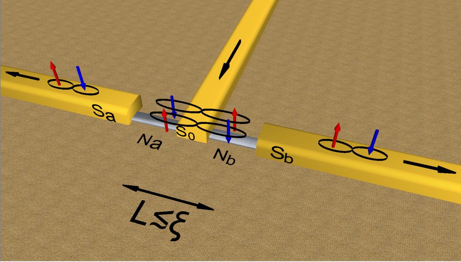
Figure 1: Artist view of a three-terminal Josephson junction, featuring the quartet resonance. $N_{a}$ and $N_{b}$ are two short metallic regions, small compared to the BCS coherence length $\xi$.

I Introduction

Multiterminal Josephson junctions have recently focused interest, as a generalization of standard two-terminal junctions. In particular, all-superconducting structures with three BCS superconductors $S_{a}$, $S_{b}$ and $S_{0}$ subject to voltages $V_{a}$, $V_{b}$ and $V_{0}$ (set to $V_{0}=0$ by convention) respectively (see Fig. 1) have been considered and revealed several types of resonances and threshold resonances if the DC currents are calculated as a function of voltages. The independent voltages $V_{a}$ and $V_{b}$ can be commensurate or incommensurate. For the realistic case of extended interfaces, the existence of two independent Josephson frequencies explains the absence of numerically exact results to this nonequilibrium transport problem. Yet, a number of new physical effects were obtained theoretically in different limiting cases (coherent or incoherent limit, ballistic or diffusive) and in different set-ups (metallic junctions or quantum dots, two or three interfaces).

The starting point was the discovery of what was called “self-induced Shapiro steps” by Cuevas and PothierCuevas-Pothier . This work was based on Usadel equations for a diffusive normal metal region connected to three superconductors, one of them involving a tunnel contact. DC resonances in the current were obtained at commensurate voltages. The analogy with Shapiro steps implies a zero-frequency mode-locking of the Josephson AC oscillations induced at the two transparent contacts. This reminds of the phenomenon studied in the ${}^{\prime}80s$ in well-separated junctions coupled by a non-mesoscopic environmentJillie . Later on, those resonances were rediscovered independently by Freyn et al.Freyn . A physical interpretation was uncovered in this work Freyn in terms of correlations among Cooper pairs in an intermediate virtual state located in the junction, extending within the coherence length in the superconducting leads. It was shown that these virtual states of Cooper pairs lead to entanglement if quantum dots are inserted into the three-terminal Josephson junction. The prototypical case involves opposite bias voltages $V_{a}=-V_{b}$ (with $V_{0}=0$) on terminals $S_{a}$ and $S_{b}$, which produces correlations among four fermions due to the exchange between two Cooper pairs (the so-called quartets, see Fig. 1). More generally, correlations among several Cooper pairs, coined as “multipair correlations” appear for commensurate $V_{a}$ and $V_{b}$ (e.g. if $V_{a}/V_{b}$ is a rational fraction). However, correlations among large numbers of Cooper pair are damped exponentially if the interfaces are not very transparent, because an additional electron-hole conversion amplitude crossing twice the interfaces is required to incorporate one more pair into a correlated Cooper pair cluster. Multipair correlations and related phenomena were explored recently by Jonckheere et al.Jonckheere for a double quantum dot connected to three superconductors. The lowest order quartet mode was understood in terms of splitting two Cooper pairs and recombining them in a way that involves an exchange between fermions. This mechanism leads to a minus sign in the phase dependence of the quartet current and is not captured by the heuristic ”synchronization” mechanism assumed by the Shapiro step analogy (the phase dependence was not studied in Ref.Cuevas-Pothier, ). Interestingly, another original process, coined as “phase-MAR” was discovered Jonckheere , corresponding to an interference term for multiple Andreev reflections (MARs), with transport of quasiparticles from one lead to another assisted by phase-sensitive quartets.

Two additional classes of threshold resonances have been unveiled by Houzet and Samuelsson Houzet-Samuelsson at the level of the quasiparticle conductance of incoherent MARs. Those threshold resonances are interpreted in terms of higher-order MAR channels involving all three terminals, which open upon reducing bias voltages. In this case, the ratio $V_{a}/V_{b}$ between the bias voltages can be commensurate or incommensurate.

Already at equilibrium, multiterminal superconducting structures possess striking properties, like Andreev states robustly crossing the zero-energy level Delft ; epjb ; Padurariu . The potential of such structures is exemplified in an intriguing proposal by Riwar et al. Riwar : it amounts to producing nontrivial topological effects due to Weyl fermions in a four-terminal all-superconducting structure probed with two small incommensurate voltages.

In contrast with all these predictions, very few experiments are presently available. In a pioneering transport experimentFrancois on a three-terminal long diffusive junction, clear Josephson-like anomalies have been observed at voltages corresponding to quartets emitted by one terminal towards the two others. More recent Shapiro step experiments on the same set-upDuvauchelle confirm the coherent character of these resonances. In such an experiment, the currents (and the conductance matrix) are obtained by fixing the voltages $V_{a},V_{b}$. Other experiments are expected in clean systems such as carbon nanotubes or nanowiresHeiblum defining quantum dots. Moreover, besides experiments controlling both voltages $V_{a},V_{b}$, one should envision experiments setting $V_{a}=-V_{b}=V$, which results in $\varphi_{Q}=\varphi_{a}+\varphi_{b}-2\varphi_{0}$ being a constant of motion. Because of the presence of three terminals, the voltage ($V$) and the phase ($\varphi_{Q}$) can be taken as two independant variables, and experiments are highly desirable in order to test the dependence of the quartet and MAR current with $V$ and $\varphi_{Q}$.

Yet, modeling such multichannel systems poses a formidable difficulty. The related work by Cuevas and PothierCuevas-Pothier is numerically exact, but one contact being a tunnel one. However, how about a situation in which all contacts have similar and intermediate transparency, as in the recent experiment by Pfeffer et al.Francois ? This question calls for treatments having the capability of dealing with this regime of intermediate transparency, which requires a fully nonperturbative approach. An alternative is to focus on a short disordered junction and use quantum circuit theoryPadurariu ; CircuitTheory , which is nonperturbative. Yet, this method also raises considerable difficulties for incommensurate voltages. More generally, it is difficult to obtain numerically exact results when two incommensurate frequencies and good extended interfaces are involved in the context of superconducting junctions, and this has not been done up to now. The paper by Cuevas et al.Cuevas-Shapiro on Shapiro steps in a one-channel superconducting weak link is one of the rare examples addressing a problem with two independent frequencies in the context of nanoscale superconducting junctions.

It is a general trend in the field of quantum electronics that experiments are controlled by robust effects that, up to now, have never required supercomputers for being uncovered theoretically at the semi-quantitative level. It is however true that the challenge of the exact solution may provide surprises in connection with nonlinear physics, but experimental relevance of those effects in the context of multiterminal Josephson junctions has not been proven at present time. Here, the line of thought is to ignore the effects appearing solely in the exact solution (e.g. not captured by the approximation used here), which does not prevent us from exploring the exact solution in the future, on the basis of large-scale numerical calculations.

The present paper proposes a kind of “unified” but approximate numerical framework for multiterminal Josephson junctions, which can be used for any ratio $V_{a}/V_{b}$ between the voltages (e.g. commensurate or incommensurate), as a substitute to the unavailable exact solution. The calculations are based on the so-called Hamiltonian approach [which was developed by Cuevas, Martín-Rodero and Levy YeyatiCuevas for multiple Andreev reflections in a single-channel superconducting weak link], and intermediate transparencies are used.

The method is developed for a three-terminal Josephson junction with two interfaces having the same intermediate transparency (see Fig. 2). It takes into account all multiple tunneling processes occurring separately at the interfaces but treats the scattering between interfaces (non-local processes) at lowest order, as if the distance between the interfaces was larger than the coherence length at all energies. Notice that this is never strictly true close to the gap edges where the penetration length of virtual quasiparticles becomes infinite.

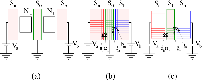
Figure 2: Schematics of the three-terminal superconducting junction. (a) shows thee same $SNSNS$ set-up as Fig. 1. (b) shows a two-dimensional tight-binding model in which the short normal regions are modeled by a tight-binding tunnel amplitude with intermediate transparency. (c) shows the considered model in which $S_{a,b}$ are made of a collection of one-dimensional channels, thus avoiding the discussion of nonlocal effects in the leads $S_{a,b}$.

Within this approximation, all resonances at rational $V_{a}/V_{b}$ can be captured in a semi-quantitative way, and the MAR threshold resonancesHouzet-Samuelsson are also obtained for irrational $V_{a}/V_{b}$. The method can eventually be generalized to four-terminal structures. Agreement with respect to results established previously Houzet-Samuelsson ; Freyn ; Jonckheere is obtained, and the numerical results are thoroughly discussed on a physical basis, especially in connection with the recent experiment by Pfeffer et al.Francois . Other points of comparison with known behavior will be obtained. For instance, in agreement with Jonckheere et al.Jonckheere , the current-phase relation has the correct sign for the first phase-sensitive resonances. In agreement with the predominance of normal electron transmission over nonlocal Andreev reflection in a normal metal-superconductor-normal metal junction ($NSN$)Melin-Feinberg , the critical current is larger in absolute value for identical voltages (direct transfer of pairs from $S_{a}$ to $S_{b}$ through $S_{c}$, coined asFreyn “pair cotunneling”) than for opposite voltages (the so-called quartets, also called as double nonlocal Andreev reflectionFreyn ). In addition, deviations from harmonic current-phase relation are stronger for larger interface transparency and higher bias voltage. This reminds of the results of a Blonder-Tinkham-KlapwijkBTK calculation for a $NS$ junction, in which the subgap current increases with voltage at intermediate transparency. An interesting physical result on three-terminal junctions will conclude our study, regarding the relative magnitude of quartets and multipairs with respect to the MAR signal at intermediate transparency. Indeed, the multipair and quartet resonances can have a large “critical” current in comparison to the background MAR current. Therefore they can have a high visibility compared to the quasiparticle background and lead to a current signal that can be large enough for experimental detection in a voltage-biased measurement, which is compatible with the experiment by Pfeffer et al.Francois . This conclusion raises the question of whether multipair resonances also have high visibility in comparison to quasiparticles in the four-terminal set-up proposed recently by Riwar et al.Riwar . At least in which region of the $(V_{a},V_{b})$ plane is the experimental signal dominated by Weyl fermion-like effects or by multipair resonances ?

The article is organized as follows. Introductory material on the method is presented in Sec. II, all analytical calculations being relegated to Appendices. The numerical results are presented and interpreted in Sec. III, in connection to previous resultsFreyn ; Houzet-Samuelsson ; Jonckheere and to a recent experiment by Pfeffer et al.Francois . Concluding remarks are presented in Sec. IV.

II Introduction to the method

II.1 The set-up

Set-ups containing three interfaces are considered in some theoretical approaches, such as the Usadel equations used by Cuevas and Pothier Cuevas-Pothier , circuit theory treated by Padurariu et al.Padurariu ; CircuitTheory , or the single quantum dot connected to three superconductors treated by Mélin et al. (work in progress). Other approaches consider two superconductors $S_{a}$ and $S_{b}$ at voltages $V_{a}$ and $V_{b}$ connected to the grounded $S_{0}$ (see Fig. 2), thus with only two interfaces. This includes Freyn et al.Freyn , Jonckheere et al.Jonckheere , with the possibility of a direct coupling between the two interfacesepjb . In the Grenoble experiment Francois , one sample has three interfaces, and another “reference” sample close to Fig. 1 contains only two $SNS$ junctions. For the latter, the separation between interfaces is larger than the superconducting coherence length, which explains why quartets are not visible in the set-up having only two interfaces. However, there is no technical impossibility to achieve experimentally another sample with only two interfaces separated by a few superconducting coherence lengths. With two interfaces, nonlocal effects at the scale of the coherence length can be neglected in $S_{a}$ and $S_{b}$ but of course not in $S_{0}$. The avaible experimental data obtained in this Grenoble experiment Francois do not strictly speaking correspond to the same conditions as those corresponding to the calculations presented below: the experiment is in the diffusive limit for a long junction, and the geometry is not identical.

In what follows, the interfaces $S_{a}S_{0}$ and $S_{b}S_{0}$ are extended (multichannel), and $S_{a}$ and $S_{b}$ are thus separately connected to $S_{0}$, forming a three-terminal Josephson junction with only two interfacesFreyn (see Fig. 2). The normal metallic regions $N_{a}$ and $N_{b}$ are treated in the short junction limit, and are approximated by a hopping amplitude $\Sigma_{0}$, taken for simplicity as uniform over the junctions. Strictly speaking, $S_{a}$, $S_{b}$ and $S_{0}$ are modelled as a collection of independent one-dimensional channels in which the mean-field BCS superconducting gap is supposed to be uniform. This assumption is reasonable, even for $S_{0}$ which is macroscopic except in the contact region. A decrease of the gap in $S_{0}$, due to proximity effect could easily be included in the theory, but a fully self-consistent calculation in the spirit of Ref. Melin-Bergeret-Yeyati, seems to be out of reach at present time.

The current $I_{a,\alpha}$ connecting two points $a$ (in $S_{a}$) and $\alpha$ (in $S_{0}$) is calculated (see Appendix A and Fig. 2), then integrated on the contact area. Within a tunnel Hamiltonian, each elementary tunnel event connects to only one pair of points $(a,\alpha)$ and the total current scales linearly with the contact area (or the number of channels). This holds even if multiple tunneling takes place, as in the present nonperturbative calculation. In what follows, the currents per channel are plotted. The calculation uses a tight-binding Hamiltonian [see Eqs. (A.1)-(7)]. Such a two-dimensional model for a $NSN$ junction in strong nonequilibrium conditions was treated numerically by Mélin, Bergeret and Levy YeyatiMelin-Bergeret-Yeyati with recursive Green’s function. A similar assumption was made (e. g. neglecting nonlocal effects in the leads), and this simplifying assumption did not produce noticeable artifacts on the current. As it was the case for nonlocal transport at a $NSN$ interface Melin-Feinberg-EPJB ; Melin-Feinberg ; Melin-Bergeret-Yeyati , the superconducting electrodes $S_{a}$ and $S_{b}$ are modelled as a collection of one-dimensional channels, connected to the two-dimensional superconductor $S_{0}$. Our theoretical approach Falci ; Melin-Feinberg-EPJB ; Melin-Feinberg ; Melin-Bergeret-Yeyati has proven to be successful to capture the relevant experimental physicsBeckmann ; Russo ; Cadden and this is why we continue here this theoretical description into the field of three-terminal Josephson junctions.

The calculation is performed by using as control parameters the voltages $V_{a}$, $V_{b}$ and the phases at the origin of time $\varphi_{a},\varphi_{b},\varphi_{0}$. Contrarily to two-terminal junctions, these phases play an essential role in DC transport because on a line $pV_{a}+qV_{b}=0$ ($p,q$ integers), they lead to a constant of motion $p\varphi_{a}+q\varphi_{b}-(p+q)\varphi_{0}$. This becomes in turn a potential control parameter in an experiment.

The tight-binding hopping amplitude in the bulk of $S_{a}$, $S_{b}$ and $S_{0}$ is denoted by $W$. The interface transparency is characterized by the dimensionless transmission coefficient (in between $0$ and $1$) and is equal to $T_{N}\simeq 4\Sigma_{0}^{2}/W$ if $\Sigma_{0}$ is small compared to $W$ (small interface transparencies). The tunnel junctions realized in experiments correspond typically to $T_{N}\simeq 10^{-4}$. Much larger intermediate values $T_{N}\simeq 0.04\div 0.33$ are used in the following numerical calculations, corresponding to intermediate interface transparencies. These achieve a compromise between the presence of a MAR structure that will turn out to develop [allowing to access a significant number of MAR threshold resonances Houzet-Samuelsson ], and a sufficiently weak subgap quasiparticle current [allowing multipair resonances in the current to have sufficient visibility compared to the quasiparticle background current signal]. Notice that the recent experiment by Pfeffer et al. Francois is done with intermediate interface transparencies (about $0.3$).

II.2 Symmetries of the current from microscopic calculations

We start by investigating the symmetries of the current, in order to demonstrate compatibility of the Hamiltonian approach with expectations based on general symmetry arguments Jonckheere . The corresponding calculations are relegated in the Appendices. [An introduction to the Green’s functions calculations is provided in the Appendix A; an analysis of the symmetries of the current is provided in Appendix B]. The strategy is to obtain symmetries for the bare Green’s function, to be “transferred” to the fully dressed advanced and retarded Green’s functions, and next to the Keldysh Green’s function and to the current. The conclusion is a confirmation of the arguments by Jonckheere et al.Jonckheere that the current originates from two terms with different parities with respect to phase and voltage reversal. Indeed, it was shown previouslyJonckheere on the basis of time-reversal combined to particle-hole symmetry that $I(V_{i},\varphi_{j})=-I(-V_{i},-\varphi_{j})$. Written in the form of Eq. (45), here the current is explicitly decomposed into a term that is odd in phase – and thus even in voltage – (the multipair component, including the quartet current for opposite voltages), and into a term that is odd in voltage – and thus even in phase – (the phase-MAR current). In the voltage range considered in what follows, only the contribution to the current which is even in voltage and odd in phase contributes to the phase-sensitive current at a multipair resonance: the voltages considered in Sec. III are mostly below threshold for the appearance of the phase-MAR processes corresponding to the other parity Jonckheere .

II.3 Perturbative expansion in the number of nonlocal bare Green’s functions

A breakdown of perturbation theory in interface transparency for the current already appears at the level of the Blonder-Tinkham-KlapwijkBTK (BTK) wavefunction calculation of the Andreev reflection current in a normal metal-insulator-superconductor ($NIS$) junction. It is underlined that the following argument is for a single $NIS$ interface, with a time-independent Hamiltonian. A one-dimensional model of $NIS$ junction is considered now, with a dimensionless interfacial scattering potential $Z$, according to the standard BTK notationBTK . Perfectly transparent junctions correspond to $Z=0$, and tunnel contacts to $Z\gg 1$. An expansion in $1/Z\ll 1$ of the transmission coefficient is carried out now (namely, a small-transparency expansion) and, in a second step, the integral over energy of each term of this expansion will be evaluated from $0$ to $eV$. This procedure is problematic if $eV$ becomes larger than the superconducting gap $\Delta$, in which case the gap edge singularity is within the interval of integration over energy $E$. [In the discussion of the BTK calculation, the energy is denoted by $E$ as in usual BTK calculations. The symbol $E$ has the same meaning as $\omega$ used in the Green’s function calculations.]

The BTK amplitudes BTK $A(E)$ (Andreev reflection) and $B(E)$ (normal reflection) are expanded as follows in $1/Z$, with $Z\gg 1$:

$$A(E) = \frac{u_{0}^{2}v_{0}^{2}}{(u_{0}^{2}-v_{0}^{2})^{2}Z^{4}}+\frac{2u_{0}^{2}v_{0}^{2}}{(-u_{0}^{2}+v_{0}^{2})^{3}Z^{6}}$$

$$+ {\cal O}\left(\frac{1}{Z^{8}}\right)$$

$$B(E) = 1+\frac{1}{Z^{2}}\left(1-\frac{2u_{0}^{2}}{(u_{0}^{2}-v_{0}^{2})^{2}}\right)$$

$$+ \frac{1}{Z^{4}}\left(\frac{3u_{0}^{4}}{u_{0}^{2}-v_{0}^{2}}-\frac{2u_{0}^{2}}{u_{0}^{2}-v_{0}^{2}}\right)+{\cal O}\left(\frac{1}{Z^{6}}\right),$$

where $u_{0}$ and $v_{0}$ denote the BCS coherence factors for electrons and holes. Specializing to $E\simeq\Delta$ leads to

$$A(E) \simeq \frac{\Delta^{2}}{4(E^{2}-\Delta^{2})}\frac{1}{Z^{4}}$$

$$+ \frac{1}{4}\left(\frac{\Delta^{2}}{E^{2}-\Delta^{2}}\right)^{3/2}\frac{1}{Z^{6}}+...$$

$$B(E) \simeq 1-\frac{1}{Z^{2}}\left(\frac{\Delta^{2}}{E^{2}-\Delta^{2}}\right)^{1/2}$$

$$+ \frac{3}{4Z^{4}}\frac{\Delta^{2}}{E^{2}-\Delta^{2}}+....$$

Perturbation theory in $1/Z$ for the spectral current $1+A(E)-B(E)$ is ill-defined in the window $E\in[\Delta(1-\alpha Z^{-4}),\Delta(1+\alpha Z^{-4})]$, where $\alpha$ is a constant of order unity. Divergences are produced in the energy dependence of the spectral current, leading to an expression of the current integrated over energy as the sum of an infinite number of infinite terms, which, eventually, takes the finite value obtained by BTK BTK in the nonperturbative theory. Thus, perturbative expansions of the current produce non physical divergences if the gap edge singularities are included in the energy integration interval.

A similar artifact is present in the forthcoming partially resummed perturbation theory for a three-terminal junction. In this case, the exact nonperturbative values of the currents are unreachable, because of far too long times for their computation. It is emphasized that, because of multichannel effect, even at a multipair resonance (such as the quartet resonance), where only one frequency remains in the calculation, it is not an easy task to obtain the fully nonperturbative value of the current. On the other hand, the lowest order term turns out to diverge only logarithmically. This lowest-order term will be shown to behave correctly with respect to physical expectations and to the results established over the last few years for the quartet, multipairFreyn ; Jonckheere and MAR currents Houzet-Samuelsson . The message is that, in practice, partially resummed perturbation theory can be used at lowest order to understand the features of experiments.

The approach relies on the same principle as a previous work by Mélin and FeinbergMelin-Feinberg in the context of nonlocal transport in a $NSN$ junction, in connection with a crossover of the nonlocal conductance from negative to positive as interface transparency is increased. The idea of the method is to solve exactly the structure with two interfaces sufficiently remote so that they can be considered as independent. Then, the current is evaluated as the interfaces are made closer, but still at a distance of the order of a few coherence lengths. This amounts to make an expansion in the strength of the processes connecting both interfaces, which, technically, relies on an expansion of the current in the number of back-and-forth amplitudes (e.g. the nonlocal bare Green’s functions) connecting the interfaces. The technical implementation is more complex in the case of an all-superconducting device, because of the time-dependence of the Hamiltonian, but the principle of the calculation is exactly the same. Such perturbation theory in the number of nonlocal Green’s functions converges well in the work mentioned above Melin-Feinberg on nonlocal transport in a $NSN$ structure: for applied voltage much smaller than the gap, $\exp[-R/\xi(0)]$ is the small parameter in this expansion even at high transparency, where $R$ is the separation between interfaces, and $\xi(0)$ is the zero-energy coherence length. One of the interests of what follows (going against what may be pessimistically anticipated at first glance) is to show that physically useful and relevant (even though not mathematically exact) information can be extracted from a similar expansion in an all-superconducting set-up. Intermediate transparency will be used, which has the effect of cutting off high-order terms in the tunnel amplitude, except in a spectral window close to the gaps. Roughly speaking, in the all-superconducting case, the parameter of the perturbative expansion becomes $\exp[-R/\xi(\omega)]$, which is of order unity if the energy $\omega$ (with respect to the chemical potential of $S_{0}$) is close to the gap in the energy integral of the phase-sensitive spectral current: the finite-energy coherence length $\xi(\omega)$ diverges as $\omega\rightarrow\Delta$. Divergences in the superconductor density of states are also present in the gap edge spectral window, which explains why the formal breakdown of perturbation in the number of nonlocal Green’s function deserves special discussion for the considered all-superconducting structure. Let us underline that this approach is not equivalent to the tunnel approximation for the $S_{0}$ interface, as used by Cuevas and Pothier Cuevas-Pothier . Indeed, our calculation treats part of the multiple scattering events at this interface. On the contrary, in Ref.Cuevas-Pothier, , the superconductors $S_{a},S_{b}$ are directly coupled in a nonperturbative way through the normal region.

In a more technical language, each microscopic process contributing to the DC current at order-$2n$ corresponds to a closed diagram having $2n$ nonlocal bare Green’s functions crossing the central superconductor $S_{0}$. With this convention, the lowest order in partially resummed perturbation theory is order-two in the number of nonlocal Green’s functions. The next-order terms is order-four, … The Dyson equations provide a perturbation series in the hopping amplitude $\Sigma_{0}$. This series in power of $\Sigma_{0}$ will be reordered as a series in the number of nonlocal bare Green’s functions, taking into account to all orders dressing by “local” processes [e.g. each of those processes involves only one of the two $S_{0}S_{a}$ or $S_{0}S_{b}$ interfaces, without coupling to the other]. Said differently in a more physical picture, at lowest order, an electron-like quasiparticle coming from $S_{a}$ couples to MARs to all orders at the $S_{a}IS_{0}$ interface. Next, it can experience electron-hole conversion while crossing $S_{0}$ only once, and finally, the resulting hole-like quasiparticle is subject to MARs at the $S_{0}IS_{b}$ interface before being transmitted into $S_{b}$. Combining with a similar processes from $S_{b}$ to $S_{a}$ leads to physical picture for the history of the $n=1$ processes contributing to the lowest order-two approximation for the phase-sensitive current at a multipair resonance.

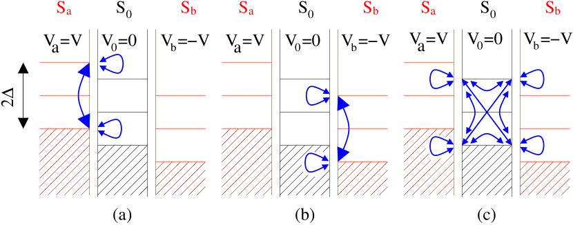
Figure 3: Schematics of the three resonances in a three-terminal $S_{a}IS_{0}IS_{b}$ junction biased at opposite voltages $V_{a}=-V_{b}\equiv V$. Resonances (a) and (b) are summed to all orders by the Dyson equations. Resonance (c) is not resummed, and it is responsible for divergences in perturbation in the number of nonlocal bare Green’s functions. The arrows denote bare Green’s functions. All arrows starting and ending at the same energy correspond to energy-conserving normal electron transmission, and the arrows connecting opposite energies (with respect to the chemical potential) correspond to an electron-hole amplitude.

Fig. 3 shows the three processes resonating at the gap edges, in the simplifying case of opposite bias voltages (quartet resonance). Both processes on panels a and b take place “locally”, and they connect energies $\pm\Delta+eV$ and $\pm\Delta-eV$ at which the density of states diverges in $S_{a}$ and $S_{b}$ respectively. Those divergences need to be regularized by inversion of the part of the Dyson matrix describing processes taking place locally at each interface. Conversely, the resonance on Fig. 3c will be treated perturbatively, and it is this resonance which is responsible for divergences in perturbation in the number of nonlocal Green’s functions, if the gap edge of the superconductor $S_{0}$ is within the energy integration interval. Recipes were attempted for approximate resummations of the process on Fig. 3c. Those resummations are not presented here because it was not possible to estimate the gain in accuracy on the value of the currents with respect to what follows. The remainder of the analytical calculations turns out to be too technical for being presented in the main body of the article. Appendix C summarizes those calculations. Details on the numerical implementation are provided in Appendix D.

III Results

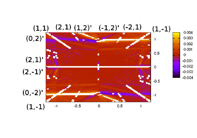
Figure 4: Threshold resonances in the nonlocal conductance per channel $\partial I_{a}^{qp}/\partial V_{b}$, in the $(V_{a}/\Delta,V_{b}/\Delta)$ plane (in units of $e^{2}/h$ to provide typical orders of magnitude with a gap $\Delta=10^{-3}W$, still two orders of magnitude larger than a realistic ratio of $\sim 10^{-5}$). The value $N_{max}=6$ is used for the cut-off on the number of harmonics of the Josephson frequency, and almost indistinguishable data were obtained for $N_{max}=7,8,9$. The dimensionless normal state transmission at each of the $S_{a}S_{0}$ and $S_{b}S_{0}$ interfaces is $T_{N}\simeq 0.33$. The separation between the contacts is $R/\xi_{0}=2$, where $\xi_{0}$ is the low-energy coherence length. The phases are $\varphi_{a}-\varphi_{0}=\varphi_{b}-\varphi_{0}=0$. The white pixels are pronounced MAR threshold resonances that fall out of the color-scale. The resonant thresholds denoted by $(p,q)$ correspond to $pV_{a}+qV_{b}=0$ in Eq. (5), and those denoted by $(p^{\prime},q^{\prime})^{\prime}$ correspond to $p^{\prime}V_{a}+q^{\prime}V_{b}=2\Delta/e$. The resonant thresholds $(0,3)^{\prime}$, $(0,-3)^{\prime}$, $(1,3)^{\prime}$ and $(1,-3)^{\prime}$ are also visible on the figure.

As a first point of comparison for partially resummed perturbation theory, the set of MAR threshold resonances discovered by Houzet and SamuelssonHouzet-Samuelsson was recovered for incommensurate voltages (however, in the phase-coherent case as far as the present calculations are concerned). Those threshold resonances correspond to two families associated to the opening of the channels of MARs:

$$pV_{a}+qV_{b}=0,\mbox{and }p^{\prime}V_{a}+q^{\prime}V_{b}=\frac{2\Delta}{e},$$ (5)

with $p,q$ and $p^{\prime},q^{\prime}$ four integers. The question arises of whether all values of ($p,q$) are accessible within lowest order-two in the number of nonlocal Green’s functions. The answer is that a $(p,q)$ diagram for multipairs can be transformed into a $(p,q)$ diagram for phase-sensitive MARs by adding one extra line. One easily checks that some multipairs diagrams can be constructed by using only two nonlocal lines. Yet, they involve only two split pairs from $S_{0}$, and for higher order processes (sextets, octets..) e.g. if $p>1$ or $q>1$, the other pairs participating to the multipair correlation are not split but originate from direct Andreev reflection at the $N_{a}$ or $N_{b}$ interface. The above considerations show that at lowest order in the nonlocal processes, all values of $(p,q)$ are expected to be accounted for, however approximately. At higher order (not treated hereafter), two, three or higher numbers of Cooper pairs may split, also accompanied by a $(p,q)$ multipair at both interfaces. Fig. 4 is a color-plot showing the dependence on $V_{a}/\Delta$ and $V_{b}/\Delta$ of the nonlocal conductance, the phases being set to zero. This ensures that the multipair current (odd in phase) occurring for commensurate voltages is zero and that the calculated features are solely due to MAR quasiparticle transport. With the intermediate transparency used here ($T_{N}\simeq 0.33$), those threshold resonances appear essentially above a voltage range set by the superconducting gap.

The contact transparencies are also intermediate in the recent experiment by Pfeffer et al. on three-terminal metallic structures Francois . The result for the MAR threshold resonances is thus compatible with the fact that those threshold resonances were not observed at low bias in this work (due also to inelastic cutoff of high order MAR). On the other hand, this experiment could not probe voltages comparable to the gap, which would be a requirement for probing the MAR threshold resonances visible on Fig. 4.

Interestingly, positive nonlocal conductance $\partial I_{a}/\partial V_{b}$ is obtained in Fig. 4 (see also the forthcoming Fig. 7) for some of those MAR threshold resonances, with the same sign as Cooper pair splitting. This appears to be reminiscent of the possibility of positive cross-correlations of MAR currents in a three-terminal all-superconducting hybrid junction Duhot . On the other hand, in a $NSN$ three-terminal junction, the positive nonlocal conductance at small transparency changes into negative nonlocal conductance at high transparency Melin-Feinberg , suggesting that, at an oversimplified level ignoring the condensates while retaining only Cooper pair splitting, the effective transparency would depend on how remote the voltages are from threshold resonances. However, this mechanism is not directly relevant to the calculations presented here because, even at the MAR threshold resonances, the nonlocal conductance per channel is weak (see Fig. 4), thus with underlying microscopic processes operating in the perturbative regime. The prediction of MAR threshold resonances with positive nonlocal conductance is interesting for the prospect of future experiments and theoretical calculations aiming at an evidence for voltage-controlled positive non local-conductance.

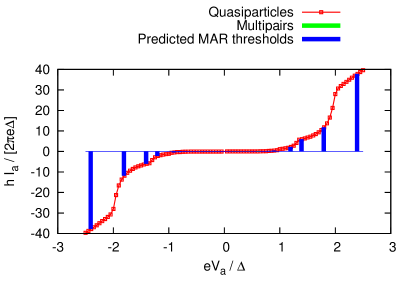
Figure 5: MAR structure in $I_{a,qp}$ as a function of $V_{a}$ for fixed $V_{b}$, with $N_{max}=6$. Convergence was verified by comparing to $N_{max}=7,8,9$. The dimensionless transmission coefficient is $T_{N}\simeq 0.33$. The value $eV_{b}=0.6\Delta$ is used, as well as $\Delta\equiv\Delta_{a}=\Delta_{b}=\Delta_{0}=10^{-3}W$. The multipair resonances are also drawn, but they are not visible on this scale. The blue impulses show the first MAR threshold resonances. The value $R/\xi_{0}=2$ was used.

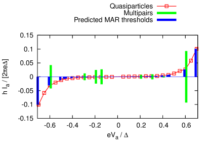
Figure 6: The same as Fig. 5, but now in a restricted voltage range. The green impulses show the resonances in the phase-sensitive component of the current at $V_{a}=(p/q)V_{b}$, with $1\leq p\leq 4$ and $1\leq|q|\leq 4$. The size of each green impulse corresponds to the maximum over the superconducting phase $\varphi_{0}$ of the absolute value of the current at each considered multipair resonance. The blue impulses on panel a have the same meaning as in Fig. 5, they correspond to the MAR threshold resonances Houzet-Samuelsson . The value $eV_{b}=0.6\Delta$ is used, as well as $\Delta\equiv\Delta_{a}=\Delta_{b}=\Delta_{S}=10^{-3}W$ and $\Sigma_{0}/W=0.3$. The value $R/\xi_{0}=2$ was used.

The MAR threshold resonances are better visualized on Fig. 5 featuring the quasiparticle current $I_{qp}$ as a function of $V_{a}$ for a fixed $eV_{b}/\Delta=0.6$, with $V_{a}$ and $V_{b}$ incommensurate. The quasiparticle current as a function of $V_{a}$ is dominated by the contribution of the $S_{a}S_{0}$ interface, not by the smaller contribution of the processes coupling the two interfaces. The first MAR threshold resonance Houzet-Samuelsson deduced from the relations (5) coincide with thresholds in the structure for the current plotted as a function of voltage. The cut-off $N_{max}$ in the space of the harmonics of the local Green’s functions is varied systematically, keeping only the value $N_{max}=6$ on Fig. 5. Indistinguishable data were obtained for $N_{max}=7,8,9$ (not shown here), demonstrating convergence with $N_{max}$. This excellent convergence is due to the intermediate value of $T_{N}=0.33$ between the superconductors.

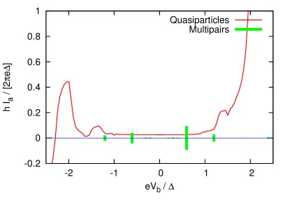
Figure 7: The figure shows the MAR structure in $I_{a}$ as a function of $V_{b}/\Delta$ for fixed $V_{a}/\Delta=0.6$, and with $N_{max}=6$. Convergence with respect to $N_{max}=7$ was verified. The normal state transmission coefficient is $T_{N}\simeq 0.33$. All gaps are identical: $\Delta\equiv\Delta_{a}=\Delta_{b}=\Delta_{S}=10^{-3}W$. The green lines show the value of the critical current of the first multipair resonances. The value $R/\xi_{0}=2$ was used on the figure.

Fig. 6 shows the same data on a more restricted voltage range smaller than the gap. The multipair resonances are shown by green impulses on this figure. To obtain those resonances, the current-phase relation $I_{multipairs}(\varphi_{a},\varphi_{b})$ was evaluated as a function of $\varphi_{b}$ for $\varphi_{a}=\varphi_{0}=0$ and the absolute value of the critical current (maximum value of the current) was reported on the figure by an impulse. Similarly to a Josephson current, or Shapiro steps, a conserved phase variable (here $\varphi_{0}$ if choosing $\varphi_{a}=\varphi_{b}=0$) underlies the multipair current along these green impulses. Multipair resonances have distinguishing features at $pV_{a}+qV_{b}=0$, associated to the phase-sensitive component of the current ($p=q=1$ corresponds to the quartets). The value of the multipair critical current at resonance is much larger than the quasiparticle current, therefore making the observation of the quartet and multipair resonances possible at intermediate transparency. The same data are shown on Fig. 7 as a function of $V_{b}$ for a fixed value of $eV_{a}=0.6\Delta$. The non-uniform part of the quasiparticle signal on Fig. 7 corresponds solely to the “crossed” or “nonlocal” current response of $I_{a}$ through $S_{a}$ as a function of voltage $V_{b}$ on $S_{b}$, therefore providing evidence for microscopic processes coupling nontrivially the two interfaces. More precisely, the current $I_{a}$ is calculated according to the approximations presented in the Appendices, and the derivative in the nonlocal conductance $G_{a,b}=\partial I_{a}/\partial V_{b}$ is evaluated numerically. The background current (with respect to the multipair resonances) due to local quasiparticle current at the $S_{a}S_{0}$ interface is not small, and local maxima associated to the MAR threshold resonances are visible. A significant contrast for the multipair resonances out of the background of MARs is obtained even for the relatively high value $eV_{a}/\Delta=0.6$, not being a tiny fraction of the gap. Those features are consistent with the recent experiment Francois in which resonances were obtained in the $(V_{a},V_{b})$ parameter space, consistent with quartets. Higher-order resonances are not reported in this experiment Francois , whereas multipairs have a non-negligible weight in the calculations presented here. It would be interesting to know whether future experiments would provide evidence for higher-order resonances.

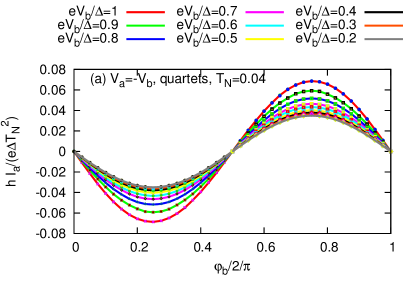
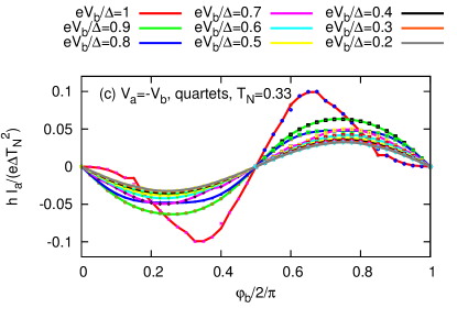
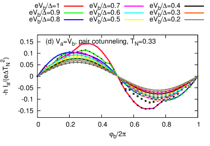
Figure 8: Current-phase relation for $I_{a}(\varphi_{b})$ for $V_{a}=-V_{b}$ (quartets, panels a and c), and $-I_{a}(\varphi_{b})$ for $V_{a}=V_{b}$ (pair cotunneling, panels b and d). The currents are normalized to $(e\Delta/h)T_{N}^{2}$, which explains that the currents for $T_{N}\simeq 0.04$ (panels a and b) are roughly on the same scale as those for $T_{N}\simeq 0.33$ (panels c and d). The figure shows the phase-sensitive component of the currents $I_{a}$ (or $-I_{a}$) as a function of $\varphi_{b}$ for $\varphi_{a}=\varphi_{0}=0$ for the values of $eV_{b}/\Delta$ shown on the figure. All data-points for $N_{max}=4,5,6$ (for $T_{N}\simeq 0.04$) and $N_{max}=7,8,9$ (for $T_{N}\simeq 0.33$) are shown on the figure, which provides evidence for excellent convergence as the cut-off $N_{max}$ on the number of harmonics of the Josephson frequency is increased. The three gaps are identical ($\Delta\equiv\Delta_{a}=\Delta_{b}=\Delta_{S}=10^{-3}W$).

Fig. 8 (for $T_{N}=0.04$ and $T_{N}=0.33$, and for $V_{a}=V_{b}$ and $V_{a}=-V_{b}$) shows the current-phase relations $I_{multipairs}(\varphi_{a},\varphi_{b})$ as a function of $\varphi_{b}$ for $\varphi_{a}=\varphi_{0}=0$, at the resonances associated to $V_{a}=-V_{b}$ (quartetsFreyn , panels a and c), and to $V_{a}=V_{b}$ (pair cotunnelingFreyn amounting to transferring pairs from $S_{a}$ to $S_{b}$ , or vice-versa, panels b and d). The larger value (in absolute value) of the critical current of pair cotunneling compared to that of quartets is at odds with the results obtained by Jonckheere et al.Jonckheere for quantum dot calculations in the metallic regime. If $k_{F}$ is the Fermi wave-vector and $R$ the distance between the point contacts, a very specific value $k_{F}R=2\pi m$ (with $m$ and integer) was used in this previous work Jonckheere . According to the theory of nonlocal transportFalci ; Melin-Feinberg ; Melin-Feinberg-EPJB , this assumption of strict zero-dimensionality is not reliable for extended interfaces, for which all possible values of $k_{F}R$ are to be taken into account [see the form of the nonlocal Green’s function in Eq. (16) that is definitely different in the cases of generic $k_{F}R$ and specific value $k_{F}R=2\pi m$]. This effect on the magnitude of the critical current for opposite or identical voltages is due solely to higher-order terms in the tunnel couplings [a perfect symmetry between the critical currents of quartets and elastic cotunneling was obtained by Freyn et al.Freyn in the tunnel limit $T_{N}\ll 1$]. It is concluded that the treatment of higher order terms in the tunnel amplitudes presented here is sufficient for obtaining physically sound behavior: the predominance of pair cotunneling over quartets is reminiscent of that of normal electron transmission over Cooper pair splitting in a three-terminal $NSN$ junction, a result first obtained in Ref. Melin-Feinberg, .

It is clear from Fig. 8 that the plots of $I_{a}(\varphi_{b})$ with $\varphi_{a}=\varphi_{0}=0$ are compatible with a $\pi$-shift of the quartet current at opposite bias voltages, absent for pair cotunneling current at identical bias voltages. Indeed, the current-phase relation in the adiabatic limit takes the following form for the quartets: $I_{a}=-|I^{Q}|\sin(\varphi_{a}+\varphi_{b}-2\varphi_{0})=-|I^{Q}|\sin(\varphi_{b})$. The minus sign ($\pi$-shift) is a signature of the lowest-order quartet diagram. Pair cotunneling instead leads to $-I_{a}=-|I^{dEC}|\sin(\varphi_{a}-\varphi_{b})=|I^{dEC}|\sin(\varphi_{b})$, and there is no $\pi$-shift in this case. Here, $I^{Q}$ and $I^{dEC}$ generalize the usual critical current found at equilibrium. Again, partially resummed perturbation theory is compatible with physical expectations: the original inversion of the sign of the current-phase relation for the quartets is related to the electron exchange between two Cooper pairs in the quartet process Jonckheere .

One also notices that the nonharmonic behavior in the current-phase relation is enhanced as the normal-state transmission increases from $T_{N}=0.04$ to $T_{N}=0.33$ (see Fig. 8), or as voltage becomes closer to the gap of $S_{0}$, which is a behavior expected on physical grounds. The proposed interpretation is that the subgap current at intermediate transparency increases as the bias is increased towards the superconducting gap, making the junction effectively more transparent, as in a BTK calculation BTK for a $NS$ interface.

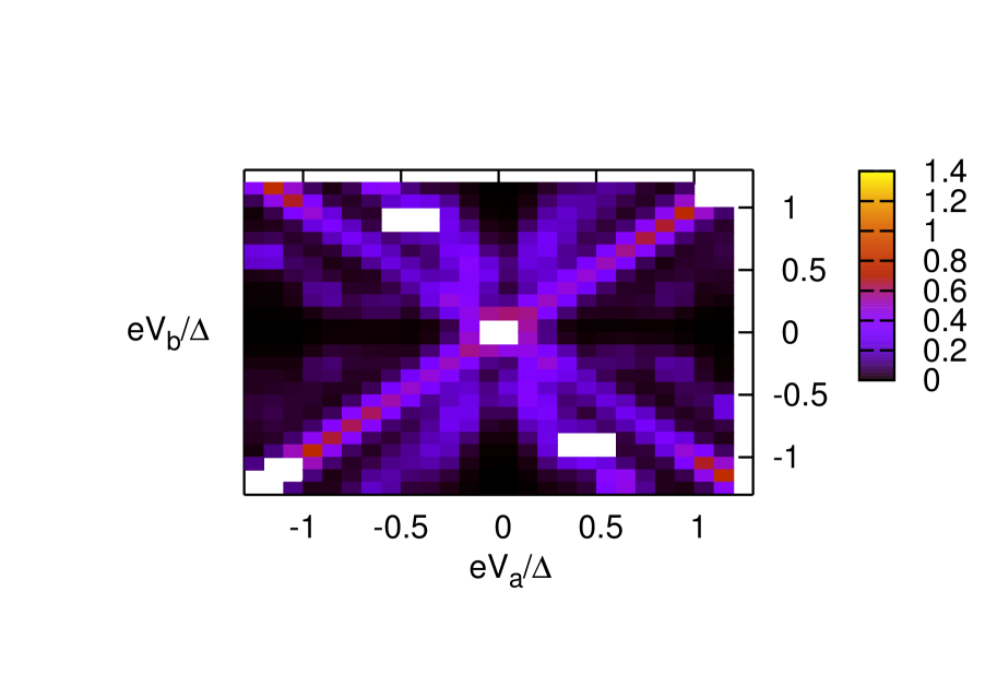
Figure 9: The figure shows the absolute value of the total quartet critical current (in color-scale) as a function of $eV_{a}/\Delta$ and $eV_{b}/\Delta$, with $N_{max}=9$ as a cut-off on the number of harmonics of the Josephson frequency. Indistinguishable figures were obtained for $N_{max}=6,7,8$, which demonstrates convergence. The three gaps are identical ($\Delta\equiv\Delta_{a}=\Delta_{b}=\Delta_{S}=10^{-3}W$). The normal-state transmission coefficient is $T_{N}=0.33$. The value $R/\xi_{0}=2$ was used on the figure. The current is normalized to $(e\Delta/h)T_{N}^{2}$. The pixels in white are out of the color-scale.

Broadening of the multipair resonances was introduced “by hand” in Fig. 9, with the (modest) motivation of making the numerical data look closer to experiment by Pfeffer et al. Francois where an important broadening is present. The parameter $\eta$ alone, as it is introduced in our calculations, is not sufficient for generating such width. Strictly speaking, a finite width for the resonance in the $(V_{a},V_{b})$ plane is difficult to understand in the case of strict voltage bias: as soon as $V_{a}+V_{b}\neq 0$, then $\varphi_{a}+\varphi_{b}-2\varphi_{0}$ starts to become time-dependent. The finite width is introduced here to mimic an environment with finite impedance. The color-map in Fig. 9 underlines similarities and differences with the experimental dataFrancois . The main difference is that all superconducting terminals are equivalent in this experiment, and this is not the case in the set-up on which the present calculations are carried out. Considering an interpretation of this experiment in terms of quartets would mean that the latter can be emitted by the three equivalent superconducting leads in the experiment, according to the values of the voltages. As a result, three equivalent lines are obtained experimentally in the $(V_{a},V_{b})$ plane, which are compatible with an interpretation in terms of quartets. However, the three superconducting leads are not equivalent in the set-up used in the present calculations in which quartets are emitted solely from the grounded $S_{0}$, leading to a single resonance line at $V_{a}+V_{b}=0$ for the quartets. The other lines in Fig. 9 correspond to multipair correlations among a larger number of pairs (sextets, octets, …)

IV Conclusions

An efficient approximate analytical and numerical framework was provided for a three-terminal Josephson junction. This framework is based on semi-analytical calculations suitable for providing a kind of “unified” picture for the various phenomena taking place in a three-terminal superconducting junction. The principle of the method was presented, and it was demonstrated that this method reproduces the behavior of the various resonances and threshold resonances discovered over the last few years Freyn ; Houzet-Samuelsson ; Jonckheere , as well as several features, especially those related to the current-phase relation. It was demonstrated that MARs and multipairs can be addressed in the same framework. Calculations with higher values of interface transparencies are possible in the future with the same method (at higher computation expenses), suitable for describing MAR thresholds at higher order.

The proposed method can be an alternative to a frontal numerical attack to this problem, which seems not to have been attempted up to now, because of the combined difficulties mentioned above of treating at once multichannel effects and two independent frequencies. It is ironic that divergences in tunnel perturbation theory were debated in the sixties and early seventies, and it is the Keldysh calculations to all orders carried out by Caroli, Combescot, Nozières and Saint-James Caroli that solved this debate. The Keldysh method is applied here to a problem that is sufficiently complex for not allowing numerically exact solutions to all orders to be carried out easily. Not unexpectedly, divergences appear in the partially resummed series, especially with respect to gap edge singularities. The (only logarithmically divergent) lowest order term in this expansion turns out to be sufficient for the purpose of discussing the effects that might be obtained in experiments. Lowest order was benchmarked by demonstrating compatibility with the results established over the last years with other methods Freyn ; Houzet-Samuelsson ; Jonckheere , keeping the discussion at the semi-quantitative level. In addition, it is deduced from the calculations presented above at intermediate transparency, that the quartet and multipair resonances emerge clearly from the quasiparticle and multiple Andreev reflection background, which demonstrates the possibility of experimental observation of those quartet and multipair resonances.

To conclude, it is suggested now that partially resummed perturbation theory is scalable to four terminal, and that this planned extension is promising for addressing a possible interplay between the recently proposed peculiar features of multiple Andreev reflections at incommensurate voltages and multipair resonances at commensurate voltages for nonideal voltage sources. More precisely, we have started to consider the device in Fig. 10, inspired by the recent preprint by Riwar et al.Riwar . This set-up will be treated at the order of two nonlocal Green’s functions between $S_{a}$ and $S_{b}$, crossing the Josephson junction $S_{1}IS_{2}$. Interestingly, the transparency of this Josephson junction is a small parameter for perturbation theory in the number of nonlocal Green’s functions from $S_{a}$ to $S_{b}$, which makes lowest order of the partially resummed perturbation theory become an exact answer for the four-terminal set-up shown in Fig. 10. The complexity of the code required to obtain numerically exact results for the four-terminal structure is the same as for obtaining approximate results in the three-terminal structure considered here.

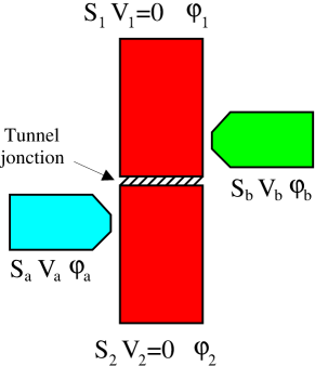
Figure 10: A four-terminal set-up of interest. The separation between the $S_{1}/S_{a}$ and $S_{2}/S_{b}$ contacts is comparable to the coherence length.

Appendix A Notations used for Green’s functions

A.1 Microscopic Green’s functions

The three superconducting electrodes $S_{a_{l}}$ ($a_{l}\in\{a,b,0\}$) are described by the BCS Hamiltonian:

$${\cal H}_{a_{l}} = -W\sum_{\langle i,j\rangle}\sum_{\sigma=\uparrow,\downarrow}\left(c_{i,\sigma}^{+}c_{j,\sigma}+h.c.\right))$$

$$- \sum_{i}\left(\Delta e^{i\varphi_{a_{l}}}c_{i,\uparrow}^{+}c_{i,\downarrow}^{+}+h.c.\right),$$

where $\langle i,j\rangle$ is a pair of nearest neighbors on a cubic lattice. The interfaces are coupled by an intermediate hopping amplitude:

$${\cal H}_{T,l}=-\Sigma_{0}\sum_{\langle a_{n},\alpha_{n}\rangle}\left(c_{a_{n},\sigma}^{+}c_{\alpha_{n},\sigma}+h.c.\right)).$$ (7)

The labels $a_{n}$ and $b_{m}$ in the Green’s functions correspond to the tight-binding sites at the interfaces of $S_{a}$ and $S_{b}$ respectively (see Fig. 2). The labels $\alpha_{n}$ and $\beta_{m}$ correspond to tight-binding sites in $S_{0}$, on both interfaces. The nonlocal bare Green’s functions denoted by $g_{\alpha,\beta}$ connect two generic tight-binding sites $\alpha$ and $\beta$ on the $S_{0}$ side of both interfaces, separated by a typical distance $R$ (see Fig. 2). The zero-energy Green’s function $g_{\alpha,\beta}$ decreases exponentially with $R$, over the zero-energy coherence length inverse proportional to the superconducting gap. Two additional labels associated to precisely which tight-binding site is concerned among all tight-binding sites present at the interface, have been made implicit in order to avoid heavy notations. The fully dressed Green’s functions are denoted by $G$. It is supposed in addition that the area of the multichannel contacts is much smaller than the squared coherence length.

The choice of the gauge is such that the phases at the origin of time are included in the superconducting Green’s function, and the transitions between harmonics of the Josephson frequency appear in the tunnel terms at the interfaces. The local Green’s functions take the same form for the three superconductors:

$$\hat{g}_{a_{l},a_{l}}^{A}(\omega)=\frac{1}{W\sqrt{(\Delta)^{2}-(\omega-i\eta)^{2}}}$$ (8)

$$\left(\begin{array}[]{cc}-(\omega-i\eta)&\Delta\exp(i\varphi_{a_{l}})\\ \Delta\exp(-i\varphi_{a_{l}})&-(\omega-i\eta)\end{array}\right),$$ (11)

where $a_{l}\in\{a,b\}$ labels each of the superconductors $S_{a}$ and $S_{b}$, and $a_{l}\in\{\alpha,\beta\}$ are tight-binding sites belong to $S_{0}$, on opposite interfaces. The three superconductors have the same gap $\Delta$. The phases at $t=0$ in $S_{a},S_{b}$ and $S_{0}$ are denoted by $\varphi_{a},\varphi_{b}$ and $\varphi_{0}$. The parameter $\eta$ can be viewed as a phenomenological linewidth broadening, introduced as an imaginary to the energy $\omega$. The parameter $\eta\ll\Delta$ takes a finite value in the numerical calculations where it plays the role of regularizing infinities in the partially resummed perturbative expansions.

The nonlocal Green’s function crossing $S_{0}$ takes the form

$$\hat{g}_{\alpha,\beta}^{A}(\omega)=\hat{g}_{\beta,\alpha}^{A}(\omega)=\frac{1}{W}\left\{\frac{\cos(k_{F}R)}{\sqrt{(\Delta)^{2}-(\omega-i\eta)^{2}}}\left(\begin{array}[]{cc}-(\omega-i\eta)&\Delta\exp(i\varphi_{0})\\ \Delta\exp(-i\varphi_{0})&-(\omega-i\eta)\end{array}\right)\right.+\left.\sin(k_{F}R)\left(\begin{array}[]{cc}1&0\\ 0&-1\end{array}\right)\right\}.$$ (16)

The retarded Green’s functions are obtained from the advanced Green’s functions by changing $\eta$ into $-\eta$.

A.2 Fourier transform of the Dyson-Keldysh equations

The Dyson equation in real time for the advanced Green’s function is given by the following convolution:

$$\hat{G}^{A}(t,t^{\prime}) = \hat{g}^{A}(t,t^{\prime})$$

$$+ \int dt_{1}\hat{g}^{A}(t,t_{1})\hat{\Sigma}(t_{1})\hat{G}^{A}(t_{1},t^{\prime}),$$

and a similar equation holds for the retarded Green’s function. The notation $\hat{\Sigma}(t)$ in Eq. (A.2) stands for a diagonal matrix encoding the time-dependent components of the Nambu hopping amplitudes. Similarly, the Keldysh Green’s function is given by

$$\hat{G}^{+,-}(t,t^{\prime})=\int dt_{1}dt_{2}\left(\hat{I}\delta(t-t_{1})+\hat{G}^{R}(t,t_{1})\hat{\Sigma}(t_{1})\right)$$ (18)

$$\times \hat{g}^{+,-}(t_{1},t_{2})\left(\hat{I}\delta(t_{2},t^{\prime})+\hat{\Sigma}(t_{2})\hat{G}^{A}(t_{2},t^{\prime})\right).$$

Terminal $S_{0}$ is grounded and terminals $S_{a}$ and $S_{b}$ are biased at voltages $V_{a}$ and $V_{b}$, with Josephson frequencies $\omega_{a}$ and $\omega_{b}$ respectively [with $\omega_{a,b}=2eV_{a,b}/\hbar$]. The two frequencies $\omega_{a,b}$ can be in an arbitrary ratio, commensurate or incommensurate.

A.3 Expression of the current

The current per channel between sites $a$ and $\alpha$ is the sum of four terms:

$$I_{a,\alpha}(t)=\frac{e}{h}\left[{\cal I}_{a,\alpha}^{1,1}(t)-{\cal I}_{\alpha,a}^{1,1}(t)-{\cal I}_{a,\alpha}^{2,2}(t)+{\cal I}_{\alpha,a}^{2,2}(t)\right],$$ (19)

with

$${\cal I}_{a,\alpha}^{1,1}(t) = \left[\hat{\Sigma}_{a,\alpha}(t)\hat{G}^{+,-}_{\alpha,a}(t,t)\right]^{1,1}$$ (20)

$${\cal I}_{\alpha,a}^{1,1}(t) = \left[\hat{\Sigma}_{\alpha,a}(t)\hat{G}^{+,-}_{a,\alpha}(t,t)\right]^{1,1}$$ (21)

$${\cal I}_{a,\alpha}^{2,2}(t) = \left[\hat{\Sigma}_{a,\alpha}(t)\hat{G}^{+,-}_{\alpha,a}(t,t)\right]^{2,2}$$ (22)

$${\cal I}_{\alpha,a}^{2,2}(t) = \left[\hat{\Sigma}_{\alpha,a}(t)\hat{G}^{+,-}_{a,\alpha}(t,t)\right]^{2,2},$$ (23)

where $G^{+,-}$ is the Keldysh Green’s function and $\hat{\Sigma}_{a,\alpha}(t)$ and $\hat{\Sigma}_{\alpha,a}(t)$ are the hopping amplitudes for transferring at time $t$ electrons or holes (according to the selected component of the $2\times 2$ matrix in Nambu) from $a$ to $\alpha$ or from $\alpha$ to $a$ respectively. The total current for the extended interface is the sum over all channels: $I(t)=\sum_{n}I_{a_{n},\alpha_{n}}(t)$.

Appendix B Symmetries of the current

B.1 Symmetry ${\cal S}_{1}$: checking that the current is a real number

The demonstration is illustrated on an example simpler than the full Keldysh Green’s function. Only one term contributing to the full $\hat{G}^{+,-}_{\alpha,a}$ is selected as an example:

$$\left[\hat{G}^{+,-}\right]_{\alpha,a}^{example} = \hat{g}^{A}_{\alpha,\beta}\hat{\Sigma}_{\beta,b}\hat{g}^{A}_{b,b}\hat{\Sigma}_{b,\beta}\hat{g}^{+,-}_{\beta,\alpha}\hat{\Sigma}_{\alpha,a}\hat{g}^{R}_{a,a}$$ (24)

$$\left[\hat{G}^{+,-}\right]_{a,\alpha}^{example} = \hat{g}^{A}_{a,a}\hat{\Sigma}_{a,\alpha}\hat{g}^{+,-}_{\alpha,\beta}\hat{\Sigma}_{\beta,b}\hat{g}^{R}_{b,b}\hat{\Sigma}_{b,\beta}\hat{g}^{R}_{\beta,\alpha}$$ (25)

Then, the following identities are deduced:

$$\left[\hat{\Sigma}_{a,\alpha}\left[\hat{G}^{+,-}\right]_{\alpha,a}^{example}\right]^{t}$$

$$=\left[\hat{\Sigma}_{a,\alpha}\hat{g}^{A}_{\alpha,\beta}\hat{\Sigma}_{\beta,b}\hat{g}^{A}_{b,b}\hat{\Sigma}_{b,\beta}\hat{g}^{+,-}_{\beta,\alpha}\hat{\Sigma}_{\alpha,a}\hat{g}^{R}_{a,a}\right]^{t}$$

$$= \left(\hat{g}^{R}_{a,a}\right)^{t}\hat{\Sigma}_{\alpha,a}\left(\hat{g}^{+,-}_{\beta,\alpha}\right)^{t}\hat{\Sigma}_{b,\beta}\left(\hat{g}^{A}_{b,b}\right)^{t}\hat{\Sigma}_{\beta,b}\left(\hat{g}^{A}_{\alpha,\beta}\right)^{t}\hat{\Sigma}_{a,\alpha}$$

$$= \left(\hat{g}^{A}_{a,a}\right)^{*}\hat{\Sigma}_{\alpha,a}\left(-\hat{g}^{+,-}_{\alpha,\beta}\right)^{*}\hat{\Sigma}_{b,\beta}\left(\hat{g}^{R}_{b,b}\right)^{*}\hat{\Sigma}_{\beta,b}\left(\hat{g}^{R}_{\beta,\alpha}\right)^{*}\hat{\Sigma}_{a,\alpha}$$

$$= -\left(\hat{g}^{A}_{a,a}\hat{\Sigma}_{a,\alpha}\hat{g}^{+,-}_{\alpha,\beta}\hat{\Sigma}_{\beta,b}\hat{g}^{R}_{b,b}\hat{\Sigma}_{b,\beta}\hat{g}^{R}_{\beta,\alpha}\hat{\Sigma}_{\alpha,a}\right)^{*}$$

$$= \left[\left[\hat{G}^{+,-}\right]_{a,\alpha}^{example}\hat{\Sigma}_{\alpha,a}\right]^{*},$$

where the following identity deduced from Eq. (16) were used:

$$\mbox{Symmetry ${\cal S}_{1}$: }(\hat{g}^{A})^{t}(\omega,\varphi)=(\hat{g}^{R})^{*}(\omega,\varphi).$$ (27)

Inserting the frequency variables leads to:

$$\left[\hat{\Sigma}_{a,\alpha}^{1,1}(\omega,\omega-\frac{\omega_{a}}{2})\left[\hat{G}^{+,-,11}\right]_{\alpha,a}^{example}(\omega-\frac{\omega_{a}}{2},\omega)\right]^{t}$$ (28)

$$=-\left[\left[\hat{G}^{+,-,1,1}\right]_{a,\alpha}^{example}(\omega,\omega-\frac{\omega_{a}}{2})\hat{\Sigma}_{\alpha,a}^{1,1}(\omega-\frac{\omega_{a}}{2},\omega)\right]^{*}..$$

It is deduced that

$$\left[\hat{\Sigma}_{a,\alpha}^{1,1}(\omega,\omega-\frac{\omega_{a}}{2})\left[\hat{G}^{+,-,11}\right]_{\alpha,a}(\omega-\frac{\omega_{a}}{2},\omega)\right]^{t}$$ (29)

$$=-\left[\left[\hat{G}^{+,-,1,1}\right]_{a,\alpha}(\omega,\omega-\frac{\omega_{a}}{2})\hat{\Sigma}_{\alpha,a}^{1,1}(\omega-\frac{\omega_{a}}{2},\omega)\right]^{*}..$$

Now, making a change of variable in the integral over $\omega$ leads to

$$\int d\omega\,\Sigma_{a}\left[\hat{G}^{+,-,t}\right]_{\alpha,a}^{1,1}(\omega-\frac{\omega_{a}}{2},\omega)$$

$$= -\int d\omega\,\Sigma_{a}\left[\hat{G}^{+,-,*}\right]_{a,\alpha}^{1,1}(\omega+\frac{\omega_{a}}{2},\omega).$$

The notation $\Sigma_{a}$ stands for the “11” component of the Nambu tunnel amplitude connecting $S_{a}$ and $S_{c}$. The components $I_{\alpha,a}^{1,1}$ and $I_{a,\alpha}^{1,1}$ are given by

$$I_{\alpha,a}^{1,1} = \int d\omega\left[\hat{\Sigma}_{\alpha,a}\hat{G}^{+,-}_{a,\alpha}\right]^{1,1}\left(\omega,\omega,\varphi_{a},\varphi_{b}\right)$$

$$= \int d\omega\,\Sigma_{a}\hat{G}^{+,-}_{a,\alpha}\left(\omega+\frac{\omega_{a}}{2},\omega,\varphi_{a},\varphi_{b},\varphi_{0}\right)$$

$$I_{a,\alpha}^{1,1} = \int d\omega\left[\hat{\Sigma}_{a,\alpha}\hat{G}^{+,-}_{\alpha,a}\right]^{1,1}\left(\omega,\omega,\varphi_{a},\varphi_{b}\right)$$

$$= \int d\omega\,\Sigma_{a}\hat{G}^{+,-}_{\alpha,a}\left(\omega-\frac{\omega_{a}}{2},\omega,\varphi_{a},\varphi_{b},\varphi_{0}\right).$$

It is concluded that $(I_{a,\alpha}^{1,1})=-(I_{\alpha,a}^{1,1})^{*}$, and $(I_{a,\alpha}^{2,2})=-(I_{\alpha,a}^{2,2})^{*}$, where the minus sign arises from the Keldysh Green’s function $g^{+,-}$.

B.2 Symmetry ${\cal S}_{2}$: changing the sign of the phases

The Green’s function given by Eq. (16) is antisymmetric under the following transformation:

$$\mbox{Symmetry ${\cal S}_{2}$: }g^{A}(\omega,\varphi)=-\left[\left[g^{A}(-\omega,\pi-\varphi)\right]^{*}\right]^{11\leftrightarrow 22}.$$ (33)

The symbol “$11\leftrightarrow 22$” means that the “11” and “22” Nambu components have been exchanged. A similar relation holds for the Nambu hopping amplitude matrix: $\hat{\Sigma}=-(\hat{\Sigma}^{*})^{11\leftrightarrow 22}$, for the fully dressed Green’s functions: $\hat{G}^{A}(\omega,\varphi)=-\left[\left[\hat{G}^{A}(-\omega,\pi-\varphi)\right]^{*}\right]^{11\leftrightarrow 22}$. The demonstration for the Keldysh Green’s function is as follows:

$$g^{+,-}(\omega,\varphi)=n_{F}(\omega)\left[g^{A}(\omega,\varphi)-g^{R}(\omega,\varphi)\right]$$ (34)

$$= \left[n_{F}(\omega)-n_{F}(-\omega)+n_{F}(-\omega)\right]\left[g^{A}(\omega,\varphi)-g^{R}(\omega,\varphi)\right]$$ (35)

$$= -n_{F}(-\omega)\left[\left(g^{A}(-\omega,\pi-\varphi)\right)^{*,11\leftrightarrow 22}-\left(g^{R}(-\omega,\pi-\varphi)\right)^{*,11\leftrightarrow 22}\right]+\left[n_{F}(\omega)-n_{F}(-\omega)\right]\left[g^{A}(\omega,\varphi)-g^{R}(\omega,\varphi)\right]$$ (36)

$$= -\left[g^{+,-}(-\omega,\pi-\varphi)\right]^{*,11\leftrightarrow 22}+\left[n_{F}(\omega)-n_{F}(-\omega)\right]\left[g^{A}(\omega,\varphi)-g^{R}(\omega,\varphi)\right].$$ (37)

One obtains the following:

$$\int d\omega\hat{\Sigma}_{a,\alpha}^{1,1}\left[\hat{G}^{+,-}\right]_{\alpha,a}^{1,1}(\omega,\omega,\varphi_{a},\varphi_{b},\varphi_{0})$$ (38)

$$= \int d\omega\,\hat{\Sigma}_{a}\left[\left(\hat{I}+\hat{G^{R}}\hat{\Sigma}\right)\hat{g}^{+,-}\left(\hat{I}+\hat{\Sigma}\hat{G}^{A}\right)\right]_{\alpha,a}^{1,1}(\omega+\frac{\omega_{a}}{2},\varphi_{a},\varphi_{b},\varphi_{0})$$ (39)

$$= -\int d\omega\,\Sigma_{a}\left\{\left[\left(\hat{I}+\hat{G^{R}}\hat{\Sigma}\right)\hat{g}^{+,-}\left(\hat{I}+\hat{\Sigma}\hat{G}^{A}\right)(-\omega-\frac{\omega_{a}}{2},-\omega,-\varphi_{a},-\varphi_{b},-\varphi_{0})\right]^{*,11\leftrightarrow 22}\right\}_{\alpha,a}^{1,1}$$

$$+\int d\omega\,\Sigma_{a}\left[\left(\hat{I}+\hat{G^{R}}\hat{\Sigma}\right)\delta\hat{g}^{+,-}\left(\hat{I}+\hat{\Sigma}\hat{G}^{A}\right)\right]_{\alpha,a}^{1,1}(\omega+\frac{\omega_{a}}{2},\omega,\varphi_{a},\varphi_{b},\varphi_{0})$$

$$= -\int d\omega\,\Sigma_{a}\left\{\left[\left(\hat{I}+\hat{G^{R}}\hat{\Sigma}\right)\hat{g}^{+,-}\left(\hat{I}+\hat{\Sigma}\hat{G}^{A}\right)\right](\omega-\frac{\omega_{a}}{2},\omega,-\varphi_{a},-\varphi_{b},-\varphi_{0})\right\}_{\alpha,a}^{*,2,2}$$

$$+\int d\omega\,\Sigma_{a}\left[\left(\hat{I}+\hat{G^{R}}\hat{\Sigma}\right)\delta\hat{g}^{+,-}\left(\hat{I}+\hat{\Sigma}\hat{G}^{A}\right)\right]_{\alpha,a}^{1,1}(\omega+\frac{\omega_{a}}{2},\omega,\varphi_{a},\varphi_{b},\varphi_{0}),$$

where

$$g^{+,-}(\omega,\varphi) = -\left[g^{+,-}(-\omega,\pi-\varphi)\right]^{*,11\leftrightarrow 22}+\delta g^{+,-}(\omega,\varphi)$$ (42)

$$\delta g^{+,-}(\omega,\varphi) = \left[n_{F}(\omega)-n_{F}(-\omega)\right]\left[g^{A}(\omega,\varphi)-g^{R}(\omega,\varphi)\right].$$ (43)

The following identity was used in order to obtain Eq. (42):

$$g^{+,-}(\omega,\varphi) = \left[n_{F}(\omega)-n_{F}(-\omega)\right]\left[g^{A}(\omega,\varphi)-g^{R}(\omega,\varphi)\right]+n_{F}(-\omega)\left[g^{A}(\omega,\varphi)-g^{R}(\omega,\varphi)\right]$$ (44)

Thus, the total current is given by

$$I_{tot}(eV_{a},eV_{b},\varphi_{a},\varphi_{b},\varphi_{0})=2\Re\left[I_{a,\alpha}^{2,2}(eV_{a},eV_{b},\varphi_{a},\varphi_{b},\varphi_{0})-I_{a,\alpha}^{2,2}(eV_{a},eV_{b},-\varphi_{a},-\varphi_{b},-\varphi_{0})\right]$$ (45)

$$+ 2\Re\left[\int d\omega\hat{\Sigma}_{a,\alpha}^{1,1}\left[\left(\hat{I}+\hat{G}^{R}\hat{\Sigma}\right)\delta\hat{g}^{+,-}\left(\hat{I}+\hat{\Sigma}\hat{G}^{A}\right)\right]^{1,1}_{\alpha,a}(\omega+\frac{\omega_{a}}{2},\omega,\varphi_{a},\varphi_{b},\varphi_{0})\right].$$

Appendix C Sketch of the analytical calculations

C.1 Expansion of the Green’s functions in the number of nonlocal bare Green’s functions

Now, the approximations are presented. The starting point is the Dyson equations for the fully dressed Green’s functions $\hat{G}$ which take the form

$$\hat{G}_{\beta,\beta} = \hat{g}_{\beta,\beta}+\hat{G}_{\beta,\alpha}\hat{\Sigma}_{\alpha,a}\hat{g}_{a,a}\hat{\Sigma}_{a,\alpha}\hat{g}_{\alpha,\beta}$$

$$+ \hat{G}_{\beta,\beta}\hat{\Sigma}_{\beta,b}\hat{g}_{b,b}\hat{\Sigma}_{b,\beta}\hat{g}_{\beta,\beta}$$

$$\hat{G}_{\alpha,\beta} = \hat{g}_{\alpha,\beta}+\hat{g}_{\alpha,\alpha}\hat{\Sigma}_{\alpha,a}\hat{g}_{a,a}\hat{\Sigma}_{a,\alpha}\hat{G}_{\alpha,\beta}$$

$$+ \hat{g}_{\alpha,\beta}\hat{\Sigma}_{\beta,b}\hat{g}_{b,b}\hat{\Sigma}_{b,\beta}\hat{G}_{\beta,\beta}.$$

Those Dyson equations are next expanded in the number of nonlocal bare Green’s functions. The expression of the Green’s functions to order $(g_{\alpha,\beta})^{2}$ is the following:

$$\hat{G}_{\alpha,\beta} = \hat{A}^{(\alpha,\beta)}_{a}\hat{g}_{\alpha,\beta}\hat{B}^{(\alpha,\beta)}_{b}+{\cal O}\left(g_{\alpha,\beta}\right)^{3}$$ (48)

$$\hat{G}_{\beta,\beta} = \hat{A}^{(\beta,\beta)}_{a}+\hat{B}^{(\beta,\beta)}_{b}\hat{g}_{\beta,\alpha}\hat{C}^{(\beta,\beta)}_{a}\hat{g}_{\alpha,\beta}\hat{D}^{(\beta,\beta)}_{b}$$

$$+ {\cal O}\left(g_{\alpha,\beta}\right)^{4},$$

with

$$\hat{A}^{(\alpha,\beta)}_{a} = \left[\hat{I}-\hat{g}_{\alpha,\alpha}\hat{\Sigma}_{\alpha,a}\hat{g}_{a,a}\hat{\Sigma}_{a,\alpha}\right]^{-1}$$ (50)

$$\hat{B}^{(\alpha,\beta)}_{b} = \left[\hat{I}-\hat{\Sigma}_{\beta,b}\hat{g}_{b,b}\hat{\Sigma}_{b,\beta}\hat{g}_{\beta,\beta}\right]^{-1}$$ (51)

$$\hat{A}^{(\beta,\beta)}_{b} = \left[\hat{I}-\hat{g}_{\beta,\beta}\hat{\Sigma}_{\beta,b}\hat{g}_{b,b}\hat{\Sigma}_{b,\beta}\right]^{-1}\hat{g}_{\beta,\beta}$$ (52)

$$\hat{B}^{(\beta,\beta)}_{b} = \left[\hat{I}-\hat{g}_{\beta,\beta}\hat{\Sigma}_{\beta,b}\hat{g}_{b,b}\hat{\Sigma}_{b,\beta}\right]^{-1}$$ (53)

$$\hat{C}^{(\beta,\beta)}_{a} = \hat{\Sigma}_{\alpha,a}\hat{g}_{a,a}\hat{\Sigma}_{a,\alpha}\left[\hat{I}-\hat{g}_{\alpha,\alpha}\hat{\Sigma}_{\alpha,a}\hat{g}_{a,a}\hat{\Sigma}_{a,\alpha}\right]^{-1}$$ (54)

$$\hat{D}^{(\beta,\beta)}_{b} = \left[\hat{I}-\hat{\Sigma}_{\beta,b}\hat{g}_{b,b}\hat{\Sigma}_{b,\beta}\hat{g}_{\beta,\beta}\right]^{-1},$$ (55)

where the superscript refers to the overall propagation in the fully dressed Green’s function, and the subscript a or b refers to processes taking place “locally” within each $S_{a}S_{0}$ or $S_{b}S_{0}$ interface. Similar expressions are obtained for $\hat{G}_{\beta,\alpha}$ and $\hat{G}_{\alpha,\alpha}$.

C.2 Exact expression of the fully dressed Keldysh Green’s function

Appendix C.1 above deals with the expansion of the advanced and retarded Green’s functions. Now, the same expansion is carried out for the Keldysh Green’s function. The first step is to obtain the specific expression of the Keldysh Green’s function for the three-terminal structure under consideration. The exact fully dressed Keldysh Green’s function is obtained as the sum of 12 terms:

$$\hat{\Sigma}_{\alpha,a}\hat{G}^{+,-}_{a,\alpha}=$$

$$\hat{F}_{1}\left[\hat{\Sigma}_{\alpha,a}\hat{g}^{+,-}_{a,a}\hat{\Sigma}_{a,\alpha}\right]$$

$$+ \hat{F}_{2}\left[\hat{\Sigma}_{\alpha,a}\hat{g}^{R}_{a,a}\hat{\Sigma}_{a,\alpha}\left|\right.\hat{\Sigma}_{\alpha,a}\hat{g}^{+,-}_{a,a}\hat{\Sigma}_{a,\alpha}\right]$$

$$+ \hat{F}_{3}\left[\hat{\Sigma}_{\alpha,a}\hat{g}^{R}_{a,a}\hat{\Sigma}_{a,\alpha}\left|\right.\hat{\Sigma}_{\beta,b}\hat{g}^{+,-}_{b,b}\hat{\Sigma}_{b,\beta}\right]$$

$$+ \hat{F}_{4}\left[\hat{\Sigma}_{\alpha,a}\hat{g}^{R}_{a,a}\hat{\Sigma}_{a,\alpha}\hat{g}^{+,-}_{\alpha,\alpha}\right]$$

$$+ \hat{F}_{5}\left[\hat{\Sigma}_{\alpha,a}\hat{g}^{R}_{a,a}\hat{\Sigma}_{a,\alpha}\left|\right.\hat{\Sigma}_{\alpha,a}\hat{g}^{R}_{a,a}\hat{\Sigma}_{a,\alpha}\hat{g}^{+,-}_{\alpha,\alpha}\right]$$

$$+ \hat{F}_{1}\left[\hat{\Sigma}_{\alpha,a}\hat{g}^{R}_{a,a}\hat{\Sigma}_{a,\alpha}\hat{g}^{+,-}_{\alpha,\alpha}\hat{\Sigma}_{\alpha,a}\hat{g}^{A}_{a,a}\hat{\Sigma}_{a,\alpha}\right]$$

$$+ \hat{F}_{2}\left[\hat{\Sigma}_{\alpha,a}\hat{g}^{R}_{a,a}\hat{\Sigma}_{a,\alpha}\left|\right.\hat{\Sigma}_{\alpha,a}\hat{g}^{R}_{a,a}\hat{\Sigma}_{a,\alpha}\hat{g}^{+,-}_{\alpha,\alpha}\hat{\Sigma}_{\alpha,a}\hat{g}^{A}_{a,a}\hat{\Sigma}_{a,\alpha}\right]$$

$$+ \hat{F}_{3}\left[\hat{\Sigma}_{\alpha,a}\hat{g}^{R}_{a,a}\hat{\Sigma}_{a,\alpha}\left|\right.\hat{\Sigma}_{\beta,b}\hat{g}^{R}_{b,b}\hat{\Sigma}_{b,\beta}\hat{g}^{+,-}_{\beta,\beta}\hat{\Sigma}_{\beta,b}\hat{g}^{A}_{b,b}\hat{\Sigma}_{b,\beta}\right]$$

$$+ F_{6}\left[\hat{\Sigma}_{\alpha,a}\hat{g}^{R}_{a,a}\hat{\Sigma}_{a,\alpha}\left|\right.\hat{\Sigma}_{\beta,b}\hat{g}^{A}_{b,b}\hat{\Sigma}_{b,\beta}\right]$$

$$+ \hat{F}_{7}\left[\hat{\Sigma}_{\alpha,a}\hat{g}^{R}_{a,a}\hat{\Sigma}_{a,\alpha}\left|\right.\hat{\Sigma}_{\alpha,a}\hat{g}^{R}_{a,a}\hat{\Sigma}_{a,\alpha}\left|\right.\hat{\Sigma}_{\beta,b}\hat{g}^{A}_{b,b}\hat{\Sigma}_{b,\beta}\right]$$

$$+ \hat{F}_{8}\left[\hat{\Sigma}_{\alpha,a}\hat{g}^{R}_{a,a}\hat{\Sigma}_{a,\alpha}\left|\right.\hat{\Sigma}_{\beta,b}\hat{g}^{R}_{b,b}\hat{\Sigma}_{b,\beta}\right]$$

$$+ \hat{F}_{9}\left[\hat{\Sigma}_{\alpha,a}\hat{g}^{R}_{a,a}\hat{\Sigma}_{a,\alpha}\left|\right.\hat{\Sigma}_{\beta,b}\hat{g}^{R}_{b,b}\hat{\Sigma}_{b,\beta}\left|\right.\hat{\Sigma}_{\alpha,a}\hat{g}^{A}_{a,a}\hat{\Sigma}_{a,\alpha}\right],$$

with

$$\hat{F}_{1}\left[\hat{X}\right] = \hat{X}\hat{G}_{\alpha,\alpha}^{A}$$ (57)

$$\hat{F}_{2}\left[\hat{X}\left|\right.\hat{Y}\right] = \hat{X}\hat{G}_{\alpha,\alpha}^{R}\hat{Y}\hat{G}^{A}_{\alpha,\alpha}$$ (58)

$$\hat{F}_{3}\left[\hat{X}\left|\right.\hat{Y}\right] = \hat{X}\hat{G}_{\alpha,\beta}^{R}\hat{Y}\hat{G}^{A}_{\beta,\alpha}$$ (59)

$$\hat{F}_{4}\left[\hat{X}\right] = \hat{X}$$ (60)

$$\hat{F}_{5}\left[\hat{X}\left|\right.\hat{Y}\right] = \hat{X}\hat{G}^{R}_{\alpha,\alpha}\hat{Y}$$ (61)

$$\hat{F}_{6}\left[\hat{X}\left|\right.\hat{Y}\right] = \hat{X}\hat{g}^{+,-}_{\alpha,\beta}\hat{Y}\hat{G}^{A}_{\beta,\alpha}$$ (62)

$$\hat{F}_{7}\left[\hat{X}\left|\right.\hat{Y}\left|\right.\hat{Z}\right] = \hat{X}\hat{G}^{R}_{\alpha,\alpha}\hat{Y}\hat{g}^{+,-}_{\alpha,\beta}\hat{Z}\hat{G}^{A}_{\beta,\alpha}$$ (63)

$$\hat{F}_{8}\left[\hat{X}\left|\right.\hat{Y}\right] = \hat{X}\hat{G}^{R}_{\alpha,\beta}\hat{Y}\hat{g}^{+,-}_{\beta,\alpha}$$ (64)

$$\hat{F}_{9}\left[\hat{X}\left|\right.\hat{Y}\left|\right.\hat{Z}\right] = \hat{X}\hat{G}^{R}_{\alpha,\beta}\hat{Y}\hat{g}^{+,-}_{\beta,\alpha}\hat{Z}\hat{G}^{A}_{\alpha,\alpha},$$ (65)

where the matrices $\hat{X}$, $\hat{Y}$ and $\hat{Z}$ do not couple the two interfaces.

C.3 Expansion of the Keldysh Green’s function in the number of nonlocal bare Green’s functions

In the next step, all of the fully dressed advanced and retarded Green’s functions in $\hat{F}_{n}$ ($n=1...9$) are expanded in perturbation in the number of nonlocal bare Green’s function. The final expression of the Keldysh Green’s functions first involves the matrix elements of some products between the matrices $\hat{X}$, $\hat{Y}$ and $\hat{Z}$, and the matrices $\hat{A}$, $\hat{B}$, $\hat{C}$ and $\hat{D}$. Each of the bare nonlocal bare Green’s functions

$$\langle\langle\hat{g}_{\alpha,\beta}\left(\alpha^{1},N_{a}^{1}\left|\right.\alpha^{2},N_{b}^{2}\right)\hat{g}_{\beta,\alpha}\left(\alpha^{3},N_{b}^{3}\left|\right.\alpha^{4},N_{a}^{4}\right)\rangle\rangle$$ (66)

is evaluated from Fourier transform over times $t$ and $t^{\prime}$:

$$\hat{g}_{\alpha,\beta}\left(\alpha^{1},N_{a}^{1}\left|\right.\alpha^{2},N_{b}^{2}\right)$$

$$= \int dtdt^{\prime}\exp{\left\{i\left[\omega+N_{a}^{1}\frac{\omega_{a}}{2}\right]t\right\}}$$

$$\times \exp{\left\{-i\left[\omega+N_{b}^{2}\frac{\omega_{b}}{2}\right]t^{\prime}\right\}}\hat{g}_{\alpha,\beta}(t^{\prime}-t)$$

$$= \delta_{\left[N_{a}^{1}\frac{\omega_{a}}{2}\right]-\left[N_{b}^{2}\frac{\omega_{b}}{2}\right]}\hat{g}_{\alpha,\beta}\left(\omega+N_{a}^{1}\frac{\omega_{a}}{2}\right),$$ (68)

where $\alpha^{n}$ is a Nambu label. The quantities $N_{a}^{1}$ and $N_{b}^{2}$ encodes multiples of the voltage frequencies $\omega_{a}/2\equiv eV_{a}$ and $\omega_{b}/2\equiv eV_{b}$ in electrodes $S_{0}S_{a}$ and $S_{0}S_{b}$. Eq. (68) is valid for arbitrary values of $\omega_{a}$ and $\omega_{b}$, not necessarily commensurate.

œ Coming back to the expansion of the Keldysh function at the lowest order-two, an example is the following:

$$\hat{F}_{2}\left[\hat{X}\left.\right|\hat{Y}\right] = \hat{X}\hat{A}^{(\alpha,\alpha),R}\hat{Y}\hat{A}^{(\alpha,\alpha),A}+\hat{X}\hat{A}^{(\alpha,\alpha),R}\hat{Y}\hat{B}^{(\alpha,\alpha),A}\hat{g}_{\alpha,\beta}^{A}\hat{C}^{(\alpha,\alpha),A}\hat{g}_{\beta,\alpha}^{A}\hat{D}^{(\alpha,\alpha),A}$$

$$+ \hat{X}\hat{B}^{(\alpha,\alpha),R}\hat{g}_{\alpha,\beta}^{R}\hat{C}^{(\alpha,\alpha),R}\hat{g}_{\beta,\alpha}^{R}\hat{D}^{(\alpha,\alpha),R}\hat{Y}\hat{A}^{(\alpha,\alpha),A}+{\cal O}\left((g_{\alpha,\beta})^{4}\right).$$

Expanding all matrix products leads to

$$\left\{\hat{F}_{2}\left[\hat{X}\left.\right|\hat{Y}\right]\right\}_{0,0}=\left\{\hat{X}\hat{A}^{(\alpha,\alpha),R}\hat{Y}\hat{A}^{(\alpha,\alpha),A}\right\}_{0,0}$$

$$+ \sum_{\kappa_{1},\kappa_{2},\kappa_{3}}\left\{\hat{X}\hat{A}^{(\alpha,\alpha),R}\hat{Y}\hat{B}^{(\alpha,\alpha),A}\right\}_{0,\kappa_{1}}\times\left\{\hat{C}^{(\alpha,\alpha),A}\right\}_{\kappa_{2},\kappa_{3}}\left\{\hat{D}^{(\alpha,\alpha),A}\right\}_{\kappa_{4},0}\langle\langle\left\{\hat{g}_{\alpha,\beta}^{A}\right\}_{\kappa 1,\kappa 2}\left\{\hat{g}_{\beta,\alpha}^{A}\right\}_{\kappa_{3},\kappa_{4}}\rangle\rangle$$

$$+ \sum_{\kappa_{1},\kappa_{2},\kappa_{3}}\left\{\hat{X}\hat{B}^{(\alpha,\alpha),R}\right\}_{0,\kappa_{1}}\left\{\hat{C}^{(\alpha,\alpha),R}\right\}_{\kappa_{2},\kappa_{3}}\left\{\hat{D}^{(\alpha,\alpha),R}\hat{Y}\hat{A}^{(\alpha,\alpha),A}\right\}_{\kappa_{4},0}\langle\langle\left\{\hat{g}_{\alpha,\beta}^{R}\right\}_{\kappa_{1},\kappa_{2}}\left\{\hat{g}_{\beta,\alpha}^{R}\right\}_{\kappa_{3},\kappa_{4}}\rangle\rangle$$

$$+ {\cal O}\left((g_{\alpha,\beta})^{4}\right).$$

The variables $\kappa_{n}$ (with $n=1,2,3$) label both Nambu and the harmonics of the Josephson frequency. The average over the Friedel oscillations in Eq. (66) may appear as a standard procedure within the theory of nonlocal transport in three-terminal $NSN$ structures Falci ; Melin-Feinberg ; Melin-Feinberg-EPJB :

$$\langle\langle F\rangle\rangle(R)=\frac{k_{F}}{2\pi}\int_{R-\pi/k_{F}}^{R+\pi/k_{F}}F(r)dr,$$ (71)

where the function $F(r)$ has rapid Friedel oscillations at the scale of the Fermi wavelength $\lambda_{F}=2\pi/k_{F}$ (to be averaged out because of multichannel averaging), but its envelope decays smoothly on the much longer scale of the coherence length $\xi$. The Nambu elements of the non-local Green’s function $\hat{g}_{\alpha,\beta}^{\epsilon_{1}}(R)$ can be written as

$$\hat{g}_{\alpha,\beta}^{\epsilon_{1}}(R)=\frac{f(R)}{W}\exp\left\{-\frac{R}{\xi\left(\omega-i\eta\epsilon_{1}\right)}\right\}\left\{\frac{\cos{(k_{F}R)}}{\sqrt{\Delta^{2}-(\omega-i\eta\epsilon_{1})^{2}}}\left[\begin{array}[]{cc}-(\omega-i\eta\epsilon_{1})&\Delta\\ \Delta&-(\omega-i\eta\epsilon_{1})\end{array}\right]\right.$$ (74)

$$\left.+\sin(k_{F}R)\left[\begin{array}[]{cc}1&0\\ 0&-1\end{array}\right]\right\},$$ (77)

where $\epsilon_{1}=\pm$ labels advanced or retarded. The exponent in its power-law decay is dimension-dependent, and $\xi(\omega)$ is the energy-dependent coherence length. The parameter $\eta$ is a small linewidth broadening. The function $f(R)$ is a prefactor that does not oscillate at the scale of the Fermi wave-length. It will be taken as a constant in our numerical calculations, because the contacts are at distance large compared to their size.

Using $\langle\langle\cos^{2}(k_{F}R)\rangle\rangle=\langle\langle\sin^{2}(k_{F}R)\rangle\rangle=1/2$ and $\langle\langle\cos(k_{F}R)\sin(k_{F}R)\rangle\rangle=0$ leads to

$$\langle\langle\hat{g}_{\alpha,\beta}^{\epsilon_{1}}\otimes\hat{g}_{\beta,\alpha}^{\epsilon_{2}}\rangle\rangle=\frac{1}{2}\left(\frac{f(R)}{W}\right)^{2}\exp\left\{-\frac{R}{\xi(\omega-i\eta\epsilon_{1})}\right\}\exp\left\{-\frac{R}{\xi(\omega-i\eta\epsilon_{2})}\right\}$$ (78)

$$\times \left\{h_{\epsilon_{1},\epsilon_{2}}(\omega_{0},\tilde{\omega}_{0})\left[\begin{array}[]{cc}-(\omega_{0}-i\eta\epsilon_{1})&\Delta\\ \Delta&-(\omega_{0}-i\eta\epsilon_{1})\end{array}\right]_{\rm Nambu}\otimes\left[\begin{array}[]{cc}-(\tilde{\omega}_{0}-i\eta\epsilon_{2})&\Delta\\ \Delta&-(\tilde{\omega}_{0}-i\eta\epsilon_{2})\end{array}\right]_{\rm Nambu}\right.$$ (88)

$$+\left.\left[\begin{array}[]{cc}1&0\\ 0&-1\end{array}\right]_{\rm Nambu}\otimes\left[\begin{array}[]{cc}1&0\\ 0&-1\end{array}\right]_{\rm Nambu}\right\},$$

with

$$h_{\epsilon_{1},\epsilon_{2}}(\omega_{0},\tilde{\omega}_{0})=\frac{1}{\sqrt{\Delta^{2}-(\omega_{0}-i\eta\epsilon_{1})^{2}}\sqrt{\Delta^{2}-(\tilde{\omega}_{0}-i\eta\epsilon_{2})^{2}}},$$ (89)

with

$$N_{a}^{1}\omega_{a} = N_{b}^{2}\omega_{b}$$ (90)

$$N_{b}^{3}\omega_{b} = N_{a}^{4}\omega_{a}$$ (91)

and with $\omega_{0}=\omega+N_{a}^{1}\omega_{a}/2$ and $\tilde{\omega}_{0}=\omega+N_{b}^{3}\omega_{b}$.

Appendix D Details on the numerics

The expansion in the number of nonlocal bare Green’s functions sketched in the previous Appendices was combined to an algorithm for evaluating the local Green’s functions dressed by processes taking place “locally” at each $S_{a}S_{0}$ or $S_{b}S_{0}$ interface. All components of the Green’s functions connecting any harmonics to any other are required to be evaluated in order to obtain the fully dressed Keldysh Green’s function of the three-terminal $S_{a}S_{0}S_{b}$ structure, approximated as above . However, inversions of matrices connecting both interfaces are never required to be performed, which explains the reduced computation times. Direct matrix inversion of matrices defined locally at a single interface and thus not coupling the two interfaces is numerically efficient if the cut-off in the number of harmonics of the Josephson frequency is not larger than $\sim 10$, which is the case in what follows because the calculations are restricted to voltage $eV\gtrsim\Delta/10$. Otherwise, if needed, a possible future version of the code will evaluate the fully dressed local Green’s functions from one-dimensional recursive Green’s functions in energy Cuevas , allowing for the possibility of addressing voltages smaller than $eV\lesssim\Delta/10$.

The size of the matrices to be inverted would be

$$[2(2N_{max}+1)^{2}]\times[2(2N_{max}+1)^{2}],$$ (92)

if all information about nonlocal processes would be kept in a frontal approach. Programming the problem in this way was attempted, but running codes with increasing values of $N_{max}$ upon reducing voltage becomes undoable with standard computer resources, even if the voltages are not necessarily small compared to the gap. In addition, the prohibitive computation time given by Eq. (92) has to be multiplied by a factor $N_{k_{F}R}$, in order to calculate the integral over the Friedel oscillations with microscopic phase factor $k_{F}R$ suitable for a multichannel contact (see Eq. 71). Alternatively, the spatial aspect of this problem may be treated with recursive Green’s functions in real space, extended to include the harmonics of half the Josephson frequency (below a given voltage-sensitive cut-off), but this numerical implementation appears to be even more computationally demanding than an average over $k_{F}R$ for a collection of independent channels. A scaling factor in the computation time, of typical value $N_{\omega}={\cal O}(10^{3})$, is also required for the evaluation of the integral over energy of the spectral current (containing sharp resonances) with an adaptative algorithm.

The size of the matrices to be inverted with partially resummed perturbation theory used here is only

$$[2(2N_{max}+1)]\times[2(2N_{max}+1)],$$ (93)

not larger than for a single interface. In addition, the average over the Friedel oscillations is built-in in the case of the expansion in the number of nonlocal bare Green’s functions, and there is thus a gain of computation time by the factor $N_{k_{F}R}$, because, at the lowest order-two in the partially resummed perturbation theory, the multichannel junction maps onto a single-channel problem. Again, $N_{\omega}={\cal O}(10^{3})$ calls to the spectral current routine are required in order to integrate it over energy with an adaptative algorithm. Then, the numerical calculations become approximate, but, above all, they become doable without running them on a supercomputer.

References

- (1) J. C. Cuevas and H. Pothier, Phys. Rev. B 75, 174513 (2007).
- (2) N. A. H. Nerenberg, J. A. Blackburn, and D. W. Jillie, Phys. Rev. B 21, 118 (1980).
- (3) A. Freyn, B. Doucot, D. Feinberg, and R. Mélin, Phys. Rev. Lett. 106, 257005 (2011).
- (4) T. Jonckheere, J. Rech, T. Martin, B. Douçot, D. Feinberg, R. Mélin, Phys. Rev. B 87, 214501 (2013).
- (5) M. Houzet and P. Samuelsson, Phys. Rev. B 82, 06051 (2010).
- (6) B. van Heck, S. Mi, and A.R. Akhmerov, Phys. Rev. B 90, 155450 (2014).
- (7) D. Feinberg, T. Jonckheere, J. Rech, T. Martin, B. Douçot, and R. Mélin, Eur. Phys. J. B 88, 99 (2015).
- (8) C. Padurariu, T. Jonckheere, J. Rech, R. Mélin, D. Feinberg, T. Martin, Yu. V. Nazarov, Phys. Rev. B 92, 205409 (2015).
- (9) R.-P. Riwar, M. Houzet, J.S. Meyer, Y.V. Nazarov, arXiv:1503.06862
- (10) A.H. Pfeffer, J.E. Duvauchelle, H. Courtois, R. Mélin, D. Feinberg, F. Lefloch, Phys. Rev. B 90, 075401 (2014).
- (11) J.E. Duvauchelle et al., in preparation (2016).
- (12) M. Heiblum, private communication.
- (13) C. Padurariu, T. Jonckheere, J. Rech, T. Martin, R. Mélin, and D. Feinberg, in preparation (2016).
- (14) J. C. Cuevas, A. Martín-Rodero, and A. Levy Yeyati, Phys. Rev. B54, 7366 (1996).
- (15) J.C. Cuevas, J. Heurich, A. Martín-Rodero, A. Levy Yeyati and G. Schön, Phys. Rev. Lett. 88, 157001 (2002).
- (16) R. Mélin and D. Feinberg, Phys. Rev. B 70, 174509 (2004).
- (17) G.E. Blonder, M. Tinkham and T.M. Klapwijk, Phys. Rev. B 25, 4515 (1982).
- (18) R. Mélin, F.S. Bergeret, A. Levy Yeyati, Phys. Rev. B 79, 104518 (2009).
- (19) R. Mélin and D. Feinberg, Eur. Phys. J. B 26, 101 (2002).
- (20) G. Falci, D. Feinberg, and F. W. J. Hekking, Europhys. Lett. 54, 255 (2001).
- (21) D. Beckmann, H. B. Weber, and H. v. Löhneysen, Phys. Rev. Lett. 93, 197003 (2004)
- (22) S. Russo, M. Kroug, T. M. Klapwijk, and A. F. Morpurgo, Phys. Rev. Lett. 95, 027002 (2005).
- (23) P. Cadden-Zimansky and V. Chandrasekhar, Phys. Rev. Lett. 97, 237003 (2006); P. Cadden-Zimansky, Z. Ziang, and V. Chandrasekhar, New J. Phys. 9, 116 (2007).
- (24) S. Duhot, F. Lefloch, M. Houzet, Phys. Rev. Lett. 102, 086804 (2009).
- (25) C. Caroli, R. Combescot, P. Nozières, and D. Saint-James, J. Phys. C 4, 916 (1971); 5, 21 (1972).