Transverse-momentum-dependent quark splitting functions in $k_{T}$-factorization: real contributions

Abstract

We calculate transverse momentum dependent quark splitting kernels $P_{gq}$ and $P_{qq}$ within $k_{T}$-factorization, completing earlier results which concentrated on gluon splitting functions $P_{gg}$ and $P_{qg}$. The complete set of splitting kernels is an essential requirement for the formulation of a complete set of evolution equations for transverse momentum dependent parton distribution functions and the development of corresponding parton shower algorithms.

1 Introduction

The essential theoretical input for experimental findings at the Large Hadron Collider are parton distribution functions (PDFs) which describe momentum distributions of partons in the colliding hadrons in the presence of a hard scale. Together with factorization theorems and hard coefficient functions, PDFs allow to predict new phenomena and to describe existing data. A lot of recent activity in theory and phenomenology of QCD is devoted to so called transverse-momentum-dependent parton distribution functions (TMD PDFs) and TMD factorization (for a review we refer the Reader to Angeles-Martinez:2015sea ). While a rigorous formulation of TMD factorization, valid for all kinematic regions, is still to be achieved (see e.g. Col11 ), a definition of TMD parton distributions is possible for specific regions of phase space, usually characterized by a hierarchy of scales Balitsky:2015qba ; Dominguez:2011wm ; Kotko:2015ura ; Kovchegov:2015zha . One of those regions is the high-energy or small-$x$ limit of perturbative QCD, characterized by the hierarchy $\sqrt{s}\gg M\gg\Lambda_{\text{QCD}}$, where $\sqrt{s}$ denotes the center-of-mass energy of the process, $M$ the hard scale of the perturbative event, and $\Lambda_{\text{QCD}}$ the QCD characteristic scale of the order of a few hundred MeV. The underlying theoretical framework for TMD PDFs in this kinematic limit is usually referred to as $k_{T}$-factorization or high-energy factorization Catani:1990eg . During the recent years various hard processes, in particular those associated with the forward region of LHC detectors, characterized by large rapidities, have been studied within the $k_{T}$-factorization framework, such as forward jet and forward $b$-jet production Deak:2011ga ; Deak:2010gk ; Chachamis:2015ona and forward $Z$-production Dooling:2014kia ; Hautmann:2012sh ; vanHameren:2015uia .

In the following we are in particular interested in the evolution of TMD PDFs, which depends on the parton’s longitudinal momentum fraction $x$, its transverse momentum $k_{T}$, and the external hard scale $M$. An evolution equation which has these elements and is valid in angular ordered phase space for gluon emission is provided by the Ciafaloni-Catani-Fiorani-Marchesini (CCFM) equation Cia87 ; Marchesini:1994wr ; CFM90a ; CFM90b . The key element of the evolution kernel of the CCFM equation is the $P_{gg}$ splitting function. At leading order it contains only the most singular pieces at low $z\to 0$ and large $z\to 1$ and appropriate form factors which resum virtual and unresolved real emissions in respectively low and large $z$ regions.

The CCFM equation is restricted to the resummation of purely gluonic emissions. In particular this implies that the large-$x$ behavior of CCFM is not accurate and the formal large-$z$ limit of the CCFM equation is incomplete, since it does not reduce to the matrix-valued DGLAP evolution equations. One of the observations based on the Monte-Carlo implementation Jung:2010si of the CCFM equation is that the lack of such contributions leads indeed to non-negligible effects. Performing a fit to the proton structure function $F_{2}$ at both large and small $x$, it is likely that the gluon contribution is enhanced in regions where quarks in the evolution would contribute. While for inclusive observables, such as the structure function $F_{2}$, the overall fit turns out to be satisfactory, see e.g. Hautmann:2013tba , the predictions based on the gluon density are not satisfactory for exclusive observables, see e.g. Deak:2010gk . While it is difficult to pinpoint the exact reason for this deficiency, DGLAP resummation definitely suggests that decoupled evolution of quarks and gluons is insufficient. This is further supported by application of the Kutak-Sapeta (KS) gluons densities Kutak:2012rf ; Kutak:2014wga which account for quark contribution in the evolution Kwiecinski:1997ee and describes production of dijets in p+p collisions at LHC reasonably well Kutak:2012rf ; vanHameren:2014ala . In order to be able to apply CCFM evolution successfully and to provide full parton shower Monte-Carlo description within CCFM, the ultimate goal must be therefore to arrive at a coupled system of equations which in turn requires a full set of $k_{T}$-dependent splitting functions Jung:REF .

To arrive at a complete and consistent set of evolution equations, it is further necessary to include — apart from the quark splitting functions $P_{gq}$ and $P_{qq}$ — non-singular terms of the $P_{gg}$ splitting function since these corrections are of the same order beyond leading order (LO) CCFM, i.e. beyond large- and small-$z$ enhanced contributions. Note that in Jung:2010si it has been observed that inclusion of non-singular pieces of the DGLAP gluon splitting function into CCFM evolution strongly affects the solution of the evolution equation. One may therefore conclude that the effect of quarks in the evolution will be similarly significant.

A first step into this direction has undertaken in Hautmann:2012sh , where the TMD gluon-to-quark splitting kernel $P_{qg}$ obtained in CH94 has been used to define a TMD sea-quark density within $k_{T}$-factorization. In the following we extend this result by calculating as a start the unintegrated real emissions kernels for quark-to-quark and quark-to-gluon splitting functions.

From a technical point of view the determination of TMD splitting kernels is based on a generalization of the high energy factorization approach of Catani and Hautmann CH94 , which itself is based on the formulation of DGLAP evolution in terms of a two-particle-irreducible (2PI) expansion CFP80 (for overview and recent applications of the method see Jadach:2011kc ; Jadach:2011cr ; Gituliar:2014mua ; Gituliar:2014eba )). To guarantee gauge invariance in presence of off-shell particles we follow the proposal made in Hautmann:2012sh and make use of the effective action formulation of the high energy factorization in terms of reggeized quarks and gluons Lipatov:2000se ; Lipatov:1995pn . In the case of the gluon channel, consistency of this formalism has been verified up to the 2-loop level through explicit calculations of the higher-order corrections Hentschinski:2011tz ; Hentschinski:2011xg ; Chachamis:2012gh ; Chachamis:2012cc ; Chachamis:2013hma and has been recently used to determine the complete next-to-leading order corrections to the jet-gap-jet impact factor Hentschinski:2014lma ; Hentschinski:2014bra ; Hentschinski:2014esa .

The outline of the present paper is the following: in Sec. 2 we give a comprehensive review of the results of Hautmann:2012sh and explain the strategy of our calculations. In Sec. 3 we determine TMD splitting functions working in the physical light-cone gauge, following closely the setup of CH94 ; CFP80 . In Sec. 4 we provide an extension of this formalism which makes the gauge invariance of our result explicit, despite of the presence of the off-shell legs in the matrix elements. In Sec. 6 we summarize our results and discuss directions for future research.

2 The method

We start our presentation with a short review of the results of CH94 ; Hautmann:2012sh which allowed for the definition of the TMD $P_{qg}$ splitting function and eventually of the sea-quark density. The derivation follows two steps:

• in CH94 a TMD splitting function has been determined to construct a high-energy resummed collinear sea-quark density. Its derivation is based on the two-particle-irreducible (2PI) expansion of CFP80 . To identify the TMD splitting function, one employs high-energy factorization of the 2PI kernel into a TMD dependent gluon-to-quark splitting, i.e. the TMD splitting function, and the BFKL Green’s function, which achieves a resummation of small $x$ logarithms. To obtain the small-$x$ resummed sea-quark distribution, the TMD splitting function is combined with the BFKL Green’s function and integrated over the transverse sea-quark momentum, following the conventions of CFP80 .

• in Hautmann:2012sh the limitation to the transverse-momentum-independent sea-quark distributions has been relaxed. To ensure gauge invariance in the presence of off-shell splitting kernels, factorization of the process $qg^{*}\to qZ$ in the high-energy limit as realized by the reggeized quark formalism Bogdan:2006af ; Lipatov:2000se has been employed. Generalizing the reggeized quark formalism to finite energies, while taking care of maintaining gauge invariance, it was then possible to factorize the $qg^{*}\to qZ$ matrix element into a TMD coefficient $qq^{*}\to Z$ and the TMD gluon-to-quark splitting function of CH94 . In particular, combining the TMD gluon-to-quark splitting function with the CCFM resummed TMD gluon distribution, a definition of a TMD sea-quark distribution has been achieved.

In the following we generalize these results to the quark-to-gluon and quark-to-quark splittings, employing the two-step procedure outlined above: we first define the splitting functions within the 2PI expansion of CFP80 ; CH94 and then generalize our results to the fully off-shell splittings with full dependence on the transverse momentum. Before turning to the derivation we would like to point out a slight extension of the result of Hautmann:2012sh . While Hautmann:2012sh concentrates on factorization of a particular process, namely $qg^{*}\to qZ$, one can easily show that the resulting matrix elements and TMD splitting functions are process-independent. To this end we recall the details of the high-energy factorization of the $qg^{*}\to qZ$ matrix element:

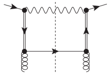
Figure 1: The $g^{*}q\to Zq$ process within the reggeized quark formalism. Double lines with arrow indicate the effective reggeized quark exchange in the $t$-channel.

within the reggeized quark formalism, the entire process is described using a single diagram, Fig. 1, with the $qq^{*}\to Z$ and $g^{*}q^{*}\to q$ sub-amplitudes connected by reggeized quark propagators,

$$=\frac{(\not{n}\not{p})_{\beta\alpha}}{2p\cdot n}\cdot\frac{i\cdot\not{q}}{{q}^{2}+i\epsilon} =\frac{(\not{p}\not{n})_{\alpha\beta}}{2p\cdot n}\cdot\frac{i\cdot\not{q}}{{q}^{2}+i\epsilon}\,.$$ (1)

While in the strict high-energy limit the $t$-channel four-momentum is purely transverse, $q^{2}=-{\bm{q}}^{2}$, generalizations to finite energies require to keep the full momentum dependence. The momenta $p$ and $n$ are light-cone momenta $p^{2}=n^{2}=0$ associated with the almost light-like momenta of scattering particles normalized to $2p\cdot n=s$, with $s$ the center-of-mass energy of the hadronic process. In e.g. deep-inelastic scattering, $n$ would be associated with the virtual photon and $p$ with the probed hadron. While (generalized) reggeized quark propagators carry at first explicit spin indices and therefore correlate the $qq^{*}\to Z$ and $g^{*}q^{*}\to q$ sub-amplitudes, it is possible to rewrite the high-energy projectors for the cross-section using

$$\frac{(\not{n}\not{p})_{\beta_{1}\alpha_{1}}(\not{p}\not{n})_{\alpha_{2}\beta_{2}}}{p\cdot n} =\not{p}_{\alpha_{1}\alpha_{2}}\not{n}_{\beta_{1}\beta_{2}}+(\gamma_{5}\not{p})_{\alpha_{1}\alpha_{2}}(\gamma_{5}\not{n})_{\beta_{1}\beta_{2}}.$$ (2)

For helicity independent input, the second term can be neglected and one remains with the projector $\not{p}_{\alpha_{1}\alpha_{2}}\not{n}_{\beta_{1}\beta_{2}}$ which then only contracts the Dirac indices of the $qq^{*}\to Z$ and $g^{*}q^{*}\to q$ sub-amplitudes respectively and therefore leads to a complete factorization of both processes.

3 Splitting functions from the 2 PI expansion in the axial gauge

The decomposition into 2PI diagrams as introduced in CFP80 is based on the use of axial i.e. light-cone gauge, which allows to analyze collinear singularities on the graph-by-graph basis EGMPR79 , in contrast to covariant gauges where such a rule is broken. Following CH94 , we will obtain TMD splitting functions which complete the set of already available evolution kernels. Unlike the case of the gluon-to-quark splitting treated in CH94 , the resulting splitting kernels have no direct definition as the coefficient of the BFKL Green’s function (or it is equivalent in the case of $t$-channel quark exchange). While the TMD quark-to-quark splitting can be identified as a certain next-to-leading order contributions to the high-energy resummed non-singlet $P_{qq}$ DGLAP splitting function, the TMD quark-to-gluon splitting is suppressed by a power of $x$ w.r.t. the leading logarithmic small-$x$ resummed $P_{gq}$ DGLAP splitting function. Nevertheless it is possible to attempt a definition of such quantities as matrix elements of reggeized quarks and conventional QCD degrees of freedom in light-cone gauge.

Following the framework set by CFP80 ; CH94 , the starting point for the definition of TMD splitting functions requires determination of the corresponding TMD splitting kernels,

$$\hat{K}_{ij}\left(z,\frac{\mathbf{k}^{2}}{\mu^{2}},\epsilon,\alpha_{s}\right) =\int\frac{dq^{2}d^{2+2\epsilon}{\bm{q}}}{2(2\pi)^{4+2\epsilon}}\Theta(\mu_{F}^{2}-q^{2})\mathbb{P}_{j,\,\text{in}}\otimes\hat{K}_{ij}^{(0)}(q,k)\otimes\mathbb{P}_{i,\,\text{out}}\,.$$ (3)

Here $\hat{K}_{ij}^{(0)}$, $i,j=q,g$ denotes the actual matrix element, describing the transition of parton $j$ to parton $i$, see Fig. 2, which is defined to include the propagators of outgoing lines. In case of gluons, these propagators are taken in $n\cdot A=0$ light-cone gauge; a similar statement applies to the polarization of real emitted gluons. $\mathbb{P}_{i,\,\text{in/out}}$ are on the other hand semi-projectors on incoming and outgoing lines. The symbol $\otimes$ represents contraction of indices and summation. $\mu_{F}$ denotes the factorization and dimensional regularization in $d=4+2\epsilon$ dimensions is employed with $\mu^{2}$ the dimensional regularization scale.

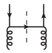
(a) $P_{qg}$

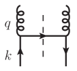
(b) $P_{gq}$

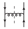
(c) $P_{qq}$

Figure 2: Matrix elements for the determination of splitting functions. Lower (incoming) lines carry always momentum $k$, upper (outgoing) lines carry momentum $q$.

The Sudakov parametrization for incoming and outgoing momenta, $k$ and $q$ (see fig. 2), reads

$$k^{\mu} =yp^{\mu}+k_{\perp}^{\mu}, q^{\mu} =xp^{\mu}+q_{\perp}^{\mu}+\frac{q^{2}+\mathbf{q}^{2}}{2x\,p\!\cdot\!n\,}n^{\mu}, \mathbf{\tilde{q}} =\mathbf{q}-z\mathbf{k},$$ (4)

with $z=x/y$. The semi-projectors on outgoing lines, $\mathbb{P}_{j,\,\text{out}}$, are directly taken from CFP80 :

$$\mathbb{P}_{g,\,\text{out}}^{\,\mu\nu} =-g^{\mu\nu} \mathbb{P}_{q,\,\text{out}} =\frac{\not{n}}{2\,q\!\cdot\!n\,}$$ (5)

While outgoing lines are at first treated in 1-1 correspondence to CFP80 , the on-shell restriction on incoming lines is now relaxed. The corresponding semi-projectors therefore require a slight modification. With the original projectors $\mathbb{P}_{j,\,\text{in}}$ of CFP80 ,

$$\mathbb{P}_{g,\,\text{in}}^{\text{\cite[cite]{\@@bibref{Authors Phrase1YearPhrase2}{CFP80}{\@@citephrase{(}}{\@@citephrase{)}}}}\,\mu\nu} =\frac{1}{m-2}\left(-g^{\mu\nu}+\frac{k^{\mu}n^{\nu}+n^{\mu}k^{\nu}}{\,k\!\cdot\!n\,}\right)\,, \mathbb{P}^{\text{\cite[cite]{\@@bibref{Authors Phrase1YearPhrase2}{CFP80}{\@@citephrase{(}}{\@@citephrase{)}}}}}_{q,\,\text{in}} =\frac{\not{k}}{2}\,,$$ (6)

are modified to

$$\mathbb{P}_{g,\,\text{in}}^{\,\mu\nu} =\frac{k_{\perp}^{\mu}k_{\perp}^{\nu}}{\mathbf{k}^{2}}\,, \mathbb{P}_{q,\,\text{in}} =\frac{y\,\not{p}}{2}\,.$$ (7)

While the modified gluon projector has been known since long time CH94 , we emphasize that the modified quark projector follows directly from the decomposition of the high energy projector in Eq. (2). Its normalization is on the other hand fixed by requiring agreement with the corresponding projector of CFP80 in the collinear limit. To ensure gauge invariance of the splitting functions in presence of off-shell momenta, it is further necessary to modify standard QCD vertices. The formalism which guarantees that gauge invariance holds is based on the reggeized quark formalism Lipatov:1995pn ; Lipatov:2000se ; Bogdan:2006af (for more recent re-derivation in spin helicity formalism see HKS13 ). The modification is achieved through adding certain eikonal terms which then in turn arrange gauge invariance of the vertex. Apart from the conventional QCD quark-quark-gluon vertex, $\Gamma^{\mu}_{qqg}=igt^{a}\gamma^{\mu}$ we have for the off-shell vertex with one reggeized quark $q^{*}$

$$\Gamma_{q^{*}qg}^{\mu}(p_{q^{*}},p_{q},p_{g}) =igt^{a}\left(\gamma^{\mu}+\frac{p^{\mu}}{\,p\!\cdot\!p_{g}\,}\not{p}_{q^{*}}\right) p_{q^{*}}\cdot p =0.$$ with (8)

Contracting the Lorentz index of this vertex with the gluon momentum yields $p_{g,\mu}\cdot\Gamma_{q^{*}qg}^{\mu}=-igt^{a}\not{p}_{q}$ which is equivalent to the corresponding expression for the conventional quark-quark-gluon vertex if the quark $p_{q}^{*}$ is taken on the mass shell. Moreover, in case the second quark is on the mass shell, we have immediately $p_{g,\mu}\cdot\Gamma_{q^{*}qg}^{\mu}\bar{u}(p_{q}^{\prime})=-igt^{a}\not{p}_{q}\bar{u}(p_{q}^{\prime})=0$ with $p_{q^{\prime}}^{2}=0$. We therefore find that using the generalized vertex Eq. (8), the current conservation holds despite of the quark with momentum $p_{q^{*}}$ being off-shell.

To determine both angular and transverse momentum dependent splitting functions,we start with Eq. (3), perform color, Dirac and Lorentz algebra, integrate over $q^{2}$ and shift the transverse momenta $\mathbf{q}\to\mathbf{\tilde{q}}=\mathbf{q}-z\mathbf{k}$, following closely the treatment in the seminal work of CH94 . We then obtain a set of angular- and transverse momentum dependent splitting functions $\tilde{P}_{ij}$ defined through

$$\hat{K}_{ij}\left(z,\frac{\mathbf{k}^{2}}{\mu_{F}^{2}},\epsilon,\alpha_{s}\right) =\frac{\alpha_{s}}{2\pi}\,z\,\int\frac{\mathrm{d}^{2+2\epsilon}\mathbf{\tilde{q}}^{2}}{\pi^{1+\epsilon}\mu^{2\epsilon}}\frac{e^{-\epsilon\gamma_{E}}}{\mathbf{\tilde{q}}^{2}}$$

$$\hskip 56.9055pt\Theta\left(\mu_{F}^{2}-\frac{\mathbf{\tilde{q}}^{2}+z(1-z)\mathbf{k}^{2}}{1-z}\right)\tilde{P}_{ij}^{(0)}\left(z,\mathbf{k},\mathbf{\tilde{q}},\epsilon\right)$$ (9)

with the $\overline{\text{MS}}$ scheme coupling $\alpha_{s}=\frac{g^{2}\mu^{2\epsilon}e^{\epsilon\gamma_{E}}}{(4\pi)^{1+\epsilon}}$ and $\gamma_{E}$ the Euler-Mascheroni constant. The angular and transverse momentum dependent splitting functions read

$$\tilde{P}_{gq}^{(0)}\left(z,\mathbf{k},\mathbf{\tilde{q}},\epsilon\right)=C_{\mathnormal{F}}\left(\frac{\mathbf{\tilde{q}}^{2}}{(\mathbf{\tilde{q}}^{2}+z(1-z)\mathbf{k}^{2})}\right)^{2}\left(\frac{\mathbf{\tilde{q}}^{2}}{(\mathbf{\tilde{q}}-(1-z)\mathbf{k})^{2}}\right)$$

$$\quad\times\Bigg{\{}\frac{2-2z+z^{2}}{z}+z(1-z)^{2}(1+z^{2})\left(\frac{\mathbf{k}^{2}}{\mathbf{\tilde{q}}^{2}}\right)^{2}+4(1-z)^{2}\left[\frac{\,\mathbf{k}\!\cdot\!\mathbf{\tilde{q}}\,}{\mathbf{\tilde{q}}^{2}}+z\left(\!\frac{\,\mathbf{k}\!\cdot\!\mathbf{\tilde{q}}\,}{\mathbf{\tilde{q}}^{2}}\!\right)^{2}\right]$$

$$\quad+4z^{2}(1-z)^{2}\frac{\,\mathbf{k}\!\cdot\!\mathbf{\tilde{q}}\,\mathbf{k}^{2}}{\mathbf{\tilde{q}}^{4}}+2(1-z)(1+z-z^{2})\frac{\mathbf{k}^{2}}{\mathbf{\tilde{q}}^{2}}\Bigg{\}}+C_{\mathnormal{F}}\frac{\epsilon\,z\mathbf{\tilde{q}}^{2}(\mathbf{\tilde{q}}-(1-z)\mathbf{k})^{2}}{(\mathbf{\tilde{q}}^{2}+z(1-z)\mathbf{k}^{2})^{2}},$$ (10)

$$\tilde{P}_{qg}^{(0)}\left(z,\mathbf{k},\mathbf{\tilde{q}},\epsilon\right)=T_{\mathnormal{R}}\left(\frac{\mathbf{\tilde{q}}^{2}}{\mathbf{\tilde{q}}^{2}+z(1-z)\mathbf{k}^{2}}\right)^{2}$$

$$\qquad\quad\times\Bigg{[}1+4z^{2}(1-z)^{2}\frac{\mathbf{k}^{2}}{\mathbf{\tilde{q}}^{2}}+4z(1-z)(1-2z)\frac{\,\mathbf{k}\!\cdot\!\mathbf{\tilde{q}}\,}{\mathbf{\tilde{q}}^{2}}-4z(1-z)\left(\!\frac{\,\mathbf{k}\!\cdot\!\mathbf{\tilde{q}}\,}{\sqrt{\mathbf{\tilde{q}}^{2}\mathbf{k}^{2}}}\!\right)^{2}\Bigg{]},$$ (11)

$$\tilde{P}_{qq}^{(0)}\left(z,\mathbf{k},\mathbf{\tilde{q}},\epsilon\right)=C_{\mathnormal{F}}\left(\frac{\mathbf{\tilde{q}}^{2}}{(\mathbf{\tilde{q}}^{2}+z(1-z)\mathbf{k}^{2})}\right)^{2}\left(\frac{\mathbf{\tilde{q}}^{2}}{(\mathbf{\tilde{q}}-(1-z)\mathbf{k})^{2}}\right)$$

$$\quad\times\Bigg{\{}\frac{1+z^{2}}{1-z}+z^{2}(1-z)(5-4z+z^{2})\left(\frac{\mathbf{k}^{2}}{\mathbf{\tilde{q}}^{2}}\right)^{2}-4z(1-z)^{2}\left(\!\frac{\,\mathbf{k}\!\cdot\!\mathbf{\tilde{q}}\,}{\mathbf{\tilde{q}}^{2}}\!\right)^{2}$$

$$\quad+2z(1-2z)\frac{\,\mathbf{k}\!\cdot\!\mathbf{\tilde{q}}\,}{\mathbf{\tilde{q}}^{2}}+2z(2-7z+7z^{2}-2z^{3})\frac{\mathbf{k}^{2}\,\mathbf{k}\!\cdot\!\mathbf{\tilde{q}}\,}{\mathbf{\tilde{q}}^{4}}+(1+z+4z^{2}-2z^{3})\frac{\mathbf{k}^{2}}{\mathbf{\tilde{q}}^{2}}$$

$$\qquad+\epsilon(1-z)\cdot\bigg{[}1-2(1-2z)\frac{\mathbf{k}\cdot\mathbf{\tilde{q}}}{\mathbf{\tilde{q}}^{2}}-4z(1-z)\left(\frac{\mathbf{k}\cdot\mathbf{\tilde{q}}}{\mathbf{\tilde{q}}^{2}}\right)^{2}+(1-2z+2z^{2})\frac{\mathbf{k}^{2}}{\mathbf{\tilde{q}}^{2}}$$

$$\qquad\hskip 113.81102pt+z(1-z)(1-2z)\frac{\mathbf{k}\cdot\mathbf{\tilde{q}}\mathbf{k}^{2}}{\mathbf{\tilde{q}}^{4}}+z^{2}(1-z)^{2}\left(\frac{\mathbf{k}^{2}}{\mathbf{\tilde{q}}^{2}}\right)^{2}\bigg{]}\Bigg{\}}.$$ (12)

Determination of both angular and transverse momentum dependent splitting functions for the splittings quark-to-gluon and quark-to-quark present, together with the results presented further down in Sec. 5, the central results of this work.

4 Gauge invariance of TMD splitting functions

The obtained TMD splitting functions will be essential for the definition of set of TMD evolution equations of TMD parton distributions. While the above derivation is based on the 2PI-expansion of CFP80 the derivation might be at first regarded as not completely satisfactory. While care has been taken to ensure gauge invariance of the off-shell vertex Eq. (8), the employed formalism heavily relies on the use of the light-cone gauge and gauge invariance of our result is not immediately apparent. This is of particular concern, once we relax the integration over $\tilde{\bm{q}}$ in Eq. (23) to allow for TMD factorization in the outgoing momentum $\tilde{\bm{q}}$ and therefore leave strictly speaking the framework provided by CFP80 . To ensure gauge invariance also in this more general case, we will provide in the following an explicit gauge invariant extension of the sub-amplitudes Fig. 2 as well as the projectors. As a consequence we will both obtain explicitly gauge invariant sub-amplitudes and verify that any possible gauge dependence hidden in the propagators of the outgoing parton with momentum $q$ and/or the real produced parton with momentum $p^{\prime}=k-q$ will cancel. In particular, while calculations are no longer restricted to the light-cone gauge as in Sec. 3, they agree at every stage precisely with the results derived in this gauge. To this end we first generalize the projector of the outgoing gluon in Eq. (5). Another source of potential violation of gauge invariance is due to the use of explicit cut-offs in Eq. (3). A generalization of our results to a cut-off-independent formulation is left at this stage as a task for future research, restricting ourselves for the time being to the proper definition of gauge-invariant sub-amplitudes.

With the polarization tensor of the gluon propagator in the light-cone gauge given by

$$\Delta_{\mu\mu^{\prime}}(q)=-g_{\mu\mu^{\prime}}+\frac{q^{\mu^{\prime}}n^{\mu}+n^{\mu^{\prime}}q^{\mu}}{q\cdot n},$$ (13)

we define the new projector

$$\tilde{\mathbb{P}}_{g,\,\text{out}}^{\,\mu\nu}(q,n) \equiv\Delta_{\mu\mu^{\prime}}(q)\mathbb{P}_{g,\,\text{out}}^{\,\mu^{\prime}\nu^{\prime}}\Delta_{\nu^{\prime}\nu}(q)=-g_{\mu\nu}+\frac{q^{\mu}n^{\nu}+n^{\mu}q^{\nu}}{q\cdot n}-q^{2}\frac{n^{\mu}n^{\nu}}{(q\cdot n)^{2}},$$ (14)

which fulfills the following properties:

$$0 =\tilde{\mathbb{P}}_{g,\,\text{out}}^{\,\mu\nu}\cdot q_{\mu}=\tilde{\mathbb{P}}_{g,\,\text{out}}^{\,\mu\nu}\cdot q_{\nu}=\tilde{\mathbb{P}}_{g,\,\text{out}}^{\,\mu\nu}\cdot n_{\mu}=\tilde{\mathbb{P}}_{g,\,\text{out}}^{\,\mu\nu}\cdot n_{\nu}\,.$$ (15)

Furthermore

$$\tilde{\mathbb{P}}_{g,\,\text{out}}^{\,\mu\nu}\cdot q_{\perp}^{\mu}q_{\perp}^{\nu}={\bm{q}}^{2}$$ (16)

and hence the combination

$$\tilde{\mathbb{P}}_{g,\,\text{out}}^{\,\mu\nu}(q,n)\tilde{\mathbb{P}}_{g,\,\text{in}}^{\,\mu^{\prime}\nu^{\prime}}(q_{\perp}),$$ (17)

is indeed a projector. Due to the properties Eq. (15), one also has

$$\tilde{\mathbb{P}}_{g,\,\text{out}}^{\,\mu\nu^{\prime}}(q,n)\Delta_{\nu^{\prime}\nu}(q)=\tilde{\mathbb{P}}_{g,\,\text{out}}^{\,\mu\nu^{\prime}}(q,n)=\Delta_{\mu\mu^{\prime}}(q)\tilde{\mathbb{P}}_{g,\,\text{out}}^{\,\mu^{\prime}\nu}(q,n)\,.$$ (18)

Using therefore Eq. (14) in the analysis of the previous section, will leave our results unchanged. The second modification concerns the sub-amplitudes Fig. 2. In the high energy limit, corresponding gauge invariant vertices can be easily derived within the reggeized quark formalism. To ensure gauge invariance in presence of both off-shell momenta $k$ and $q$, with $q$ of the general form Eq. (4), these vertices require a slight generalization, similar to the one employed already in Hautmann:2012sh . The version to be used in the following reads

$$\Gamma_{q^{*}g^{*}q}^{\mu}(q,k,p^{\prime}) =igt^{a}\left(\gamma^{\mu}-\frac{n^{\mu}}{\,k\!\cdot\!n\,}\not{q}\right),$$ (19)

$$\Gamma_{g^{*}q^{*}q}^{\mu}(q,k,p^{\prime}) =igt^{a}\left(\gamma^{\mu}-\frac{p^{\mu}}{\,p\!\cdot\!q\,}\not{k}\right),$$ (20)

$$\Gamma_{q^{*}q^{*}g}^{\mu}(q,k,p^{\prime}) =igt^{a}\left(\gamma^{\mu}-\frac{p^{\mu}}{\,p\!\cdot\!p^{\prime}\,}\not{k}+\frac{n^{\mu}}{\,n\!\cdot\!p^{\prime}\,}\not{q}\right).$$ (21)

where we used $p^{\prime}=k-q$ for the momentum of the real produced particle and $q^{*}$, $g^{*}$indicate an off-shell quark and gluon; the momentum $k$ and momentum $q$ refer always to incoming and outgoing particles respectively. In particular, these vertices obey

$${k}_{\mu}\cdot\Gamma^{\mu}_{q^{*}g^{*}q}(k,q)\bar{u}(p^{\prime}) =0 {q}_{\mu}\cdot\Gamma^{\mu}_{q^{*}q^{*}g}(k,q)\bar{u}(p^{\prime}) =0 {p^{\prime}}_{\mu}\cdot\Gamma^{\mu}_{q^{*}q^{*}g}(k,q) =0\,.$$ (22)

Due to these properties, any gauge dependence induced by either the polarization tensor of a $t$-channel gluon with momentum $q$, a real produced gluon with momentum $p^{\prime}=k-q$, or a $t$-channel gluon with momentum $k$ is canceled and the overall result is gauge-invariant. In particular it is trivial to check that the results obtained in the previous section using the light-cone gauge, generalize directly to the present formulation. A last comment is in order concerning the universality of our results. As pointed out in the beginning of Sec. 3, unlike the splitting function of CH94 , our splitting functions cannot be uniquely associated with the e.g. next-to-leading order coefficient of the small-$x$ gluon Green’s function etc. Indeed there will be always contributions of similar order of magnitude than elements of our splitting functions, which are not contained in its definition. Our splitting functions comprise however a set of contributions which

• reduces in the collinear limit to collinear splitting functions

• reduces in the high energy limit to corresponding high energy factorized expressions (guaranteed through the use of the reggeized quark and gluon vertices)

• combines both limits in a gauge invariant way.

It is then the combination of these three requirements which provides strong constraints on the terms contained in the definition of our TMD splitting functions.

5 Angular averaged TMD splitting functions and singularity structure

In the following section we further analyze our results of Sec. 3. While the explicit angular-momentum-dependence of our results might be of interest for further Monte-Carlo realizations which aim at description of exclusive final states, the evolution of TMD parton distribution functions generally requires only angular-averaged splitting functions. Furthermore, the splitting functions turn out to be divergent in certain regions of phase space, which will be identified below.

5.1 Angular averaged TMD splitting functions

To arrive at a result similar to the one obtained in CH94 for the TMD $P_{qg}$, it is further necessary to average over the azimuthal angle. With

$$\hat{K}_{ij}\left(z,\frac{\mathbf{k}^{2}}{\mu_{F}^{2}},\alpha_{s},\epsilon\right) =\frac{\alpha_{s}}{2\pi}\,z\!\!\!\int\limits_{0}^{(1-z)(\mu_{F}^{2}-z\mathbf{k}^{2})}\frac{\mathrm{d}\mathbf{\tilde{q}}^{2}}{\mathbf{\tilde{q}}^{2}}\left(\frac{\mathbf{\tilde{q}}^{2}}{\mu^{2}}\right)^{\epsilon}\frac{e^{-\epsilon\gamma_{E}}}{\Gamma(1+\epsilon)}{P}_{ij}^{(0)}\left(z,\frac{\mathbf{k}^{2}}{\mathbf{\tilde{q}}^{2}},\epsilon\right),$$ (23)

which then defines the TMD splitting functions $P_{ij}$, we reproduce for the gluon-to-quark splitting the result of CH94 , also calculated in Ciafaloni:2005cg ; Hautmann:2012sh

$$P_{qg}^{(0)}\left(z,\frac{\mathbf{k}^{2}}{\mathbf{\tilde{q}}^{2}},\epsilon\right) =T_{\mathnormal{R}}\left(\frac{\mathbf{\tilde{q}}^{2}}{\mathbf{\tilde{q}}^{2}+z(1-z)\,\mathbf{k}^{2}}\right)^{2}\Bigg{[}z^{2}+(1-z)^{2}+4z^{2}(1-z)^{2}\frac{\mathbf{k}^{2}}{\mathbf{\tilde{q}}^{2}}\Bigg{]}.$$ (24)

For the new TMD splitting functions we obtain

$${P}_{gq}^{(0)}\left(z,\frac{\mathbf{k}^{2}}{\mathbf{\tilde{q}}^{2}},\epsilon\right) =C_{F}\Bigg{[}\frac{2\mathbf{\tilde{q}}^{2}}{z|\mathbf{\tilde{q}}^{2}-(1-z)^{2}\mathbf{k}^{2}|}$$

$$\hskip 56.9055pt-\frac{\mathbf{\tilde{q}}^{2}(\mathbf{\tilde{q}}^{2}(2-z)+\mathbf{k}^{2}z(1-z^{2}))-\epsilon z(\mathbf{\tilde{q}}^{2}+(1-z)^{2}\mathbf{k}^{2})}{(\mathbf{\tilde{q}}^{2}+z(1-z)\mathbf{k}^{2})^{2}}\Bigg{]},$$ (25)

$${P}_{qq}^{(0)}\left(z,\frac{\mathbf{k}^{2}}{\mathbf{\tilde{q}}^{2}},\epsilon\right) =C_{\mathnormal{F}}\left(\frac{\mathbf{\tilde{q}}^{2}}{\mathbf{\tilde{q}}^{2}+z(1-z)\mathbf{k}^{2}}\right)\bigg{[}\frac{\mathbf{\tilde{q}}^{2}+(1-z^{2})\mathbf{k}^{2}}{(1-z)|\mathbf{\tilde{q}}^{2}-(1-z)^{2}\mathbf{k}^{2}|}$$

$$\hskip 36.98866pt+\frac{z^{2}\mathbf{\tilde{q}}^{2}-z(1-z)(1-3z+z^{2})\mathbf{k}^{2}+(1-z)^{2}\epsilon(\mathbf{\tilde{q}}^{2}+z^{2}\mathbf{k}^{2})}{(1-z)(\mathbf{\tilde{q}}^{2}+z(1-z)\mathbf{k}^{2})}\bigg{]}\,.$$ (26)

As expected from our method to construct TMD splitting functions, we obtain in the collinear limit ($\mathbf{k}^{2}/\mathbf{\tilde{q}}^{2}\to 0$) the well-known real parts of the leading-order Altarelli-Parisi splitting functions in $d=4+2\epsilon$ dimensions:

$$P_{gq}^{(0)}(z,0,\epsilon) =C_{\mathnormal{F}}\frac{1+(1-z)^{2}+\epsilon z^{2}}{z},$$ (27)

$$P_{qg}^{(0)}(z,0,\epsilon) =T_{\mathnormal{R}}\left(z^{2}+(1-z)^{2}\right),$$ (28)

$$P_{qq}^{(0)}(z,0,\epsilon) =C_{\mathnormal{F}}\,\frac{1+z^{2}+\epsilon(1-z)^{2}}{1-z}.$$ (29)

5.2 Singularity structure of the TMD splitting functions

Unlike the $P_{qg}$ TMD splitting function, the splitting functions in Eq. (24) and Eq. (5.1) develop singularities in certain regions of phase space. These singularities can be organized into two groups: those associated with the limit $z\to 1$, only present for the splitting $P_{qq}$, and those associated with the limit $|\mathbf{\tilde{q}}|\to(1-z)|\mathbf{k}|$, present for both $P_{gq}$ and $P_{qq}$. The coefficient of the $z\to 1$ singularity reads

$$\lim_{z\to 1}P_{qq}^{(0)}\left(z,\frac{\mathbf{k}^{2}}{\mathbf{\tilde{q}}^{2}}\right) =C_{\mathnormal{F}}\frac{2}{1-z}$$ (30)

and coincides with the $z\to 1$ singularity of the conventional collinear splitting functions where it is known to be regularized by corresponding virtual corrections to the splitting kernel. We expect a similar mechanism to be realized in the case of the $P_{qq}$ splitting kernel with full transverse momentum dependence. The nature of the second singularity is more intriguing, since it is present for both diagonal ($P_{qq}$ ) and off-diagonal ($P_{gq}$) splitting kernels. The coefficients of this singularity is provided by

$$\lim_{|\mathbf{\tilde{q}}|\to(1-z)|\mathbf{k}|}P_{gq}^{(0)}\left(z,\frac{\mathbf{k}^{2}}{\mathbf{\tilde{q}}^{2}},\epsilon\right) =\frac{2C_{\mathnormal{F}}}{z}\frac{\mathbf{\tilde{q}}^{2}}{|\mathbf{\tilde{q}}^{2}-(1-z)^{2}\mathbf{k}^{2}|}$$

$$\lim_{|\mathbf{\tilde{q}}|\to(1-z)|\mathbf{k}|}P_{qq}^{(0)}\left(z,\frac{\mathbf{k}^{2}}{\mathbf{\tilde{q}}^{2}},\epsilon\right) =\frac{2C_{\mathnormal{F}}}{1-z}\frac{\mathbf{\tilde{q}}^{2}}{|\mathbf{\tilde{q}}^{2}-(1-z)^{2}\mathbf{k}^{2}|}$$ (31)

For the $P_{qq}$ splitting function, this singularity always overlaps with the $z\to 1$ singularity. At the level of the angular-dependent splitting kernels Eq. (3) and Eq. (3), this singularity is easily identified with the vanishing of the transverse momentum of the real, emitted parton i.e. of the real gluon ($P_{qq}$) and of the real quark ($P_{gq}$) respectively. To analyze the precise structure of the singularities within dimensional regularization it is convenient to switch to the re-scaled momentum $\mathbf{\tilde{p}}=\frac{\mathbf{k}-\mathbf{q}}{1-z}$ instead of $\mathbf{\tilde{q}}$. We then obtain

$$\hat{K}_{qq}\left(z,\frac{\mathbf{k}^{2}}{\mu_{F}^{2}},\alpha_{s}\right) =\frac{\alpha_{s}}{2\pi}z\int\frac{d^{2+2\epsilon}\mathbf{\tilde{p}}}{\pi^{1+\epsilon}\mu^{2\epsilon}}\,e^{-\epsilon\gamma_{E}}\,\Theta\left(\mu_{F}^{2}-(1-z)(\mathbf{\tilde{p}}-\mathbf{k})^{2}-z\mathbf{k}^{2}\right)$$

$$\hskip 45.52458pt\Bigg{\{}\frac{1}{(1-z)^{1-2\epsilon}}\left(\frac{1}{\mathbf{\tilde{p}}^{2}}+\frac{\mathbf{k}^{2}+z(1-z)\mathbf{\tilde{p}}^{2}}{\mathbf{\tilde{p}}^{2}[(1-z)(\mathbf{\tilde{p}}-\mathbf{k})^{2}+z\mathbf{k}^{2}]}\right)$$

$$\hskip 45.52458pt-\frac{\mathbf{\tilde{p}}^{2}z(1-z)^{2+2\epsilon}(1+\epsilon)}{[(1-z)(\mathbf{\tilde{p}}-\mathbf{k})^{2}+z\mathbf{k}^{2}]^{2}}+\frac{\epsilon(1-z)^{1+2\epsilon}}{(1-z)(\mathbf{\tilde{p}}-\mathbf{k})^{2}+z\mathbf{k}^{2}}\Bigg{\}}$$ (32)

$$\hat{K}_{gq}\left(z,\frac{\mathbf{k}^{2}}{\mu_{F}^{2}},\alpha_{s}\right) =\frac{\alpha_{s}}{2\pi}z\int\frac{d^{2+2\epsilon}\mathbf{\tilde{p}}}{\pi^{1+\epsilon}\mu^{2\epsilon}}\,e^{-\epsilon\gamma_{E}}\,\Theta\left(\mu_{F}^{2}-(1-z)(\mathbf{\tilde{p}}-\mathbf{k})^{2}-z\mathbf{k}^{2}\right)$$

$$\hskip 45.52458pt\Bigg{\{}\frac{(1-z)^{2\epsilon}}{z}\frac{2}{\mathbf{\tilde{p}}^{2}}+\frac{\mathbf{\tilde{p}}^{2}z(1-z)^{2+2\epsilon}(1+\epsilon)}{[(1-z)(\mathbf{\tilde{p}}-\mathbf{k})^{2}+z\mathbf{k}^{2}]^{2}}$$

$$\hskip 176.407pt-\frac{2(1-z)^{1+2\epsilon}}{(1-z)(\mathbf{\tilde{p}}-\mathbf{k})^{2}+z\mathbf{k}^{2}}\Bigg{\}}$$ (33)

It is now possible to isolate the singularities of interest using a phase space slicing parameter $\lambda\to 0$ which splits the integration over $\mathbf{\tilde{p}}$ into regions $|\mathbf{\tilde{p}}|<\lambda$, $|\mathbf{\tilde{p}}|>\lambda$. Defining $K_{qq}^{(0)\text{fin.}}$ and $K_{gq}^{(0)\text{fin.}}$ as the kernels given in Eq. (5.2) and Eq. (5.2), but with the integration measure $d^{2+2\epsilon}\mathbf{\tilde{p}}$ replaced appropriately by $d^{2+2\epsilon}\mathbf{\tilde{p}}\cdot\Theta(\mathbf{\tilde{p}}^{2}-\lambda^{2})$ and $d^{2+2\epsilon}\mathbf{\tilde{p}}\cdot\Theta(\lambda^{2}-\mathbf{\tilde{p}}^{2})$ we have

$$\hat{K}_{qq}\left(z,\frac{\mathbf{k}^{2}}{\mu_{F}^{2}},\alpha_{s},\epsilon\right) =\hat{K}_{qq}^{\text{fin.}}\left(z,\frac{\mathbf{k}^{2}}{\mu_{F}^{2}},\alpha_{s},\epsilon\right)+\hat{K}_{qq}^{\text{div.}}\left(z,\frac{\mathbf{k}^{2}}{\mu_{F}^{2}},\alpha_{s},\epsilon\right)$$

$$\hat{K}_{gq}\left(z,\frac{\mathbf{k}^{2}}{\mu_{F}^{2}},\alpha_{s},\epsilon\right) =\hat{K}_{gq}^{\text{fin.}}\left(z,\frac{\mathbf{k}^{2}}{\mu_{F}^{2}},\alpha_{s},\epsilon\right)+\hat{K}_{gq}^{\text{div.}}\left(z,\frac{\mathbf{k}^{2}}{\mu_{F}^{2}},\alpha_{s},\epsilon\right)$$ (34)

with

$$\hat{K}_{qq}^{\text{div.}}\left(z,\frac{\mathbf{k}^{2}}{\mu_{F}^{2}},\alpha_{s},\epsilon\right) =\frac{\alpha_{s}}{\pi}\Theta(\mu_{F}^{2}-\mathbf{k}^{2})\frac{e^{-\epsilon\gamma_{E}}}{\Gamma(1+\epsilon)}\frac{\lambda^{2\epsilon}}{\epsilon(1-z)^{1-2\epsilon}}+\mathcal{O}(\lambda)$$

$$=\frac{\alpha_{s}}{\pi}\Theta(\mu_{F}^{2}-\mathbf{k}^{2})\frac{e^{-\epsilon\gamma_{E}}}{\Gamma(1+\epsilon)}\left(\frac{\lambda^{2}}{\mu^{2}}\right)^{\epsilon}\frac{1}{\epsilon}\left(\frac{1}{2\epsilon}\delta(1-z)+\frac{1}{(1-z)_{+}^{1-2\epsilon}}\right)+\mathcal{O}(\lambda)$$

$$\hat{K}_{gq}^{\text{div.}}\left(z,\frac{\mathbf{k}^{2}}{\mu_{F}^{2}},\alpha_{s}\right) =\frac{\alpha_{s}}{\pi}\Theta(\mu_{F}^{2}-\mathbf{k}^{2})\frac{e^{-\epsilon\gamma_{E}}}{\Gamma(1+\epsilon)}\left(\frac{\lambda^{2}}{\mu^{2}}\right)^{\epsilon}\frac{\left((1-z)\right)^{2\epsilon}}{\epsilon z}+\mathcal{O}(\lambda)$$ (35)

where we made use of the limit $\lambda\to 0$. We furthermore introduced the usual plus-prescription

$$\int_{0}^{1}dz\frac{f(z)}{(1-z)_{+}} \equiv\int_{0}^{1}dz\frac{f(z)-f(1)}{(1-z)},$$ (36)

and made use of the identity

$$\frac{1}{(1-z)^{1-2\epsilon}} =\frac{1}{2\epsilon}\delta(1-z)+\frac{1}{(1-z)_{+}^{1-2\epsilon}}$$

$$=\frac{1}{2\epsilon}\delta(1-z)+\frac{1}{(1-z)_{+}}+2\epsilon\left(\frac{\ln(1-z)}{(1-z)}\right)_{+}+\mathcal{O}(\epsilon^{2})\,.$$ (37)

Note that since the real emitted particle is on-shell, the vanishing of its transverse momentum $\mathbf{\tilde{p}}$ implies also vanishing of the component parallel to $n$. As a consequence the momentum of the emitted particle is in this case collinear to the initial proton momentum $p$. For a hands-on approach, it appears therefore to be natural to avoid this singularity by introducing a cut-off, similar to $\lambda$ in the $K_{qq}^{(0)\text{fin.}}$ and $K_{gq}^{(0)\text{fin.}}$ terms or by imposing an angular ordering inspired constrained on the $t$-channel momenta such as $|\mathbf{\tilde{q}}|/(1-z)>|\mathbf{k}|$ which avoids the singular region. Such a treatment would then allow for first numerical tests of the proposed TMD splitting functions and for their application to phenomenological studies. A complete theoretical treatment of this singularity would on the other hand require the determination of virtual corrections (in the case of the $P_{qq}$ splitting) and most likely the realization of a systematic subtraction mechanism which removes parton emission collinear to the initial proton momentum from the TMD splitting kernels. Both tasks are beyond the scope of this work and are left as a task for future research.

6 Summary and Outlook

In this paper we extended the method developed by Catani and Hautmann for the determination of transverse-momentum-dependent parton splitting functions to splittings of initial $k_{T}$-dependent quarks, based on factorization of cross-sections in the high energy limit. Gauge invariance of underlying amplitudes in presence of off-shell partons is achieved due to the reggeized quark calculus, which supplements conventional QCD vertices by certain eikonal contributions. While our approach is heavily based on the 2PI expansion in the light-cone gauge by Curci et al., we have been able to verify that it is possible to generalize the employed projectors in a way, such that the choice of gauge for the sub-amplitudes, which underlie the derivation of our splitting kernels, becomes irrelevant i.e. our TMD splitting kernels are independent of the employed gauge. While our splitting kernels are in this way well defined objects, there are not necessarily universal, since they cannot be directly defined as the coefficients of e.g. the high energy resummation of a certain TMD parton distribution function, such as the TMD gluon-to-quark splitting functions. They are merely constrained by the requirement to reduce in the collinear and high energy limit to the well-known exact expressions.

The current study determines only the real contribution to the TMD quark-to-quark and quark-to-gluon splitting kernels. Future studies will have to focus on the determination of the corresponding virtual corrections for the TMD quark-to-quark splitting function, the development of a coherent framework which allows for a systematic subtraction of singularities not canceled by virtual corrections and finally the formulation of appropriate coupled evolution equations for TMD parton distribution functions. As a long term goal, a matching of TMD evolution based on factorization in the soft-collinear limit, see e.g. Collins:2014jpa ; Echevarria:2012pw ; Becher:2010tm is a task which needs to be addressed.

References

- (1) R. Angeles-Martinez et al., Transverse momentum dependent (TMD) parton distribution functions: status and prospects, arXiv:1507.0526.
- (2) J. Collins, Foundations of perturbative QCD. Cambridge University Press, 2011.
- (3) I. Balitsky and A. Tarasov, Rapidity evolution of gluon TMD from low to moderate x, JHEP 10 (2015) 017, [arXiv:1505.0215].
- (4) F. Dominguez, C. Marquet, B.-W. Xiao, and F. Yuan, Universality of Unintegrated Gluon Distributions at small x, Phys. Rev. D83 (2011) 105005, [arXiv:1101.0715].
- (5) P. Kotko, K. Kutak, C. Marquet, E. Petreska, S. Sapeta, and A. van Hameren, Improved TMD factorization for forward dijet production in dilute-dense hadronic collisions, JHEP 09 (2015) 106, [arXiv:1503.0342].
- (6) Y. V. Kovchegov and M. D. Sievert, Calculating TMDs of an Unpolarized Target: Quasi-Classical Approximation and Quantum Evolution, arXiv:1505.0117.
- (7) S. Catani, M. Ciafaloni, and F. Hautmann, High-energy factorization and small x heavy flavor production, Nucl. Phys. B366 (1991) 135–188.
- (8) M. Deak, F. Hautmann, H. Jung, and K. Kutak, Forward Jets and Energy Flow in Hadronic Collisions, Eur. Phys. J. C72 (2012) 1982, [arXiv:1112.6354].
- (9) M. Deak, F. Hautmann, H. Jung, and K. Kutak, Forward-Central Jet Correlations at the Large Hadron Collider, arXiv:1012.6037.
- (10) G. Chachamis, M. Deak, M. Hentschinski, G. Rodrigo, and A. Sabio Vera, Single bottom quark production in k⊥-factorisation, JHEP 09 (2015) 123, [arXiv:1507.0577].
- (11) S. Dooling, F. Hautmann, and H. Jung, Hadroproduction of electroweak gauge boson plus jets and TMD parton density functions, Phys. Lett. B736 (2014) 293–298, [arXiv:1406.2994].
- (12) F. Hautmann, M. Hentschinski, and H. Jung, Forward Z-boson production and the unintegrated sea quark density, Nucl.Phys. B865 (2012) 54–66, [arXiv:1205.1759].
- (13) A. van Hameren, P. Kotko, and K. Kutak, Resummation effects in the forward production of Z0+jet at the LHC, Phys. Rev. D92 (2015), no. 5 054007, [arXiv:1505.0276].
- (14) M. Ciafaloni, Coherence Effects in Initial Jets at Small q**2 / s, Nucl.Phys. B296 (1988) 49.
- (15) G. Marchesini, QCD coherence in the structure function and associated distributions at small x, Nucl. Phys. B445 (1995) 49–80, [hep-ph/9412327].
- (16) S. Catani, F. Fiorani, and G. Marchesini, Small x Behavior of Initial State Radiation in Perturbative QCD, Nucl.Phys. B336 (1990) 18.
- (17) S. Catani, F. Fiorani, and G. Marchesini, QCD Coherence in Initial State Radiation, Phys.Lett. B234 (1990) 339.
- (18) H. Jung, S. Baranov, M. Deak, A. Grebenyuk, F. Hautmann, et al., The CCFM Monte Carlo generator CASCADE version 2.2.03, Eur.Phys.J. C70 (2010) 1237–1249, [arXiv:1008.0152].
- (19) F. Hautmann and H. Jung, Transverse momentum dependent gluon density from DIS precision data, Nucl. Phys. B883 (2014) 1–19, [arXiv:1312.7875].
- (20) K. Kutak and S. Sapeta, Gluon saturation in dijet production in p-Pb collisions at Large Hadron Collider, Phys.Rev. D86 (2012) 094043, [arXiv:1205.5035].
- (21) K. Kutak, Hard scale dependent gluon density, saturation and forward-forward dijet production at the LHC, Phys. Rev. D91 (2015), no. 3 034021, [arXiv:1409.3822].
- (22) J. Kwiecinski, A. D. Martin, and A. M. Stasto, A Unified BFKL and GLAP description of F2 data, Phys. Rev. D56 (1997) 3991–4006, [hep-ph/9703445].
- (23) A. van Hameren, P. Kotko, K. Kutak, and S. Sapeta, Small- dynamics in forward-central dijet decorrelations at the LHC, Phys. Lett. B737 (2014) 335–340, [arXiv:1404.6204].
- (24) H. Jung, F. Hautmann, and A. Lelek, TMD MC CASCADE, REF conference 2015, .
- (25) S. Catani and F. Hautmann, High-energy factorization and small x deep inelastic scattering beyond leading order, Nucl.Phys. B427 (1994) 475–524, [hep-ph/9405388].
- (26) G. Curci, W. Furmanski, and R. Petronzio, Evolution of parton densities beyond leading order: the nonsinglet case, Nucl.Phys. B175 (1980) 27.
- (27) S. Jadach, A. Kusina, M. Skrzypek, and M. Slawinska, Two real parton contributions to non-singlet kernels for exclusive QCD DGLAP evolution, JHEP 08 (2011) 012, [arXiv:1102.5083].
- (28) S. Jadach, A. Kusina, W. Placzek, M. Skrzypek, and M. Slawinska, Inclusion of the QCD next-to-leading order corrections in the quark-gluon Monte Carlo shower, Phys. Rev. D87 (2013), no. 3 034029, [arXiv:1103.5015].
- (29) O. Gituliar, Higher-Order Corrections in QCD Evolution Equations and Tools for Their Calculation. PhD thesis, Cracow, INP, 2014. arXiv:1403.6897.
- (30) O. Gituliar, S. Jadach, A. Kusina, and M. Skrzypek, On regularizing the infrared singularities in QCD NLO splitting functions with the new Principal Value prescription, Phys. Lett. B732 (2014) 218–222, [arXiv:1401.5087].
- (31) L. N. Lipatov and M. I. Vyazovsky, QuasimultiRegge processes with a quark exchange in the t channel, Nucl. Phys. B597 (2001) 399–409, [hep-ph/0009340].
- (32) L. Lipatov, Gauge invariant effective action for high-energy processes in QCD, Nucl.Phys. B452 (1995) 369–400, [hep-ph/9502308].
- (33) M. Hentschinski and A. Sabio Vera, NLO jet vertex from Lipatov’s QCD effective action, Phys. Rev. D85 (2012) 056006, [arXiv:1110.6741].
- (34) M. Hentschinski, Pole prescription of higher order induced vertices in Lipatov’s QCD effective action, Nucl. Phys. B859 (2012) 129–142, [arXiv:1112.4509].
- (35) G. Chachamis, M. Hentschinski, J. D. Madrigal Martinez, and A. Sabio Vera, Quark contribution to the gluon Regge trajectory at NLO from the high energy effective action, Nucl. Phys. B861 (2012) 133–144, [arXiv:1202.0649].
- (36) G. Chachamis, M. Hentschinski, J. D. Madrigal Martínez, and A. S. Vera, Next-to-leading order corrections to the gluon-induced forward jet vertex from the high energy effective action, Phys. Rev. D87 (2013), no. 7 076009, [arXiv:1212.4992].
- (37) G. Chachamis, M. Hentschinski, J. D. Madrigal Martinez, and A. Sabio Vera, Gluon Regge trajectory at two loops from Lipatov’s high energy effective action, Nucl. Phys. B876 (2013) 453–472, [arXiv:1307.2591].
- (38) M. Hentschinski, J. D. Madrigal Martinez, B. Murdaca, and A. Sabio Vera, The next-to-leading order vertex for a forward jet plus a rapidity gap at high energies, Phys. Lett. B735 (2014) 168–172, [arXiv:1404.2937].
- (39) M. Hentschinski, J. D. Madrigal Martinez, B. Murdaca, and A. S. Vera, The quark induced Mueller–Tang jet impact factor at next-to-leading order, Nucl. Phys. B887 (2014) 309–337, [arXiv:1406.5625].
- (40) M. Hentschinski, J. D. Madrigal Martinez, B. Murdaca, and A. Sabio Vera, The Gluon-Induced Mueller-Tang Jet Impact Factor at Next-to-Leading Order, Nucl. Phys. B889 (2014) 549–579, [arXiv:1409.6704].
- (41) A. V. Bogdan and V. S. Fadin, A Proof of the reggeized form of amplitudes with quark exchanges, Nucl. Phys. B740 (2006) 36–57, [hep-ph/0601117].
- (42) R. K. Ellis, H. Georgi, M. Machacek, H. D. Politzer, and G. G. Ross, Perturbation Theory and the Parton Model in QCD, Nucl.Phys. B152 (1979) 285.
- (43) A. van Hameren, K. Kutak, and T. Salwa, Scattering amplitudes with off-shell quarks, Phys.Lett. B727 (2013) 226–233, [arXiv:1308.2861].
- (44) M. Ciafaloni and D. Colferai, Dimensional regularisation and factorisation schemes in the BFKL equation at subleading level, JHEP 09 (2005) 069, [hep-ph/0507106].
- (45) J. Collins and T. Rogers, Understanding the large-distance behavior of transverse-momentum-dependent parton densities and the Collins-Soper evolution kernel, Phys. Rev. D91 (2015), no. 7 074020, [arXiv:1412.3820].
- (46) M. G. Echevarria, A. Idilbi, A. Schäfer, and I. Scimemi, Model-Independent Evolution of Transverse Momentum Dependent Distribution Functions (TMDs) at NNLL, Eur. Phys. J. C73 (2013), no. 12 2636, [arXiv:1208.1281].
- (47) T. Becher and M. Neubert, Drell-Yan Production at Small , Transverse Parton Distributions and the Collinear Anomaly, Eur. Phys. J. C71 (2011) 1665, [arXiv:1007.4005].