The MiMeS Survey of Magnetism in Massive Stars: Introduction and overview

Abstract

The MiMeS project is a large-scale, high resolution, sensitive spectropolarimetric investigation of the magnetic properties of O and early B type stars. Initiated in 2008 and completed in 2013, the project was supported by 3 Large Program allocations, as well as various programs initiated by independent PIs and archival resources. Ultimately, over 4800 circularly polarized spectra of 560 O and B stars were collected with the instruments ESPaDOnS at the Canada-France-Hawaii Telescope, Narval at the Télescope Bernard Lyot, and HARPSpol at the European Southern Observatory La Silla 3.6m telescope, making MiMeS by far the largest systematic investigation of massive star magnetism ever undertaken. In this paper, the first in a series reporting the general results of the survey, we introduce the scientific motivation and goals, describe the sample of targets, review the instrumentation and observational techniques used, explain the exposure time calculation designed to provide sensitivity to surface dipole fields above approximately 100 G, discuss the polarimetric performance, stability and uncertainty of the instrumentation, and summarize the previous and forthcoming publications.

1 Introduction

Magnetic fields are a natural consequence of the dynamic plasmas that constitute a star. Their effects are most dramatically illustrated in the outer layers of the Sun and other cool stars, in which magnetic fields structure and heat the atmosphere, leading to time-variable spots, prominences, flares and winds. This vigorous and ubiquitous magnetic activity results from the conversion of convective and rotational mechanical energy into magnetic energy, generating and sustaining highly structured and variable magnetic fields in their outer envelopes whose properties correlate strongly with stellar mass, age and rotation rate. Although the detailed physics of the complex dynamo mechanism that drives this process is not fully understood, the basic principles are well established (e.g. Donati & Landstreet, 2009; Fan, 2009; Charbonneau, 2010).

Convection is clearly a major contributor to the physics of the dynamo. Classical observational tracers of dynamo activity fade and disappear with increasing effective temperature amongst F-type stars (around $1.5~{}M_{\odot}$ on the main sequence), at roughly the conditions predicting the disappearance of energetically-important envelope convection (e.g. Hall, 2008). As an expected consequence, the magnetic fields of hotter, higher-mass stars differ significantly from those of cool stars (Donati & Landstreet, 2009): they are detected in only a small fraction of stars (e.g. Wolff, 1968; Power et al., 2007), with strong evidence for the existence of distinct populations of magnetic and non-magnetic stars (e.g. Landstreet, 1982; Shorlin et al., 2002; Aurière et al., 2007, 2010).

The known magnetic fields of hot stars are structurally much simpler, and frequently much stronger, than the fields of cool stars (Donati & Landstreet, 2009). The large-scale strength and geometry of the magnetic field are stable, in the rotating stellar reference frame, on timescales of many decades (e.g. Wade et al., 2000; Silvester, Kochukhov & Wade, 2014). Magnetic fields with analogous properties are sometimes observed in evolved intermediate-mass stars (e.g. red giants, Aurière et al., 2011), and they are observed in pre-main sequence stars and young main sequence stars of similar masses/temperatures with similar frequencies (Alecian et al., 2013). Most remarkably, unlike cool stars their characteristics show no clear, systematic correlations with basic stellar properties such as mass (Landstreet et al., 2008) or rotation rate (e.g. Landstreet & Mathys, 2000; Bagnulo et al., 2002).

The weight of opinion holds that these puzzling magnetic characteristics reflect a fundamentally different field origin for hot stars than that of cool stars: that the observed fields are not currently generated by dynamos, but rather that they are fossil fields; i.e. remnants of field accumulated or enhanced during earlier phases of stellar evolution (e.g. Borra, Landstreet & Mestel, 1982; Moss, 2001; Donati & Landstreet, 2009). In recent years, semi-analytic models and numerical simulations (e.g. Braithwaite & Nordlund, 2006; Braithwaite, 2008; Duez & Mathis, 2010; Duez, Braithwaite & Mathis, 2010) have demonstrated the existence of quasi-static large-scale stable equilibrium magnetic field configurations in stellar radiative zones. These solutions bear remarkable qualitative similarities to the observed field characteristics.

The detailed processes of field accumulation and enhancement needed to explain the characteristics of magnetic fields observed at the surfaces of hot stars are a matter of intense discussion and debate, and range from flux advection during star formation, to protostellar mergers, to pre-main sequence dynamos. Whatever the detailed pathways, due to the supposed relic nature of their magnetic fields, higher-mass stars potentially provide us with a powerful capability: to study how fields evolve throughout the various stages of stellar evolution, and to explore how they influence, and are influenced by, the structural changes that occur during the pre-main sequence, main sequence, and post-main sequence evolutionary phases.

The first discoveries of magnetic fields in B stars that are sufficiently hot to show evidence of the interaction of the field and the stellar wind occurred in the late 1970s (Landstreet & Borra, 1978). This was followed by the discovery of a small population of magnetic and chemically peculiar mid- to early-B stars (Borra & Landstreet, 1979; Borra, Landstreet & Thompson, 1983), some of which exhibited similar wind-related phenomena in their optical and/or UV spectra (e.g. Shore, Brown & Sonneborn, 1987; Shore & Brown, 1990). The introduction of new efficient, high resolution spectropolarimeters in the early to mid 2000s led to discoveries of fields in hotter, and frequently chemically normal, B-type stars on the main sequence and pre-main sequence (e.g. Donati et al., 2001, 2006b; Neiner et al., 2003a, b; Petit et al., 2008; Alecian et al., 2008a, b; Henrichs et al., 2013) and in both young and evolved O-type stars (Donati et al., 2002, 2006a). These discoveries demonstrated that detectable surface magnetism is present in stars as massive as $40-60~{}M_{\odot}$.

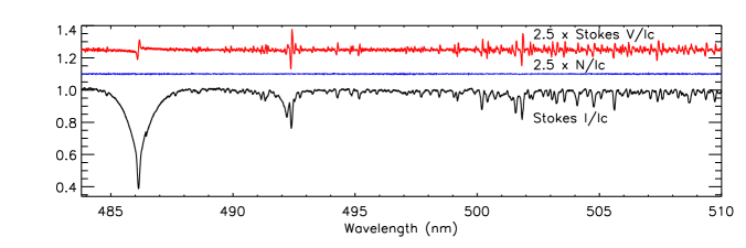
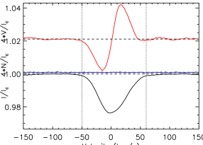
Figure 1: Left - A small region of a typical polarized spectrum acquired with the ESPaDOnS instrument during the MiMeS project. This figure illustrates the spectrum of the B5Vp magnetic He weak star HD 175362 (Wolffs’ Star), a MiMeS Targeted Component target exhibiting a peak longitudinal magnetic field of over 5 kG. From bottom to top are shown the Stokes $I$ spectrum (in black), the diagnostic null ($N$) spectrum (in blue), and the Stokes $V$ spectrum (in red). Notice the strong polarization variations across spectral lines exhibited in the Stokes $V$ spectrum. Such variations represent signatures of the presence of a strong magnetic field in the line-forming region. The simultaneous absence of any structure in the $N$ spectrum gives confidence that the Stokes $V$ detection is real, and unaffected by significant systematic effects. The $V$ and $N$ spectra have been scaled and shifted vertically for display purposes. The signal-to-noise ratio of this spectrum at 500 nm is 860 per pixel. Right - The Least-Squares Deconvolved (LSD) profiles of the full spectrum corresponding to the left panel. Again, the $V$ and $N$ spectra have been scaled and shifted vertically for display purposes. LSD profiles (described in Sect. 3) are the principal data product used for diagnosis and measurement of stellar magnetic fields in the MiMeS project. The disc averaged, line of sight (longitudinal) magnetic field measured from the Stokes $V$ profile (between the dashed integration bounds) is $4380\pm 55$ G, while for the $N$ profile it is $-3\pm 16$ G.

The Magnetism in Massive Stars (MiMeS) project is aimed at better understanding the magnetic properties of B- and O-type stars through observation, simulation, and theory. The purpose of this paper is to establish the motivation, strategy and goals of the project, to review the instrumentation and observational techniques used (§2), to describe the sample of targets that was observed and the exposure time calculations (§3), to discuss the polarimetric performance, stability and uncertainty of the instrumentation (§4), and to summarize the previous and forthcoming publications (§5).

2 Instrumentation and observations

2.1 Overview

The central focus of the observational effort of the MiMeS project has been the acquisition of high resolution broadband circular polarization (Stokes $I$ and $V$) spectroscopy. This method relies on the circular polarization induced in magnetically-split spectral line $\sigma$ components due to the longitudinal Zeeman effect (see, e.g. Mathys, 1989; Landi Degl’Innocenti & Landolfi, 2004; Donati & Landstreet, 2009; Landstreet, 2009a, b, for details concerning the physical basis of the method). Although some high resolution linear polarization (Stokes $QU$) and unpolarized spectroscopy has been acquired, the data described in this paper and those that follow in this series, will be primarily Stokes $I+V$ spectra.

High spectral resolution ($R\mathrel{\hbox{\hbox to0.0pt{\hbox{\lower 4.0pt\hbox{$\sim$}}\hss}\hbox{$>$}}}65,000$) and demonstrated polarimetric precision and stability were the principal characteristics governing the selection of instrumentation. As a consequence, the project exploited the entire global suite of suitable open-access instruments: the ESPaDOnS spectropolarimeter at the Canada-France-Hawaii Telescope (CFHT), the Narval instrument at the Télescope Bernard Lyot (TBL) at Pic du Midi observatory, and the HARPSpol instrument at ESO’s La Silla 3.6m telescope. As demonstrated in previous studies (e.g. Shultz et al., 2012; David-Uraz et al., 2014; Donati et al., 2006b), these instruments provide the capability to achieve high magnetic precision, to distinguish the detailed contributions to the complex spectra of hot stars, and to construct sophisticated models of the magnetic, chemical and brightness structures of stellar surfaces, as well as their circumstellar environments.

2.2 Observational strategy

To initiate the observational component of the MiMeS project, the collaboration was awarded a 640 hour Large Program (LP) with ESPaDOnS. This award was followed by LP allocations with Narval (137 nights, or 1213 hours), and with HARPSpol (30 nights, or 280 hours).

Some of this observing time was directed to observing known or suspected magnetic hot stars (the MiMeS Targeted Component, ‘TC’), while the remainder was applied to carrying out a broad and systematic survey of the magnetic properties of bright O and B stars (the Survey Component,‘SC’). This allowed us to obtain basic statistical information about the magnetic properties of the overall population of hot, massive stars, while also performing detailed investigations of individual magnetic massive stars. An illustration of a typical MiMeS spectrum of a magnetic TC star is provided in Fig. 1.

Most observations were further processed using the Least-Squares Deconvolution (LSD) procedure (Donati et al., 1997; Kochukhov, Makaganiuk & Piskunov, 2010). LSD is a cross-correlation multiline procedure that combines the signal from many spectral lines, increasing the effective signal-to-noise ratio (SNR) of the magnetic field measurement and yielding the highest sensitivity magnetic diagnosis available (Wade et al., 2000; Landstreet et al., 2008). The LSD procedure used in MiMeS data analysis is described in more detailed in Sect. 3.4.

Over 4800 spectropolarimetric observations of 560 stars were collected through LP and archival observations to derive the MiMeS SC and TC. Approximately 50% of the observations were obtained with Narval, 39% with ESPaDOnS and the remainder (11%) with HARPSpol. The distribution of observation acquisition with time is illustrated in Fig. 2.

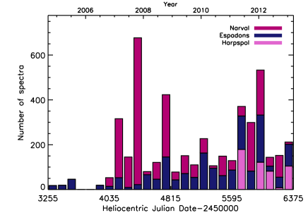
Figure 2: Distribution of data acquisition with time, showing observations acquired with individual instruments (in different colours).

2.3 ESPaDOnS

2.3.1 Instrument

ESPaDOnS - the Echelle SpectroPolarimetric Device for the Observation of Stars (e.g. Donati, 2003) - is CFHT’s optical, high resolution echelle spectrograph and spectropolarimeter. The instrument consists of a bench-mounted cross-dispersed echelle spectrograph, fibre-fed from a Cassegrain-mounted polarimeter unit. The polarimeter unit contains all instrumentation required for guiding, correction of atmospheric dispersion, calibration exposures (flat-field, arc and Fabry-Perot frames), and polarimetric analysis. It employs Fresnel rhombs as fixed quarter-wave and two rotatable half-wave retarders, and a Wollaston prism as a polarizing beamsplitter. The analyzed starlight is transported using two long optical fibres to the spectrograph, located in the CFHT’s inner coudé room, and housed in a thermal enclosure to minimize temperature and pressure fluctuations. A fibre agitator is located immediately before the entrance to the spectrograph. The role of this device is to remove modal noise present in the light transmitted through the optical fibers (Baudrand & Walker, 2001).

A tunable Bowen-Walraven image slicer slices the twin 1.6” circular images of the fiber heads at a rate of 3 slices per fiber, producing images of a pseudo-slit $\sim$12 pixels wide. The slit is tilted, resulting in sampling the pseudo-slit image in such a way that resolution is enhanced. As a consequence, the ultimate sampling of one “spectral bin” is 0.6923 “CCD bins”.

In polarimetry mode, forty spectral orders are captured in each exposure containing both polarized beams. These curved orders are traced using flat-field exposures. The images of the pseudo-slit are also tilted with respect to the detector’s rows, and the tilt is measured using Fabry-Perot exposures, which produce regularly spaced images of the pseudo-slit along each order.

2.3.2 Observations

A typical spectropolarimetric observation with ESPaDOnS captures a polarized spectrum in the Stokes $I$ and $V$ parameters with mean resolving power $R=\lambda/\Delta\lambda\sim 65\,000$, spanning the wavelength range of 369-1048 nm with 3 very small gaps: 922.4-923.4 nm, 960.8-963.6 nm, 1002.6-1007.4 nm. Spectropolarimetric observations of a target are constructed from a series of 4 individual subexposures, between which the orientation of the half-wave rhombs is changed, so as to switch the paths of the orthogonally polarized beams. This allows the removal of spurious astrophysical, instrumental and atmospheric artefacts from the polarization spectrum to first order (e.g. Donati et al., 1997). For further details on the instrument characteristics and observing procedure, see Silvester et al. (2012) and Appendix A of de la Chevrotière et al. (2013).

LP observations of MiMeS targets with ESPaDOnS were initiated in July 2008, and continued until January 2013. A total of 640 hours were allocated to the LP (see Table 1). CFHT program identifications associated with MiMeS were P13 (highest priority, about 1/3 of the time awarded) and P14 (lower priority, about 2/3 of the time awarded) prefixed by the semester ID (e.g. data acquired during semester 2010B have program ID 10BP13 and 10BP14).

CFHT observations were conducted under a Queued Service Observing (QSO) operations scheme. In this scheme, MiMeS observations were scheduled on a nightly basis, according to observability of targets, specified time constraints or monitoring frequencies, weather, and seeing conditions, in combination with observations requested by other LPs and regular observing programs, in order to optimally satisfy the observing requirements and constraints of the various programs.

Due to the particular characteristics of CFHT’s 3 primary instruments (ESPaDOnS; a wide-field, prime focus optical imager MegaCam; and a wide-field, prime focus infra-red imager WIRCam), only one instrument can be used on the telescope at a time. As a consequence, ESPaDOnS’s fibers are periodically connected and disconnected from the polarimetric module mounted on the telescope. The polarimetric module is only removed from the Cassegrain focus environment when the Adaptive Optics Bonnette is used, on average once a year, or during engineering shutdowns (e.g. for re-aluminization of the primary mirror, which occurred in Aug. 2011). During the 9 semesters of observation, ESPaDOnS’s fibers were typically dis- and re-connected 2-4 times per semester. The instrument was operational for about 40 total nights per semester. A total of 726.8 LP hours were observed and 594.2 hours were validated on 1519 spectra of 221 targets, corresponding to a validated-to-allocated ratio of 93% (see Table 1). Observations were considered to be validated when they met the specified technical requirements of the observation, typically minimum SNR and any scheduling requirements (e.g. for TC targets). However, unless unvalidated observations were patently unusable (e.g. incomplete exposure sequences, SNR too low for reduction), they were usually analysed and included in the analysis. In the case of SC targets, such observations were often one of several spectra obtained as part of a multi-observation sequence. In the case of TC targets, such observations (if of lower SNR) might still usefully contribute to sampling the phase variation of the target, or (if obtained at the wrong phase) might serve to confirm measurements obtained at other phases.

While the large majority of these spectra represent Stokes $I+V$ observations, a small number (about 120) correspond to Stokes $I+Q$ or Stokes $I+U$ (linear polarization) observations of about 10 stars.

Calibration of the instrument (bias, flat-field, wavelength calibration and Fabry-Perot exposures) uses a combination of thorium/argon and thorium/neon lamps, with all calibrations taken at the beginning or end of the night. The arc spectra are used for the primary wavelength calibration; telluric lines are then later used to fine-tune the wavelength calibration during the reduction process. Filters are used to minimise blooming on the chip at the red end of the spectrum. Two tungsten lamps are utilised for the flat field frames, with one low intensity lamp being used with a red filter and the other lamp being higher intensity and used with a blue filter. The Fabry-Perot exposure is used to fit the shape and tilt of the pseudo-slit created by the image slicer.

Approximately 85% of the ESPaDOnS data included in the SC derive from the Large Program. In addition to the LP observations, suitable public data collected with ESPaDOnS were obtained from the CFHT archive and are included in our analysis. Archival data corresponded to over 350 polarimetric spectra of about 80 additional targets obtained during engineering and Director’s time [04BD51, 04BE37, 04BE80, 06BD01] and by PIs (Catala [05AF05, 06AF07, 06BF15, 07BF14], Dougados [07BF16], Landstreet [05AC19, 07BC08], Petit [07AC10, 07BC17], Montmerle [07BF25], Wade [05AC11, 05BC17, 07AC01]). All good-quality Stokes $V$ spectra of O and B stars acquired in archival ESPaDOnS programs up to the end of semester 2012B were included.

About 50% of the included ESPaDOnS observations correspond to TC targets, and 50% to SC targets.

2.3.3 Reduction

ESPaDOnS observations are reduced by CFHT staff using the Upena pipeline feeding the Libre-ESpRIT reduction package (Donati et al., 1997), which yields calibrated $I$ and $V$ spectra (or $QU$ linear polarization spectra) of each star observed. The Libre-ESpRIT package traces the curved spectral orders and optimally extracts spectra from the tilted slit. Two diagnostic null spectra called the $N$ spectra, computed by combining the four sub-exposures in such a way as to have real polarization cancel out, are also computed by Libre-ESpRIT (see Donati et al. (1997) or Bagnulo et al. (2009) for the definition of the null spectrum). The $N$ spectra represent an important test of the system for spurious polarization signals that is applied during every ESPaDOnS spectropolarimetric observation.

The results of the reduction procedure are one-dimensional spectra in the form of ascii tables reporting the wavelength, the Stokes $I$, $V$, ($Q/U$), and $N$ fluxes, as well as a formal uncertainty, for each spectral pixel. The standard reduction also subtracts the continuum polarization, as ESPaDOnS only accurately and reliably measures polarization in spectral lines. CFHT distributes the reduced polarimetric data in the form of fits tables containing 4 versions of the reduced data: both normalized and unnormalized spectra, each with heliocentric radial velocity (RV) correction applied both using and ignoring the RV content of telluric lines. In this work we employ only the CFHT unnormalized spectra. We co-added any successive observations of a target. Then, each reduced SC spectrum was normalized order-by-order using an interactive idl tool specifically optimized to fit the continuum of these stars. The continuum normalisation is found to be very reliable in most spectral orders. However, the normalization of those orders containing Balmer lines is usually not sufficiently accurate for detailed analysis of e.g. Balmer line wings. While the quality of normalization is sufficient for the magnetic diagnosis, custom normalisation is required for more specialized analyses (e.g. Martins et al., 2015).

Archival observations were reduced and normalized in the same manner as SC spectra.

In the case of TC targets, normalization was often customized to the requirements of the investigation of each star. This is also the case for stars or stellar classes with unusual spectra, such as WR stars (e.g. de la Chevrotière et al., 2014).

All CFHT ESPaDOnS data, including MiMeS data and archival data discussed above, can be accessed in raw and reduced form through general queries of the CFHT Science Archive via the Canadian Astronomy Data Centre (CADC). The PolarBase archive also hosts an independent archive of most raw and reduced data obtained with ESPaDOnS.

2.3.4 Issues

During the 4.5-year term of the LP, two activities have occurred at the observatory that are important in the context of the MiMeS observations.

Identification and elimination of significant ESPaDOnS polarimetric crosstalk:  During the commissioning of ESPaDOnS in 2004 it was found that the instrument exhibited crosstalk between linear polarization and circular polarization (and vice versa). Systematic investigation of this problem resulted in the replacement of the instrument’s atmospheric dispersion corrector (ADC) in the fall of 2009, reducing the crosstalk below 1%. Periodic monitoring of the crosstalk confirms that it has remained stable since 2009. However, higher crosstalk levels were likely present (with levels as high as 5%) during the first 3 semesters of MiMeS LP observations. The absence of any significant impact of crosstalk on most MiMeS observations is confirmed through long-term monitoring of TC targets as standards, and is addressed in §4.2. The crosstalk evolution and mitigation is described in more detail by Barrick, Benedict & Sabin (2010) and Silvester et al. (2012).

Change of the ESPaDOnS CCD: Until semester 2011A, ESPaDOnS employed a grade 1 EEV CCD42-90-1-941 detector with 2K x 4.5K 0.0135 mm square pixels (known as EEV1 at CFHT). This was replaced in 2011A with a new deep-depletion E2V CCD42-90-1-B32 detector (named Olapa). Olapa has exquisite cosmetics and much less red fringing than EEV1. Another major difference is that Olapa’s quantum efficiency in the red is about twice as high as with EEV1. Commissioning experiments by CFHT staff, as well as within the MiMeS project, were used to confirm that observations acquired before and after the CCD replacement are in excellent agreement. This is discussed further in §4.2.

Table 1: ESPaDOnS observations 2008B-2012B. “Validated” observations are deemed by the observatory to meet stated SNR, scheduling and other technical requirements. Sometimes, due to observatory QSO requirements, more hours were observed than were actually allocated. This potentially produced ratios of validated-to-allocated time (Val/Alloc) greater than 100%.

ID	Allocated	Observed	Validated	Val/Alloc
	(h)	(h)	(h)	(%)
08BP13	25.5	19.8	16.5	65
08BP14	61.6	65.5	57	93
09AP13	28	16.9	15.7	56
09AP14	43	36.2	34.2	80
09BP13	22	31.2	21.9	100
09BP14	34.1	43.2	33.9	99
10AP13	28	32.7	26.4	94
10AP14	43	51.6	42.8	100
10BP13	24	29.7	26.6	111
10BP14	36	38.8	34.6	96
11AP13	28	29.7	25.5	91
11AP14	43.3	48.7	38.4	89
11BP13	28	23.6	22.7	81
11BP14	43.3	47.8	38.3	88
12AP13	25	29.7	27.8	111
12AP14	46.3	53.7	52.7	114
12BP13	24.9	54.8	31.3	126
12BP14	56	73.2	47.9	86
Total	640	726.8	594.2	93

2.4 Narval

2.4.1 Instrument

Narval is a near-twin of ESPaDOnS installed at the 2m Télescope Bernard Lyot (TBL) in the French Pyrénées. It is composed of a Cassegrain polarimeter unit similar to that of ESPaDOnS, and a similar spectrograph located in the TBL coudé room.

Compared to ESPaDOnS, the instrument was only adapted to the smaller telescope size. Small differences include the diameter of the entrance pinhole of the Cassegrain unit (2.8” for Narval, versus 1.6” for ESPaDOnS) and the lack of a fibre agitator. However, the sampling of the (sliced) pinhole image is identical to that of ESPaDOnS. The CCD used at TBL (a back illuminated e2v CCD42-90 with $13.5\mu$m pixels) differs from that used at CFHT. However, each Narval spectrum also captures 40 spectral orders covering a similar spectral range (370-1050 nm) with the same resolving power of about 65 000.

All other technical characteristics of Narval are effectively identical to those of ESPaDOnS described in Sect 2.3.1.

2.4.2 Observations

Observations of MiMeS targets with Narval were initiated in March 2009, and continued until January 2013. A total of 1213 hours were allocated to the MiMeS program, first in the framework of 3 single-semester programs and then as an LP for 5 additional semesters (all of these observations are hereinafter considered to be ’LP’ observations). TBL program identifications associated with MiMeS were prefixed by the letter ”L”, followed by the year (e.g. ”12” for 2012) and the semester (1 or 2 for semesters A and B, respectively), then ”N” for Narval, and the ID of the program itself (e.g. ”02” in the case of the LP). The MiMeS Narval runs are thus L091N02, L092N06, L101N11, L102N02, L111N02, L112N02, L121N02 and L122N02.

Just like at CFHT, TBL observations are conducted under a QSO operations scheme. The difference, however, is that Narval is the only instrument available at TBL and thus stays mounted on the telescope all of the time and Narval observations can occur on any night (except during technical maintenance periods or closing periods). Calibration spectra (bias, flat-field, wavelength calibration) are obtained at both the beginning and end of each observing night.

In total, 1213 hours were allocated and 564.5 hours were validated on approximately 890 polarimetric observations of about 35 targets, corresponding to a validated-to-allocated ratio of 46.5% (see Table 2). Observations were only validated when they met the requirements of the program: observations were generally not validated when taken under very poor sky conditions or when the requested observing phase was not met. While the large majority of these spectra represent Stokes $I+V$ observations, a small number (about 20) correspond to Stokes $I+Q$ or Stokes $I+U$ (linear polarization) observations of one star (HD 37776).

In addition to the MiMeS observations, suitable public data acquired with Narval were obtained from the TBL archive and are included in our analysis. Archival data corresponded to over 1550 polarimetric spectra of about 60 additional targets (PIs Alecian [L071N03, L072N07, L081N02, L082N11, L091N01, L092N07], Bouret [L072N05, L081N09, L082N05, L091N13], Henrichs [L072N02], Neiner [L062N02, L062N05, L062N07, L071N07, L072N08, L072N09, L081N08]).

About 550 of the included Narval observations correspond to TC targets (i.e. about 22%), and the remainder to SC targets.

Approximately 35% of the Narval data included in the SC derive from the Large Program or the dedicated single-semester programs summarized in Table 2.

All TBL Narval data, including MiMeS data and archival data discussed above, can be accessed in raw and reduced form through general queries of the TBL Narval Archive. Most observations are also available through PolarBase⁶.

2.4.3 Reduction

Similarly to the ESPaDOnS observations, Narval data were reduced at the observatory using the Libre-ESpRIT reduction package. TBL distributes the reduced polarimetric data in the form of ascii tables containing either normalized or unnormalized spectra, with heliocentric radial velocity (RV) correction applied both using and ignoring the RV content of telluric lines. As with the ESPaDOnS data, for SC (and PI) targets we used unnormalized spectra, co-added any successive observations of a target, and normalized them order-by-order using an interactive idl tool specifically optimized to fit the continuum of hot stars.

2.4.4 Issues

During the 4-year term of the MiMeS Narval observations, two technical events occurred at TBL that are important in the context of the project.

CCD controller issue: From September 23, 2011 to October 4, 2011, abnormally high noise levels were measured in the data. This was due to an issue with an electronic card in the CCD controller. The controller was replaced on October 4 and the noise returned to normal.

Loss of reference of a Fresnel rhomb: In the summers of 2011 and 2012, a loss of positional reference of Fresnel rhomb #2 of Narval was diagnosed. This happened randomly but only at high airmass and high dome temperature. In 2011 the position was only slightly shifted and resulted in a small decrease in the amplitude of Stokes $V$ signatures. In 2012 however, the error in position was sometimes larger and resulted in distorted Stokes $V$ signatures. This technical problem certainly occurred in 2012 on July 12, 15 to 19, and September 4, 7, 11, and 14. It probably also occurred in 2011 on August 17, 18, 20 to 22, and in 2012 on July 8 to 11, 22 to 24, August 18 to 20, and September 5, 6 and 8. The rest of the MiMeS data collected in the summers of 2011 and 2012 appear to be unaffected. Note that this technical problem cannot create spurious magnetic signatures, but could decrease our ability to detect weak signatures and does forbid the quantitative interpretation of magnetic signatures in terms of field strength and configuration.

Since both of these problems were discovered following data acquisition, MiMeS observations obtained during periods affected by these issues were generally validated, and appear as such in Table 2.

Table 2: Narval observations 2009A-2012B. Observed and validated times include CCD readout times. “Validated” observations are deemed by the observatory to meet stated SNR, scheduling and other technical requirements. Sometimes, due to observatory QSO requirements, more hours were observed than were actually allocated. This sometimes produced ratios of validated-to-allocated time greater than 100%.The conversion from nights to hours at TBL has changed with time: for summer nights it was 9h/n in 2009 and 2010 and then $\sim$7h/n in 2011 and 2012; for winter nights it went from 11h/n in 2009, to $\sim$10h/n in 2010 and then 8h/n in 2011 and 2012.

ID	Allocated		Observed	Validated	Val/Alloc
	(n)	(h)	(h)	(h)	(%)
L091N02	24	216	27.2	27.2	12.6
L092N06	24	264	54.0	49.9	18.9
L101N11	24	216	27.7	27.7	12.8
L102N02	13	129	112.0	100.8	78.1
L111N02	13	90	100.1	94.5	105.0
L112N02	13	104	101.3	87.2	83.9
L121N02	13	90	97.3	95.5	106.1
L122N02	13	104	86.7	82.6	79.5
Total	137	1213	605.3	564.5	46.5

2.5 HARPSpol

2.5.1 Instrument

We also used the HARPSpol (Piskunov et al., 2011) polarimetric mode of the HARPS spectrograph (Mayor et al., 2003) installed on the 3.6m ESO telescope (La Silla Observatory, Chile). The polarimetric module has been integrated into the Cassegrain unit situated below the primary mirror. As with ESPaDOnS and Narval, the Cassegrain unit provides guiding and calibration facilities, and feeds both fibres of HARPS with light of orthogonal polarization states. The polarimeter comprises two sets of polarization optics that can slide on a horizontal rail. Each set of polarimetric optics consists of a polarizing beamsplitter (a modified Glan-Thompson prism) and a rotating super-achromatic half-wave (for linear polarization) or quarter-wave (for circular polarization) plate that converts the polarization of the incoming light into the reference polarization of the beamsplitter. The light beams are injected into fibres of diameter 1” on the sky, which produce images 3.4 pixels in diameter. They feed the spectrograph installed in a high stability vacuum chamber in the telescope’s coudé room. The spectra are recorded on a mosaic of two 2k$\times$4k EEV CCDs, and are divided into 71 orders (45 on the lower, blue, CCD, and 26 on the upper, red, CCD).

2.5.2 Observations

A typical polarimetric measurement provides simultaneous Stokes $I$ and $V$ echelle spectra with a mean resolving power of $110\,000$, covering a wavelength range from 380 to 690 nm, with a gap between 526 and 534 nm (separating both CCDs). As with ESPaDOnS and Narval, a single polarization measurement is constructed using 4 successive subexposures between which the quarter-wave plate is rotated by 90^∘ starting at 45^∘ (for circular polarization). The calibration spectra (bias, tungsten flat-field, and ThAr wavelength calibration) are systematically obtained at the beginning of each observing night, and in many cases at the end of the night as well.

Table 3: HARPSpol observations during the periods P87-P91. Columns indicate the run ID, run dates, period ID, the number of allocated nights, the estimated number of equivalent operational hours, and the fraction of time useful for observations.

run ID	Dates	P	Nights	Hrs	Obs
(187.D-)	(local time)				time (%)
0917(A)	2011 May 21-27	87	7	70	67
0917(B)	2011 Dec 9-16	88	8	64	100
0917(C)	2012 Jul 13- Aug 1	89	7	70	52
0917(D)	2013 Feb 13-20	90	8	64	93
0917(E)	2013 Jun 20	91	1	10	100
Total			31	278	80

Figure 3: Distribution of $V$ band apparent magnitudes of all observed SC targets.

Unlike ESPaDOnS and Narval, HARPSpol is scheduled using a classical scheduling model, in “visitor” mode. The HARPSpol observations of the MiMeS project were obtained in the framework of Large Program 187.D-0917 over 5 semesters (Periods 87-91, March 2011-September 2013). A total of 30 nights were initially allocated. We obtained one additional night at the end of the project to compensate for bad weather conditions. The observations were obtained during 5 runs, one per Period lasting 1, 7 or 8 nights (Table 3). In July 2012 we shared the nights allocated to our run with two other programs, scheduled between July 13th and August 1st. This gave us the possibility to monitor objects with relatively long rotation periods, over more than 7 days, and up to 20 days, allowing us to sample the rotation cycles of TC targets. A total of 532 individual polarized spectra, resulting in 266 coadded observations of 173 stars, were obtained during this LP. All observations were obtained in circular polarization (Stokes $V$) mode.

All HARPSpol data, including MiMeS data discussed above, can be accessed in raw form through general queries of the ESO Science Archive.

2.5.3 Reduction

The data were reduced using the standard reduce package (Piskunov & Valenti, 2002) which performs an optimal extraction of the cross-dispersed echelle spectra after bias subtraction, flat-fielding correction (at which stage the echelle ripple is corrected), and cosmic ray removal. Additionally, we used a set of proprietary idl routines developed by O. Kochukhov to perform continuum normalisation, cosmic ray cleaning, and polarimetric demodulation (e.g. Alecian et al., 2011; Makaganiuk et al., 2011).

The optimally extracted spectra were normalized to the continuum following two successive steps. First, the spectra were corrected for the global response function of the CCD using a heavily smoothed ratio of the solar spectrum measured with HARPSpol, divided by Kurucz’s solar flux atlas (Kurucz et al., 1984). The response function corrects the overall wavelength-dependent optical efficiency of the system, the CCD sensitivity (which varies smoothly with wavelength), and also the flux distribution of the flat-field lamp. The latter is not smooth because the HARPS flat-field lamp uses filters to suppress the red part of the spectrum. Then we determined the continuum level by iterative fitting of a smooth, slowly varying function to the envelope of the entire spectrum. Before this final step we carefully inspected each spectrum and removed the strongest and broadest lines (including all Balmer lines, and the strongest He lines), as well as the emission lines, from the fitting procedure.

The polarized spectra and diagnostic null were obtained by combining the four continuum-normalized individual spectra taken at the four different angles of the wave-plate, using the ratio method (Donati et al., 1997). The spectra of both CCDs, up to this point reduced independently, are then merged to provide a single full spectrum. The heliocentric velocity corrections were computed for the four spectra, and the mean of the four values was applied to Stokes $I$ and $V$, as well as diagnostic null spectra. If successive polarimetric measurements of the same object were obtained, we combined them using a SNR-weighted mean. Each reduced observation was then converted into an ascii file in the same format as Narval data.

All of the HARPSpol data included in the SC derive from the LP, since when the LP was completed no significant archival HARPSpol data existed that were suitable to our purposes.

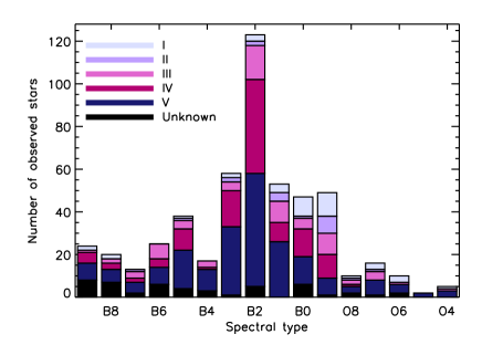
Figure 4: Distribution of spectral types and luminosity classes of all observed SC targets, excluding the WR stars, which are discussed in detail by de la Chevrotière et al. (2014).

2.6 Complementary observations

In addition to the spectropolarimetric data described above, significant complementary data were also acquired, principally in support of the TC. Some of these data were archival in nature (e.g. IUE spectroscopy, Hipparcos photometry, XMM-Newton and Chandra data). Some were acquired through other projects or surveys (e.g. the GOSSS, NoMaDs and OWN surveys, Sota et al., 2011; Maíz Apellániz et al., 2012; Barbá et al., 2010) and graciously shared with the MiMeS project through collaborative relationships (e.g. Wade et al., 2012b). Other data were obtained specifically in support of the MiMeS project: additional Stokes $V$ spectropolarimetry obtained with FORS2, dimaPol and SemPol (e.g. Grunhut et al., 2012a; Henrichs et al., 2012), high resolution optical spectroscopy obtained with the FEROS and UVES spectrographs (e.g. Grunhut et al., 2012a; Wade et al., 2012b; Shultz et al., 2015), ultraviolet spectroscopy obtained with the Hubble Space Telescope’s STIS spectrograph (e.g. Marcolino et al., 2013), X-ray spectroscopy obtained with the XMM-Newton and Chandra X-ray telescopes (e.g. Nazé et al., 2014; Petit et al., 2015), high precision optical photometry obtained with the MOST space telescope (Grunhut et al., 2012a), optical phase interferometry obtained with the VLTI (Rivinius et al., 2012), optical broadband linear polarization measurements obtained using the IAGPOL polarimeter on the 0.6m telescope of the Pico dos Dias Observatory (e.g. Carciofi et al., 2013), and low frequency radio flux measurements (Chandra et al., 2015).

The details of these observations are described in the respective associated publications.

3 Targets and exposure times

Table 4: MiMeS Targeted Component (TC) sample (32 stars observed, 30 with detected magnetic fields). In addition to HD # and secondary identifier, we provide the spectral type (typically obtained from the Bright Star Catalogue (Hoffleit & Jaschek, 1991), the # of observations acquired and the instruments used (Inst; E=ESPaDOnS, N=Narval, H=HARPSpol), the magnetic field detection status (Det?; T=True, F=False), a reference to completed MiMeS publications, the approximate rotational period, and the peak measured longitudinal field strength. For some TC targets (indicated with a $\dagger$ beside their number of observations), observations include Stokes $Q$/$U$ spectra in addition to Stokes $V$ spectra.

HD	Other ID	Spectral	# obs	Inst	Det?	Reference	$P_{\rm rot}$	$|\langle B_{z}\rangle_{\rm max}|$
		Type					(d)	(G)
	BD-13 4937	B1.5 V	31	EN	T	Alecian et al. (2008b)		$1390\pm 395$
3360	$\zeta$ Cas	B2 IV	97	N	T	Briquet et al. (to be submitted)	5.37	$30\pm 5$
34452	IQ Aur	A0p	40	N	T		2.47	$1080\pm 310$
35502		B5 V + A + A	21	EN	T		0.85	$2345\pm 245$
36485	$\delta$ Ori C	B2 V	10	N	T		1.48	$2460\pm 85$
36982	LP Ori	B0 V	15	EN	T	Petit et al. (2008)	2.17	$220\pm 50$
37017	V1046 Ori	B1.5 V	10	E	T		0.90	$2035\pm 1075$
37022	$\theta^{1}$ Ori C	O7 V p	30	E	T		$15.42$	$590\pm 115$
37061	NU Ori	B4	17	E	T	Petit et al. (2008)	0.63	$310\pm 50$
37479	$\sigma$ Ori E	B2 V p	18	NE	T	Oksala et al. (2012)	1.19	$2345\pm 55$
37490	$\omega$ Ori	B3 III e	121	NE	F	Neiner et al. (2012b)	1.37	$\mathrel{\hbox{\hbox to0.0pt{\hbox{\lower 4.0pt\hbox{$\sim$}}\hss}\hbox{$<$}}}90$
37742	$\zeta$ Ori A	O9.5 Ib	495	N	T	Blazère et al. (2015)	7.0	$55\pm 15$
37776	V901 Ori	B2 V	77$\dagger$	EN	T		1.54	$1310\pm 65$
47777	HD 47777	B0.7 IV-V	10	E	T	Fossati et al. (2014)	2.64	$470\pm 85$
50896	EZ CMa	WN4b	92$\dagger$	E	F	de la Chevrotière et al. (2013)	3.77	$\mathrel{\hbox{\hbox to0.0pt{\hbox{\lower 4.0pt\hbox{$\sim$}}\hss}\hbox{$<$}}}50$
64740	HD 64740	B1.5 V p	17	HE	T		1.33	$660\pm 60$
66522	HD 66522	B1.5 III n	4	H	T			$610\pm 15$
79158	36 Lyn	B8 III pMn	29	N	T		3.84	$875\pm 70$
96446	V430 Car	B2 IV/V	10	H	T	Neiner et al. (2012c)	0.85	$2140\pm 270$
101412	V1052 Cen	B0.5 V	7	H	T		42.08	$785\pm 55$
124224	CU Vir	Bp Si	24	EN	T	Kochukhov et al. (2014)	0.52	$940\pm 90$
125823	a Cen	B7 III pv	26	EH	T		8.82	$470\pm 15$
133880	HR Lup	B8IVp Si 4200	2	E	T	Bailey et al. (2012)	0.88	$4440\pm 160$
149438	$\tau$ Sco	B0 V	12	E	T		41.03	$90\pm 5$
163472	V2052 Oph	B2 IV-V	44	N	T	Neiner et al. (2012a)	3.64	$125\pm 20$
175362	V686 CrA	B5 V p	64$\dagger$	E	T		3.67	$5230\pm 380$
184927	V1671 Cyg	B0.5 IV nn	35$\dagger$	E	T	Yakunin et al. (2015)	9.53	$1215\pm 20$
191612		O8 f?p var	21	EN	T	Wade et al. (2011)	537	$585\pm 80$
200775	V380 Cep	B9	63	NE	T	Alecian et al. (2008a)	4.33	$405\pm 80$
205021	$\beta$ Cep	B1 IV	60	NE	T		12.00	$110\pm 5$
208057	16 Peg	B3 V e	60	NE	T		1.37	$210\pm 50$
259135	BD+04 1299	HBe	8	EN	T	Alecian et al. (2008b)		$550\pm 70$

3.1 Targeted Component

The Targeted Component (TC) was developed to provide high-quality spectropolarimetric data to map the magnetic fields and investigate related phenomena and physical characteristics of a sample of magnetic stars of great interest, at the highest level of sophistication possible for each star. Thirty-two TC targets were identified to allow the investigation of a variety of physical phenomena. The TC sample (summarized in Table 4) consists of stars that were established or suspected to be magnetic at the beginning of the project. The majority of these stars are confirmed periodic variables with periods ranging from approximately 1 d to 1.5 years, with the majority having a period of less than 10 days so that they are suitable candidates for observational monitoring and mapping. They are established to have, or show evidence for, organized surface magnetic fields with measured longitudinal field strengths of tens to thousands of gauss. These targets were typically observed over many semesters, gradually building up phase coverage according to their periods and the operation schedule of the respective instruments. The strict periodicity required for such an observing strategy represents an assumption capable of being tested by the data; this is described in more detail in §4. Depending on the level of sophistication of the planned analysis (which itself is a function of the limiting quality of the data and individual stellar and magnetic field properties) typically 10-25 observations were acquired for individual TC targets. For a small number of targets, linear polarization Stokes $Q$ and $U$ spectra were also acquired. While the monitoring of the majority of individual TC targets was carried out with a single instrument, for some targets a significant number of observations was acquired with multiple instruments. For example, HD 37940 ($\omega$ Ori; Neiner et al., 2012b) and HD 37776 (Landstreet’s star; Shultz et al., in prep., Kochukhov et al., in prep.) were extensively observed using both ESPaDOnS and Narval. For some TC targets, only a small number of observations was acquired, either because the target was found to be non-magnetic, non-variable or poorly suited to detailed modelling.

Overall, somewhat less than half of the LP observing time was devoted to observations of the TC. It should be noted that TC targets are the focus of dedicated papers, and are discussed here only for completeness and as a comparison sample.

Figure 5: Completeness of the SC sample as a function of apparent magnitude, to $V=8.0$. This figure illustrates the number of stars observed in the MiMeS survey versus the total number of OB stars of apparent magnitude $V<8.0$, as catalogued by simbad (Wenger et al., 2000).

Figure 6: Completeness of the sample as a function of spectral type for stars with $V<8.0$. This figure (which excludes the WR stars, which are discussed in detail by de la Chevrotière et al., 2014) illustrates the number of stars observed in the MiMeS survey versus the total number of stars of a given spectral type with apparent magnitudes brighter than $V=8.0$.

3.2 Survey Component

The Survey Component (SC) was developed to provide critical missing information about field incidence and statistical field properties for a much larger sample of massive stars, and to provide a broader physical context for interpretation of the results of the TC. Principal aims of the SC investigation are to measure the bulk incidence of magnetic massive stars, estimate the variation of field incidence with quantities such as spectral type and mass, estimate the dependence of incidence on age, environment and binarity, sample the distribution of field strengths and geometries, and derive the general statistical relationships between magnetic field properties and spectral characteristics, X-ray emission, wind properties, rotation, variability and surface chemistry diagnostics.

The SC sample is best described as an incomplete, principally magnitude-limited stellar sample. The sample is comprised of two groups of stars, selected in different ways. About 80% of the sample correspond to stars that were observed in the context of the LPs. These stars were broadly selected for sensitivity to surface magnetic fields, hence brighter stars with lower projected rotational velocities were prioritized. To identify this sample, we started from the list of all stars with spectral types earlier than B4 in the simbad database. Each target was assigned a priority score according to their apparent magnitude (higher score for brighter stars), $v\sin i$ (higher score for stars with $v\sin i$ below 150 km/s), special observational or physical characteristics (e.g. Be stars, pulsating variables, stars in open clusters) and the existence of UV spectral data, e.g. from the International Ultraviolet Explorer (IUE) archive. These targets were the subject of specific exposure time calculations according to the exposure time model described below. Spectra of the remaining 20% of the sample were retrieved from the ESPaDOnS and Narval archives. These spectra, corresponding to all stars of spectral types O and B present in the archives at the end of the LPs, were acquired within the context of various programs (generally) unrelated to the MiMeS project (see Sects. 2.3.2 and 2.4.2).

3.3 Properties of observed sample

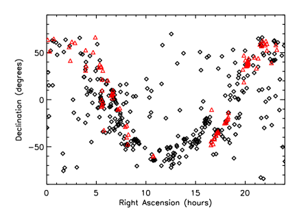
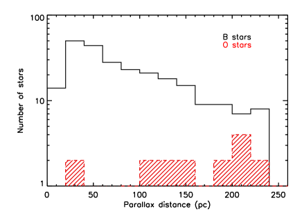
Figure 7: Left - Location of all O-type (red triangles) and B-type (black diamonds) SC targets as a function of right ascension and declination. Right - Histogram illustrating distances to the 267 SC stars having high quality ($\pi/\sigma_{\pi}>4$) measured Hipparcos parallaxes.

A total of 560 distinct stars or stellar systems were observed (some with more than one instrument), of which 32 were TC targets. Of the 528 SC targets, 106 were O stars or WR stars, and 422 were B stars. Roughly 50% of the targets were observed with ESPaDOnS, 17% with Narval and the remaining 33% with HARPSpol.

We emphasize that our selection process was based on spectral types and motivated by our principal aim: to build a suitable sample to study both the statistics of fossil fields in high-mass stars, and the various impacts of magnetic fields on stellar structure, environment and evolution.

Within this sample, significant subsamples of O and B supergiants, Oe/Be stars and pulsating B stars exist. A systematic survey of the O and B star members of 7 open clusters and OB associations of various ages was also conducted, in order to investigate the temporal evolution of magnetic fields. The cluster sample was selected to include clusters containing very young ($\sim 5$ Myr) to relatively evolved ($\sim 100$ Myr) O and B type stars. These subsamples will be the subjects of dedicated analyses (see §5).

Fig. 3 shows that the distribution of apparent magnitude of the sample peaks between 4.5 and 7.5 (the median $V$ magnitude of the sample is 6.2), with an extended tail to stars as faint as 13.6.

The distributions of $V$ magnitude, spectral type and luminosity class of the SC sample are illustrated in Figs. 3 and 4, respectively. Approximately 6180 stars of spectral types O and B with apparent magnitudes $V$ brighter than $8.0$ are included in the simbad database (Wenger et al., 2000); the MiMeS project observed or collected observations of 410 stars brighter than this threshold. Thus overall, we observed about 7% of the brightest O and B stars. Within this magnitude range, the brightest stars were observed preferentially; for example, 50% of O and B stars brighter than $V=4$ are included in the sample, and a little more than 20% of O and B stars brighter than $V=6$ are included. The completeness of the sample as a function of apparent magnitude is illustrated in Fig. 5.

Although the initial survey excluded stars with spectral types later than B3, Fig. 4 shows that with the inclusion of archival data and due to reclassification of some of our original targets, a significant number of later B-type stars (about 140) form part of the analyzed sample. Including these cooler stars is valuable, since it helps to bridge the gap with the statistics known at later spectral types (F5-B8; e.g. Wolff, 1968; Power et al., 2008) and to understand the uncertainties on the spectral types, especially for chemically peculiar stars, for which chemical peculiarities could lead to inaccurate inference of the effective temperature. The strong peak at spectral types B2-B3 reflects the natural frequency of this classification (see, e.g. Hoffleit & Jaschek, 1991). Spectral types up to O4, as well as a dozen WR stars, are included in the sample. The large majority of SC targets (about 70%) are main sequence (i.e. luminosity class V and IV) stars. Of the evolved targets, 15% are giants (class III), 5% are bright giants (class II) and 10% are supergiants (class I).

The MiMeS sample preferentially included stars with earlier spectral types. Numerically, the most prominent spectral type observed in the survey was B2 (see Fig. 4). However, as a fraction of all stars brighter than $V=8$, the most complete spectral type was O4 (at 5/7 stars, for 71%) followed by O7 (at 16/33, for 49%). Between spectral types of B3 and O4, we observed just under one-quarter (23%) of all stars in the sky with $V<8$. The completeness as a function of spectral type is illustrated in Fig. 6.

To characterize the spatial distribution of the SC targets, we use their equatorial coordinates along with distances for those stars with good-quality parallax measurements. As could be expected, the SC sample is confined primarily to the Galactic plane, as illustrated in Fig. 7 (left panel). All of the O-type stars are located in, or close to, the Galactic plane. A majority ($\sim 85$%) of the B-type stars are located close to the Galactic plane. However, a fraction (about 15%) of the B-type targets are located well away from the plane of the Galaxy.

We have computed distances to all stars with measured Hipparcos parallaxes significant to $4\sigma$. Amongst the 106 O-type SC stars, only 19 stars have parallaxes measured to this precision. The B-type SC sample of 422 stars, on the other hand, contains 248 stars with precise parallaxes. About 140 of the B stars (more than 1/2 of those with precisely-known parallaxes) are located within 80 pc of the Sun. Approximately one-half of the SC targets have precisely determined parallax distances, and are located within about 250 pc of the Sun. The other half of the sample have poorly determined parallax distances. Overall, it can be concluded that the B-type sample is largely local, whereas the O-type sample is distributed over a larger (but poorly characterized) volume. The distributions of SC target distances are illustrated in Fig. 7 (right panel).

As a consequence of the various origins, complicated selection process and diverse properties of the stars included in the SC, the MiMeS sample is statistically complex. An understanding of the ability of the SC to allow broader conclusions to be drawn about the component subsamples will require a careful examination of the statistical properties. This will be the subject of forthcoming papers.

The details of individual stars included in the MiMeS SC sample are reported in Tables 5 and 7. Johnson $V$ magnitudes are from the simbad database (Wenger et al., 2000). Spectral types for all stars in Tables 5 and 7 were obtained from classifications published in the literature or from secondary sources (e.g. estimated from effective temperatures) when unavailable. All sources are cited in the respective tables.

Targets of the SC sample detected as magnetic were normally scheduled for systematic monitoring, in the same manner as performed for the TC targets. Many such stars have been the subjects of dedicated analyses published in the refereed literature (see §5).

3.4 Least-Squares Deconvolution

The basic data product employed to evaluate the presence or absence of a magnetic field, and to characterize the field strength or its upper limit, were Stokes $I$, $V$ and diagnostic null $N$ LSD profiles. LSD was applied to all LP and archival spectra, except those of the WR stars (see de la Chevrotière et al., 2013, 2014, for more information concerning analysis of WR stars). LSD (see Donati et al., 1997) is a multiline deconvolution method that models the stellar Stokes $I$ and $V$ spectra as the convolution of a mean profile (often called the “LSD profile”) with a line mask describing the wavelengths, unbroadened depths and Landé factors of lines occurring in the star’s spectrum. The MiMeS LSD procedure involved development of custom line masks optimized for each star, using spectral line data acquired using extract stellar requests to the Vienna Atomic Line Database (VALD; Piskunov et al., 1995). The LSD codes of both Donati et al. (1997) and Kochukhov, Makaganiuk & Piskunov (2010) were normally employed to extract mean profiles. The principal advantage of LSD is that it provides a single set of pseudo line profiles characterizing each spectrum, coherently combining the signal contained in many spectral lines. This yields an easily interpreted, high precision diagnosis of the stellar magnetic field.

The details of the LSD analysis as applied to particular subsamples of the SC and TC are described in published and forthcoming papers.

Figure 8: Illustration of exposure model predictions for dipolar magnetic fields. Left - Predicted longitudinal magnetic field formal uncertainty versus projected rotational velocity, for 4 different SNRs of the LSD profile (2500, 5000, 10000 and 20000). The model predicts a $\sim 50$ G error bar at 100 km/s for an LSD SNR of 10000. Right - Reduced $\chi^{2}$ of Stokes $V$ within the bounds of the line profile versus $v\sin i$, as a function of surface dipole polar field strength for an LSD profile SNR of 10000. The dashed line indicates the reduced $\chi^{2}$ corresponding to a detection at 99.999% confidence (i.e. a definite detection according to the criteria of Donati et al., 1997). The weakest fields are detectable only in those stars with relatively sharp lines (e.g. $v\sin i\leq 40$ km/s for 100 G, at this LSD SNR), whereas only stronger fields are detectable in rapidly rotating stars (e.g. 1 kG fields are detectable in stars with $v\sin i\leq 120$ km/s, at this LSD SNR). Different colours and linestyles are used to distinguish the various models.

Figure 9: Multiplicative gain in SNR versus spectral type assumed in the MiMeS exposure time model.

3.5 Exposure durations and time budget

LP exposure times were estimated in several ways, as follows.

For TC stars, exposure times typically were based on known amplitudes of Stokes $V$ (or $Q$/$U$) signatures, or estimated based on published field strengths and spectral characteristics. For those TC targets identified as potentially suitable for modelling using individual spectral line Stokes $IV$/$IVQU$ profiles, SNRs per spectral pixel in the reduced spectrum greater than 500 were normally desired.

The exposure times for SC targets observed within the context of the LPs were computed so as to achieve SNRs corresponding to particular levels of magnetic sensitivity. For the purposes of the survey, “magnetic sensitivity” was defined in terms of the weakest surface dipole field strength likely to be detected in a particular observation. Such an estimate is rather challenging to make, since it is a function not only of the observational parameters of a star (apparent magnitude, spectral type, line width), but also of the geometry of the surface magnetic field, as well as the assumed rotational phase at the time of observation (e.g. Petit & Wade, 2012). Our approach was based on the results of simulations in which Stokes $V$ LSD profiles of a single representative spectral line (selected to be representative of an LSD profile) were synthesized (using the Zeeman code; Landstreet, 1988; Wade et al., 2001) for a large grid of line parameters (depth, $v\sin i$), field geometries and noise levels, with the ultimate aim of deriving an estimate of sensitivity as a function of SNR and $v\sin i$. For some targets no $v\sin i$ was available, and in these cases we assumed a nominal $v\sin i$ of 150 km/s. Illustrative results of these calculations are shown in Fig. 8.

Because the number of spectral lines present in the stellar spectrum varies significantly with spectral type, the multiplex advantage offered by LSD is also a strong function of this quantity. To quantify the improvement in magnetic precision resulting from LSD, we employed existing spectra of magnetic and non-magnetic stars to estimate the multiplicative gain in SNR $G({\rm ST})$ achieved by application of LSD as a function of spectral type (ST). The gain factor is approximate, with significant variation at each spectral type depending on individual stellar spectral properties. Typically, gain factors exhibit greatest uncertainty at earlier spectral types. A quantitative evaluation of the estimated gain factors, and the overall accuracy of the exposure time model, will be presented in future papers. The gain factors employed in the exposure time calculations are illustrated in Fig. 9.

In order to detect the field strengths of interest ($\sim 100-1000$ G), very high SNRs, of order 10000 per spectral pixel in the Stokes $V$ spectrum, were required. Such high SNRs are achievable in two ways: either by co-addition of a series of deep exposures, or by line co-addition using LSD. Often, both of these approaches were combined in order to reach the desired sensitivity.

Ultimately, surface dipole sensitivity bins of $B_{\rm d}=100,$ 250, 500 G and 1 kG were adopted for the LP survey targets, based principally on published reports of the magnetic strengths of known B- and O-type stars. We implicitly assumed that very strong magnetic fields (with $B_{\rm d}\gg 1$ kG) would be quite rare, whereas weaker fields could be more numerous.

For each star in a given sensitivity bin, the exposure time was adjusted to achieve a SNR_LSD following application of LSD that allowed the detection of that field strength. For practical purposes, targets were typically assigned to the most sensitive bin for which the required exposure time for that star was below about 2 hours. Consequently, for some targets nominally assigned to the 1 kG bin the required SNR was not achievable within this practical time limit. As a result, about 25% of the LP observations (corresponding to about 90 targets) yield predicted dipole field strength sensitivities that are larger than 1 kG (Fig. 10, left frame).

The approximate relations governing the spectrum SNR required to reach a magnetic precision $B_{\rm 0.1}$ in units of 0.1 kG were determined through empirical fits to the model results:

$${\rm SNR_{\rm LSD}}=(120+170\times v\sin i)\,B_{\rm 0.1}^{-1}\ \ [{\rm if}\ v\sin i\leq 40~{}{\rm km/s}];$$ (1)

or

$${\rm SNR_{\rm LSD}}=(-18700+640\times v\sin i)\,B_{\rm 0.1}^{-1}\ \ [{\rm if}\ v\sin i>40~{}{\rm km/s}].$$ (2)

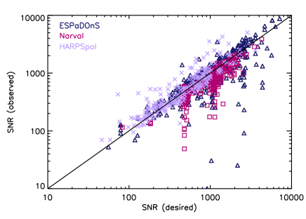
Figure 10: Left - Cumulative histograms of the predicted dipole magnetic field strength sensitivity, according to the SNRs achieved during LP observations. Right - Achieved SNRs versus those predicted according to exposure time for all SC LP observations, according to instrument (triangles for ESPaDOnS, squares for Narval and crossed for HARPSpol).

The accuracy of these empirical relations will be evaluated in forthcoming papers.

The total exposure time (in seconds) required was then computed by first dividing the required LSD SNR by the inferred LSD gain factor $G({\rm ST})$ to obtain the required SNR in the reduced spectrum, SNR_spec. Finally, we applied the appropriate official exposure time relation ETC$(V,{\rm SNR_{spec}})$ for each instrument to infer the exposure time.

In many cases, the required aggregate spectrum SNR was too high to be achieved in a single observation without saturation. In these cases, the observation was subdivided into several subsequences. The total time required to obtain an observation of many hot, bright and/or broad-lined stars was therefore often dominated by overheads.

For example, for HD 87901 (Regulus, B8IVn, $V=1.4$, $v\sin i\simeq 300$ km/s) the SNR_LSD required for a magnetic sensitivity of 250 G (i.e. $B_{\rm 0.1}=2.5$) was about 70,000. For a gain factor consistent with its spectral type ($G({\rm B8V})=14$), the required SNR_spec in the aggregate spectrum was computed to be about 5,000. Observations were acquired with ESPaDOnS. The ESPaDOnS ETC predicted a maximum exposure time (before saturation) per polarimetric subexposure of 10 s. Sixteen observations corresponding to 4 subexposures of 10 s each were acquired. The total exposure time was 640 s, whereas the total observing time including official overheads was 3200 s. Hence the overheads corresponded to 80% of the total observing time required.

For the actual observations of HD 87901, the combined SNR in the coadded Stokes $V$ spectrum was 5700, leading to an expected magnetic sensitivity (based on Eq. 2 and the observed SNR) of about 220 G.

In addition to the LP observations, a significant fraction of the SC observations were collected from the archives. Hence the exposure times and sensitivities of these observations are diverse, and adopted by the original PIs according to their scientific goals.

3.6 Quantitative magnetic diagnosis

The quantitative determination of the detection of a magnetic signature (e.g. Fig. 1) in the LSD profile is obtained in two ways. First, we use the Stokes $V$ spectra to measure the mean longitudinal magnetic field strength $\langle B_{z}\rangle$ of each star at the time of observation. We can also examine spectral lines for the presence of circular polarisation signatures: Zeeman splitting combined with Doppler broadening of lines by rotation leads to non-zero values of $V$ within spectral lines even when the value of $\langle B_{z}\rangle$ is equal to zero. This possibility substantially increases the sensitivity of our measurements as a discriminant of whether a star is in fact a magnetic star or not, as discussed by Shorlin et al. (2002); Silvester et al. (2009) and Shultz et al. (2012).

The field $\langle B_{z}\rangle$ is obtained by integrating the $I/I_{\rm c}$ and $V/I_{\rm c}$ profiles (normalized to the continuum $I_{\rm c}$) about their centres-of-gravity $v_{\rm 0}$ in velocity $v$, in the manner implemented by Rees & Semel (1979); Donati et al. (1997) and corrected by Wade et al. (2000):

$$\langle B_{z}\rangle=-2.14\times 10^{11}\ \frac{{\displaystyle\int(v-v_{\rm 0})V(v)\ dv}}{\displaystyle{\lambda zc\ \int[1-I(v)]\ dv}}.$$ (3)

In Eq. (3), $V(v)$ and $I(v)$ are the $V/I_{\rm c}$ and $I/I_{\rm c}$ profiles, respectively. The wavelength $\lambda$ is expressed in nm and the longitudinal field $\langle B_{z}\rangle$ is in gauss. The wavelength and Landé factor $z$ correspond to those used to normalize the LSD profile at the time of extraction. Atomic data were obtained from the Vienna Atomic Line Database (VALD) where available. When experimental Landé factors were unavailable, they were calculated assuming L-S coupling. The limits of integration are usually chosen for each star to coincide with the observed limits of the LSD $I$ and $V$ profiles ; using a smaller window would neglect some of the signal coming from the limb of the star, while a window larger than the actual line would increase the noise without adding any further signal, thus degrading the SNR below the optimum value achievable (see e.g. Neiner et al., 2012c).

In addition, the LSD Stokes $V$ profile is itself examined. We evaluate the false alarm probability (FAP) of $V/I_{\rm c}$ inside the line according to:

$${\rm FAP}(\chi^{2}_{r},\nu)=1-P({\nu\over{2}},{{\nu\chi^{2}_{r}}\over{2}}),$$ (4)

where $P$ is the incomplete gamma function, $\nu$ is the number of spectral points inside the line, and $\chi^{2}_{r}$ is the reduced chi-square ($\chi^{2}/\nu$) computed across the $V$ profile (e.g. Donati, Semel & Rees, 1992). The reference level required to compute $\chi^{2}/\nu$, while in principle equal to $V=0$, may be affected by small offsets related to instrumentation and data reduction. In this work, to avoid potential systematics related to such offsets, we employ the mean of $V$, measured outside of the spectral line, as the reference for calculation of $\chi^{2}/\nu$. The FAP value gives the probability that the observed $V$ signal inside the spectral line could be produced by chance if there is actually no field present. Thus a very small value of the FAP implies that a field is actually present. We evaluate FAP using the detection thresholds of Donati et al. (1997). We consider that an observation displays a “definite detection” (DD) of Stokes $V$ Zeeman signature if the FAP is lower than 0.00001, a “marginal detection” (MD) if it falls between 0.001 and 0.00001, and a “null detection” (ND) otherwise. As mentioned above a significant signal (i.e. with a MD or DD) may occur even if $\langle B_{z}\rangle$ is not significantly different from zero. Normally, a star was considered to have been detected if a significant signal (i.e. with a MD or DD) was detected within the line, while always remaining insignificant in the neighbouring continuum and in the $N$ profile.

4 Polarimetric performance and quality control

4.1 Overview of data quality

Data quality was quantified and monitored in several ways during acquisition and analysis.

We adopt SNR per spectral pixel in the reduced, 1-dimensional polarimetric spectra as our principal indicator of data quality. For ESPaDOnS and Narval spectra, this corresponds to a 1.8 km/s pixel measured in the null spectrum, whereas for HARPSpol spectra, the spectral bin is 0.8 km/s. SNR is defined as the inverse of the formal uncertainty of each pixel normalized to the continuum, and is determined from counting statistics by tracking photons through the entire spectral reduction process. As a consequence, each reduced spectrum is accompanied by error bars (i.e. 1/SNR) associated with each pixel. The accuracy of the SNR calculation is verified using measurements of the RMS deviation in the diagnostic null.

The distribution of SNRs of the TC and SC spectra is illustrated in Fig. 11. The distribution is very broad, extending from values of a few tens, and with a tail extending to $>2000$. The median SNR is 800. The breadth and structure of the distribution can be ascribed to three factors. First, recall that the desired SNR of each SC target was computed in order to achieve a particular magnetic sensitivity, and that such a calculation is a function of the stellar spectral characteristics (spectral type, $v\sin i$; see Fig. 8). Hence stars with different spectral characteristics can require significantly different SNRs to achieve the same magnetic sensitivity. Moreover, as described in §3.5, a range of magnetic sensitivity targets was adopted in this study. Secondly, recall that TC targets were observed repeatedly, and that the observations of a particular TC target typically have roughly the same SNR. Finally, archival data included in the SC have diverse SNR characteristics that were presumably determined by the scientific requirements of the associated programs. The form and structure of the SNR distribution are mainly a consequence of these effects, in addition to poor weather.

Figure 11: Distributions of SNRs per spectral pixel at 500 nm. For comparison, the spectrum shown in Fig. 1 has a SNR of 860. Different colours and linestyles are used to distinguish between all, LP, and archival (PI) observations.

Fig. 10 (left panel) shows the cumulative histograms of the predicted surface dipole field strength sensitivities, based on the SNRs achieved during the LPs. For the combined sample, 50% of observations are estimated to be sensitive to surface dipole magnetic fields equal to or stronger than 375 G. Note that, in particular, for 75% of the observed sample we predict sensitivity to dipole fields of 1 kG or weaker. These predicted sensitivities will be evaluated in greater detail in future papers. The right panel summarizes the achieved SNRs per spectral pixel as compared to the desired SNRs computed using the exposure time model, for the LP SC observations. The results are in reasonable agreement with the 1:1 relationship, indicating that the dataset fulfils the initial requirements.

As is discussed by Silvester et al. (2012), the ESPaDOnS and Narval instruments exhibit small differences in resolving power (2-3%) relative to each other, and small variations of resolving power with time. Such small differences and variations should have no significant impact on the quality of the magnetic measurements. Our data are consistent with these conclusions. Silvester et al. (2012) also demonstrate the good agreement between magnetic analyses performed using ESPaDOnS and Narval.

The HARPSpol instrument differs from ESPaDOnS and Narval in terms of its general design and optical strategy, ultimately leading to polarized spectra covering a smaller wavelength window but with significantly higher resolution. Due to the locations of the instruments in different hemispheres, there are as yet few examples of magnetic stars that have been monitored by both HARPSpol and the northern instruments in order to verify their spectral and polarimetric agreement in detail. However, Piskunov et al. (2011) (in their figure 5) illustrate the agreement of the Stokes $I$ and $V$ spectra of the sharp-lined Ap star $\gamma$ Equ, and Bailey, Grunhut & Landstreet (2015) demonstrate (in their figure 1) that the longitudinal field of HD 94660 as measured by ESPaDOnS agrees with the variation inferred form HARPSpol measurements.

4.2 TC targets as magnetic and spectral standards

The principal method of monitoring the accuracy and precision of the polarimetric analysis of all 3 instruments was through the examination of the recurrent observations of magnetic stars (typically TC targets).

Repeated observations of many TC targets confirm their strict periodicity on the timescale of the MiMeS observations (e.g. Wade et al., 2011; Grunhut et al., 2012b; Yakunin et al., 2015). This periodic variability, on timescales ranging from less than 1 day to more than 1 year, provides a powerful method to verify the long-term stability of the polarimetric performance of the instruments, as well as the compatibility of their magnetic analyses. Figures 12 and 13 illustrate the longitudinal magnetic field variations, from both the Stokes $V$ and diagnostic $N$ profiles (shown at the same display scale as $V$), for two MiMeS TC targets: HD 184927, a strong-field early Bp star studied by Yakunin et al. (2015), and V2052 Oph, a weak-field $\beta$ Cep star studied by Neiner et al. (2012a).

For HD 184927, 28 good-quality Stokes $V$ measurements were obtained with ESPaDOnS between HJD 2454667 (July 20 2008) and 2456105 (June 27 2012), corresponding to 1438 days or approximately 4 years of observation. The rotational period of HD 184927 is 9.53 days, and the time over which the data were acquired corresponds to more than 150 stellar rotations. The median error bar of the longitudinal field measurements from LSD profiles is 15 G, and the reduced $\chi^{2}$ of a sinusoidal fit with fixed period is 0.6. Clearly all of the measurements of HD 184927 agree very well with a sinusoidal variation stable within $\sim 15$ G during the period 2008-2012.

(a)

(b)

(c)

Figure 12: Longitudinal field measurements of the strong-field ESPaDOnS TC target HD 184927 ($P_{\rm rot}=9.53$ d). Adapted from Yakunin et al. (2015).

(a)

(b)

(c)

Figure 13: Longitudinal field measurements of the weak-field Narval TC target V2052 Oph ($P_{\rm rot}=3.64$ d). Adapted from Neiner et al. (2012a).

For V2052 Oph, 44 good-quality Stokes $V$ measurements were obtained with Narval between HJD 2454286 (July 4 2007) and HJD 2455421 (August 12 2010), corresponding to 1135 days or approximately 3.1 years of observation. The rotational period of V2052 Oph is 3.64 days, and the time over which the data were acquired corresponds to more than 300 stellar rotations. The median error bar of the longitudinal field measurements from LSD profiles is 21 G. A purely sinusoidal fit provides a good reproduction of the phase variation of the observations, resulting in a reduced $\chi^{2}$ of 1.2. These results are consistent with those reported by Neiner et al. (2012a), and demonstrate the long-term repeatability of measurements of even a relatively weak magnetic field. All of the measurements of V2052 Oph agree well with this unique harmonic variation stable within $\sim 20$ G during the period 2007-2010.

The long-term agreement of these measurements provides confidence that no unidentified instrumental changes (e.g. associated with instrument mounting/dismounting, change of the ESPaDOnS CCD, short-term and long-term drifts, etc.) have occurred during the MiMeS project. It also demonstrates that the measurements are insensitive to the ESPaDOnS instrumental crosstalk, which was systematically reduced from $\sim 5$% to below 1% during the course of the project.

In the context of the recent examinations of magnetometry obtained with the low-resolution FORS spectropolarimeters (Bagnulo et al., 2012; Landstreet, Bagnulo & Fossati, 2014), Figs. 12 and 13 are of great interest. In contrast to FORS1, there does not, except for the short period of malfunction of the Narval rhomb #2, discussed in §2.4), seem to be any problem of occasional statistically significant outliers. As a result, small data sets can be safely used to estimate periods, for example, without fear that the period obtained is badly polluted by one 4-5$\sigma$ outlier.

Secondly, another problem identified clearly with FORS data is the need to ensure that all measurements are on the same instrumental system. This is especially important when constructing magnetic curves and using them to determine new or improved periods. It has been established for FORS1 (Landstreet, Bagnulo & Fossati, 2014) that each choice of grism and wavelength window constitutes a distinct instrumental measuring system, and that simultaneous field measurements in different instrumental systems may result in significantly different field strengths. Fig. 14 shows spectra and LSD profiles of the magnetic TC target HD 37776 acquired using two different instruments (ESPaDOnS and Narval), at the same rotational phase on dates separated by about 21 days. The Stokes $I$ and $V$ profiles are identical to within the uncertainties. The right panel shows phased longitudinal field measurements obtained with both ESPaDOnS and Narval for the same star, demonstrating that the two instrumental systems are essentially identical and data from the two instruments may be confidently combined. This includes $\langle B_{z}\rangle$ measurements and LSD profiles (e.g. Fig. 14), as long as they are extracted using the same line mask applied to the same spectral regions (which was the case for all MiMeS observations).

Figure 14: Comparison of ESPaDOnS and Narval observations of HD 37776 (rotational period $P_{\rm rot}=1.54$ d). Left - Comparison of ESPaDOnS (black) and Narval (red) Stokes $I$ and $V$ spectra of the TC target HD 37776 at phase 0.34, obtained 21 days apart. A small part of the red region of the spectrum showing the H$\alpha$ line. Middle - Comparison of LSD profiles extracted from the full ESPaDOnS and Narval spectra at the same phase. Right - Comparison of all longitudinal field measurements of HD 37776 obtained with ESPaDOnS and Narval, phased according to the ephemeris of Mikulášek et al. (2008). The solid curve is a 3rd-order harmonic fit to the combined data. Observations were obtained between JDs 2454845 and 2455967, i.e. over a period of more than 3 years. The internal and external agreement of the datasets is excellent. Adapted from Shultz et al., in prep.

Examples of MiMeS observations of TC targets acquired with the HARPSpol instrument are reported by Alecian et al. (2011, 2014). These observations span a shorter time than those described above. Other monitoring observations (such as those of Rusomarov et al., 2013) better demonstrate the long-term stability of the HARPSpol instrument.

These examples, published and proprietary observations of other MiMeS TC targets (see Table 4), and complementary published results (e.g. Silvester et al., 2012) provide a strong verification of the long term stability of the sensitivity, zero point, and scale of magnetic measurements acquired with ESPaDOnS and Narval. HARPSpol was commissioned only in 2011, so more limited data exist with which to evaluate its long-term stability and compatibility of its measurements with those obtained with other spectropolarimeters. However, the existing data suggest very good agreement and stability.

5 Summary and conclusions

The MiMeS survey of Magnetism in Massive Stars is by far the largest systematic survey of massive star magnetism ever undertaken. The goal of this project is to unravel the origin of magnetic fields in massive stars, and to understand the impact of magnetic fields on stellar mass loss and environment, rotational evolution, and ultimately stellar evolution.

This paper has described the methodology of the project. Many papers reporting analyses of TC targets have already been published in conference proceedings and refereed journals (e.g. Oksala et al., 2010; Wade et al., 2011; Neiner et al., 2012a; Bailey et al., 2012; Kochukhov et al., 2014; Yakunin et al., 2015). In addition, many of the magnetic stars that were newly-detected or confirmed during the SC have been followed up and are discussed in refereed papers. For the O stars, these include Grunhut et al. (2009, 2012b, 2013); Martins et al. (2010); Wade et al. (2012a, b, 2015) and Sundqvist et al. (2013). For B stars, these include Petit et al. (2011); Alecian et al. (2011); Grunhut et al. (2012a); Briquet et al. (2013); Neiner, Tkachenko & MiMeS Collaboration (2014); Alecian et al. (2014), and Shultz et al. (2015).

Similarly, some TC and SC null results of particular significance have already been published. These include measurements of Wolf-Rayet stars (de la Chevrotière et al., 2013, 2014), bright O and B stars exhibiting DACs (David-Uraz et al., 2014), BA supergiants (Shultz et al., 2014), and a number of B stars in which detections of magnetic fields were previously claimed but that were not confirmed by independent MiMeS observations (Shultz et al., 2012).

The present paper has concentrated on the SC. The survey comprises over 4800 circularly polarized spectra of 106 O and WR stars, and 422 B stars, ranging from spectral type O4 to B9.5 $V\sim 0$ to 13.6. We have acquired data of these 528 stars thanks to large programs of observations with the three high resolution spectropolarimeters available in the world: ESPaDOnS@CFHT, Narval@TBL, and HARPSpol@ESO. We have established the reliability of the observational tools by comparing the data obtained from the three instruments, as well as the obtained versus initially expected quality of the data. We have shown that the data are mutually consistent and perfectly suitable for our science goals.

In particular, these high resolution, high SNR spectropolarimetric data allow us to determine the fundamental parameters of each target (see Martins et al., 2015, for the O stars), as well as the magnetic field and magnetospheric properties (e.g. Petit et al., 2013). While this paper introduces the MiMeS survey, a series of forthcoming papers will present the magnetic analysis of several subsamples of stars: the O, B, classical Be, pulsating OB, OB supergiants, and cluster stars. Interpretation of the null results for all O and B stars in terms of upper field limits will also be published, as well as the fundamental parameters of the B stars (for the O stars, see Martins et al., 2015). Ultimately, the survey results will allow us to quantify the occurence of magnetic fields in massive stars and search for correlation between the properties of magnetic fields and stellar properties.

This article represents the introduction to the MiMeS survey. Nine additional papers related to the SC are currently planned or in preparation:

• Magnetic analysis of the O-stars sample (Grunhut et al., in prep)

• Interpretation of the O-stars null results (Petit et al., in prep)

• Magnetic analysis of the classical Be stars sample (Neiner et al., in prep)

• Magnetic analysis of the O and B supergiants sample (Oksala et al., in prep)

• Magnetic analysis of the open clusters sample (Alecian et al., in prep)

• Magnetic analysis of the pulsating OB stars (Neiner et al., in prep)

• Magnetic analysis of the B-stars sample (Grunhut et al., in prep)

• Interpretation of the B-stars null results (Petit et al., in prep)

• Physical parameters of the B-stars sample (Landstreet et al., in prep)

Table 5: MiMeS O-type and WR SC targets. Columns report common identifier and HD #, $V$ band magnitude, the number of ESPaDOnS (E), Narval (N) and HARPSpol (H) spectra acquired, and the total number of spectra, the spectral type, luminosity class (LC) and any spectral peculiarity (pec), and the reference to the spectral type, luminosity class and peculiarity.

			# of observations
Name	HD	V	E	N	H	Tot	Spectral type	LC	pec	Reference
HD 108	108	7.38	23	87	0	110	O8		f?p var	Sota et al. (2011)
AO Cas	1337	6.1	1	0	0	1	O9.5	II	(n)	Sota et al. (2011)
WR 1	4004	10.14	4	0	0	4	WN4b			Crowther (2014)
V354 Per	13745	7.9	0	3	0	3	O9.7	II	(n)	Sota et al. (2011)
HD 14633	14633	7.47	1	0	0	1	ON8.5	V		Sota et al. (2011)
HD 17505	17505	7.1	1	0	0	1	O6.5	III	n((f))	Sota et al. (2011)
HD 24431	24431	6.8	2	0	0	2	O9	III		Sota et al. (2011)
X Per	24534	6.72	2	0	0	2	O9.5:		npe	Sota et al. (2011)
$\xi$ Per	24912	4.06	5	39	0	44	O7.5	III	(n)((f))	Sota et al. (2011)
$\alpha$ Cam	30614	4.3	10	1	0	11	O9	Ia		Sota et al. (2011)
AE Aur	34078	6	1	11	0	12	O9.5	V		Sota et al. (2011)
HD 34656	34656	6.8	1	0	0	1	O7.5	II	(f)	Sota et al. (2011)
HD 35619	35619	8.66	1	0	0	1	O7.5	V	((f))	Sota et al. (2011)
LY Aur	35921	6.85	1	0	0	1	O9.5	II		Sota et al. (2011)
$\delta$ Ori A	36486	2.41	0	11	0	11	O9.5	II	Nwk	Sota et al. (2011)
$\upsilon$ Ori	36512	4.62	0	1	0	1	O9.7	V		Sota et al. (2011)
$\lambda$ Ori A	36861	3.3	9	11	0	20	O8	III	((f))	Sota et al. (2011)
HD 36879	36879	7.58	3	0	0	3	O7	V	(n)((f))	Sota et al. (2011)
43 Ori	37041	5.08	11	0	0	11	O9.5	IV	p	Sota et al. (2011)
$\iota$ Ori	37043	2.77	12	0	0	12	O9	III	var	Sota et al. (2011)
HD 37366	37366	7.64	1	0	0	1	O9.5	IV		Sota et al. (2011)
$\sigma$ Ori	37468	3.8	5	0	0	5	O9.7	III		Sota et al. (2011)
$\mu$ Col	38666	5.15	2	0	0	2	O9.5	V		Sota et al. (2013)
HD 42088	42088	7.56	1	0	0	1	O6	V	((f))z	Sota et al. (2011)
HD 46056	46056	8.16	2	0	0	2	O8	V	n	Sota et al. (2011)
HD 46106	46106	7.948	1	0	0	1	O9.7	II-III		Sota et al. (2011)
HD 46149	46149	7.59	6	0	0	6	O8.5	V		Sota et al. (2011)
HD 46150	46150	6.75	8	0	0	8	O5	V	((f))z	Sota et al. (2011)
HD 46202	46202	8.2	3	0	0	3	O9.5	V		Sota et al. (2011)
HD 46223	46223	7.32	5	0	0	5	O4	V	((f))	Sota et al. (2011)
HD 46485	46485	8.2	5	0	0	5	O7	V	n	Sota et al. (2011)
HD 46966	46966	6.87	1	0	0	1	O8.5	IV		Sota et al. (2011)
V640 Mon	47129	6.06	38	4	0	42	O8		fp var	Sota et al. (2011)
V689 Mon	47432	6.24	1	0	0	1	O9.7	Ib		Sota et al. (2011)
15 Mon	47839	4.64	3	13	0	16	O7	V	((f)) var	Sota et al. (2011)
HD 48099	48099	6.37	2	1	0	3	O6.5	V	(n)((f))	Sota et al. (2011)
HD 54662	54662	6.23	2	0	0	2	O7	V	((f))z var?	Sota et al. (2011)
HD 55879	55879	6.0	1	0	0	1	O9.7	III		Sota et al. (2011)
HD 57682	57682	6.4	37	0	0	37	O9.5	IV		Sota et al. (2011)
HD 66788	66788	9.43	2	0	0	2	O8	V		Robert et al. (2003)
$\zeta$ Pup	66811	2.25	30	0	5	35	O4	I	f	Sota et al. (2013)
WR 11	68273	1.83	12	0	0	12	WC8+O7.5III-V			Crowther (2014)
HD 69106	69106	7.13	1	0	0	1	O9.7	In		Sota et al. (2013)
HD 93028	93028	8.36	0	0	2	2	O9	IV		Sota et al. (2011)
HD 93250	93250	7.5	0	0	2	2	O4	III	fc:	Sota et al. (2011)
HD 148937	148937	6.77	32	0	0	32	O6		f?p	Sota et al. (2013)
$\mu$ Nor	149038	4.914	3	0	0	3	O9.7	Iab		Sota et al. (2011)
$\zeta$ Oph	149757	2.58	20	46	0	66	O9.5	IV	nn	Sota et al. (2011)
V973 Sco	151804	5.249	0	0	2	2	O8	Ia		Sota et al. (2011)
HD 152233	152233	6.59	1	0	0	1	O6	Ib	(f)	Sota et al. (2013)
HD 152247	152247	7.2	1	0	0	1	O9.5	III		Sota et al. (2013)
HD 152249	152249	6.47	1	0	0	1	OC9	Iab		Sota et al. (2011)
HD 152408	152408	5.77	3	0	0	1	O9	II-III		Sota et al. (2013)
HD 153426	153426	7.49	2	0	0	2	O9	II-III		Sota et al. (2013)
V884 Sco	153919	6.53	1	0	0	1	O6	Ia	f	Sota et al. (2013)
V1074 Sco	154368	6.18	1	0	0	1	O9.5	Iab		Sota et al. (2011)
HD 154643	154643	7.15	1	0	0	1	O9.5	III		Sota et al. (2011)

Table 6: continued

MiMeS O-type and WR SC targets.

			# of observations
Name	HD	V	E	N	H	Tot	Spectral type	LC	pec	Reference
HD 155806	155806	5.612	25	0	0	25	O7.5	V		Sota et al. (2013)
HD 155889	155889	6.565	0	0	1	1	O9.5	IV		Sota et al. (2011)
HD 156154	156154	8.04	1	0	0	1	O7.5	Ib		Sota et al. (2011)
63 Oph	162978	6.2	5	0	0	5	O8	II	((f))	Sota et al. (2011)
HD 164492	164492	7.53	1	0	0	1	O7.5	V	z	Sota et al. (2013)
9 Sgr	164794	5.93	14	3	0	17	O4	V	((fc))	Sota et al. (2013)
HD 165052	165052	6.84	1	0	0	1	O5.5:+O8:	Vz+V		Sota et al. (2011)
WR 111	165763	7.82	16	0	0	16	WC5			Crowther (2014)
16 Sgr	167263	5.97	1	0	0	1	O9.5	II-III	n	Sota et al. (2013)
15 Sgr	167264	5.347	5	7	0	12	O9.7	Iab		Sota et al. (2013)
HD 167771	167771	6.54	2	0	0	2	O7	III	(f)	Sota et al. (2011)
HD 186980	186980	7.48	1	0	0	1	O7.5	III	((f))	Sota et al. (2013)
9 Sge	188001	6.24	1	0	0	1	O7.5	Iab	f	Sota et al. (2011)
HD 188209	188209	5.63	1	27	0	28	O9.5	Iab		Sota et al. (2011)
HD 189957	189957	7.82	1	0	0	1	O9.7	III		Sota et al. (2013)
WR 133	190918	6.75	3	0	0	3	WN5o+O9I			Crowther (2014)
HD 191201	191201	7.34	1	0	0	1	O9.5+B0	III+IV	((n))	Sota et al. (2011)
WR 134	191765	8.08	38	0	0	38	WN6b			Crowther (2014)
WR 135	192103	8.11	13	0	0	13	WC8			Crowther (2014)
WR 136	192163	7.5	9	0	0	9	WN6b		(h)	Crowther (2014)
V2011 Cyg	192281	7.55	0	2	0	2	O4.5	V	n(f)	Sota et al. (2011)
HD 192639	192639	7.11	0	1	0	1	O7.5	Iab	f	Sota et al. (2011)
WR 137	192641	7.91	27	0	0	27	WC7pd+O9			Crowther (2014)
WR 138	193077	8.01	6	0	0	6	WN6o			Crowther (2014)
HD 193322	193322	5.82	2	0	0	2	O9	IV	(n)	Sota et al. (2011)
HD 193443	193443	7.24	1	0	0	1	O9	III		Sota et al. (2011)
WR 139	193576	8.00	9	0	0	9	WN5o+O6III-V			Crowther (2014)
WR 140	193793	6.85	19	0	0	19	WC7pd+O4-5			Crowther (2014)
HD 199579	199579	5.97	4	0	0	4	O6.5	V	((f))z	Sota et al. (2011)
HD 201345	201345	7.75	1	0	0	1	ON9.5	IV		Sota et al. (2011)
68 Cyg	203064	5.04	5	3	0	8	O7.5	III	n((f))	Sota et al. (2011)
HD 204827	204827	8.00	1	0	0	1	O9.7	III		Sota et al. (2011)
HD 206183	206183	7.41	1	0	0	1	O9.5	IV-V		Sota et al. (2011)
HD 206267	206267	5.62	6	0	0	6	O6.5	V	((f))	Sota et al. (2011)
HD 207198	207198	5.96	1	15	0	16	O9	II		Sota et al. (2011)
HD 207538	207538	7.3	1	0	0	1	O9.7	IV		Sota et al. (2011)
14 Cep	209481	5.55	3	11	0	14	O9	IV	(n) var	Sota et al. (2011)
19 Cep	209975	5.11	7	26	0	33	O9	Ib		Sota et al. (2011)
HD 210809	210809	7.56	1	0	0	1	O9	Iab		Sota et al. (2011)
$\lambda$ Cep	210839	5.08	0	26	0	26	O6.5	I	(n)fp	Sota et al. (2011)
10 Lac	214680	4.88	1	35	0	36	O9	V		Sota et al. (2011)
HD 218195	218195	8.44	1	0	0	1	O8.5	III		Sota et al. (2011)
HD 218915	218915	7.2	1	0	0	1	O9.5	Iab		Sota et al. (2011)
HD 227757	227757	9.27	2	0	0	2	O9.5	V		Maiz Apellaniz (priv. comm.)
HD 258691	258691	9.7	3	0	0	3	O9.5	IV		Maiz Apellaniz (priv. comm.)
HD 328856	328856	8.5	1	0	0	1	O9.7	Ib		Sota et al. (2013)
BD+60 499		10.27	1	0	0	1	O9.5	V		Sota et al. (2011)
CD-28 5104		10.09	44	0	2	46	O6.5		f?p	Sota et al. (2013)
BD-13 4930		9.37	1	0	0	1	O9.7	V		Maiz Apellaniz (priv. comm.)
NGC 1624 2		11.77	17	1	0	18	O7		f?p	Sota et al. (2011)

Table 7: MiMeS B-type SC targets. Columns report common identifier and HD #, $V$ band magnitude, the number of ESPaDOnS (E), Narval (N) and HARPSpol (H) spectra acquired, and the total number of spectra, the spectral type, luminosity class (LC) and any spectral peculiarity (pec), and the reference to the spectral type, luminosity class and peculiarity. ’BSC’ indicates the Bright Star Catalogue (Hoffleit & Jaschek, 1991).

			# of observations
Name	HD	V	E	N	H	Tot	Spectral type	LC	pec	Reference
$\alpha$ And	358	2.058	16	0	0	16	B8	IV	p MnHg	BSC
$\gamma$ Peg	886	2.83	6	23	0	29	B2	IV		BSC
HD 955	955	7.369	0	0	2	2	B4	V		Reed (2003)
V746 Cas	1976	5.575	0	16	0	16	B5	IV		BSC
$\kappa$ Cas	2905	4.189	3	0	0	3	B1	Ia	e	BSC
53 Psc	3379	5.864	1	10	0	11	B2.5	IV		BSC
$\gamma$ Cas	5394	2.47	0	58	0	58	B0	IV	e	BSC
V442 And	6226	6.82	1	0	0	1	B2	IV/V		Guetter (1968)
V764 Cas	7636	6.891	6	0	0	6	B2	III	:[n]e+	Walborn (1971)
$\alpha$ Eri	10144	0.5	0	0	18	18	B3	V	pe	BSC
$\phi$ Per	10516	4.09	6	0	0	6	B2	V	ep	BSC
HD 10747	10747	8.15	0	0	2	2	B2	V		Houk & Cowley (1975)
$\epsilon$ Cas	11415	3.342	1	1	0	2	B3	III		BSC
CG Hyi	11462	7.8	0	0	20	20	B8	V		Houk & Cowley (1975)
V520 Per	14134	6.543	2	0	0	2	B3	Ia		Morgan, Code & Whitford (1955)
$\delta$ Cet	16582	4.07	0	5	0	5	B2	IV		BSC
89 Cet	17081	4.235	2	4	0	6	B7	V		BSC
$\theta$ Hyi	19400	5.497	0	0	4	4	B3+A0	V+IV		BSC
HD 20001	20001	7.03	0	0	1	1	B3	V		Houk & Smith-Moore (1988)
BK Cam	20336	4.728	5	1	0	6	B2.5	V	en	BSC
V576 Per	21071	6.071	0	3	0	3	B7	V		BSC
$\psi$ Per	22192	4.31	0	7	0	7	B5	V	e	BSC
17 Tau	23302	3.705	0	2	0	2	B6	III	e	BSC
$\eta$ Tau	23630	2.873	0	1	0	1	B7	III	e	BSC
$\zeta$ Per	24398	2.883	2	0	0	2	B1	Ib		BSC
33 Eri	24587	4.625	4	2	0	6	B6	V		BSC
HD 24640	24640	5.489	0	1	0	1	B1.5	V		BSC
$\epsilon$ Per	24760	2.901	0	3	0	3	B0.5+A2	V+V		BSC
$\lambda$ Tau	25204	3.408	1	0	0	1	B3+A4	V+IV		BSC
40 Tau	25558	5.308	12	19	0	31	B3	V		BSC
GU Eri	26326	5.427	1	6	0	7	B4	V		BSC
49 Tau	26912	4.28	3	0	0	3	B3	IV		BSC
53 Per	27396	4.814	0	3	0	3	B4	IV		BSC
V1141 Tau	27742	5.996	0	3	0	3	B8	IV-V		BSC
V1143 Tau	28114	6.067	2	0	0	2	B6	IV		BSC
V1144 Tau	28475	6.775	1	0	0	1	B5	V		BSC
$\delta$ Cae	28873	5.053	0	0	1	1	B2	IV-V		BSC
$\nu$ Eri	29248	3.92	2	2	0	4	B2	III		BSC
3 Ori	30836	3.68	1	0	0	1	B2+B2	III+IV		BSC
AB Aur	31293	7.06	2	0	0	2	A1		HAeBe	Hernández et al. (2004)
11 Cam	32343	5.03	8	0	0	8	B2.5	V	e	BSC
HZ Aur	32633	7.07	6	0	0	6	B9		p SiCr	Renson & Manfroid (2009)
105 Tau	32991	5.92	2	1	0	3	B2	V	e	BSC
$\lambda$ Eri	33328	4.249	5	0	0	5	B2	IV	ne	BSC
$\beta$ Ori	34085	0.12	0	34	0	34	B8	Ia	e:	BSC
$\rho$ Aur	34759	5.2	4	0	0	4	B3	V		BSC
YZ Lep	34798	6.39	1	1	0	2	B3	V		BSC
V1156 Ori	35298	7.91	0	2	0	2	B6		p Hewk	Renson & Manfroid (2009)
$\eta$ Ori	35411	3.38	6	2	0	8	B1+B2	V+?	e	BSC
$\gamma$ Ori	35468	1.64	9	0	0	9	B2	III		BSC
114 Tau	35708	4.865	2	0	0	2	B2.5	IV		BSC
$\psi$ Ori	35715	4.595	6	0	0	6	B2	IV		BSC
HD 35912	35912	6.382	11	0	0	11	B2	V		BSC

Table 8: continued

MiMeS B-type SC targets.

			# of observations
Name	HD	V	E	N	H	Tot	Spectral type	LC	pec	Reference
HD 36629	36629	7.64	1	0	1	B2.5	IV			Abt & Levato (1977)
37 Ori	36822	4.398	1	0	0	1	B0	III		BSC
HD 36959	36959	5.67	1	0	0	1	B1	V	v	BSC
HD 36960	36960	4.78	1	0	0	1	B0.5	V		BSC
V1046 Ori	37017	6.553	10	0	0	10	B1.5	V		BSC
41 Ori A	37020	6.73	3	0	0	3	B0.2	V		Maiz Apellaniz (priv. comm.)
41 Ori D	37023	6.71	4	0	0	4	B0.5	V	p	BSC
HD 37042	37042	6.02	1	0	0	1	B0.5	V		Nieva (2013)
$\epsilon$ Ori A	37128	1.7	9	61	0	70	B0	Ia	e	BSC
$\zeta$ Tau	37202	3.03	0	3	0	3	B4	III	pe	BSC
HD 37525Ab	37525	8.06	2	0	0	2	B5			Caballero, Albacete-Colombo & López-Santiago (2010)
$\alpha$ Col	37795	2.6	6	0	0	6	B7	IV	e	BSC
HD 38120	38120	9.08	0	1	0	1	B9		e	Vieira et al. (2003)
$\kappa$ Ori	38771	2.049	36	0	0	36	B0.5	Ia	v	BSC
$\gamma$ Col	40494	4.35	1	0	0	1	B2.5	IV		BSC
62 Ori	41117	4.646	1	0	0	1	B2	Ia	ve	BSC
HD 43317	43317	6.611	0	19	0	19	B3	IV		BSC
7 Mon	44112	5.246	0	1	0	1	B2.5	V		BSC
$\zeta$ CMa	44402	3	0	0	2	2	B2.5	V		BSC
HD 44506	44506	5.525	0	0	1	1	B1.5	V	e	BSC
$\beta$ CMa	44743	2	1	0	0	1	B1	II-III		BSC
HD 45284	45284	7.37	1	0	0	1	B6	V		Dworetsky, Whitelock & Carnochan (1982)
10 Mon	45546	5.035	0	1	0	1	B2	V		BSC
$\beta^{1}$ Mon A	45725	4.62	2	0	0	2	B3	V	e	BSC
V727 Mon	46005	8	1	0	0	1	B3	IV		Wang et al. (2008)
4 CMa	46328	4.33	25	0	0	25	B0.5	IV		BSC
HD 46769	46769	5.791	0	2	0	2	B8	Ib		BSC
V684 Mon	47755	8.43	2	0	0	2	B4	V		Wang et al. (2008)
HD 47934	47934	8.88	3	1	0	4	B7	V		Perez, The & Westerlund (1987)
HD 47961	47961	7.51	1	0	0	1	B2	V		Perez, The & Westerlund (1987)
HD 48055	48055	9	2	0	0	2	B3	V		Turner (1976)
10 CMa	48917	5.222	0	0	1	1	B2	III	e	BSC
16 Mon	48977	5.92	1	1	0	2	B2.5	V		BSC
V739 Mon	49330	8.95	0	44	0	44	B1	IV	nep	Perez, The & Westerlund (1987)
V715 Mon	49567	6.146	2	3	0	5	B3	II-III		BSC
$\kappa$ CMa	50013	3.515	0	0	3	3	B1.5	IV	ne	BSC
V742 Mon	50083	6.92	0	2	0	2	B2	:V	:nne	Morgan, Code & Whitford (1955)
HD 50209	50209	8.36	0	15	0	15	B8	IV	e	Frémat et al. (2006)
15 CMa	50707	4.806	5	0	0	5	B1	IV		BSC
HD 50820	50820	6.27	1	0	0	1	B3+K2	IV+II	e	BSC
HD 51756	51756	7.18	0	1	0	1	B	V		Wang et al. (2008)
$\epsilon$ CMa	52089	1.513	2	0	0	2	B2	II		BSC
GU CMa	52721	6.58	0	2	0	2	B3	V	ne?	Wang et al. (2008)
19 Mon	52918	4.99	0	8	0	8	B1	V		BSC
V750 Mon	53367	7.04	2	5	0	7	B0	IV	:e	Morgan, Code & Whitford (1955)
FN CMa	53974	5.39	2	4	0	6	B0.5	IV		BSC
FV CMa	54309	5.71	1	0	0	1	B2I	V	e	BSC
26 CMa	55522	5.895	1	0	0	1	B2	V		BSC
GY CMa	55857	6.096	0	0	2	2	B0.5	V		BSC
$\omega$ CMa	56139	4.028	4	0	0	4	B2	IV-V	e	BSC
OT Gem	58050	6.448	1	3	0	4	B2	V	e	BSC
HD 58260	58260	6.734	1	0	0	1	B2	V	p	Garrison, Hiltner & Schild (1977)
FW CMa	58343	5.2	2	0	0	2	B2.5	IV	e	BSC
HD 58509	58509	8.57	2	0	0	2	B0	V		Fitzgerald et al. (1979)

Table 9: continued

MiMeS B-type SC targets.

			# of observations
Name	HD	V	E	N	H	Tot	Spectral type	LC	pec	Reference
HD 58647	58647	6.85	0	0	1	1	B9	IV	e	Houk & Smith-Moore (1988)
$\beta$ CMi	58715	2.886	20	14	0	34	B8	V	e	BSC
FY CMa	58978	5.56	3	0	0	3	B0	IV	:pe	BSC
V343 Pup	60431	8.57	1	0	0	1	B4		p SiMg	Renson & Manfroid (2009)
PT Pup	61068	5.693	1	0	0	1	B2	III		BSC
HD 61555	61555	4.635	3	0	0	3	B6	V		BSC
HD 61556	61556	4.429	17	0	0	17	B5	IV	n	BSC
HD 62367	62367	7.13	1	0	0	1	B6	III		Jaschek et al. (1980)
HD 63425	63425	6.909	8	0	0	8	B0.5	V		Garrison, Hiltner & Schild (1977)
b Pup	64503	4.48	0	0	1	1	B2.5	V		BSC
J Pup	64760	4.234	13	0	0	13	B0.5	Ib		BSC
$\chi$ Car	65575	3.444	0	0	1	1	B3	IV	p	BSC
5 Cnc	65873	5.983	1	0	0	1	B9.5	V	n	BSC
V695 Mon	65875	6.51	2	2	0	4	B2.5	V	e	BSC
HD 66665	66665	7.81	5	16	0	21	B0.7	IV-V		Walborn (1971)
HD 66765	66765	6.622	0	0	10	10	B2	V		Garrison, Hiltner & Schild (1977)
HD 67041	67041	7.41	0	0	1	1	B3	III/IV		Houk (1978)
MX Vel	67341	6.163	0	0	2	2	B3	V	np	BSC
HD 67621	67621	6.316	0	0	8	8	B2.5	III		Garrison, Hiltner & Schild (1977)
V420 Pup	67698	6.53	1	0	0	1	B5	IV		Abt (1985)
HD 68092	68092	7.2	0	0	2	2	B3	V		Garrison, Hiltner & Schild (1977)
HD 68243	68243	4.2	0	0	1	1	B1	IV		BSC
IS Vel	68324	5.217	0	0	2	2	B1	IV	e	BSC
HD 68395	68395	8.1	0	0	3	3	B4	V		Houk (1978)
HD 68451	68451	7.32	0	0	4	4	B5	II		Houk (1978)
HD 68657	68657	5.805	0	0	1	1	B3	V		BSC
HD 71072	71072	6.89	0	2	0	2	B7	IV	e	Buscombe (1969)
HD 72067	72067	5.81	0	0	1	1	B2	V	en	BSC
HD 74273	74273	5.878	0	0	5	5	B1.5	V		BSC
$\eta$ Hya	74280	4.3	5	2	0	7	B3	V		BSC
HY Vel	74560	4.817	3	0	0	3	B3	IV		BSC
$\alpha$ Pyx	74575	3.675	3	0	0	3	B1.5	III		BSC
HD 75126	75126	7.08	0	0	1	1	B4	V		Levato & Malaroda (1975)
HD 75290	75290	8.09	0	0	2	2	B9	V		Levato & Malaroda (1975)
HD 75324	75324	7.12	0	0	2	2	B5	V		Levato & Malaroda (1975)
HD 75387	75387	6.42	0	0	1	1	B2	IV-V		BSC
HD 75446	75446	7.38	0	0	1	1	B6	V		Levato & Malaroda (1975)
HD 75657	75657	7.48	0	0	2	2	B6	III		Houk (1978)
HD 75724	75724	7.69	0	0	1	1	B2	IV		Garrison, Hiltner & Schild (1977)
HD 75758	75758	8.95	0	0	2	2	B3-5	V		Houk (1978)
f Vel	75821	5.094	2	0	0	2	B0	III		BSC
OU Vel	76534	8.02	2	0	0	2	B2/B3			Vieira et al. (2003)
HD 76838	76838	7.31	0	0	1	1	B2.5	V		Garrison, Hiltner & Schild (1977)
HD 76868	76868	8.04	2	0	0	2	B6		e	Slettebak, Wagner & Bertram (1997)
IU Vel	77320	6.05	0	0	1	1	B2.5	V	ne	BSC
IZ Vel	77475	5.541	0	0	1	1	B5	V		BSC
KK Vel	78616	6.786	0	0	1	1	B2	III		Garrison, Hiltner & Schild (1977)
E Car	78764	4.654	0	0	1	1	B2I	V	e	BSC
HD 79694	79694	5.839	0	0	1	1	B6	IV		BSC
HD 79791	79791	9.4	0	0	2	2	B9	V		Slawson & Reed (1988)
HD 80279	80279	9.45	0	0	2	2	B3	II/III		Houk (1978)
HD 80761	80761	7.256	0	0	2	2	B5	III		Houk (1978)
V335 Vel	85953	5.932	1	0	0	1	B2	III		BSC
EO Leo	87015	5.657	0	5	0	5	B2.5	IV		BSC
$\alpha$ Leo	87901	1.4	66	10	0	76	B7	V		BSC
23 Sex	89688	6.635	4	4	0	8	B2.5	IV		BSC
HD 89884	89884	7.131	0	2	0	2	B6	V		Hill (1970)

Table 10: continued

MiMeS B-type SC targets.

			# of observations
Name	HD	V	E	N	H	Tot	Spectral type	LC	pec	Reference
V507 Car	90966	6.429	0	0	2	2	B2/B3	III	:ne	Houk (1978)
HD 91120	91120	5.592	0	4	0	4	B9	V	ne	BSC
$\rho$ Leo	91316	3.87	2	5	0	7	B1	Ib		BSC
HD 91969	91969	6.51	0	0	1	1	B0	Iab	e	Evans et al. (2005)
V518 Car	92938	4.82	0	0	1	1	B4	V		BSC
$\theta$ Car	93030	2.78	0	0	3	3	B0	V	p	BSC
HD 93194	93194	4.786	0	0	1	1	B5	V	n	BSC
HD 93607	93607	4.85	0	0	1	1	B3	IV		BSC
HD 93714	93714	6.545	0	0	1	1	B2	IV/V	n	Abt & Morgan (1972)
HD 94097	94097	7.2	0	0	1	1	B3	V		Houk & Cowley (1975)
$\pi$ Cen	98718	3.9	0	0	4	4	B5	V	n	BSC
HD 98922	98922	6.76	1	0	1	2	B9		e	Vieira et al. (2003)
KR Mus	100546	6.7	0	0	1	1	B9	V	ne	Houk & Cowley (1975)
90 Leo	100600	5.94	4	0	0	4	B4	V		BSC
HD 101391	101391	6.334	0	4	0	4	B9		p HgMn:	BSC
HD 103079	103079	4.929	0	0	1	1	B4	V		BSC
31 Crt	104337	5.263	6	3	0	9	B1.5	V		BSC
$\theta^{2}$ Cru	104841	4.718	0	0	1	1	B2	IV		BSC
V863 Cen	105382	4.448	0	0	3	3	B6	III	e	BSC
$\delta$ Cen	105435	2.561	0	0	3	3	B2	IV	ne	BSC
$\rho$ Cen	105937	3.951	0	0	1	1	B3	V		BSC
$\delta$ Cru	106490	2.775	0	0	3	3	B2	IV		BSC
$\zeta$ Cru	106983	4.05	0	0	2	2	B2.5	V		BSC
$\alpha^{1}$ Cru	108248	1.4	0	0	4	4	B0.5	IV		BSC
G Cen	108257	4.805	0	0	2	2	B3	V	n	BSC
$\sigma$ Cen	108483	3.897	0	0	1	1	B2	V		BSC
$\gamma$ Mus	109026	3.83	0	0	9	9	B5	V		BSC
$\kappa$ Dra	109387	3.881	9	18	0	27	B6	III	pe	BSC
$\alpha$ Mus	109668	2.677	0	0	1	1	B2	IV-V		BSC
39 Cru	110335	4.94	0	0	1	1	B6	IV	e	BSC
BZ Cru	110432	5.316	0	0	2	2	B2		pe	BSC
$\beta$ Mus	110879	3.07	0	0	4	4	B2.5	V		BSC
HD 110956	110956	4.612	0	0	1	1	B3	V		BSC
$\beta$ Cru	111123	1.297	0	0	6	6	B0.5	III		BSC
$\mu^{2}$ Cru	112091	5.113	0	0	1	1	B5	V	ne	BSC
HD 112092	112092	3.988	0	0	1	1	B2	IV-V		BSC
f Cen	113703	4.694	0	0	2	2	B5	V		BSC
HD 113791	113791	4.264	0	0	12	12	B1.5	V		BSC
15 CVn	114376	6.28	0	2	0	2	B7	III		BSC
V958 Cen	114981	7.12	1	0	0	1	B5	V	e	Vieira et al. (2003)
HD 115846	115846	7.023	0	0	2	2	B3	IV		Houk & Cowley (1975)
V790 Cen	116072	6.198	0	0	2	2	B2.5	V	n	BSC
J Cen	116087	4.505	0	0	2	2	B3	V		BSC
$\alpha$ Vir	116658	1.04	0	8	0	8	B1+B2	III-IV+V		BSC
$\epsilon$ Cen	118716	2.265	0	0	8	8	B1	III		BSC
$\nu$ Cen	120307	3.39	0	0	2	2	B2I	V		BSC
$\eta$ UMa	120315	1.852	0	8	0	8	B3	V		BSC
$\mu$ Cen	120324	3.456	6	0	0	6	B2	IV-V	e	BSC
HD 120640	120640	5.75	0	0	1	1	B2	V	p	BSC
$\phi$ Cen	121743	3.806	0	0	2	2	B2I	V		BSC
HD 121790	121790	3.842	0	0	1	1	B2	IV-V		BSC
$\beta$ Cen	122451	0.6	0	0	63	63	B1	III		BSC
$\chi$ Cen	122980	4.343	0	0	1	1	B2	V		BSC
$\tau^{1}$ Lup	126341	4.546	0	0	1	1	B2	IV		BSC
$\sigma$ Lup	127381	4.416	17	0	0	17	B2	III		BSC
$\rho$ Lup	128345	4.034	0	0	2	2	B5	V		BSC

Table 11: continued

MiMeS B-type SC targets.

			# of observations
Name	HD	V	E	N	H	Tot	Spectral type	LC	pec	Reference
$\alpha$ Lup	129056	2.276	0	0	1	1	B1.5	III		BSC
V836 Cen	129929	8.05	1	0	0	1	B3	V		Hill (1970)
$o$ Lup	130807	4.313	0	0	12	12	B5	IV		BSC
$\beta$ Lup	132058	2.665	0	0	6	6	B2	III		BSC
$\kappa$ Cen	132200	3.13	0	0	2	2	B2	IV		BSC
HD 132955	132955	5.427	0	0	1	1	B3	V		BSC
$\pi$ Lup A	133242	4.59	0	0	2	2	B5	V		BSC
HD 133518	133518	6.396	0	0	3	3	B2	V	p HeStr	Garrison, Hiltner & Schild (1977)
$\lambda$ Lup	133955	4.07	0	0	2	2	B3	V		BSC
e Lup	134687	4.807	0	0	1	1	B3	IV		BSC
$\delta$ Lup	136298	3.203	0	0	6	6	B1.5I	V		BSC
$\epsilon$ Lup	136504	3.367	22	0	0	22	B2	IV-V		BSC
HD 137432	137432	5.442	0	0	1	1	B4	V	p	BSC
FK Boo	138003	7.84	0	3	0	3	B8		p Si	Grenier et al. (1999)
$\theta$ CrB	138749	4.153	0	6	0	6	B6	V	nne	BSC
IU Lib	138764	5.147	1	0	0	1	B6	IV		BSC
$\tau$ Lib	139365	3.644	0	0	1	1	B2.5	V		BSC
4 Lup	140008	4.717	0	0	1	1	B5	V		BSC
25 Ser	140873	5.39	1	8	0	9	B8	III		BSC
V1040 Sco	142184	5.4	27	0	0	27	B2.5	V	ne	BSC
$\rho$ Sco	142669	3.864	0	0	1	1	B2	IV-V		BSC
HD 142883	142883	5.841	0	0	1	1	B3	V		BSC
V913 Sco	142990	5.44	2	0	0	2	B5	IV		BSC
$\pi$ Sco	143018	2.89	0	0	1	1	B1+B2	V		BSC
$\delta$ Sco	143275	2.291	11	0	0	11	B0.3	IV		BSC
$\beta$ Sco A	144217	2.62	11	0	0	11	B1	V		BSC
$\beta$ Sco C	144218	4.89	0	0	1	1	B2	V		BSC
$\omega$ Sco	144470	3.946	0	0	1	1	B1	V		BSC
$\phi$ Her	145389	4.232	0	5	0	5	B9		p:Mn:	BSC
$\sigma$ Sco	147165	2.912	3	0	0	3	B2+O9.5	III+V		BSC
$\tau$ Her	147394	3.9	0	4	0	4	B5	IV		BSC
$\rho$ Oph D	147888	6.779	0	0	2	2	B3	V		Abt (1986)
$\rho$ Oph C	147932	7.27	0	0	4	4	B7	V		Abt (1986)
$\chi$ Oph	148184	4.42	0	4	0	4	B2	IV	:pe	BSC
HD 149277	149277	8.41	1	0	0	1	B2	IV	n	Garrison, Hiltner & Schild (1977)
HD 150898	150898	5.572	0	0	1	1	B0.5	Ia		BSC
HD 151985	151985	3.544	0	0	1	1	B2	IV		BSC
HD 152234	152234	5.43	1	0	0	1	B0.5	Ia		BSC
V1070 Sco	152635	7.66	1	0	0	1	B7	II		Houk (1982)
HD 153716	153716	5.727	0	0	1	1	B5	IV		BSC
k Sco	154090	4.861	0	0	1	1	B1	Ia	e	BSC
HD 154664	154664	8.73	0	0	2	2	B1	IV		Garrison, Hiltner & Schild (1977)
HD 155217	155217	8.66	0	0	2	2	B1.5	III	n	Garrison, Hiltner & Schild (1977)
HD 155273	155273	8.92	0	0	2	2	B3	IV		Houk (1982)
HD 155320	155320	8.37	0	0	2	2	B1	III		Garrison, Hiltner & Schild (1977)
HD 155450	155450	6.001	0	0	1	1	B	1II		BSC
HD 155506	155506	7.75	0	0	1	1	B1.5	V		Garrison, Hiltner & Schild (1977)
HD 155754	155754	7.96	0	0	1	1	B1	IV		Garrison, Hiltner & Schild (1977)
HD 155888	155888	8.68	0	0	2	2	B4	V		Houk (1982)
HD 156004	156004	7.82	0	0	2	2	B1	IV		Garrison, Hiltner & Schild (1977)
HD 156256	156256	8.28	0	0	2	2	B2	V	n	Garrison, Hiltner & Schild (1977)
HD 156321	156321	8.16	0	0	2	2	B1.5	III		Garrison, Hiltner & Schild (1977)
HD 156324	156324	8.76	0	0	3	3	B2	V		Roslund (1966)
HD 156424	156424	8.9	0	0	3	3	B2	V		Roslund (1966)
68 Her	156633	4.8	9	0	0	9	B1.5+B5	V+III	p	BSC
$\lambda$ Sco	158926	1.62	0	0	19	19	B2	IV		BSC
V994 Sco	160124	7.16	1	0	0	1	B3	IV-V		Houk (1982)

Table 12: continued

MiMeS B-type SC targets.

			# of observations
Name	HD	V	E	N	H	Tot	Spectral type	LC	pec	Reference
$\kappa$ Sco	160578	2.375	0	0	2	2	B1.5	III		BSC
$\iota$ Her	160762	3.8	0	3	0	3	B3	IV		BSC
V1092 Sco	163254	6.74	3	0	0	3	B2	V	SB2	Garrison, Hiltner & Schild (1977)
66 Oph	164284	4.784	24	32	0	56	B2	V	e	BSC
HD 164402	164402	5.749	2	0	0	2	B0	Ib		BSC
HD 164865	164865	7.74	0	0	2	2	B9	Ia		Garrison, Hiltner & Schild (1977)
HD 164906	164906	7.45	0	0	1	1	B1	IV	:pe	Morgan, Code & Whitford (1955)
HD 164933	164933	8.7	0	0	2	2	B0.5	V		Garrison, Hiltner & Schild (1977)
HD 167756	167756	6.286	1	0	0	1	B0.5	Ia		BSC
HD 168957	168957	6.983	1	0	0	1	B3	V		Guetter (1968)
HD 169142	169142	8.16	3	0	0	3	A9		HAeBe	Vieira et al. (2003)
$\alpha$ Tel	169467	3.477	1	0	8	9	B3	IV		BSC
HD 169820	169820	6.365	1	4	0	5	B9	V		BSC
QT Ser	170783	7.73	0	10	0	10	B5		HAeBe	Neubauer (1943)
$\lambda$ Pav	173948	4.207	0	0	2	2	B2	II-III	e	BSC
CX Dra	174237	5.9	1	0	0	1	B2.5	V	e	BSC
HD 174571	174571	8.89	0	2	0	2	B2.5	V	:[n]e	Walborn (1971)
$\sigma$ Sgr	175191	2.058	0	0	8	8	B2.5	V		BSC
64 Ser	175869	5.563	0	18	0	18	B9	III	ep:Hg:	BSC
HD 176386	176386	7.3	3	0	0	3	B9	V		Torres et al. (2006)
V545 Lyr	176582	6.404	0	44	0	44	B5	IV		BSC
V4024 Sgr	178175	5.57	1	0	0	1	B2	V	e	BSC
V338 Sge	179588	6.69	1	0	0	1	B9	IV		BSC
V1449 Aql	180642	8.29	11	6	0	17	B1.5	II-III		Walborn (1971)
2 Vul	180968	5.477	0	5	0	5	B0.5	IV		BSC
HD 181231	181231	8.58	0	18	0	18	B5	IV	e
V4199 Sgr	181558	6.244	0	2	0	2	B5	V		BSC
HD 182180	182180	6.023	4	0	0	4	B2	V	n	BSC
3 Vul	182255	5.19	1	4	0	5	B6	III		BSC
2 Cyg	182568	4.976	1	0	0	1	B3	IV		BSC
V4372 Sgr	183133	6.777	1	0	0	1	B4	V		Buscombe (1969)
HD 186205	186205	8.54	1	0	0	1	B2	V	p HeStr	Levato & Malaroda (1975)
V1339 Aql	187567	6.484	1	0	0	1	B2.5	IV	e	BSC
12 Vul	187811	4.893	3	0	0	3	B2.5	V	e	BSC
25 Cyg	189687	5.139	3	0	0	3	B3I	V	e	BSC
V2100 Cyg	189775	6.114	2	0	0	2	B5	III		BSC
V1473 Aql	191295	7.16	0	3	0	3	B7	III		Crampton & Byl (1971)
28 Cyg	191610	4.929	6	0	0	6	B2.5	V	e	BSC
QR Vul	192685	4.759	2	12	0	14	B3	V		BSC
34 Cyg	193237	4.795	0	3	0	3	B2		pe	BSC
$\lambda$ Cyg	198183	4.75	0	5	0	5	B5	V	e	BSC
55 Cyg	198478	4.858	1	0	0	1	B3	Ia	e	BSC
BW Vul	199140	6.54	1	0	0	1	B2	III	v	BSC
$\upsilon$ Cyg	202904	4.43	0	28	0	28	B2	V	ne	BSC
6 Cep	203467	5.185	5	2	0	7	B3	IV	e	BSC
HD 203532	203532	6.358	0	0	2	2	B3	IV		BSC
SY Equ	203664	8.53	0	3	0	3	B0.5	III	(n)	Walborn (1971)
V429 Cep	205196	7.439	1	0	0	1	B0	Ib		Garrison & Kormendy (1976)
HD 205329	205329	8.07	1	0	0	1	B1.5	V		Garrison & Kormendy (1976)
$\epsilon$ Cap	205637	4.5	5	0	2	7	B2.5	V	pe	BSC
HD 205794	205794	8.43	1	0	0	1	B0.5	V		Garrison & Kormendy (1976)
DK Oct	205879	7.62	0	0	4	4	B8	V		Houk & Cowley (1975)
HD 205948	205948	8.6	1	0	0	1	B2	IV		Garrison & Kormendy (1976)
HD 206081	206081	8.24	1	0	0	1	B1:	V	n SB2	Garrison & Kormendy (1976)
9 Cep	206165	4.788	7	0	0	7	B2	Ib		BSC

Table 13: continued

MiMeS B-type SC targets.

			# of observations
Name	HD	V	E	N	H	Tot	Spectral type	LC	pec	Reference
HD 206540	206540	6.052	1	2	0	3	B5	IV		BSC
81 Cyg	207330	4.18	0	2	0	2	B3	III		BSC
HD 208213	208213	8.54	0	0	2	2	B3	IV		Houk (1982)
$o$ Aqr	209409	4.7	0	2	0	2	B7	IV	e	BSC
35 Aqr	210191	5.791	0	0	1	1	B2.5	IV		BSC
31 Peg	212076	4.81	24	0	0	24	B2	IV-V	e	BSC
$\pi$ Aqr	212571	4.794	8	0	0	8	B1	V	e	BSC
4 Lac	212593	4.599	11	0	0	11	B9	Iab		BSC
6 Lac	213420	4.518	0	3	0	3	B2	IV		BSC
$\epsilon$ PsA	214748	4.18	0	0	3	3	B8	V	e	BSC
12 Lac	214993	5.228	0	3	0	3	B2	III		BSC
14 Lac	216200	5.928	0	3	0	3	B3	IV	:e	BSC
IL Cep	216629	9.31	1	1	0	2	B2	IV-V	ne	Garrison (1970)
16 Lac	216916	5.584	1	3	0	4	B2	IV		BSC
KZ Cep	217035	7.74	0	3	0	3	B0	IV	:(n)	Walborn (1971)
EW Lac	217050	5.42	2	1	0	3	B4	III	ep	BSC
$o$ And	217675	3.633	0	1	0	1	B6+A2	III	pe+p	BSC
$\beta$ Psc	217891	4.486	21	0	0	21	B6	V	e	BSC
1 Cas	218376	4.84	5	25	0	30	B0.5	IV		BSC
HD 220787	220787	8.29	0	0	1	1	B3	III		Hill (1970)
V352 Peg	221218	7.12	1	0	0	1	B8-9	III		Grenier et al. (1999)
$\beta$ Scl	221507	4.37	0	0	2	2	B9.5	IV	pHgMnEu	BSC
V394 And	222555	7.42	0	3	0	3	B9
$\sigma$ Phe	223145	5.161	0	0	2	2	B3	V		BSC
V373 Cas	224151	6.045	4	0	0	4	B0.5	II	v	BSC
$\epsilon$ Tuc	224686	4.49	0	0	3	3	B9	IV		BSC
$\zeta$ Scl	224990	5.023	0	0	3	3	B4	III		BSC
V432 Cep	239712	8.53	1	0	0	1	B3:	IV	nep	Garrison & Kormendy (1976)
HD 239729	239729	8.36	1	0	0	1	B0	V		Walborn (1971)
HD 249879	249879	10.62	0	1	0	1	B8?		e HAeBe	Vieira et al. (2003)
V1307 Ori	250550	9.593	0	1	0	1	B9		e	Hernández et al. (2004)
HD 259012	259012	9.27	3	0	0	3	B1	V	n	Morgan et al. (1965)
HD 259105	259105	9.419	1	0	0	1	B1.5	V		Morgan et al. (1965)
BD+04 1299	259135	8.542	6	2	0	8	B0.5	V		Morgan et al. (1965)
HD 259172	259172	10.712	1	0	0	1	B2	V		Massey, Johnson & Degioia-Eastwood (1995)
V700 Mon	259431	8.81	0	3	0	3	B6		e	Hernández et al. (2004)
HD 261657	261657	10.88	1	0	0	1	B9	V	HAeBe	Perez, The & Westerlund (1987)
HD 261902	261902	10.2	1	0	0	1	B8		HAeBe	Perez, The & Westerlund (1987)
HD 261937	261937	10.36	1	0	0	1	B8		HAeBe
HD 261939	261939	10.96	1	0	0	1	B9	V		Paunzen et al. (2001)
HD 261940	261940	10	1	0	0	1	B8	V	HAeBe	Paunzen et al. (2001)
HD 261969	261969	9.95	1	0	0	1	B9	IV	HAeBe	Paunzen et al. (2001)
HD 262013	262013	9.34	1	0	0	1	B8		HAeBe	Perez, The & Westerlund (1987)
HD 290409	290409	9.96	0	1	0	1	B9		e, HAeBe	Vieira et al. (2003)
HD 290500	290500	11.04	0	2	0	2	B8		HAeBe	Vieira et al. (2003)
HD 290770	290770	9.3	0	1	0	1	B9		e, HAeBe	Vieira et al. (2003)
HD 308096	308096	9.53	0	0	2	2	B1	II:	SB2?	Garrison, Hiltner & Schild (1977)
HD 315021	315021	8.59	0	0	2	2	B2	IV	n	Hiltner, Morgan & Neff (1965)
HD 315031	315031	8.3	0	0	1	1	B2	IV	n	Hiltner, Morgan & Neff (1965)
HD 315033	315033	8.9	0	0	2	2	B2	V	p	Hiltner, Morgan & Neff (1965)
BD-13 4912		10.02	1	0	0	1	B2.5	I		Hillenbrand et al. (1993)
BD-13 4933		10.628	1	0	0	1	B0.5	V	e	Hillenbrand et al. (1993)
BD-13 4935		10.99	1	0	0	1	B3	V		Hillenbrand et al. (1993)
BD-13 4937		10.78	26	5	0	31	B1.5	V		Hillenbrand et al. (1993)
BD+04 1295p		10.641	3	0	0	3	B2.5	V		Massey, Johnson & Degioia-Eastwood (1995)

Table 14: continued

MiMeS B-type SC targets.

			# of observations
Name	HD	V	E	N	H	Tot	Spectral type	LC	pec	Reference
BD+04 1299s		9.735	0	1	0	1	B1	III		Massey, Johnson & Degioia-Eastwood (1995)
BD+05 1281B		10.73	1	0	0	1	B1.5	V		Massey, Johnson & Degioia-Eastwood (1995)
BD+05 1283E		11.813	1	0	0	1	B5	Iab		Morgan et al. (1965)
BD+09 1331B		10.79	1	0	0	1	B1	V		Paunzen et al. (2001)
BD+10 1222		9.88	1	0	0	1	B8	V		Perez, The & Westerlund (1987)
BD+41 3731		9.84	1	1	0	2	B2			Finkenzeller (1985)
EU Ser		13.0	1	0	0	1	B9	III	HAeBe	Evans et al. (2005)
NGC 2244 119		12.353	1	0	0	1	B6	V
NGC 2244 125		12.032	1	0	0	1	B4	V
NGC 2244 130		11.662	1	0	0	1	B2.5	V		Wang et al. (2008)
NGC 2244 172		11.222	1	0	0	1	B2.5	V		Morgan et al. (1965)
NGC 2244 190		11.255	1	0	0	1	B2.5	V	n	Morgan et al. (1965)
NGC 2244 194		12.006	1	0	0	1	B6	V	ne	Morgan et al. (1965)
NGC 2244 195		12.151	1	0	0	1	B7	V
NGC 2244 274		11.43	1	0	0	1	B2.5	V		Massey, Johnson & Degioia-Eastwood (1995)
NGC 2244 74		11.41	1	0	0	1	B7	V	e	Li et al. (2002)
NGC 2244 80		9.39	1	0	0	1	B0.5	V		Johnson (1962)
NGC 2264 181		10.03	1	0	0	1	B8	V	n	Paunzen et al. (2001)
NGC 6611 080		13.593	8	0	0	8	B2	V	HAeBe	Hillenbrand et al. (1993)
NGC 6611 090		11.73	1	0	0	1	B5	V		Dufton et al. (2006)
NGC 6611 207		12.05	1	0	0	1	B1	V	e	Wolff et al. (2007)
NGC 6611 235		11.127	3	0	0	3	B		e	Dufton et al. (2006)
NGC 6611 254		10.8	1	0	0	1	B1	V		Wolff et al. (2007)
NGC 6611 289		12.57	1	0	0	1	B3	V		Dufton et al. (2006)
NGC 6611 306		12.72	4	0	0	4	B1.5	V	e	Hillenbrand et al. (1993)
NGC 6611 489		11.42	1	0	0	1	B8	III		Dufton et al. (2006)
NGC 6611 500		11.23	1	0	0	1	B5		e	Evans et al. (2005)
NGC 6611 520		11.63	1	0	0	1	B5	III	n	Dufton et al. (2006)
NGC 6611 536		11.42	1	0	0	1	B1.5	V		Wolff et al. (2007)
TY CrA		9.42	2	0	0	2	B9		e	Meyer & Wilking (2009)
V1578 Cyg		10.16	1	0	0	1	B9		e	Hernández et al. (2004)
V361 Cep		10.17	1	1	0	2	B4		e	Hernández et al. (2004)
V594 Cas		10.64	2	0	0	2	B8		eq	Finkenzeller (1985)
V628 Cas		11.582	1	0	0	1	B0		eq	Manoj et al. (2006)
V699 Mon		10.7	0	2	0	2	B6		e	Hernández et al. (2004)
VV Ser		11.82	1	0	0	1	B6		e	Hernández et al. (2004)
V1230 Ori		9.736	9	0	0	9	B0	V	p	Johnson (1965)

Affiliations

¹Department of Physics, Royal Military College of Canada, PO Box 17000, Stn Forces, Kingston, Ontario K7K 7B4, Canada

²LESIA, Observatoire de Paris, PSL Research University, CNRS, Sorbonne Universités, UPMC, Univ. Paris 6, Univ. Paris Diderot, Sorbonne Paris Cité, 5 place Jules Janssen, 92195, Meudon, France

³UJF-Grenoble 1/CNRS-INSU, Institut de Planétologie et d’Astrophysique de Grenoble (IPAG) UMR 5274, 38041, Grenoble, France

⁴CNRS-IPAG, F-38000, Grenoble, France

⁵European Organisation for Astronomical Research in the Southern Hemisphere, Karl-Schwarzschild-Str. 2, D-85748 Garching, Germany

⁶Dept. of Physics & Space Sciences, Florida Institute of Technology, Melbourne, FL, USA

⁷Herzberg Astronomy and Astrophysics Program, National Research Council of Canada, 5071 West Saanich Road, Victoria, BC V9E 2E7, Canada

⁸Swarthmore College, Department of Physics and Astronomy, Swarthmore, PA 19081, USA

⁹Anton Pannekoek Institute for Astronomy, University of Amsterdam, Science Park 904, 1098 XH Amsterdam, The Netherlands

¹⁰Department of Physics and Astronomy, Uppsala University, Box 516, 75120, Uppsala, Sweden

¹¹Physics & Astronomy Department, The University of Western Ontario, London, Ontario, N6A 3K7, Canada

¹²Armagh Observatory, College Hill, Armagh BT61 9DG, UK

¹³Canada-France-Hawaii Telescope Corporation, 65-1238 Mamalahoa Hwy Kamuela HI 96743, USA

¹⁴LUPM, CNRS & Université de Montpellier, Place EugËne Bataillon, F-34095, Montpellier Cedex 05, France

¹⁵Laboratoire AIM Paris-Saclay, CEA/DSM, CNRS, Université Paris Diderot, IRFU/SAp Centre de Saclay, F-91191 Gif-sur-Yvette, France

¹⁶University of Delaware, Bartol Research Institute, Newark, DE 19716, USA

¹⁷European Organisation for Astronomical Research in the Southern Hemisphere, Casilla 19001, Santiago, Chile

¹⁸Department of Physics, Engineering Physics and Astronomy, Queen’s University, 99 University Avenue, Kingston, ON K7L 3N6, Canada

¹⁹Institut für Astronomie und Astrophysik der Universität München, Scheinerstr. 1, D-81679 München, Germany

²⁰Department of Astronomy, University of Wisconsin Madison, 2535 Sterling Hall, 475 North Charter St, Madison, WI 53706, USA

²¹Department of Physics, Penn State Worthington Scranton, 120 Ridge View Drive, Dunmore, PA 18512, USA

²²Aix Marseille Université, CNRS, LAM (Laboratoire d’Astrophysique de Marseille) UMR 7326, 13388, Marseille, France

²³Argelander Institut für Astronomie, Auf dem Hügel 71, 53121 Bonn, Germany

²⁴Institut d?Astrophysique et de Géophysique, Université de Liège, Quartier Agora, 19c, Allée du 6 Août, B5c, B-4000 Sart Tilman, Belgium

²⁵Instituto de Astronomia, Geofísica e Ciências Atmosféricas, Universidade de São Paulo, Rua do Matão 1226, Cidade Universitária, São Paulo, SP 05508-900, Brazil

²⁶Space Telescope Science Institute, 3700 San Martin Drive, Baltimore, MD 21218, USA

²⁷Universidade Federal do Rio de Janeiro, Observatório do Valongo, Ladeira Pedro AntÙnio, 43, CEP 20.080-090, Rio de Janeiro, Brazil

²⁸Département de Physique and Centre de Recherche en Astrophysique du QuÈbec, Université de Montréal, C.P. 6128, Succ. C-V, Montreal, QC, H3C 3J7, Canada

²⁹Université de Toulouse; UPS-OMP; IRAP; Toulouse, France

³⁰CNRS-IRAP; 14, avenue Edouard Belin, 31400 Toulouse, France

³¹Max Planck Insitut für Extraterrestrische Physik, Giessenbachstrasse 1, 85748 Garching, Germany

³²Departamento de Física, Universidad de La Serena, Av. Juan Cisternas 1200 Norte, La Serena, Chile

³³Observatoire de Paris, PSL Research University, 61 avenue de l’Observatoire, 75014 Paris, France

³⁴Department of Mathematics, Mathematical Sciences Institute, The Australian National University, ACT 0200 Australia

³⁵Kiepenheuer-Institut für Sonnenphysik, Schöneckstr. 6, D-79104 Freiburg, Germany

³⁶Institute for Astronomy, University of Hawaii, 2680 Woodlawn Drive, Honolulu, HI, 96822, USA

³⁷Applied Research Labs, University of Hawaii, 2800 Woodlawn Drive, Honolulu, HI, 96822, USA

³⁸Department of Physics & Astronomy, University College London, Gower St, London WC1E 6BT, UK

³⁹Department of Physics and Astronomy, East Tennessee State University, Johnson City, TN 37614, USA

⁴⁰Department of Astrophysics, University of Vienna, Tuerkenschanzstrasse 17, 1180 Vienna, Austria

⁴¹Special Astrophysical Observatory, Russian Academy of Sciences, Nizhny Arkhyz, Russia 369167

⁴²Centro de Astrobiología, CSIC-INTA, Ctra. Torrejón a Ajalvir km.4, 28850 Madrid, Spain

⁴³Instituut voor Sterrenkunde, KU Leuven, Celestijnenlaan 200D, 3001 Leuven, Belgium

References

- Abt (1985) Abt H. A., 1985, ApJS, 59, 95
- Abt (1986) Abt H. A., 1986, ApJ, 304, 688
- Abt & Levato (1977) Abt H. A., Levato H., 1977, PASP, 89, 797
- Abt & Morgan (1972) Abt H. A., Morgan W. W., 1972, ApJL, 174, L131
- Alecian et al. (2008a) Alecian E. et al., 2008a, MNRAS, 385, 391
- Alecian et al. (2011) Alecian E. et al., 2011, A&A, 536, L6
- Alecian et al. (2014) Alecian E. et al., 2014, A&A, 567, A28
- Alecian et al. (2008b) Alecian E. et al., 2008b, A&A, 481, L99
- Alecian et al. (2013) Alecian E. et al., 2013, MNRAS, 429, 1001
- Aurière et al. (2011) Aurière M. et al., 2011, A&A, 534, A139
- Aurière et al. (2010) Aurière M. et al., 2010, A&A, 523, A40
- Aurière et al. (2007) Aurière M. et al., 2007, A&A, 475, 1053
- Bagnulo et al. (2002) Bagnulo S., Landi Degl’Innocenti M., Landolfi M., Mathys G., 2002, A&A, 394, 1023
- Bagnulo et al. (2009) Bagnulo S., Landolfi M., Landstreet J. D., Landi Degl’Innocenti E., Fossati L., Sterzik M., 2009, PASP, 121, 993
- Bagnulo et al. (2012) Bagnulo S., Landstreet J. D., Fossati L., Kochukhov O., 2012, A&A, 538, A129
- Bailey, Grunhut & Landstreet (2015) Bailey J. D., Grunhut J., Landstreet J. D., 2015, A&A, 575, A115
- Bailey et al. (2012) Bailey J. D. et al., 2012, MNRAS, 423, 328
- Barbá et al. (2010) Barbá R. H., Gamen R., Arias J. I., Morrell N., Maíz Apellániz J., Alfaro E., Walborn N., Sota A., 2010, in Revista Mexicana de Astronomia y Astrofisica, vol. 27, Vol. 38, Revista Mexicana de Astronomia y Astrofisica Conference Series, pp. 30–32
- Barrick, Benedict & Sabin (2010) Barrick G., Benedict T., Sabin D., 2010, in Society of Photo-Optical Instrumentation Engineers (SPIE) Conference Series, Vol. 7735, Society of Photo-Optical Instrumentation Engineers (SPIE) Conference Series
- Baudrand & Walker (2001) Baudrand J., Walker G. A. H., 2001, PASP, 113, 851
- Blazère et al. (2015) Blazère A., Neiner C., Tkachenko A., Bouret J.-C., Rivinius T., the MiMeS collaboration, 2015, ArXiv e-prints
- Borra & Landstreet (1979) Borra E. F., Landstreet J. D., 1979, ApJ, 228, 809
- Borra, Landstreet & Mestel (1982) Borra E. F., Landstreet J. D., Mestel L., 1982, ARAA, 20, 191
- Borra, Landstreet & Thompson (1983) Borra E. F., Landstreet J. D., Thompson I., 1983, ApJS, 53, 151
- Braithwaite (2008) Braithwaite J., 2008, MNRAS, 386, 1947
- Braithwaite & Nordlund (2006) Braithwaite J., Nordlund Å., 2006, A&A, 450, 1077
- Briquet et al. (2013) Briquet M., Neiner C., Leroy B., Pápics P. I., 2013, A&A, 557, L16
- Buscombe (1969) Buscombe W., 1969, MNRAS, 144, 31
- Caballero, Albacete-Colombo & López-Santiago (2010) Caballero J. A., Albacete-Colombo J. F., López-Santiago J., 2010, A&A, 521, A45
- Carciofi et al. (2013) Carciofi A. C., Faes D. M., Townsend R. H. D., Bjorkman J. E., 2013, ApJL, 766, L9
- Chandra et al. (2015) Chandra P. et al., 2015, MNRAS, 452, 1245
- Charbonneau (2010) Charbonneau P., 2010, Living Reviews in Solar Physics, 7, 3
- Crampton & Byl (1971) Crampton D., Byl J., 1971, Publications of the Dominion Astrophysical Observatory Victoria, 13, 427
- Crowther (2014) Crowther P., 2014, Catalogue of Galactic Wolf-Rayet Stars. http://pacrowther.staff.shef.ac.uk/WRcat, accessed: 2014-10-09
- David-Uraz et al. (2014) David-Uraz A. et al., 2014, MNRAS, 444, 429
- de la Chevrotière et al. (2013) de la Chevrotière A., St-Louis N., Moffat A. F. J., MiMeS Collaboration, 2013, ApJ, 764, 171
- de la Chevrotière et al. (2014) de la Chevrotière A., St-Louis N., Moffat A. F. J., MiMeS Collaboration, 2014, ApJ, 781, 73
- Donati (2003) Donati J.-F., 2003, in Astronomical Society of the Pacific Conference Series, Vol. 307, Solar Polarization, Trujillo-Bueno J., Sanchez Almeida J., eds., p. 41
- Donati et al. (2002) Donati J.-F., Babel J., Harries T. J., Howarth I. D., Petit P., Semel M., 2002, MNRAS, 333, 55
- Donati et al. (2006a) Donati J.-F., Howarth I. D., Bouret J.-C., Petit P., Catala C., Landstreet J., 2006a, MNRAS, 365, L6
- Donati et al. (2006b) Donati J.-F. et al., 2006b, MNRAS, 370, 629
- Donati & Landstreet (2009) Donati J.-F., Landstreet J. D., 2009, ARAA, 47, 333
- Donati et al. (1997) Donati J.-F., Semel M., Carter B. D., Rees D. E., Collier Cameron A., 1997, MNRAS, 291, 658
- Donati, Semel & Rees (1992) Donati J.-F., Semel M., Rees D. E., 1992, A&A, 265, 669
- Donati et al. (2001) Donati J.-F., Wade G. A., Babel J., Henrichs H. F., de Jong J. A., Harries T. J., 2001, MNRAS, 326, 1265
- Duez, Braithwaite & Mathis (2010) Duez V., Braithwaite J., Mathis S., 2010, ApJL, 724, L34
- Duez & Mathis (2010) Duez V., Mathis S., 2010, A&A, 517, A58
- Dufton et al. (2006) Dufton P. L. et al., 2006, A&A, 457, 265
- Dworetsky, Whitelock & Carnochan (1982) Dworetsky M. M., Whitelock P. A., Carnochan D. J., 1982, MNRAS, 200, 445
- Evans et al. (2005) Evans C. J. et al., 2005, A&A, 437, 467
- Fan (2009) Fan Y., 2009, Living Reviews in Solar Physics, 6, 4
- Finkenzeller (1985) Finkenzeller U., 1985, A&A, 151, 340
- Fitzgerald et al. (1979) Fitzgerald M. P., Luiken M., Maitzen H. M., Moffat A. F. J., 1979, A&AS, 37, 345
- Fossati et al. (2014) Fossati L. et al., 2014, A&A, 562, A143
- Frémat et al. (2006) Frémat Y., Neiner C., Hubert A.-M., Floquet M., Zorec J., Janot-Pacheco E., Renan de Medeiros J., 2006, A&A, 451, 1053
- Garrison (1970) Garrison R. F., 1970, AJ, 75, 1001
- Garrison, Hiltner & Schild (1977) Garrison R. F., Hiltner W. A., Schild R. E., 1977, ApJS, 35, 111
- Garrison & Kormendy (1976) Garrison R. F., Kormendy J., 1976, PASP, 88, 865
- Grenier et al. (1999) Grenier S. et al., 1999, A&AS, 137, 451
- Grunhut et al. (2012a) Grunhut J. H. et al., 2012a, MNRAS, 419, 1610
- Grunhut et al. (2013) Grunhut J. H. et al., 2013, MNRAS, 428, 1686
- Grunhut et al. (2009) Grunhut J. H. et al., 2009, MNRAS, 400, L94
- Grunhut et al. (2012b) Grunhut J. H. et al., 2012b, MNRAS, 426, 2208
- Guetter (1968) Guetter H. H., 1968, PASP, 80, 197
- Hall (2008) Hall J. C., 2008, Living Reviews in Solar Physics, 5, 2
- Henrichs et al. (2013) Henrichs H. F. et al., 2013, A&A, 555, A46
- Henrichs et al. (2012) Henrichs H. F. et al., 2012, A&A, 545, A119
- Hernández et al. (2004) Hernández J., Calvet N., Briceño C., Hartmann L., Berlind P., 2004, AJ, 127, 1682
- Hill (1970) Hill P. W., 1970, MNRAS, 150, 23
- Hillenbrand et al. (1993) Hillenbrand L. A., Massey P., Strom S. E., Merrill K. M., 1993, AJ, 106, 1906
- Hiltner, Morgan & Neff (1965) Hiltner W. A., Morgan W. W., Neff J. S., 1965, ApJ, 141, 183
- Hoffleit & Jaschek (1991) Hoffleit D., Jaschek C. ., 1991, The Bright star Catalogue
- Houk (1978) Houk N., 1978, Michigan catalogue of two-dimensional spectral types for the HD stars
- Houk (1982) Houk N., 1982, Michigan Catalogue of Two-dimensional Spectral Types for the HD stars. Volume_3. Declinations -40deg to -26deg
- Houk & Cowley (1975) Houk N., Cowley A. P., 1975, University of Michigan Catalogue of two-dimensional spectral types for the HD stars. Volume I. Declinations -90deg to -53deg
- Houk & Smith-Moore (1988) Houk N., Smith-Moore M., 1988, Michigan Catalogue of Two-dimensional Spectral Types for the HD Stars. Volume 4, Declinations -26 deg.0 to -12 deg.0.
- Jaschek et al. (1980) Jaschek M., Jaschek C., Hubert-Delplace A.-M., Hubert H., 1980, A&AS, 42, 103
- Johnson (1962) Johnson H. L., 1962, ApJ, 136, 1135
- Johnson (1965) Johnson H. M., 1965, ApJ, 142, 964
- Kochukhov et al. (2014) Kochukhov O., Lüftinger T., Neiner C., Alecian E., MiMeS Collaboration, 2014, A&A, 565, A83
- Kochukhov, Makaganiuk & Piskunov (2010) Kochukhov O., Makaganiuk V., Piskunov N., 2010, A&A, 524, A5
- Kurucz et al. (1984) Kurucz R. L., Furenlid I., Brault J., Testerman L., 1984, Solar flux atlas from 296 to 1300 nm
- Landi Degl’Innocenti & Landolfi (2004) Landi Degl’Innocenti E., Landolfi M., eds., 2004, Astrophysics and Space Science Library, Vol. 307, Polarization in Spectral Lines
- Landstreet (1982) Landstreet J. D., 1982, ApJ, 258, 639
- Landstreet (1988) Landstreet J. D., 1988, ApJ, 326, 967
- Landstreet (2009a) Landstreet J. D., 2009a, in EAS Publications Series, Vol. 39, EAS Publications Series, Neiner C., Zahn J.-P., eds., pp. 1–20
- Landstreet (2009b) Landstreet J. D., 2009b, in EAS Publications Series, Vol. 39, EAS Publications Series, Neiner C., Zahn J.-P., eds., pp. 21–37
- Landstreet, Bagnulo & Fossati (2014) Landstreet J. D., Bagnulo S., Fossati L., 2014, A&A, 572, A113
- Landstreet & Borra (1978) Landstreet J. D., Borra E. F., 1978, ApJL, 224, L5
- Landstreet & Mathys (2000) Landstreet J. D., Mathys G., 2000, A&A, 359, 213
- Landstreet et al. (2008) Landstreet J. D. et al., 2008, A&A, 481, 465
- Levato & Malaroda (1975) Levato H., Malaroda S., 1975, PASP, 87, 173
- Li et al. (2002) Li J. Z., Wu C. H., Chen W. P., Rector T., Chu Y. H., Ip W. H., 2002, AJ, 123, 2590
- Maíz Apellániz et al. (2012) Maíz Apellániz J. et al., 2012, in Astronomical Society of the Pacific Conference Series, Vol. 465, Proceedings of a Scientific Meeting in Honor of Anthony F. J. Moffat, Drissen L., Robert C., St-Louis N., Moffat A. F. J., eds., p. 484
- Makaganiuk et al. (2011) Makaganiuk V. et al., 2011, A&A, 525, A97
- Manoj et al. (2006) Manoj P., Bhatt H. C., Maheswar G., Muneer S., 2006, ApJ, 653, 657
- Marcolino et al. (2013) Marcolino W. L. F., Bouret J.-C., Sundqvist J. O., Walborn N. R., Fullerton A. W., Howarth I. D., Wade G. A., ud-Doula A., 2013, MNRAS, 431, 2253
- Martins et al. (2010) Martins F., Donati J.-F., Marcolino W. L. F., Bouret J.-C., Wade G. A., Escolano C., Howarth I. D., Mimes Collaboration, 2010, MNRAS, 407, 1423
- Martins et al. (2015) Martins F. et al., 2015, A&A, 575, A34
- Massey, Johnson & Degioia-Eastwood (1995) Massey P., Johnson K. E., Degioia-Eastwood K., 1995, ApJ, 454, 151
- Mathys (1989) Mathys G., 1989, Fund. Cosmic Physics, 13, 143
- Mayor et al. (2003) Mayor M. et al., 2003, The Messenger, 114, 20
- Meyer & Wilking (2009) Meyer M. R., Wilking B. A., 2009, PASP, 121, 350
- Mikulášek et al. (2008) Mikulášek Z. et al., 2008, A&A, 485, 585
- Morgan, Code & Whitford (1955) Morgan W. W., Code A. D., Whitford A. E., 1955, ApJS, 2, 41
- Morgan et al. (1965) Morgan W. W., Hiltner W. A., Neff J. S., Garrison R., Osterbrock D. E., 1965, ApJ, 142, 974
- Moss (2001) Moss D., 2001, in Astronomical Society of the Pacific Conference Series, Vol. 248, Magnetic Fields Across the Hertzsprung-Russell Diagram, Mathys G., Solanki S. K., Wickramasinghe D. T., eds., p. 305
- Nazé et al. (2014) Nazé Y., Petit V., Rinbrand M., Cohen D., Owocki S., ud-Doula A., Wade G. A., 2014, ApJS, 215, 10
- Neiner et al. (2012a) Neiner C., Alecian E., Briquet M., Floquet M., Frémat Y., Martayan C., Thizy O., Mimes Collaboration, 2012a, A&A, 537, A148
- Neiner et al. (2003a) Neiner C., Geers V. C., Henrichs H. F., Floquet M., Frémat Y., Hubert A.-M., Preuss O., Wiersema K., 2003a, A&A, 406, 1019
- Neiner et al. (2012b) Neiner C. et al., 2012b, MNRAS, 426, 2738
- Neiner et al. (2003b) Neiner C. et al., 2003b, A&A, 411, 565
- Neiner et al. (2012c) Neiner C., Landstreet J. D., Alecian E., Owocki S., Kochukhov O., Bohlender D., MiMeS Collaboration, 2012c, A&A, 546, A44
- Neiner, Tkachenko & MiMeS Collaboration (2014) Neiner C., Tkachenko A., MiMeS Collaboration, 2014, A&A, 563, L7
- Neubauer (1943) Neubauer F. J., 1943, ApJ, 97, 300
- Nieva (2013) Nieva M.-F., 2013, A&A, 550, A26
- Oksala et al. (2010) Oksala M. E., Wade G. A., Marcolino W. L. F., Grunhut J., Bohlender D., Manset N., Townsend R. H. D., Mimes Collaboration, 2010, MNRAS, 405, L51
- Oksala et al. (2012) Oksala M. E., Wade G. A., Townsend R. H. D., Owocki S. P., Kochukhov O., Neiner C., Alecian E., Grunhut J., 2012, MNRAS, 419, 959
- Paunzen et al. (2001) Paunzen E., Duffee B., Heiter U., Kuschnig R., Weiss W. W., 2001, A&A, 373, 625
- Perez, The & Westerlund (1987) Perez M. R., The P. S., Westerlund B. E., 1987, PASP, 99, 1050
- Petit et al. (2015) Petit V. et al., 2015, ArXiv e-prints
- Petit et al. (2011) Petit V., Massa D. L., Marcolino W. L. F., Wade G. A., Ignace R., Mimes Collaboration, 2011, MNRAS, 412, L45
- Petit et al. (2013) Petit V. et al., 2013, MNRAS, 429, 398
- Petit & Wade (2012) Petit V., Wade G. A., 2012, MNRAS, 420, 773
- Petit et al. (2008) Petit V., Wade G. A., Drissen L., Montmerle T., Alecian E., 2008, MNRAS, 387, L23
- Piskunov et al. (2011) Piskunov N. et al., 2011, The Messenger, 143, 7
- Piskunov et al. (1995) Piskunov N. E., Kupka F., Ryabchikova T. A., Weiss W. W., Jeffery C. S., 1995, A&AS, 112, 525
- Piskunov & Valenti (2002) Piskunov N. E., Valenti J. A., 2002, A&A, 385, 1095
- Power et al. (2008) Power J., Wade G. A., Aurière M., Silvester J., Hanes D., 2008, Contributions of the Astronomical Observatory Skalnate Pleso, 38, 443
- Power et al. (2007) Power J., Wade G. A., Hanes D. A., Aurier M., Silvester J., 2007, in Physics of Magnetic Stars, Romanyuk I. I., Kudryavtsev D. O., Neizvestnaya O. M., Shapoval V. M., eds., pp. 89–97
- Reed (2003) Reed B. C., 2003, AJ, 125, 2531
- Rees & Semel (1979) Rees D. E., Semel M. D., 1979, A&A, 74, 1
- Renson & Manfroid (2009) Renson P., Manfroid J., 2009, A&A, 498, 961
- Rivinius et al. (2012) Rivinius T., Carciofi A. C., Grunhut J., Wade G., Baade D., Štefl S., Faes D. M., 2012, in American Institute of Physics Conference Series, Vol. 1429, American Institute of Physics Conference Series, Hoffman J. L., Bjorkman J., Whitney B., eds., pp. 102–105
- Robert et al. (2003) Robert C., Pellerin A., Aloisi A., Leitherer C., Hoopes C., Heckman T. M., 2003, ApJS, 144, 21
- Roslund (1966) Roslund C., 1966, Arkiv for Astronomi, 4, 73
- Rusomarov et al. (2013) Rusomarov N. et al., 2013, A&A, 558, A8
- Shore & Brown (1990) Shore S. N., Brown D. N., 1990, ApJ, 365, 665
- Shore, Brown & Sonneborn (1987) Shore S. N., Brown D. N., Sonneborn G., 1987, AJ, 94, 737
- Shorlin et al. (2002) Shorlin S. L. S., Wade G. A., Donati J.-F., Landstreet J. D., Petit P., Sigut T. A. A., Strasser S., 2002, A&A, 392, 637
- Shultz et al. (2015) Shultz M. et al., 2015, MNRAS, 449, 3945
- Shultz et al. (2012) Shultz M. et al., 2012, ApJ, 750, 2
- Shultz et al. (2014) Shultz M., Wade G. A., Petit V., Grunhut J., Neiner C., Hanes D., MiMeS Collaboration, 2014, MNRAS, 438, 1114
- Silvester, Kochukhov & Wade (2014) Silvester J., Kochukhov O., Wade G. A., 2014, MNRAS, 440, 182
- Silvester et al. (2009) Silvester J. et al., 2009, MNRAS, 398, 1505
- Silvester et al. (2012) Silvester J., Wade G. A., Kochukhov O., Bagnulo S., Folsom C. P., Hanes D., 2012, MNRAS, 426, 1003
- Slawson & Reed (1988) Slawson R. W., Reed B. C., 1988, AJ, 96, 988
- Slettebak, Wagner & Bertram (1997) Slettebak A., Wagner R. M., Bertram R., 1997, PASP, 109, 1
- Sota et al. (2013) Sota A. et al., 2013, in Massive Stars: From alpha to Omega
- Sota et al. (2011) Sota A., Maíz Apellániz J., Walborn N. R., Alfaro E. J., Barbá R. H., Morrell N. I., Gamen R. C., Arias J. I., 2011, ApJS, 193, 24
- Sundqvist et al. (2013) Sundqvist J. O., Petit V., Owocki S. P., Wade G. A., Puls J., MiMeS Collaboration, 2013, MNRAS, 433, 2497
- Torres et al. (2006) Torres C. A. O., Quast G. R., da Silva L., de La Reza R., Melo C. H. F., Sterzik M., 2006, A&A, 460, 695
- Turner (1976) Turner D. G., 1976, ApJ, 210, 65
- Vieira et al. (2003) Vieira S. L. A., Corradi W. J. B., Alencar S. H. P., Mendes L. T. S., Torres C. A. O., Quast G. R., Guimarães M. M., da Silva L., 2003, AJ, 126, 2971
- Wade et al. (2001) Wade G. A., Bagnulo S., Kochukhov O., Landstreet J. D., Piskunov N., Stift M. J., 2001, A&A, 374, 265
- Wade et al. (2015) Wade G. A. et al., 2015, MNRAS, 447, 2551
- Wade et al. (2000) Wade G. A., Donati J.-F., Landstreet J. D., Shorlin S. L. S., 2000, MNRAS, 313, 851
- Wade et al. (2012a) Wade G. A. et al., 2012a, MNRAS, 419, 2459
- Wade et al. (2011) Wade G. A. et al., 2011, MNRAS, 416, 3160
- Wade et al. (2012b) Wade G. A. et al., 2012b, MNRAS, 425, 1278
- Walborn (1971) Walborn N. R., 1971, ApJS, 23, 257
- Wang et al. (2008) Wang J., Townsley L. K., Feigelson E. D., Broos P. S., Getman K. V., Román-Zúñiga C. G., Lada E., 2008, ApJ, 675, 464
- Wenger et al. (2000) Wenger M. et al., 2000, A&AS, 143, 9
- Wolff (1968) Wolff S. C., 1968, PASP, 80, 281
- Wolff et al. (2007) Wolff S. C., Strom S. E., Dror D., Venn K., 2007, AJ, 133, 1092
- Yakunin et al. (2015) Yakunin I. et al., 2015, MNRAS, 447, 1418