Multigrid Methods for Saddle Point Problems:
Darcy Systems

Abstract.

We design and analyze multigrid methods for the saddle point problems resulting from Raviart-Thomas-Nédélec mixed finite element methods (of order at least 1) for the Darcy system in porous media flow. Uniform convergence of the $W$-cycle algorithm in a nonstandard energy norm is established. Extensions to general second order elliptic problems are also addressed.

1. Introduction

Multigrid methods for saddle point problems arising from mixed finite element methods for Stokes and Lamé systems were investigated in the recent paper [17], where uniform convergence for the $W$-cycle algorithm in the energy norm was established for arbitrary polyhedral domains. In this paper we will extend the results in [17] to the Darcy system in porous media flow, and to general second order elliptic problems. We will follow the standard notation for differential operators and function spaces that can be found, for example, in [21, 18, 10].

Let $\Omega$ be a polyhedral domain in $\mathbb{R}^{d}$ ($d=2,3$) occupied by a porous media. The velocity $\bm{u}$ and pressure $p$ of a flow in $\Omega$ that obeys Darcy’s law are determined by the system of equations

(1.1) $$\bm{u} =-{\bm{A}}\nabla p \text{in $\Omega$},$$

(1.2) $$\nabla\cdot\bm{u} =f \text{in $\Omega$},$$

together with the boundary condition

(1.3) $$p =g \text{on $\partial\Omega$}.$$

Here $f$ is a source, $g$ is the pressure on $\partial\Omega$, and ${\bm{A}}$, a (sufficiently) smooth $d\times d$ symmetric positive definite (SPD) matrix function on $\bar{\Omega}$, is the permeability tensor divided by the viscosity.

For the design and analysis of multigrid methods, it suffices to consider the case where $g=0$. A standard weak formulation [10] of (1.1)–(1.3) is then to find $(\bm{u},p)\in{H(\text{div};\Omega)}\times{L_{2}(\Omega)}$ such that

(1.4) $$a(\bm{u},\bm{v})+b(\bm{v},p) =0 \forall\,\bm{v}\in{H(\text{div};\Omega)},$$

(1.5) $$b(\bm{u},q)\hskip 48.0pt =F(q) \forall\,q\in{L_{2}(\Omega)},$$

where

$$a(\bm{w},\bm{v})=\int_{\Omega}({\bm{A}}^{-1}\bm{w})\cdot\bm{v}\,dx,\quad b(\bm{v},q)=-\int_{\Omega}(\nabla\cdot\bm{v})q\,dx\quad\text{and}\quad F(q)=-\int_{\Omega}fq\,dx.$$

Note that (1.4)–(1.5) can be written concisely as

(1.6) $$\mathcal{B}\big{(}(\bm{u},p),(\bm{v},q))=F(q)\qquad\forall\,(\bm{v},q)\in{H(\text{div};\Omega)}\times{L_{2}(\Omega)},$$

where

(1.7) $$\mathcal{B}\big{(}(\bm{w},r),(\bm{v},q)\big{)}=a(\bm{w},\bm{v})+b(\bm{v},r)+b(\bm{w},q).$$

Let $\mathcal{T}_{h}$ be a simplicial triangulation of $\Omega$. The Raviart-Thomas-Nédélec finite element method [38, 37] for (1.4)–(1.5) is to find $(\bm{u}_{h},p_{h})\in V_{h}\times Q_{h}$ such that

(1.8) $$\mathcal{B}\big{(}(\bm{u}_{h},p_{h}),(\bm{v},q)\big{)}=F(q)\qquad\forall\,\bm{v}\in V_{h}\times Q_{h},$$

where $V_{h}\subset{H(\text{div};\Omega)}$ is the Raviart-Thomas-Nédélec vector finite element space of order $\ell\geq 1$ associated with $\mathcal{T}_{h}$ and $Q_{h}\subset{L_{2}(\Omega)}$ is the space of discontinuous piecewise $P_{\ell}$ functions.

We will consider, as in [17], all-at-once multigrid methods that compute $\bm{u}$ and $p$ simultaneously. There is, however, a fundamental difference between the saddle point problems for the Stokes and Lamé systems considered in [17] and the saddle point problem (1.8).

For the saddle point problems in [17], the vector variable belongs to $[H^{1}(\Omega)]^{d}$ and the scalar variable belongs to ${L_{2}(\Omega)}$, which are the correct spaces for the duality argument that appears in the proof of the approximation properties of the multigrid algorithms. For the saddle point problem (1.8), the vector variable belongs to ${H(\text{div};\Omega)}$ and the scalar variable belongs to ${L_{2}(\Omega)}$, which are not the correct spaces for the duality argument that is based on elliptic regularity (cf. (1.11) below).

This difficulty regarding the saddle point problem defined by (1.8) can be remedied by treating it as a nonconforming method for the following alternative weak formulation of the Darcy system: Find $(\bm{u},p)\in[{L_{2}(\Omega)}]^{d}\times H^{1}_{0}(\Omega)$ such that

(1.9) $$a(\bm{u},\bm{v})+b^{\prime}(\bm{v},p) =0 \forall\,\bm{v}\in[{L_{2}(\Omega)}]^{d},$$

(1.10) $$b^{\prime}(\bm{u},q)\hskip 48.0pt =F(q) \forall\,q\in H^{1}_{0}(\Omega),$$

where

$$b^{\prime}(\bm{v},q)=\int_{\Omega}\bm{v}\cdot\nabla q\,dx.$$

The weak formulation (1.9)–(1.10) is well-defined for $F\in H^{-s}(\Omega)$ for $0\leq s\leq 1$, and we have the following elliptic regularity estimate (cf. [30, 23, 36]):

(1.11) $$\|\bm{u}\|_{H^{\alpha}(\Omega)}+\|p\|_{H^{1+\alpha}(\Omega)}\leq C_{\Omega,{\bm{A}}}\|F\|_{H^{-1+\alpha}(\Omega)},$$

where $\alpha\in(\frac{1}{2},1]$ is determined by $\Omega$ and ${\bm{A}}$, and $\alpha=1$ if $\Omega$ is convex.

Remark 1.1.

Note that (1.8) is well-defined for $F\in H^{-s}(\Omega)$ as long as $s<\frac{1}{2}$ since $Q_{h}$ is a subspace of $H^{s}(\Omega)$ for any $s<\frac{1}{2}$. Moreover (1.6) remains valid for the solution $(\bm{u},p)$ of (1.9)–(1.10) and for any $(\bm{v},q)\in V_{h}\times Q_{h}$, provided we use the following interpretation of $b(\cdot,\cdot)$:

$$b(\bm{v},q)=-\langle\nabla\cdot\bm{v},q\rangle_{H^{-s}(\Omega)\times H^{s}(\Omega)}$$

where $\langle\cdot,\cdot\rangle_{H^{-s}(\Omega)\times H^{s}(\Omega)}$ is the canonical bilinear form on ${H^{-s}(\Omega)\times H^{s}(\Omega)}$.

The weak formulation defined by (1.9)–(1.10) provides the correct setting for a duality argument based on (1.11), which allows us to establish uniform convergence for $W$-cycle algorithms for (1.8) in a nonconforming energy norm related to (1.9)–(1.10). This is also the reason that we require the order of the Raviart-Thomas-Nédélec finite element method to be at least 1, since piecewise constant functions provide poor approximations of functions in $H^{1}_{0}(\Omega)$ (cf. Remark 2.1).

We note that multigrid algorithms for the lowest order Raviart-Thomas-Nédélec finite element method can be developed through its connection to the Crouzeix-Raviart nonconforming $P_{1}$ finite element method [22, 3, 14]. There are also other multilevel iterative solvers for the Darcy system. We refer the readers to [40, 26, 1, 39, 9, 44, 35] for a discussion of such methods.

The rest of the paper is organized as follows. We present the nonstandard error analysis for the Raviart-Thomas-Nédélec finite element method in Section 2. The results in this section are important for the convergence analysis of the multigrid methods and also shed new light on these finite element methods. We introduce the multigrid algorithms in Section 3 and mesh-dependent norms in Section 4, which are important tools for the convergence analysis carried out in Section 5. In Section 6 we extend the results to mixed finite element methods for generalized Darcy systems arising from general second order elliptic problems. Numerical results are presented in Section 7, followed by some concluding remarks in Section 8.

Throughout the paper we will use $C$ (with or without subscripts) to denote a generic positive constant that depends only on the domain $\Omega$, the order $\ell$ of the finite element spaces and the shape regularity of the triangulations, but not the mesh sizes. To avoid the proliferation of constants, we also use the notation $A\lesssim B$ (or $A\gtrsim B$) to represent $A\leq\text{(generic constant)}\times B$. The notation $A\approx B$ is equivalent to $A\lesssim B$ and $A\gtrsim B$.

2. A Nonstandard Error Analysis for Raviart-Thomas-Nédélec
Finite Element Methods

In this section we will carry out the error analysis of (1.8) as a nonconforming finite element method for (1.9)–(1.10). The analysis is based on mesh-dependent norms and the saddle point theory of Babuška [6] and Brezzi [20]. Similar ideas have been applied to the analysis of mixed finite element methods for the biharmonic problem [5].

2.1. Mesh-Dependent Norms for the Finite Element Spaces

The norm $\|\cdot\|_{{L_{2}(\Omega;\mathcal{T}_{h})}}$ on $[H^{\alpha}(\Omega)]^{d}+V_{h}$ is defined by

(2.1) $$\|\bm{v}\|_{{L_{2}(\Omega;\mathcal{T}_{h})}}^{2}=\sum_{T\in\mathcal{T}_{h}}\|\bm{v}\|_{L_{2}(T)}^{2}+\sum_{\sigma\in\mathfrak{S}_{h}}h_{\scriptscriptstyle\sigma}\|\bm{v}\cdot\bm{n}_{\sigma}\|_{L_{2}(\sigma)}^{2},$$

where $\mathfrak{S}_{h}$ is the set of the sides (faces for $d=3$ and edges for $d=2$) of the elements in $\mathcal{T}_{h}$, $h_{\scriptscriptstyle\sigma}$ is the diameter of the side $\sigma$, and $\bm{n}_{\sigma}$ is a unit normal of $\sigma$.

Note that

(2.2) $$\|\bm{v}\|_{L_{2}(\Omega)}\leq\|\bm{v}\|_{L_{2}(\Omega;\mathcal{T}_{h})}\lesssim\|\bm{v}\|_{L_{2}(\Omega)}\qquad\forall\,\bm{v}\in V_{h}.$$

Let $\Pi_{h}$ be the nodal interpolation operator for the Raviart-Thomas-Nédélec finite element space $V_{h}$. It is well-known [37, 10] that

(2.3) $$\|\bm{\zeta}-\Pi_{h}\bm{\zeta}\|_{L_{2}(\Omega)}\lesssim h^{s}|\bm{\zeta}|_{H^{s}(\Omega)}\quad\text{for}\quad\frac{1}{2}<s\leq\ell+1,$$

where $h=\max_{T\in\mathcal{T}_{h}}\text{diam}\,T$ is the mesh size. We also have, by a standard argument based on the Bramble-Hilbert lemma [11, 25],

(2.4) $$\sum_{\sigma\in\mathfrak{S}_{h}}h_{\scriptscriptstyle\sigma}\|(\bm{\zeta}-\Pi_{h}\bm{\zeta})\cdot\bm{n}_{\sigma}\|_{L_{2}(\sigma)}^{2}\lesssim h^{2s}|\bm{\zeta}|_{H^{s}(\Omega)}^{2}\quad\text{for}\quad\frac{1}{2}<s\leq\ell+1.$$

The norm $\|\cdot\|_{H^{1}(\Omega;\mathcal{T}_{h})}$ on $H^{1}(\Omega)+Q_{h}$ is defined by

(2.5) $$\|q\|_{{H^{1}(\Omega;\mathcal{T}_{h})}}^{2}=\sum_{T\in\mathcal{T}_{h}}\|\nabla q\|_{L_{2}(T)}^{2}+\sum_{\sigma\in\mathfrak{S}_{h}}\frac{1}{h_{\scriptscriptstyle\sigma}}\|[[q]]_{\sigma}\|_{L_{2}(\sigma)}^{2},$$

where $[[q]]_{\sigma}$ is the jump of $q\in Q_{h}$ across a side $\sigma\in\mathfrak{S}_{h}$ defined as follows.

If $\sigma$ is interior to $\Omega$, then $\sigma$ is the common side of the elements $T_{\pm}$ and

(2.6) $$[[q]]_{\sigma}=q_{-}\bm{n}_{\sigma,-}+q_{+}\bm{n}_{\sigma,+},$$

where $q_{\pm}=q\big{|}_{T_{\pm}}$ and $\bm{n}_{\sigma,\pm}$ is the unit normal of $\sigma$ pointing towards the outside of $T_{\pm}$.

If $\sigma$ is on $\partial\Omega$, then $\sigma$ is the side of a unique element $T_{\sigma}$ in $\mathcal{T}_{h}$ and

(2.7) $$[[q]]_{\sigma}=q_{\scriptscriptstyle T_{\sigma}}\bm{n}_{\scriptscriptstyle T_{\sigma}},$$

where $q_{\scriptscriptstyle T_{\sigma}}=q\big{|}_{T_{\sigma}}$ and $\bm{n}_{\scriptscriptstyle T_{\sigma}}$ is the unit normal of $\sigma$ pointing towards the outside of $T_{\sigma}$.

The norm $\|\cdot\|_{H^{1}(\Omega;\mathcal{T}_{h})}$ is a well-known norm in the analysis of discontinuous Galerkin methods for second order problems [4, 18], and we have a standard interpolation error estimate

(2.8) $$\|\phi-\mathcal{I}_{h}\phi\|_{H^{1}(\Omega;\mathcal{T}_{h})}\lesssim h^{s}|\phi|_{H^{1+s}(\Omega)}\quad\text{for}\quad 0<s\leq\ell,$$

where $\mathcal{I}_{h}$ is the nodal interpolation operator for the conforming $P_{\ell}$ Lagrange finite element space.

Remark 2.1.

The estimate (2.8) implies

$$\lim_{h\downarrow 0}\inf_{q\in Q_{h}}\|p-q\|_{H^{1}(\Omega;\mathcal{T}_{h})}=0,$$

which is not true if $\ell=0$. This is the reason why we only consider Raviart-Thomas-Nédélec finite element methods of order $\ell\geq 1$.

Remark 2.2.

The connection between the DG norm $\|\cdot\|_{H^{1}(\Omega;\mathcal{T}_{h})}$ and the Raviart-Thomas-Nédélec finite element method was exploited in [39] for the preconditioning of the saddle point problem (1.8).

2.2. Stability Estimates

Since ${\bm{A}}$ is a smooth symmetric positive definite matrix on $\bar{\Omega}$, we have the obvious estimates

(2.9) $$a(\bm{w},\bm{v}) \lesssim\|\bm{w}\|_{L_{2}(\Omega)}\|\bm{v}\|_{L_{2}(\Omega)} \forall\,\bm{v},\bm{w}\in[{L_{2}(\Omega)}]^{d},$$

(2.10) $$a(\bm{v},\bm{v}) \gtrsim\|\bm{v}\|_{L_{2}(\Omega)}^{2}\gtrsim\|\bm{v}\|_{L_{2}(\Omega;\mathcal{T}_{h})}^{2} \forall\,\bm{v}\in V_{h}.$$

Let $\alpha$ be the index of elliptic regularity that appears in (1.11). It follows from integration by parts and (2.6)–(2.7) that

(2.11) $$-\langle\nabla\cdot\bm{v},q\rangle_{H^{-1+\alpha}(\Omega)\times H^{1-\alpha}(\Omega)} =\sum_{T\in\mathcal{T}_{h}}\Big{(}-\int_{\partial T}(\bm{n}_{T}\cdot\bm{v})q\,ds+\int_{T}\bm{v}\cdot\nabla q\,dx\Big{)}$$

$$=-\sum_{\sigma\in\mathfrak{S}_{h}}\int_{\sigma}\bm{v}\cdot[[q]]_{\sigma}\,ds+\sum_{T\in\mathcal{T}_{h}}\int_{T}\bm{v}\cdot\nabla q\,dx$$

for all $\bm{v}\in[H^{\alpha}(\Omega)]^{d}+V_{h}$ and $q\in H^{1}(\Omega)+Q_{h}$, and therefore

$$b(\bm{v},q) \leq\Big{(}\sum_{\sigma\in\mathfrak{S}_{h}}h_{\scriptscriptstyle\sigma}\|\bm{v}\cdot\bm{n}_{\sigma}\|_{L_{2}(\sigma)}^{2}\Big{)}^{\frac{1}{2}}\Big{(}\sum_{\sigma\in\mathfrak{S}_{h}}h_{\scriptscriptstyle\sigma}^{-1}\|[[q]]_{\sigma}\|_{L_{2}(\sigma)}^{2}\Big{)}^{\frac{1}{2}}$$

(2.12) $$\hskip 30.0pt+\Big{(}\sum_{T\in\mathcal{T}_{h}}\|\bm{v}\|_{L_{2}(T)}^{2}\Big{)}^{\frac{1}{2}}\Big{(}\sum_{T\in\mathcal{T}_{h}}\|\nabla q\|_{L_{2}(T)}^{2}\Big{)}^{\frac{1}{2}}$$

$$\leq\|\bm{v}\|_{L_{2}(\Omega;\mathcal{T}_{h})}\|q\|_{H^{1}(\Omega;\mathcal{T}_{h})}$$

for all $\bm{v}\in[H^{\alpha}(\Omega)]^{d}+V_{h}$ and $q\in H^{1}(\Omega)+Q_{h}$.

Given any $q\in Q_{h}$ (a piecewise $P_{\ell}$ function), we define $\bm{v}_{q}\in V_{h}$ by

(2.13) $$\bm{v}_{q}\cdot\bm{n}_{\sigma} =-\frac{1}{h_{\scriptscriptstyle\sigma}}[[q]]_{\sigma}\cdot\bm{n}_{\sigma} \forall\,\sigma\in\mathfrak{S}_{h},$$

(2.14) $$\Xi_{T,\ell-1}\bm{v}_{q} =\nabla q_{\scriptscriptstyle T} \forall\,T\in\mathcal{T}_{h},$$

where $\Xi_{T,\ell-1}$ is the orthogonal projection from $[{L_{2}(T)}]^{d}$ onto $[P_{\ell-1}(T)]^{d}$. It follows from (2.13), (2.14), the definition of the Raviart-Thomas-Nédélec element [37, 10] and scaling that

(2.15) $$\|\bm{v}_{q}\|_{L_{2}(\Omega;\mathcal{T}_{h})}^{2} \approx\sum_{T\in\mathcal{T}_{h}}\|\Xi_{T,\ell-1}\bm{v}_{q}\|_{L_{2}(T)}^{2}+\sum_{\sigma\in\mathfrak{S}_{h}}h_{\scriptscriptstyle\sigma}\|\bm{v}_{q}\cdot\bm{n}_{\sigma}\|_{L_{2}(\sigma)}^{2}$$

$$=\sum_{T\in\mathcal{T}_{h}}\|\nabla q\|_{L_{2}(T)}^{2}+\sum_{\sigma\in\mathfrak{S}_{h}}\frac{1}{h_{\scriptscriptstyle\sigma}}\|[[q]]_{\sigma}\|_{L_{2}(\sigma)}^{2}=\|q\|_{H^{1}(\Omega;\mathcal{T}_{h})}^{2}.$$

On the other hand (2.11), (2.13) and (2.14) imply

(2.16) $$b(\bm{v}_{q},q)=\|q\|_{H^{1}(\Omega;\mathcal{T}_{h})}^{2}.$$

Combining (2.2), (2.15) and (2.16), we arrive at the inf-sup condition

(2.17) $$\sup_{\bm{v}\in V_{h}}\frac{b(\bm{v},q)}{\|\bm{v}\|_{L_{2}(\Omega;\mathcal{T}_{h})}}\approx\|q\|_{H^{1}(\Omega;\mathcal{T}_{h})}\qquad\forall\,q\in Q_{h}.$$

It follows from (2.9), (2.10), (2.2), (2.17) and the saddle point theory [6, 20, 10] that

(2.18) $$\|\bm{v}\|_{L_{2}(\Omega;\mathcal{T}_{h})}+\|q\|_{H^{1}(\Omega;\mathcal{T}_{h})}$$

$$\hskip 50.0pt\approx\sup_{(\bm{w},r)\in V_{h}\times Q_{h}}\frac{\mathcal{B}\big{(}(\bm{v},q),(\bm{w},r)\big{)}}{\|\bm{w}\|_{L_{2}(\Omega;\mathcal{T}_{h})}+\|r\|_{H^{1}(\Omega;\mathcal{T}_{h})}}\qquad\forall\,(\bm{v},q)\in V_{h}\times Q_{h}.$$

Note that (2.9), (2.2) and (1.7) imply

(2.19) $$\mathcal{B}((\bm{v},q),(\bm{w},r)\big{)}\lesssim(\|\bm{v}\|_{L_{2}(\Omega;\mathcal{T}_{h})}+\|q\|_{H^{1}(\Omega;\mathcal{T}_{h})})(\|\bm{w}\|_{L_{2}(\Omega;\mathcal{T}_{h})}+\|r\|_{H^{1}(\Omega;\mathcal{T}_{h})})$$

for all $\bm{v},\bm{w}\in[H^{\alpha}(\Omega)]^{d}+V_{h}$ and $q,r\in H^{1}(\Omega)+Q_{h}$,

2.3. Error Estimates

Let $\alpha$ be the index of elliptic regularity in (1.11) and $F\in H^{-1+\alpha}(\Omega)$. According to Remark 1.1, the system (1.8) is well-defined and the solution $(\bm{u},p)\in[L_{2}(\Omega)]^{d}\times H^{1}_{0}(\Omega)$ of (1.9)–(1.10) satisfies

$$\mathcal{B}\big{(}(\bm{u},p),(\bm{v},q)\big{)}=F(q)\qquad\forall\,(\bm{v},q)\in V_{h}\times Q_{h}.\\$$

Consequently we have the Galerkin relation

(2.20) $$\mathcal{B}\big{(}(\bm{u},p),(\bm{v},q)\big{)}=\mathcal{B}\big{(}(\bm{u}_{h},p_{h}),(\bm{v},q)\big{)}\qquad\forall\,(\bm{v},q)\in V_{h}\times Q_{h}.$$

Let $(\bm{v},q)\in V_{h}\times Q_{h}$ be arbitrary. It follows from (2.18)–(2.20) that

$$\|\bm{v}-\bm{u}_{h}\|_{L_{2}(\Omega;\mathcal{T}_{h})}+\|q-p_{h}\|_{H^{1}(\Omega;\mathcal{T}_{h})}$$

$$\hskip 50.0pt\approx\sup_{(\bm{w},r)\in V_{h}\times Q_{h}}\frac{\mathcal{B}\big{(}(\bm{v}-\bm{u}_{h},q-p_{h}),(\bm{w},r)\big{)}}{\|\bm{w}\|_{L_{2}(\Omega;\mathcal{T}_{h})}+\|r\|_{H^{1}(\Omega;\mathcal{T}_{h})}}$$

$$\hskip 50.0pt=\sup_{(\bm{w},r)\in V_{h}\times Q_{h}}\frac{\mathcal{B}\big{(}(\bm{v}-\bm{u},q-p),(\bm{w},r)\big{)}}{\|\bm{w}\|_{L_{2}(\Omega;\mathcal{T}_{h})}+\|r\|_{H^{1}(\Omega;\mathcal{T}_{h})}}\lesssim\|\bm{v}-\bm{u}\|_{L_{2}(\Omega;\mathcal{T}_{h})}+\|q-p\|_{H^{1}(\Omega;\mathcal{T}_{h})}$$

and hence

$$\|\bm{u}-\bm{u}_{h}\|_{L_{2}(\Omega;\mathcal{T}_{h})}+\|p-p_{h}\|_{H^{1}(\Omega;\mathcal{T}_{h})}$$

$$\hskip 40.0pt\leq\|\bm{u}-\bm{v}\|_{L_{2}(\Omega;\mathcal{T}_{h})}+\|p-q\|_{H^{1}(\Omega;\mathcal{T}_{h})}+\|\bm{v}-\bm{u}_{h}\|_{L_{2}(\Omega;\mathcal{T}_{h})}+\|q-p_{h}\|_{H^{1}(\Omega;\mathcal{T}_{h})}$$

$$\hskip 40.0pt\lesssim\|\bm{u}-\bm{v}\|_{L_{2}(\Omega;\mathcal{T}_{h})}+\|p-q\|_{H^{1}(\Omega;\mathcal{T}_{h})},$$

which then implies the quasi-optimal error estimate

(2.21) $$\|\bm{u}-\bm{u}_{h}\|_{L_{2}(\Omega;\mathcal{T}_{h})}+\|p-p_{h}\|_{H^{1}(\Omega;\mathcal{T}_{h})}\lesssim\inf_{\bm{v}\in V_{h}}\|\bm{u}-\bm{v}\|_{L_{2}(\Omega;\mathcal{T}_{h})}+\inf_{q\in Q_{h}}\|p-q\|_{H^{1}(\Omega;\mathcal{T}_{h})}.$$

Putting (1.11), (2.3), (2.4), (2.8) and (2.21) together, we have

(2.22) $$\|\bm{u}-\bm{u}_{h}\|_{L_{2}(\Omega;\mathcal{T}_{h})}+\|p-p_{h}\|_{H^{1}(\Omega;\mathcal{T}_{h})}\lesssim h^{\alpha}\|F\|_{H^{-1+\alpha}(\Omega)},$$

and in the case where $p\in H^{m}(\Omega)$ for $m\leq\ell+1$,

(2.23) $$\|\bm{u}-\bm{u}_{h}\|_{L_{2}(\Omega;\mathcal{T}_{h})}+\|p-p_{h}\|_{H^{1}(\Omega;\mathcal{T}_{h})}\lesssim h^{m-1}|p|_{H^{m}(\Omega)}.$$

Remark 2.3.

The estimates (2.22) and (2.23) in the nonconforming energy norm $\|\cdot\|_{L_{2}(\Omega;\mathcal{T}_{h})}+\|\cdot\|_{H^{1}(\Omega;\mathcal{T}_{h})}$ are more informative than the standard error estimates for the Raviart-Thomas-Nédélec finite element methods in [38, 27, 10] since they provide approximations of the flux on the element interfaces. One can also recover the standard error estimates from (2.22)–(2.23).

3. Multigrid Methods

We will introduce the multigrid methods for (1.8) in this section. The operators involved are defined with respect to a mesh-dependent inner product, and the smoothers for pre-smoothing and post-smoothing are defined in terms of a block-diagonal preconditioner.

3.1. Set-Up

Let $\mathcal{T}_{0}$ be an initial triangulation of $\Omega$ and the triangulations $\mathcal{T}_{1},\mathcal{T}_{2},\ldots$ be obtained from $\mathcal{T}_{0}$ through uniform subdivisions. Since the Raviart-Thomas-Nédélec finite element pairs $V_{k}\times Q_{k}$ associated with $\mathcal{T}_{k}$ are nested, we take the coarse-to-fine intergrid transfer operator $I_{k-1}^{k}:{V_{k-1}\times Q_{k-1}}\longrightarrow{V_{k}\times Q_{k}}$ to be the natural injection and define the Ritz projection operator $P_{k}^{k-1}:{V_{k}\times Q_{k}}\longrightarrow{V_{k-1}\times Q_{k-1}}$ by

(3.1) $$\mathcal{B}\big{(}P_{k}^{k-1}(\bm{v},q),(\bm{w},r)\big{)}=\mathcal{B}\big{(}(\bm{v},q),I_{k-1}^{k}(\bm{w},r)\big{)}$$

for all $(\bm{v},q)\in{V_{k}\times Q_{k}}$ and $(\bm{w},r)\in{V_{k-1}\times Q_{k-1}}$.

Let $(\cdot,\cdot)_{k}$ be a mesh-dependent inner product on $V_{k}$ such that

(3.2) $$(\bm{v},\bm{v})_{k}\approx\|\bm{v}\|_{L_{2}(\Omega)}^{2}\qquad\forall\,\bm{v}\in V_{k}$$

and the nodal basis (vector) functions for $V_{k}$ are orthogonal with respect to $(\cdot,\cdot)_{k}$. Similarly, let $(\!(\cdot,\cdot)\!)_{k}$ be a mesh-dependent inner product on $Q_{k}$ such that

(3.3) $$(\!(q,q)\!)_{k}\approx\|q\|_{L_{2}(\Omega)}^{2}\quad\forall\,q\in Q_{k}$$

and the nodal basis functions for $Q_{k}$ are orthogonal with respect to $(\!(\cdot,\cdot)\!)_{k}$.

Remark 3.1.

The inner products $(\cdot,\cdot)_{k}$ and $(\!(\cdot,\cdot)\!)_{k}$ are constructed by mass lumping.

The mesh-dependent inner product $[\cdot,\cdot]_{k}$ on ${V_{k}\times Q_{k}}$ is then defined by

(3.4) $$\big{[}(\bm{v},q),(\bm{w},r)\big{]}_{k}=h_{k}^{2}(\bm{v},\bm{w})_{k}+(\!(q,r)\!)_{k},$$

where $h_{k}=\max_{T\in\mathcal{T}_{k}}\text{diam}\,T$ is the mesh size of $\mathcal{T}_{k}$. We take the fine-to-coarse intergrid transfer operator $I_{k}^{k-1}:{V_{k}\times Q_{k}}\longrightarrow{V_{k-1}\times Q_{k-1}}$ to be the transpose of $I_{k-1}^{k}$ with respect to the mesh-dependent inner products on ${V_{k}\times Q_{k}}$ and ${V_{k-1}\times Q_{k-1}}$, i.e.,

(3.5) $$\big{[}I_{k}^{k-1}(\bm{v},q),(\bm{w},r)\big{]}_{k-1}=\big{[}(\bm{v},q),I_{k-1}^{k}(\bm{w},r)\big{]}_{k}$$

for all $(\bm{v},q)\in{V_{k}\times Q_{k}}$ and $(\bm{w},r)\in{V_{k-1}\times Q_{k-1}}$.

Let the system operator $\mathbb{B}_{k}:{V_{k}\times Q_{k}}\longrightarrow{V_{k}\times Q_{k}}$ be defined by

(3.6) $$[\mathbb{B}_{k}(\bm{v},q),(\bm{w},r)]_{k}=\mathcal{B}\big{(}(\bm{v},q),(\bm{w},r)\big{)}\qquad\forall\,(\bm{v},q),(\bm{w},r)\in{V_{k}\times Q_{k}}.$$

Our goal is to develop multigrid algorithms for problems of the form

(3.7) $$\mathbb{B}_{k}(\bm{v},q)={(\bm{g},z)}.$$

3.2. A Block-Diagonal Preconditioner

Let $L_{k}:Q_{k}\longrightarrow Q_{k}$ be an operator that is SPD with respect to $(\!(\cdot,\cdot)\!)_{k}$ and satisfies

(3.8) $$(\!(L_{k}^{-1}q,q)\!)_{k}\approx\|q\|_{H^{1}(\Omega;\mathcal{T}_{h})}^{2}\qquad\forall\,q\in Q_{k}.$$

Then the preconditioner $\mathbb{S}_{k}:{V_{k}\times Q_{k}}\longrightarrow{V_{k}\times Q_{k}}$ given by

(3.9) $$\mathbb{S}_{k}(\bm{v},q)=(h_{k}^{2}\bm{v},L_{k}q)$$

is SPD with respect to $[\cdot,\cdot]_{k}$ and we have

(3.10) $$[\mathbb{S}_{k}^{-1}(\bm{v},q),(\bm{v},q)]_{k}\approx\|\bm{v}\|_{L_{2}(\Omega)}^{2}+\|q\|_{H^{1}(\Omega;\mathcal{T}_{k})}^{2}\qquad\forall\,(\bm{v},q)\in V_{k}\times Q_{k}$$

by (3.2)–(3.4) and (3.8).

Remark 3.2.

The operator $L_{k}$ can be constructed through multigrid [29, 19] or domain decomposition [28, 34, 2]

The following result connects the operators $\mathbb{B}_{k}$, $\mathbb{S}_{k}$ and the nonconforming energy norm for ${V_{k}\times Q_{k}}$.

Lemma 3.3.

The norm equivalence

(3.11) $$\Big{[}{\mathbb{B}_{k}\mathbb{S}_{k}\mathbb{B}_{k}}(\bm{v},q),(\bm{v},q)\big{]}_{k}^{\frac{1}{2}}\approx\|\bm{v}\|_{L_{2}(\Omega)}+\|q\|_{H^{1}(\Omega;\mathcal{T}_{h})}\qquad\forall\,(\bm{v},q)\in{V_{k}\times Q_{k}}$$

holds for $k=0,1,2,\ldots$.

Proof.

Let $(\bm{v},q)\in{V_{k}\times Q_{k}}$ be arbitrary and $(\bm{x},y)=\mathbb{S}_{k}\mathbb{B}_{k}(\bm{v},q)$. It follows from (2.2), (2.18), (3.6), (3.10) and duality that

$$\big{[}{\mathbb{B}_{k}\mathbb{S}_{k}\mathbb{B}_{k}}(\bm{v},q),(\bm{v},q)\big{]}_{k}^{\frac{1}{2}} =\big{[}\mathbb{S}_{k}^{-1}(\mathbb{S}_{k}\mathbb{B}_{k})(\bm{v},q),(\mathbb{S}_{k}\mathbb{B}_{k})(\bm{v},q)\big{]}_{k}^{\frac{1}{2}}$$

$$=\big{[}\mathbb{S}_{k}^{-1}(\bm{x},y),(\bm{x},y)\big{]}_{k}^{\frac{1}{2}}$$

$$=\sup_{(\bm{w},r)\in{V_{k}\times Q_{k}}}\frac{\big{[}\mathbb{S}_{k}^{-1}(\bm{x},y),(\bm{w},r)\big{]}_{k}}{\big{[}\mathbb{S}_{k}^{-1}(\bm{w},r),(\bm{w},r)\big{]}_{k}^{\frac{1}{2}}}$$

$$\approx\sup_{(\bm{w},r)\in{V_{k}\times Q_{k}}}\frac{\big{[}\mathbb{B}_{k}(\bm{v},q),(\bm{w},r)\big{]}_{k}}{\|\bm{w}\|_{L_{2}(\Omega)}+\|r\|_{H^{1}(\Omega;\mathcal{T}_{h})}}$$

$$=\sup_{(\bm{w},r)\in{V_{k}\times Q_{k}}}\frac{\mathcal{B}\big{(}(\bm{v},q),(\bm{w},r)\big{)}}{\|\bm{w}\|_{L_{2}(\Omega)}+\|r\|_{H^{1}(\Omega;\mathcal{T}_{h})}}\approx\|\bm{v}\|_{L_{2}(\Omega)}+\|q\|_{H^{1}(\Omega;\mathcal{T}_{h})}.$$

∎

Let $\rho({\mathbb{B}_{k}\mathbb{S}_{k}\mathbb{B}_{k}})$ be the spectral radius of the operator ${\mathbb{B}_{k}\mathbb{S}_{k}\mathbb{B}_{k}}$. It follows from (3.4), (3.11) and a standard inverse estimate [21, 18] that

(3.12) $$\rho({\mathbb{B}_{k}\mathbb{S}_{k}\mathbb{B}_{k}})\lesssim h_{k}^{-2}.$$

We can therefore choose a damping factor $\delta_{k}$ of the form $Ch_{k}^{2}$ such that

(3.13) $$\delta_{k}\cdot\rho({\mathbb{B}_{k}\mathbb{S}_{k}\mathbb{B}_{k}})\leq 1.$$

3.3. Multigrid Algorithms

Let the output of the $W$-cycle algorithm for (3.7) with initial guess $(\bm{v}_{0},q_{0})$ and $m_{1}$ (resp. $m_{2}$) pre-smoothing (resp. post-smoothing) steps be denoted by $MG_{W}(k,{(\bm{g},z)},(\bm{v}_{0},q_{0}),m_{1},m_{2})$.

We use a direct solve for $k=0$, i.e., we take $MG_{W}(0,{(\bm{g},z)},(\bm{v}_{0},q_{0}),m_{1},m_{2})$ to be $\mathbb{B}_{0}^{-1}{(\bm{g},z)}$. For $k\geq 1$, we compute $MG_{W}(k,{(\bm{g},z)},(\bm{v}_{0},q_{0}),m_{1},m_{2})$ in three steps.

Pre-Smoothing  The approximate solutions $(\bm{v}_{1},q_{1}),\ldots,(\bm{v}_{m_{1}},q_{m_{1}})$ are computed recursively by

(3.14) $$(\bm{v}_{j},q_{j})=(\bm{v}_{j-1},q_{j-1})+\delta_{k}\mathbb{S}_{k}\mathbb{B}_{k}\big{(}{(\bm{g},z)}-\mathbb{B}_{k}(\bm{v}_{j-1},q_{j-1})\big{)}$$

for $1\leq j\leq m_{1}$, where the damping factor $\delta_{k}$ satisfies (3.13).

Coarse Grid Correction  Let $(\bm{g}^{\prime},z^{\prime})=I_{k}^{k-1}\big{(}{(\bm{g},z)}-\mathbb{B}_{k}(\bm{v}_{m_{1}},q_{m_{1}})\big{)}$ be the transferred residual of $(\bm{v}_{m_{1}},q_{m_{1}})$ and compute $(\bm{v}_{1}^{\prime},q_{1}^{\prime}),(\bm{v}_{2}^{\prime},q_{2}^{\prime})\in{V_{k-1}\times Q_{k-1}}$ by

(3.15) $$(\bm{v}_{1}^{\prime},q_{1}^{\prime}) =MG_{W}(k-1,(\bm{g}^{\prime},z^{\prime}),({\bf 0},0),m_{1},m_{2}),$$

(3.16) $$(\bm{v}_{2}^{\prime},q_{2}^{\prime}) =MG_{W}(k-1,(\bm{g}^{\prime},z^{\prime}),(\bm{v}_{1}^{\prime},q_{1}^{\prime}),m_{1},m_{2}).$$

We then take $(\bm{v}_{m_{1}+1},q_{m_{1}+1})$ to be $(\bm{v}_{m_{1}},q_{m_{1}})+I_{k-1}^{k}(\bm{v}_{2}^{\prime},q_{2}^{\prime})$.

Post-Smoothing  The approximate solutions $(\bm{v}_{m_{1}+1},q_{m_{1}+1}),\ldots,(\bm{v}_{m_{1}+m_{2}+1},q_{m_{1}+m_{2}+1})$ are computed recursively by

(3.17) $$(\bm{v}_{j},q_{j})=(\bm{v}_{j-1},q_{j-1})+\delta_{k}\mathbb{B}_{k}\mathbb{S}_{k}\big{(}{(\bm{g},z)}-\mathbb{B}_{k}(\bm{v}_{j-1},q_{j-1})$$

for $m_{1}+2\leq j\leq m_{1}+m_{2}+1$.

The final output is $MG_{W}(k,{(\bm{g},z)},(\bm{v}_{0},q_{0}),m_{1},m_{2})=(\bm{v}_{m_{1}+m_{2}+1},q_{m_{1}+m_{2}+1})$.

Let $MG_{V}(k,{(\bm{g},z)},(\bm{v}_{0},q_{0}),m_{1},m_{2})$ be the output of the $V$-cycle algorithm for (3.7) with initial guess $(\bm{v}_{0},q_{0})$ and $m_{1}$ (resp. $m_{2}$) pre-smoothing (resp. post-smoothing) steps. The computation of $MG_{V}(k,{(\bm{g},z)},(\bm{v}_{0},q_{0}),m_{1},m_{2})$ differs from the computation for the $W$-cycle algorithm only in the coarse grid correction step, where we compute

$$(\bm{v}_{1}^{\prime},q_{1}^{\prime})=MG_{V}(k-1,(\bm{g}^{\prime},z^{\prime}),({\bf 0},0),m_{1},m_{2})$$

and take $(\bm{v}_{m_{1}+1},q_{m_{1}+1})$ to be $(\bm{v}_{m_{1}},q_{m_{1}})+I_{k-1}^{k}(\bm{v}_{1}^{\prime},q_{1}^{\prime})$.

3.4. Error Propagation Operators

The effect of one post-smoothing step defined by (3.17) is measured by

(3.18) $$R_{k}=Id_{k}-\delta_{k}{\mathbb{B}_{k}\mathbb{S}_{k}\mathbb{B}_{k}},$$

where $Id_{k}:{V_{k}\times Q_{k}}\longrightarrow{V_{k}\times Q_{k}}$ is the identity operator. The choice of the smoother $\mathbb{B}_{k}\mathbb{S}_{k}$ for post-smoothing is motivated by the fact that (3.18) is the error propagation operator of one Richardson relaxation step for the SPD problem

(3.19) $${\mathbb{B}_{k}\mathbb{S}_{k}\mathbb{B}_{k}}(\bm{v},q)=\mathbb{B}_{k}\mathbb{S}_{k}{(\bm{g},z)},$$

which is equivalent to (3.7).

On the other hand, the effect of one pre-smoothing step defined by (3.14) is measured by

(3.20) $$S_{k}=Id_{k}-\delta_{k}{\mathbb{S}_{k}\mathbb{B}_{k}^{2}}.$$

Our choice of the smoother $\mathbb{S}_{k}\mathbb{B}_{k}$ for the pre-smoothing is motivated by the adjoint relation

(3.21) $$\mathcal{B}\big{(}R_{k}(\bm{v},q),(\bm{w},r)\big{)}=\mathcal{B}\big{(}(\bm{v},q),S_{k}(\bm{w},r)\big{)}\qquad\forall\,(\bm{v},q),(\bm{w},r)\in{V_{k}\times Q_{k}}$$

that follows from (3.6), (3.18) and (3.20).

The error propagation operator $E_{k}:{V_{k}\times Q_{k}}\longrightarrow{V_{k}\times Q_{k}}$ for the multigrid algorithms satisfies the well-known recursive relation [31, 13, 18]

(3.22) $$E_{k}=R_{k}^{m_{2}}(Id_{k}-I_{k-1}^{k}P_{k}^{k-1}+I_{k-1}^{k}E_{k-1}^{p}P_{k}^{k-1})S_{k}^{m_{1}}\quad\text{for}\;k\geq 1,$$

where $P_{k}^{k-1}$ is the Ritz projection operator defined in (3.1) and $p=2$ (resp. $1$) for the $W$-cycle (resp. $V$-cycle) algorithm.

Since $I_{k-1}^{k}$ is the natural injection, we have

(3.23) $$P_{k}^{k-1}I_{k-1}^{k}=Id_{k-1},\qquad(Id_{k}-I_{k-1}^{k}P_{k}^{k-1})^{2}=Id_{k}-I_{k-1}^{k}P_{k}^{k-1},$$

and the Galerkin orthogonality

(3.24) $$0=\mathcal{B}\big{(}(Id_{k}-I_{k-1}^{k}P_{k}^{k-1})(\bm{v},q),I_{k-1}^{k}(\bm{w},r)\big{)}$$

that is valid for all $(\bm{v},q)\in{V_{k}\times Q_{k}}$ and $(\bm{w},r)\in{V_{k-1}\times Q_{k-1}}$.

4. Mesh-Dependent Norms for Multigrid Analysis

We introduce in this section a scale of mesh-dependent norms that are crucial for the convergence analysis of the $W$-cycle multigrid algorithm in Section 5.

4.1. Definition of the Mesh-Dependent Norms

For $0\leq s\leq 1$, we define the scale of mesh-dependent norms $\|\cdot\|_{s,k}$ in terms of the SPD operator ${\mathbb{B}_{k}\mathbb{S}_{k}\mathbb{B}_{k}}$ and the mesh-dependent inner product $[\cdot,\cdot]_{k}$ as follows:

(4.1) $$\|(\bm{v},q)\|_{s,k}^{2}=\big{[}({\mathbb{B}_{k}\mathbb{S}_{k}\mathbb{B}_{k}})^{s}(\bm{v},q),(\bm{v},q)\big{]}_{k}\qquad\forall\,(\bm{v},q)\in{V_{k}\times Q_{k}}.$$

In view of (3.2)–(3.4), (3.11) and (4.1), we have the obvious norm equivalences

(4.2) $$\|(\bm{v},q)\|_{0,k}^{2} \approx h_{k}^{2}\|\bm{v}\|_{L_{2}(\Omega)}^{2}+\|q\|_{L_{2}(\Omega)}^{2} \forall\,(\bm{v},q)\in{V_{k}\times Q_{k}},$$

(4.3) $$\|(\bm{v},q)\|_{1,k}^{2} \approx\|\bm{v}\|_{L_{2}(\Omega)}^{2}+\|q\|_{H^{1}(\Omega;\mathcal{T}_{k})}^{2} \forall\,(\bm{v},q)\in{V_{k}\times Q_{k}}.$$

Thus the $\|\cdot\|_{1,k}$ norm is equivalent to the nonconforming energy norm on ${V_{k}\times Q_{k}}$ and we have the following stability result.

Lemma 4.1.

The operators $I_{k-1}^{k}$ and $P_{k}^{k-1}$ are stable with respect to the mesh-dependent norm $\|\cdot\|_{1,k}$.

Proof.

Since $I_{k-1}^{k}$ is the natural injection, the stability estimate

$$\|I_{k-1}^{k}(\bm{w},r)\|_{1,k} \approx\|\bm{w}\|_{L_{2}(\Omega)}+\|r\|_{H^{1}(\Omega;\mathcal{T}_{k})}$$

$$\lesssim\|\bm{w}\|_{L_{2}(\Omega)}+\|r\|_{H^{1}(\Omega;\mathcal{T}_{k-1})}\approx\|(\bm{w},r)\|_{1,k-1}\quad\forall\,(\bm{w},r)\in{V_{k-1}\times Q_{k-1}}$$

follows from (2.5), (4.3) and a direct calculation.

The stability of $P_{k}^{k-1}$ then follows from (2.2), (2.18), (2.19), (3.1), (4.3) and duality:

$$\|P_{k}^{k-1}(\bm{v},q)\|_{1,k-1} \approx\sup_{(\bm{w},r)\in{V_{k-1}\times Q_{k-1}}}\frac{\mathcal{B}\big{(}P_{k}^{k-1}(\bm{v},q),(\bm{w},r)\big{)}}{\|(\bm{w},r)\|_{1,k-1}}$$

$$=\sup_{(\bm{w},r)\in{V_{k-1}\times Q_{k-1}}}\frac{\mathcal{B}\big{(}(\bm{v},q),I_{k-1}^{k}(\bm{w},r)\big{)}}{\|(\bm{w},r)\|_{1,k-1}}$$

$$\lesssim\|(\bm{v},q)\|_{1,k}\hskip 140.0pt\forall\,(\bm{v},q)\in{V_{k}\times Q_{k}}.$$

∎

We will need a connection between $\|\cdot\|_{1-\alpha,k}$ and a Sobolev norm in the proof of the approximation property in Section 5. Towards this goal we introduce the operator $D_{k}:Q_{k}\longrightarrow Q_{k}$ defined by

(4.4) $$(\!(D_{k}q,r)\!)_{k}=\sum_{T\in\mathcal{T}_{k}}\int_{T}\nabla q\cdot\nabla r\,dx+\sum_{\sigma\in\mathfrak{S}_{k}}h_{\scriptscriptstyle\sigma}^{-1}\int_{\sigma}[[q]]_{\sigma}\cdot[[r]]_{\sigma}\,ds\qquad\forall(q,r)\in{V_{k}\times Q_{k}}.$$

Then $D_{k}$ is SPD with respect to $(\!(\cdot,\cdot)\!)_{k}$ and the relations

(4.5) $$(\!(D_{k}^{0}q,q)\!)_{k} \approx\|q\|_{L_{2}(\Omega)}^{2} \forall\,q\in Q_{k},$$

(4.6) $$(\!(D_{k}q,q)\!)_{k} \approx\|q\|_{H^{1}(\Omega;\mathcal{T}_{k})}^{2} \forall\,q\in Q_{k},$$

follow immediately from (2.5), (3.3) and (4.4).

Remark 4.2.

The operator $L_{k}$ that appears in (3.9) is just an optimal preconditioner of $D_{k}$.

It follows from standard inverse estimates that $\rho(D_{k})\lesssim h_{k}^{-2}$ and hence we have, by the spectral theorem,

(4.7) $$\|q\|_{H^{1}(\Omega;\mathcal{T}_{k})}^{2}=(\!(D_{k}q,q)\!)_{k}\leq Ch_{k}^{2(s-1)}(\!(D_{k}^{s}q,q)\!)_{k}\qquad\forall\,q\in Q_{k}.$$

In view of (4.2), (4.3), (4.5) and (4.6), we have

$$\|(\bm{v},q)\|_{0,k}^{2} \approx h_{k}^{2}\|\bm{v}\|_{L_{2}(\Omega)}^{2}+(\!(D_{k}^{0}q,q)\!)_{k} \forall\,q\in Q_{k},$$

$$\|(\bm{v},q)\|_{1,k}^{2} \approx\|\bm{v}\|_{L_{2}(\Omega)}^{2}+(\!(D_{k}^{1}q,q)\!)_{k} \forall\,q\in Q_{k},$$

which imply, through interpolation between Hilbert scales [43, Chapter 23], the norm equivalence

(4.8) $$\|(\bm{v},q)\|_{s,k}^{2}\approx h_{k}^{2(1-s)}\|\bm{v}\|_{L_{2}(\Omega)}^{2}+(\!(D_{k}^{s}q,q)\!)_{k}\qquad\forall\,(\bm{v},q)\in{V_{k}\times Q_{k}}$$

that holds for $0\leq s\leq 1$.

It only remains to relate $(\!(D_{k}^{s}q,q)\!)_{k}$ to Sobolev norms, which will require certain tools from the multigrid theory for nonconforming finite element methods [15, 19].

4.2. Enriching and Forgetting Operators

Let $\tilde{Q}_{k}\subset H^{1}(\Omega)$ be the $P_{d+1+\ell}$ Lagrange finite element space associated with $\mathcal{T}_{k}$. The enriching operator $\mathcal{E}_{k}:Q_{k}\longrightarrow\tilde{Q}_{k}$ is defined by averaging, i.e.,

(4.9) $$(\mathcal{E}_{k}q)(x)=\frac{1}{|\mathcal{T}_{x}|}\sum_{T\in\mathcal{T}_{x}}q_{\scriptscriptstyle T}(x),$$

where $x$ is any node for $\tilde{Q}_{k}$, $\mathcal{T}_{x}$ is the set of the elements in $\mathcal{T}_{k}$ that share the node $x$, and $|\mathcal{T}_{x}|$ is the number of elements in $\mathcal{T}_{x}$.

The following estimate is obtained by a straight-forward local calculation:

(4.10) $$\sum_{T\in\mathcal{T}_{k}}h_{\scriptscriptstyle T}^{-2}\|q-\mathcal{E}_{k}q\|_{L_{2}(T)}^{2}\lesssim\sum_{\sigma\in\mathfrak{S}_{k}^{i}}\frac{1}{h_{\scriptscriptstyle\sigma}}\|[[q]]_{\sigma}\|_{L_{2}(\sigma)}^{2}\qquad\forall\,q\in Q_{k},$$

where $h_{\scriptscriptstyle T}=\text{diam}\,T$ and $\mathfrak{S}_{k}^{i}$ is the set of the interior faces.

Since $q$ and $\mathcal{E}_{k}q$ agree at the $(\ell+1)(\ell+2)/2$ interior nodes for each $T\in\mathcal{T}_{k}$ when $d=2$ and the $(\ell+1)(\ell+2)(\ell+3)/6$ interior nodes for each $T\in\mathcal{T}_{k}$ when $d=3$, we can define a forgetting operator $\mathcal{F}_{k}:\tilde{Q}_{k}\longrightarrow Q_{k}$ element by element so that

(4.11) $$\mathcal{F}_{k}\circ\mathcal{E}_{k}=Id_{k}$$

as follows. For any $\tilde{q}\in\tilde{Q}_{k}$, we define $\mathcal{F}_{k}\tilde{q}$ to be the (unique) function $q\in Q_{k}$ such that, for any $T\in\mathcal{T}_{k}$, $q=\tilde{q}$ at the nodes of $\tilde{Q}_{k}$ interior to $T$. We have, by scaling,

(4.12) $$\|\tilde{q}-\mathcal{F}_{k}\tilde{q}\|_{L_{2}(T)}\leq Ch_{\scriptscriptstyle T}|\tilde{q}|_{H^{1}(T)}\qquad\forall\,\tilde{q}\in\tilde{Q}_{k},\;T\in\mathcal{T}_{k}.$$

The estimates (4.10) and (4.12) then imply, through standard inverse estimates [21, 18],

(4.13) $$\|\mathcal{E}_{k}q\|_{H^{1}(\Omega)} \leq C\|q\|_{H^{1}(\Omega;\mathcal{T}_{k})} \forall\,q\in Q_{k},$$

(4.14) $$\|\mathcal{E}_{k}q\|_{L_{2}(\Omega)} \leq C\|q\|_{L_{2}(\Omega)} \forall\,q\in Q_{k},$$

(4.15) $$\|q-\mathcal{E}_{k}q\|_{L_{2}(\Omega)} \leq C_{s}h_{k}^{s}\|q\|_{H^{s}(\Omega)} \forall\,q\in Q_{k},\,0\leq s<\frac{1}{2},$$

(4.16) $$\|\mathcal{F}_{k}\tilde{q}\|_{H^{1}(\Omega;\mathcal{T}_{k})} \leq C\|\tilde{q}\|_{H^{1}(\Omega)} \forall\,\tilde{q}\in\tilde{Q}_{k},$$

(4.17) $$\|\mathcal{F}_{k}\tilde{q}\|_{L_{2}(\Omega)} \leq C\|\tilde{q}\|_{L_{2}(\Omega)} \forall\,\tilde{q}\in\tilde{Q}_{k}.$$

4.3. Equivalence between Mesh-Dependent Norms and Sobolev Norms

We will connect the mesh-dependent norms $\bm{\|}\cdot\|_{s,k}$ to the Sobolev norms through two lemmas.

Lemma 4.3.

The norm equivalence

$$(\!(D_{k}^{s}q,q)\!)_{k}\approx\|\mathcal{E}_{k}q\|_{H^{s}(\Omega)}^{2}\qquad\forall\,q\in Q_{k}$$

holds for $0\leq s\leq 1$.

Proof.

It follows from the estimates (4.5), (4.6), (4.13), (4.14) and interpolation between Hilbert scales that

$$\|\mathcal{E}_{k}q\|_{H^{s}(\Omega)}\lesssim(\!(D_{k}^{s}q,q)\!)_{k}^{\frac{1}{2}}\qquad\forall\,q\in Q_{k}.$$

In order to prove the estimate in the opposite direction, we introduce the operator

$$J_{k}=\mathcal{F}_{k}\circ\Lambda_{k},$$

where $\Lambda_{k}:L_{2}(\Omega)\longrightarrow\tilde{Q}_{k}$ is the orthogonal projection. In view of (4.11), we have

(4.18) $$J_{k}\mathcal{E}_{k}q=\mathcal{F}_{k}\Lambda_{k}\mathcal{E}_{k}q=\mathcal{F}_{k}\mathcal{E}_{k}q=q\qquad\forall\,q\in Q_{k}.$$

Moreover, it follows from (4.5), (4.6), (4.16), (4.17) and the well-known estimate [12]

$$\|\Lambda_{k}\zeta\|_{H^{1}(\Omega)}\lesssim\|\zeta\|_{H^{1}(\Omega)}\qquad\forall\,\zeta\in H^{1}(\Omega)$$

that

$$(\!(D_{k}^{0}J_{k}\zeta,J_{k}\zeta)\!)_{k}^{\frac{1}{2}} \approx\|J_{k}\zeta\|_{L_{2}(\Omega)} \lesssim\|\zeta\|_{L_{2}(\Omega)} \forall\,\zeta\in{L_{2}(\Omega)},$$

$$(\!(D_{k}^{1}J_{k}\zeta,J_{k}\zeta)\!)_{k}^{\frac{1}{2}} \approx\|J_{k}\zeta\|_{H^{1}(\Omega;\mathcal{T}_{k})} \lesssim\|\zeta\|_{H^{1}(\Omega)} \forall\,\zeta\in H^{1}(\Omega).$$

The two last estimates imply, by interpolation between Hilbert scales,

$$(\!(D_{k}^{s}J_{k}\zeta,J_{k}\zeta)\!)_{k}^{\frac{1}{2}}\leq C\|\zeta\|_{H^{s}(\Omega)}\qquad\forall\,\zeta\in H^{s}(\Omega),$$

and hence, because of (4.18),

$$(\!(D_{k}^{s}q,q)\!)_{k}^{\frac{1}{2}}=(\!(D_{k}^{s}J_{k}\mathcal{E}_{k}q,J_{k}\mathcal{E}_{k}q)\!)_{k}^{\frac{1}{2}}\lesssim\|\mathcal{E}_{k}q\|_{H^{s}(\Omega)}\qquad\forall\,q\in Q_{k}.$$

∎

Lemma 4.4.

For any $s\in[0,\frac{1}{2})$, we have

$$(\!(D_{k}^{s}q,q)\!)_{k}\approx|q|_{H^{s}(\Omega)}^{2}\qquad\forall\,q\in Q_{k},$$

where the constants in the norm equivalence depend on $s$.

Proof.

Using the (non-standard) inverse estimate [8]

(4.19) $$\|q-\mathcal{E}_{k}q\|_{H^{s}(\Omega)}\leq C_{s}h_{k}^{-s}\|q-\mathcal{E}_{k}q\|_{L_{2}(\Omega)}\qquad\forall\,q\in Q_{k}\quad\text{and}\quad 0\leq s<\frac{1}{2}$$

together with (4.7), (4.10) and Lemma 4.3, we find

$$\|q\|_{H^{s}(\Omega)} \leq\|q-\mathcal{E}_{k}q\|_{H^{s}(\Omega)}+\|\mathcal{E}_{k}q\|_{H^{s}(\Omega)}$$

$$\lesssim h_{k}^{-s}\|q-\mathcal{E}_{k}q\|_{L_{2}(\Omega)}+(\!(D_{k}^{s}q,q)\!)_{k}^{\frac{1}{2}}$$

$$\lesssim h_{k}^{1-s}\|q\|_{H^{1}(\Omega;\mathcal{T}_{k})}+(\!(D_{k}^{s}q,q)\!)_{k}^{\frac{1}{2}}\lesssim(\!(D_{k}^{s}q,q)\!)_{k}^{\frac{1}{2}}\qquad\forall\,q\in Q_{k}.$$

In the other direction we have, by (4.15), Lemma 4.3 and (4.19),

$$(\!(D_{k}^{s}q,q)\!)_{k}^{\frac{1}{2}} \lesssim\|\mathcal{E}_{k}q\|_{H^{s}(\Omega)}$$

$$\lesssim\big{(}\|q\|_{H^{s}(\Omega)}+\|q-\mathcal{E}_{k}q\|_{H^{s}(\Omega)}\big{)}$$

$$\lesssim\big{(}\|q\|_{H^{s}(\Omega)}+h_{k}^{-s}\|q-\mathcal{E}_{k}q\|_{L_{2}(\Omega)}\big{)}\lesssim\|q\|_{H^{s}(\Omega)}\qquad\forall\,q\in Q_{k}.$$

∎

Combining (4.8) and Lemma 4.4, we arrive at the following result.

Corollary 4.5.

For any $s\in[0,\frac{1}{2})$, we have

$$\|(\bm{v},q)\|_{s,k}\approx h_{k}^{1-s}\|\bm{v}\|_{L_{2}(\Omega)}+\|q\|_{H^{s}(\Omega)}\qquad\forall\,(\bm{v},q)\in V_{k}\times Q_{k},$$

where the constants in the norm equivalence depend on $s$.

4.4. Another Scale of Mesh-Dependent Norms

In Section 5. we will use the scale of mesh-dependent norms $\|\cdot\|_{s,k}$ to analyze the effect of post-smoothing coupled with coarse grid correction. In order to analyze the effect of pre-smoothing coupled with coarse grid correction, we will need a second scale of mesh-dependent norms $|\!|\!|\cdot|\!|\!|_{s,k}$.

For $1\leq s\leq 2$, we define the mesh-dependent norm $|\!|\!|\cdot|\!|\!|_{s,k}$ by duality:

(4.20) $$|\!|\!|(\bm{v},q)|\!|\!|_{s,k}=\sup_{(\bm{w},r)\in{V_{k}\times Q_{k}}}\frac{\mathcal{B}\big{(}(\bm{v},q),(\bm{w},r)\big{)}}{\|(\bm{w},r)\|_{2-s,k}}\qquad\forall\,(\bm{v},q)\in{V_{k}\times Q_{k}}.$$

It follows from (2.18), (4.3) and (4.20) that

(4.21) $$|\!|\!|(\bm{v},q)|\!|\!|_{1,k}\approx\|\bm{v}\|_{L_{2}(\Omega)}+\|q\|_{H^{1}(\Omega;\mathcal{T}_{k})}\approx\|(\bm{v},q)\|_{1,k}\qquad\forall\,(\bm{v},q)\in{V_{k}\times Q_{k}}.$$

Note that the two scales of mesh-dependent norms together provide a generalized Cauchy-Schwarz inequality for the bilinear form $\mathcal{B}(\cdot,\cdot)$:

(4.22) $$\mathcal{B}((\bm{v},q),(\bm{w},r)\big{)}\leq|\!|\!|(\bm{v},q)|\!|\!|_{1+\tau,k}\|(\bm{w},r)\|_{1-\tau,k}$$

for all $(\bm{v},q),(\bm{w},r)\in{V_{k}\times Q_{k}}$ and $0\leq\tau\leq 1$.

5. Convergence Analysis

In this section we will carry out the convergence analysis for the $W$-cycle algorithm, which is based on the smoothing and approximation properties [7, 31] with respect to the mesh-dependent norms in Section 4. Once we have established these properties with respect to the scale of mesh-dependent norms defined in Section 4.1, the analysis will proceed as in [17, Section 5.3].

Numerical results indicate that the $V$-cycle algorithm is also uniformly convergent in the nonconforming energy norm. But we will not consider the much more involved convergence analysis of the $V$-cycle algorithm in this paper.

5.1. Smoothing and Approximation Properties

Since the post-smoothing step in (3.17) is just the Richardson relaxation for the SPD problem (3.19) and the operator ${\mathbb{B}_{k}\mathbb{S}_{k}\mathbb{B}_{k}}$ behaves like a typical SPD operator for second order problems (cf. (3.12)), we have a standard smoothing property whose proof is identical to that of [17, Lemma 5.1].

Lemma 5.1.

The estimate

(5.1) $$\|R_{k}^{m}(\bm{v},q)\|_{1,k}\lesssim h_{k}^{-\tau}m^{-\tau/2}\|(\bm{v},q)\|_{1-\tau,k}\qquad\forall\,(\bm{v},q)\in{V_{k}\times Q_{k}}$$

holds for $\tau\in[0,1]$.

The following approximation property is based on Corollary 4.5 and a duality argument.

Lemma 5.2.

We have

$$\|(Id_{k}-I_{k-1}^{k}P_{k}^{k-1})(\bm{v},q)\|_{1-\alpha,k}\lesssim h_{k}^{\alpha}\|(\bm{v},q)\|_{1,k}\qquad\forall\,(\bm{v},q)\in{V_{k}\times Q_{k}},$$

where $\alpha\in(\frac{1}{2},1]$ is the index of elliptic regularity that appears in (1.11).

Proof.

Let $(\bm{v},q)\in{V_{k}\times Q_{k}}$ be arbitrary and $(\bm{\zeta},\mu)=(Id_{k}-I_{k-1}^{k}P_{k}^{k-1})(\bm{v},q)$. In view of Corollary 4.5, it suffices to show that

(5.2) $$h_{k}^{\alpha}\|\bm{\zeta}\|_{L_{2}(\Omega)}+\|\mu\|_{H^{1-\alpha}(\Omega)}\lesssim h^{\alpha}\|(\bm{v},q)\|_{1,k}.$$

The estimate for $\bm{\zeta}$ follows immediately from (4.3) and Lemma 4.1:

(5.3) $$h_{k}^{\alpha}\|\bm{\zeta}\|_{L_{2}(\Omega)}\lesssim h_{k}^{\alpha}\|(\bm{\zeta},\mu)\|_{1,k}\lesssim h^{\alpha}\|(\bm{v},q)\|_{1,k}.$$

The estimate for $\mu$ is established through a duality argument. Let $\phi\in H^{-1+\alpha}(\Omega)$ and $(\bm{\xi},\theta)\in[L_{2}(\Omega)]^{d}\times H^{1}_{0}(\Omega)$ satisfy (1.9)–(1.10) with $F$ replaced by $\phi$. Then we have

(5.4) $$\mathcal{B}\big{(}(\bm{\xi},\theta),(\bm{w},r)\big{)}=\phi(r)\qquad\forall\,(\bm{w},r)\in{V_{k}\times Q_{k}}$$

by Remark 1.1. Moreover, if we define $(\bm{\xi}_{k-1},\theta_{k-1})\in{V_{k-1}\times Q_{k-1}}$ by

(5.5) $$\mathcal{B}\big{(}(\bm{\xi}_{k-1},\theta_{k-1}),(\bm{w},r)\big{)}=\phi(r)\qquad\forall\,(\bm{w},r)\in{V_{k-1}\times Q_{k-1}},$$

then

(5.6) $$\|\bm{\xi}-\bm{\xi}_{k-1}\|_{L_{2}(\Omega;\mathcal{T}_{k})}+\|\theta-\theta_{k-1}\|_{H^{1}(\Omega;\mathcal{T}_{k})}\lesssim h_{k}^{\alpha}\|\phi\|_{H^{-1+\alpha}(\Omega)}$$

by the discretization error estimate (2.22), since $h_{k-1}\approx h_{k}$.

It follows from (2.2), (2.19), (3.24), (4.3) and (5.5)–(5.6) that

$$\phi(\mu) =\mathcal{B}\big{(}(\bm{\xi},\theta),(\bm{\zeta},\mu)\big{)}$$

$$=\mathcal{B}\big{(}(\bm{\xi},\theta),(Id_{k}-I_{k-1}^{k}P_{k}^{k-1})(\bm{v},q)\big{)}$$

$$=\mathcal{B}\big{(}(\bm{\xi},\theta)-(\bm{\xi}_{k-1},\theta_{k-1}),(Id_{k}-I_{k-1}^{k}P_{k}^{k-1})(\bm{v},q)\big{)}$$

$$=\mathcal{B}\big{(}(\bm{\xi},\theta)-(\bm{\xi}_{k-1},\theta_{k-1}),(\bm{v},q)\big{)}$$

$$\lesssim(\|\bm{\xi}-\bm{\xi}_{k-1}\|_{L_{2}(\Omega;\mathcal{T}_{k})}+\|\theta-\theta_{k-1}\|_{H^{1}(\Omega;\mathcal{T}_{k})})(\|\bm{v}\|_{L_{2}(\Omega;\mathcal{T}_{k})}+\|q\|_{H^{1}(\Omega;\mathcal{T}_{k})})$$

$$\lesssim h_{k}^{\alpha}\|\phi\|_{H^{-1+\alpha}(\Omega)}\|(\bm{v},q)\|_{1,k}$$

and hence, by duality,

(5.7) $$\|\mu\|_{H^{1-\alpha}(\Omega)}=\sup_{\phi\in H^{-1+\alpha}(\Omega)}\frac{\phi(\mu)}{\|\phi\|_{H^{-1+\alpha}(\Omega)}}\lesssim h_{k}^{\alpha}\|(\bm{v},q)\|_{1,k}.$$

The estimate (5.2) follows from (5.3) and (5.7). ∎

5.2. Convergence of the Two-Grid Algorithm

In the two-grid algorithm the coarse grid residual equation is solved exactly. We can therefore set $E_{k-1}=0$ in (3.22) to obtain the error propagation of the two-grid algorithm, which is given by $R_{k}^{m_{2}}(Id_{k}-I_{k-1}^{k}P_{k}^{k-1})S_{k}^{m_{1}}$.

For $m\geq 1$, we have the following estimate on the effect of post-smoothing coupled with coarse grid correction by combining Lemma 5.1 and Lemma 5.2.

(5.8) $$\|R_{k}^{m}(Id_{k}-I_{k-1}^{k}P_{k}^{k-1})(\bm{v},q)\|_{1,k}\lesssim m^{-\alpha/2}\|(\bm{v},q)\|_{1,k}\qquad\forall\,(\bm{v},q)\in{V_{k}\times Q_{k}}$$

Using (2.18), (3.1), (3.21), (4.20), (4.21) and (5.8), we then obtain the following estimate on the effect of pre-smoothing coupled with coarse grid correction, where $m\geq 1$.

(5.9) $$|\!|\!|(Id_{k}-I_{k-1}^{k}P_{k}^{k-1})S_{k}^{m}(\bm{v},q)|\!|\!|_{1,k}\lesssim m^{-\alpha/2}|\!|\!|(\bm{v},q)|\!|\!|_{1,k}\qquad\forall\,(\bm{v},q)\in{V_{k}\times Q_{k}}$$

Therefore, for $m_{1},m_{2}\geq 1$, we have

$$\|R_{k}^{m_{2}}(Id_{k}-I_{k-1}^{k}P_{k}^{k-1})S_{k}^{m_{1}}(\bm{v},q)\|_{1,k}$$

(5.10) $$\hskip 50.0pt=\|R_{k}^{m_{2}}(Id_{k}-I_{k-1}^{k}P_{k}^{k-1})(Id_{k}-I_{k-1}^{k}P_{k}^{k-1})S_{k}^{m_{1}}(\bm{v},q)\|_{1,k}$$

$$\hskip 50.0pt\lesssim(m_{1}m_{2})^{-\alpha/2}\|(\bm{v},q)\|_{1,k}\hskip 100.0pt\forall\,(\bm{v},q)\in{V_{k}\times Q_{k}}$$

by (3.23), (4.21), (5.8) and (5.9).

Remark 5.3.

Since the estimates (5.8)–(5.2) are identical to the estimates (5.7)–(5.9) in [17], we keep the arguments brief here and refer to [17, Section 5] for the details.

Putting (5.8)–(5.2) together, we arrive at the estimate

(5.11) $$\|R_{k}^{m_{2}}(Id_{k}-I_{k-1}^{k}P_{k}^{k-1})S_{k}^{m_{1}}(\bm{v},q)\|_{1,k}\leq C_{*}[\max(1,m_{1})\max(m_{2},1)]^{-\alpha/2}\|(\bm{v},q)\|_{1,k}$$

for all $(\bm{v},q)\in{V_{k}\times Q_{k}}$ and $k\geq 1$. Thus the two-grid algorithm is a contraction if $\max(1,m_{1})\max(m_{2},1)$ is sufficiently large.

5.3. Convergence of the $W$-Cycle Algorithm

The estimate (5.11) and a perturbation argument lead to the following result for the $W$-cycle algorithm, whose proof is identical to that of [17, Theorem 5.5].

Theorem 5.4.

Let $E_{k}$ be the error propagation operator for the $k$-th level $W$-cycle algorithm. For any $C_{\dagger}>C_{*}$ $($the constant in (5.11)$)$, there exists a positive number $m_{*}$ $($independent of $k)$ such that

$$\|E_{k}(\bm{v},q)\|_{1,k}\leq C_{\dagger}\big{(}\max(1,m_{1})\max(1,m_{2})\big{)}^{-\alpha/2}\|(\bm{v},q)\|_{1,k}$$

for all $(\bm{v},q)\in{V_{k}\times Q_{k}}$ and $k\geq 1$, provided $\max(1,m_{1})\max(1,m_{2})\geq m_{*}$.

Therefore, if $\max(1,m_{1})\max(1,m_{2})$ (independent of $k$) is sufficiently large, then the $W$-cycle algorithm is a contraction with respect to the nonconforming energy norm and the contraction number is bounded away from $1$ for $k\geq 1$, i.e., the $W$-cycle algorithm converges uniformly.

6. General Second Order Elliptic Problems

In this section we extend the multigrid results for the Darcy system to general second order elliptic problems of the form

(6.1) $$-\nabla\cdot\big{(}\bm{A}\nabla p)+\bm{\beta}\cdot\nabla p+\gamma p=f\quad\text{in}\;\Omega\quad\text{and}\quad p=g\quad\text{on}\;\partial\Omega,$$

which include the Darcy system (1.1)–(1.3) as a special case, together with the adjoint problems

(6.2) $$-\nabla\cdot\big{(}\bm{A}\nabla p)-\nabla\cdot(\bm{\beta}p)+\gamma p=f\quad\text{in}\;\Omega\quad\text{and}\quad p=g\quad\text{on}\;\partial\Omega.$$

For the design and analysis of multigrid methods, it suffices to consider the case where $g=0$. We assume that $\bm{A}$ is a (sufficiently) smooth SPD $d\times d$ matrix function on $\bar{\Omega}$, $\bm{\beta}\in[W^{1}_{\infty}(\Omega)]^{d}$ and $\gamma\in L_{\infty}(\Omega)$. We also assume that the boundary value problems (6.1) and (6.2) are both well-posed, which is the case if, for example,

(6.3) $$\gamma-\frac{1}{2}\nabla\cdot\bm{\beta}\geq 0\quad\text{a.e. in}\;\Omega.$$

6.1. Finite Element Methods

The mixed finite element method for (6.1) is to find $(\bm{u}_{h},p_{h})\in V_{h}\times Q_{h}$ such that

(6.4) $$a(\bm{u}_{h},\bm{v})+b(\bm{v},p_{h}) =0 \forall\,\bm{v}\in V_{h},$$

(6.5) $$b(\bm{u}_{h},q)-c_{h}(p_{h},q) =F(q) \forall\,q\in Q_{h},$$

where the finite element space $V_{h}\times Q_{h}$, the bilinear forms $a(\cdot,\cdot)$, $b(\cdot,\cdot)$ and the bounded linear functional $F$ are identical to the ones for the Darcy system, and the mesh-dependent bilinear form $c_{h}(\cdot,\cdot)$ is defined by

(6.6) $$c_{h}(r,q)=\int_{\Omega}(\gamma r+\bm{\beta}\cdot\nabla_{h}r)q\,dx\qquad\forall\,q,r\in Q_{h}.$$

Here $\nabla_{h}$ is the piecewise defined gradient operator.

We will treat (6.4)–(6.5) as a nonconforming method for the following weak formulation of (6.1): Find $(\bm{u},p)\in[{L_{2}(\Omega)}]^{d}\times H^{1}_{0}(\Omega)$ such that

(6.7) $$a(\bm{u},\bm{v})+b^{\prime}(\bm{v},p) =0 \forall\,\bm{v}\in[{L_{2}(\Omega)}]^{d},$$

(6.8) $$b^{\prime}(\bm{u},q)-c(p,q) =F(q) \forall\,q\in H^{1}_{0}(\Omega),$$

where the bilinear form $b^{\prime}(\cdot,\cdot)$ is identical to the one in (1.9)–(1.10) and

$$c(r,q)=\int_{\Omega}(\gamma r+\bm{\beta}\cdot\nabla r)q\,dx.$$

Similarly, the mixed finite element method for the adjoint problem (6.2) is to find $(\bm{u}_{h},p_{h})\in V_{h}\times Q_{h}$ such that

(6.9) $$a(\bm{u}_{h},\bm{v})+b(\bm{v},p_{h}) =0 \forall\,\bm{v}\in V_{h},$$

(6.10) $$b(\bm{u}_{h},q)-c_{h}(q,p_{h}) =F(q) \forall\,q\in Q_{h},$$

and it can be treated as a nonconforming method for the following weak formulation of (6.2): Find $(\bm{u},p)\in[{L_{2}(\Omega)}]^{d}\times H^{1}_{0}(\Omega)$ such that

(6.11) $$a(\bm{u},\bm{v})+b^{\prime}(\bm{v},p) =0 \forall\,\bm{v}\in[{L_{2}(\Omega)}]^{d},$$

(6.12) $$b^{\prime}(\bm{u},q)-c(q,p) =F(q) \forall\,q\in H^{1}_{0}(\Omega).$$

Remark 6.1.

The discretizations (6.4)–(6.5) and (6.9)–(6.10) for the convection-diffusion-reaction problem (6.1) and the advection-diffusion-reaction problem (6.2) are different from the mixed finite element methods in [24] which are based on ${H(\text{div};\Omega)}\times{L_{2}(\Omega)}$ formulations. Instead, they are related to the upwind mixed finite element methods in [32].

Remark 6.2.

Note that the systems (6.7)–(6.8) and (6.11)–(6.12) are well-posed for $F\in H^{-s}(\Omega)$ ($0\leq s\leq 1$) and the elliptic regularity estimate (1.11) remains valid. Remark 1.1 also holds for these problems.

6.2. Stability and Error Estimates

Let $\mathcal{B}_{h}(\cdot,\cdot)$ be the bilinear form on $V_{h}\times Q_{h}$ defined by

(6.13) $$\mathcal{B}_{h}\big{(}(\bm{v},q),(\bm{w},r)\big{)}=a(\bm{v},\bm{w})+b(\bm{w},q)+b(\bm{v},r)-c_{h}(q,r).$$

Lemma 6.3.

The stability estimate

(6.14) $$\|\bm{v}\|_{L_{2}(\Omega;\mathcal{T}_{h})}+\|q\|_{H^{1}(\Omega;\mathcal{T}_{h})}$$

$$\hskip 50.0pt\approx\sup_{(\bm{w},r)\in V_{h}\times Q_{h}}\frac{\mathcal{B}_{h}((\bm{v},q),(\bm{w},r)\big{)}}{\|\bm{w}\|_{L_{2}(\Omega;\mathcal{T}_{h})}+\|r\|_{H^{1}(\Omega;\mathcal{T}_{h})}}\qquad\forall\,(\bm{v},q)\in V_{h}\times Q_{h}$$

holds for sufficiently small $h$.

Proof.

Let $S_{h}$ be the supremum on the right-hand side of (6.14). It suffices to show that

(6.15) $$\|\bm{v}\|_{L_{2}(\Omega)}+\|q\|_{H^{1}(\Omega;\mathcal{T}_{h})}\lesssim S_{h}\qquad\forall\,(\bm{v},q)\in V_{h}\times Q_{h},$$

since the opposite estimate follows from the results in Section 2.2 and the Poincaré-Friedrichs inequality [16]

(6.16) $$\|q\|_{L_{2}(\Omega)}\lesssim\|q\|_{H^{1}(\Omega;\mathcal{T}_{h})}\qquad\forall\,q\in Q_{h}.$$

For any $(\bm{v},q)\in V_{h}\times Q_{h}$ we have, in view of (6.6), (6.13) and (6.16), an obvious estimate

(6.17) $$a(\bm{v},\bm{v}) \leq\mathcal{B}_{h}\big{(}(\bm{v},q),(\bm{v},-q)\big{)}+C_{1}\|q\|_{H^{1}(\Omega;\mathcal{T}_{h})}\|q\|_{L_{2}(\Omega)}$$

$$\leq S_{h}\big{(}\|\bm{v}\|_{L_{2}(\Omega)}+\|q\|_{H^{1}(\Omega;\mathcal{T}_{h})}\big{)}+C_{1}\|q\|_{H^{1}(\Omega;\mathcal{T}_{h})}\|q\|_{L_{2}(\Omega)}.$$

Let $(\bm{\zeta},\theta)\in[{L_{2}(\Omega)}]^{d}\times H^{1}_{0}(\Omega)$ satisfy

$$a(\bm{\zeta},\bm{w})+b^{\prime}(\bm{w},\theta) =0 \forall\,\bm{w}\in[{L_{2}(\Omega)}]^{d},$$

$$b^{\prime}(\bm{\zeta},r)-c(r,\theta) =\int_{\Omega}qr\,dx \forall\,r\in H^{1}_{0}(\Omega).$$

Then we have, by Remark 6.2,

(6.18) $$\mathcal{B}_{h}\big{(}(\bm{w},r),(\bm{\zeta},\theta)\big{)}=\int_{\Omega}qr\,dx\qquad\forall\,(\bm{w},r)\in[{L_{2}(\Omega)}]^{d}\times H^{1}_{0}(\Omega).$$

It follows from the elliptic regularity estimate (1.11) and the interpolation error estimates (2.3), (2.4) and (2.8) that

(6.19) $$\|\bm{\zeta}-\Pi_{h}\bm{\zeta}\|_{L_{2}(\Omega;\mathcal{T}_{h})}+\|\theta-\mathcal{I}_{h}\theta\|_{H^{1}(\Omega;\mathcal{T}_{h})}\lesssim h^{\alpha}\|q\|_{L_{2}(\Omega)},$$

which implies

(6.20) $$\|\Pi_{h}\bm{\zeta}\|_{L_{2}(\Omega)}+\|\mathcal{I}_{h}\theta\|_{H^{1}(\Omega;\mathcal{T}_{h})}\lesssim\|q\|_{L_{2}(\Omega)}.$$

We have, by (2.2), (2.19), (6.18)–(6.20),

$$\|q\|_{L_{2}(\Omega)}^{2} =\mathcal{B}_{h}\big{(}(\bm{v},q),(\bm{\zeta},\theta)\big{)}$$

$$=\mathcal{B}_{h}\big{(}(\bm{v},q),((\bm{\zeta}-\Pi_{h}\bm{\zeta}),(\theta-\mathcal{I}_{h}\theta))\big{)}+\mathcal{B}_{h}\big{(}(\bm{v},q),(\Pi_{h}\bm{\zeta},\mathcal{I}_{h}\theta)\big{)}$$

$$\leq C_{2}\big{(}\|\bm{v}\|_{L_{2}(\Omega)}+\|q\|_{H^{1}(\Omega;\mathcal{T}_{h})}\big{)}h^{\alpha}\|q\|_{L_{2}(\Omega)}+C_{3}S_{h}\|q\|_{L_{2}(\Omega)},$$

and hence

(6.21) $$\|q\|_{L_{2}(\Omega)}\leq C_{2}h^{\alpha}\big{(}\|\bm{v}\|_{L_{2}(\Omega)}+\|q\|_{H^{1}(\Omega;\mathcal{T}_{h})}\big{)}+C_{3}S_{h}.$$

Combining (6.17) and (6.21), we find

(6.22) $$\|\bm{v}\|_{L_{2}(\Omega)}^{2}\leq C_{4}S_{h}\big{(}\|\bm{v}\|_{L_{2}(\Omega)}+\|q\|_{H^{1}(\Omega;\mathcal{T}_{h})}\big{)}+C_{5}h^{\alpha}\|q\|_{H^{1}(\Omega;\mathcal{T}_{h})}\big{(}\|\bm{v}\|_{L_{2}(\Omega)}+\|q\|_{H^{1}(\Omega;\mathcal{T}_{h})}\big{)}.$$

We also have, by (2.2), (2.17) and (6.13),

$$\|q\|_{H^{1}(\Omega;\mathcal{T}_{h})}\lesssim\sup_{\bm{w}\in V_{h}}\frac{b(\bm{w},q)}{\|\bm{w}\|_{L_{2}(\Omega)}}\lesssim\sup_{\bm{w}\in V_{h}}\frac{\mathcal{B}_{h}((\bm{v},q),(\bm{w},0)\big{)}}{\|\bm{w}\|_{L_{2}(\Omega)}}+\|\bm{v}\|_{L_{2}(\Omega)}\lesssim S_{h}+\|\bm{v}\|_{L_{2}(\Omega)},$$

and hence

(6.23) $$\|q\|_{H^{1}(\Omega;\mathcal{T}_{h})}^{2}\leq C_{6}\big{(}S_{h}^{2}+\|\bm{v}\|_{L_{2}(\Omega)}^{2}\big{)}.$$

Putting (6.22) and (6.23) together, we arrive at

(6.24) $$\|\bm{v}\|_{L_{2}(\Omega)}^{2}+\|q\|_{H^{1}(\Omega;\mathcal{T}_{h})}^{2} \leq C_{6}S_{h}^{2}+(1+C_{6})C_{4}S_{h}\big{(}\|\bm{v}\|_{L_{2}(\Omega)}+\|q\|_{H^{1}(\Omega;\mathcal{T}_{h})}\big{)}$$

$$\hskip 20.0pt+(1+C_{6})C_{5}h^{\alpha}\|q\|_{H^{1}(\Omega;\mathcal{T}_{h})}\big{(}\|\bm{v}\|_{L_{2}(\Omega)}+\|q\|_{H^{1}(\Omega;\mathcal{T}_{h})}\big{)}.$$

The estimate (6.15) follows from (6.24) and the inequality of arithmetic and geometric means provided $h$ is sufficiently small. ∎

Remark 6.4.

The arguments in the proof of Lemma 6.3 are motivated by the arguments of Schatz in [41] for nonsymmetric and indefinite problems.

Similar arguments yield the following stability result.

Lemma 6.5.

The stability estimate

(6.25) $$\|\bm{v}\|_{L_{2}(\Omega;\mathcal{T}_{h})}+\|q\|_{H^{1}(\Omega;\mathcal{T}_{h})}$$

$$\hskip 50.0pt\approx\sup_{(\bm{w},r)\in V_{h}\times Q_{h}}\frac{\mathcal{B}_{h}((\bm{w},r),(\bm{v},q)\big{)}}{\|\bm{w}\|_{L_{2}(\Omega;\mathcal{T}_{h})}+\|r\|_{H^{1}(\Omega;\mathcal{T}_{h})}}\qquad\forall\,(\bm{v},q)\in V_{h}\times Q_{h}$$

holds for sufficiently small $h$.

From now on we assume that (6.14) and (6.25) are valid for all the finite element spaces involved. It follows from these estimates and the same arguments in Section 2.3 that (2.22) and (2.23) also hold for the solution $(\bm{u},p)$ of (6.7)–(6.8) (resp. (6.11)–(6.12)) and the solution $(\bm{u}_{h},p_{h})$ of (6.4)–(6.5) (resp. (6.9)–(6.10)).

6.3. Multigrid Algorithms

The set-up for the multigrid algorithms remains the same, but the definition of the operator $\mathbb{B}_{k}:{V_{k}\times Q_{k}}\longrightarrow{V_{k}\times Q_{k}}$ is modified as follows:

(6.26) $$\big{[}\mathbb{B}_{k}(\bm{v},q),(\bm{w},r)\big{]}_{k}=\mathcal{B}_{k}\big{(}(\bm{v},q),(\bm{w},r)\big{)}\qquad\forall\,(\bm{v},q),(\bm{w},r)\in{V_{k}\times Q_{k}},$$

where $\mathcal{B}_{k}$ is the bilinear form on ${V_{k}\times Q_{k}}$ defined by (6.13). The transpose $\mathbb{B}_{k}^{t}$ of $\mathbb{B}_{k}$ with respect to the mesh-dependent inner product $[\cdot,\cdot]_{k}$ satisfies

(6.27) $$\big{[}\mathbb{B}_{k}^{t}(\bm{v},q),(\bm{w},r)\big{]}_{k}=\mathcal{B}_{k}\big{(}(\bm{w},r),(\bm{v},q)\big{)}\qquad\forall\,(\bm{v},q),(\bm{w},r)\in{V_{k}\times Q_{k}}.$$

We have the following analog of Lemma 3.3, with an identical proof that uses (6.14) instead of (2.18).

Lemma 6.6.

The norm equivalence

(6.28) $$\big{[}\mathbb{B}_{k}^{t}\mathbb{S}_{k}\mathbb{B}_{k}(\bm{v},q),(\bm{v},q)\big{]}_{k}^{\frac{1}{2}}\approx\|\bm{v}\|_{L_{2}(\Omega)}+\|q\|_{H^{1}(\Omega;\mathcal{T}_{k})}\qquad\forall\,(\bm{v},q)\in{V_{k}\times Q_{k}}$$

holds for $k=0,1,2,\ldots$.

Similar arguments using (6.25) and (6.27) yield another analog of Lemma 3.3.

Lemma 6.7.

The norm equivalence

(6.29) $$\big{[}\mathbb{B}_{k}\mathbb{S}_{k}\mathbb{B}_{k}^{t}(\bm{v},q),(\bm{v},q)\big{]}_{k}^{\frac{1}{2}}\approx\|\bm{v}\|_{L_{2}(\Omega)}+\|q\|_{H^{1}(\Omega;\mathcal{T}_{k})}\qquad\forall\,(\bm{v},q)\in{V_{k}\times Q_{k}}$$

holds for $k=0,1,2,\ldots$.

In the definitions of the multigrid algorithms for the problem

(6.30) $$\mathbb{B}_{k}(\bm{v},q)=(\bm{g},z)$$

arising from(6.4)–(6.5), the pre-smoothing step in (3.14) becomes

(6.31) $$(\bm{v}_{j},q_{j})=(\bm{v}_{j-1},q_{j-1})+\delta_{k}\mathbb{S}_{k}\mathbb{B}_{k}^{t}\big{(}{(\bm{g},z)}-\mathbb{B}_{k}(\bm{v}_{j-1},q_{j-1})\big{)},$$

and the post-smoothing step in (3.17) becomes

(6.32) $$(\bm{v}_{j},q_{j})=(\bm{v}_{j-1},q_{j-1})+\delta_{k}\mathbb{B}_{k}^{t}\mathbb{S}_{k}\big{(}{(\bm{g},z)}-\mathbb{B}_{k}(\bm{v}_{j-1},q_{j-1})\big{)}$$

Similarly, in the definitions of the multigrid algorithms for the problem

(6.33) $$\mathbb{B}_{k}^{t}(\bm{v},q)=(\bm{g},z)$$

arising from (6.9)–(6.10), the pre-smoothing step in (3.14) becomes

(6.34) $$(\bm{v}_{j},q_{j})=(\bm{v}_{j-1},q_{j-1})+\delta_{k}\mathbb{S}_{k}\mathbb{B}_{k}\big{(}{(\bm{g},z)}-\mathbb{B}_{k}^{t}(\bm{v}_{j-1},q_{j-1})\big{)},$$

and the post-smoothing step in (3.17) becomes

(6.35) $$(\bm{v}_{j},q_{j})=(\bm{v}_{j-1},q_{j-1})+\delta_{k}\mathbb{B}_{k}\mathbb{S}_{k}\big{(}{(\bm{g},z)}-\mathbb{B}_{k}^{t}(\bm{v}_{j-1},q_{j-1})\big{)}.$$

In view of (6.28) and (6.29), we can choose $\delta_{k}=Ch_{k}^{2}$ so that

(6.36) $$\delta_{k}\cdot\rho(\mathbb{B}_{k}^{t}\mathbb{S}_{k}\mathbb{B}_{k})\leq 1\quad\text{and}\quad\delta_{k}\cdot\rho(\mathbb{B}_{k}\mathbb{S}_{k}\mathbb{B}_{k}^{t})\leq 1.$$

6.4. Convergence Analysis

Since the approach is similar we will only point out the necessary modifications and refer to Section 4 and Section 5 for details.

There are now four error propagation operators for the smoothing steps. The error propagation operator for one post-smoothing step is given by

(6.37) $$R_{k}=Id_{k}-\delta_{k}\mathbb{B}_{k}^{t}\mathbb{S}_{k}\mathbb{B}_{k},$$

in the case of (6.32), and

(6.38) $${\tilde{R}}_{k}=Id_{k}-\delta_{k}\mathbb{B}_{k}\mathbb{S}_{k}\mathbb{B}_{k}^{t},$$

in the case of (6.35).

The error propagation operator for one pre-smoothing step is given by

(6.39) $$S_{k}=Id_{k}-\delta_{k}\mathbb{S}_{k}\mathbb{B}_{k}^{t}\mathbb{B}_{k},$$

in the case of (6.31), and

(6.40) $${\tilde{S}}_{k}=Id_{k}-\delta_{k}\mathbb{S}_{k}\mathbb{B}_{k}\mathbb{B}_{k}^{t},$$

in the case of (6.34).

These operators satisfy the following relations:

(6.41) $$\mathcal{B}_{k}(R_{k}(\bm{v},q),(\bm{w},r)\big{)} =\mathcal{B}_{k}\big{(}(\bm{v},q),{\tilde{S}}_{k}(\bm{w},r)\big{)} \forall\,(\bm{v},q),(\bm{w},r)\in{V_{k}\times Q_{k}},$$

(6.42) $$\mathcal{B}_{k}\big{(}S_{k}(\bm{v},q),(\bm{w},r)\big{)} =\mathcal{B}_{k}\big{(}(\bm{v},q),{\tilde{R}}_{k}(\bm{w},r)\big{)} \forall\,(\bm{v},q),(\bm{w},r)\in{V_{k}\times Q_{k}}.$$

For $0\leq s\leq 1$, there are two scales of mesh-dependent norms. The norm $\|\cdot\|_{s,k}$ is defined by

(6.43) $$\|(\bm{v},q)\|_{s,k}=\big{[}(\mathbb{B}_{k}^{t}\mathbb{S}_{k}\mathbb{B}_{k})^{s}(\bm{v},q),(\bm{v},q)\big{]}_{k}^{\frac{1}{2}}\qquad\forall\,(\bm{v},q)\in{V_{k}\times Q_{k}},$$

and the norm $\|\cdot\|_{s,k}^{\sim}$ is defined by

(6.44) $$\|(\bm{v},q)\|_{s,k}^{\sim}=\big{[}(\mathbb{B}_{k}\mathbb{S}_{k}\mathbb{B}_{k}^{t})^{s}(\bm{v},q),(\bm{v},q)\big{]}_{k}^{\frac{1}{2}}\qquad\forall\,(\bm{v},q)\in{V_{k}\times Q_{k}}.$$

In view of (3.2)–(3.4) and (6.28)–(6.29), the norm equivalences (4.2)–(4.3) also hold for the norms $\|\cdot\|_{s,k}$ and $\|\cdot\|_{s,k}^{\sim}$ defined by (6.43)–(6.44). Consequently all the results in Section 4.1–Section 4.3 remain valid for these mesh-dependent norms, and in particular,

(6.45) $$\|(\bm{v},q)\|_{s,k}\approx\|(\bm{v},q)\|_{s,k}^{\sim}\qquad\forall\,(\bm{v},q)\in{V_{k}\times Q_{k}},\;k\geq 1.$$

Moreover if we define, for $1\leq s\leq 2$, the norms $|\!|\!|\cdot|\!|\!|_{s,k}$ and $|\!|\!|\cdot|\!|\!|_{s,k}^{\sim}$ by

(6.46) $$|\!|\!|(\bm{v},q)|\!|\!|_{s,k}=\sup_{(\bm{w},r)\in{V_{k}\times Q_{k}}}\frac{\mathcal{B}_{k}\big{(}(\bm{v},q),(\bm{w},r)\big{)}}{\|(\bm{w},r)\|_{2-s,k}}\qquad\forall\,(\bm{v},q)\in{V_{k}\times Q_{k}},$$

(6.47) $$|\!|\!|(\bm{v},q)|\!|\!|_{s,k}^{\sim}=\sup_{(\bm{w},r)\in{V_{k}\times Q_{k}}}\frac{\mathcal{B}_{k}\big{(}(\bm{w},r),(\bm{v},q)\big{)}}{\|(\bm{w},r)\|_{2-s,k}^{\sim}}\qquad\forall\,(\bm{v},q)\in{V_{k}\times Q_{k}},$$

then the results in Section 4.4 also hold for these mesh-dependent norms.

There are now two Ritz projection operators. The operators $P_{k}^{k-1}:{V_{k}\times Q_{k}}\longrightarrow{V_{k-1}\times Q_{k-1}}$ and ${\tilde{P}}_{k}^{k-1}:{V_{k}\times Q_{k}}\longrightarrow{V_{k-1}\times Q_{k-1}}$ are defined by

(6.48) $$\mathcal{B}_{k}\big{(}P_{k}^{k-1}(\bm{v},q),(\bm{w},r)\big{)}=\mathcal{B}_{k}((\bm{v},q),I_{k-1}^{k}(\bm{w},r)\big{)} \forall\,(\bm{v},q),(\bm{w},r)\in{V_{k}\times Q_{k}},$$

(6.49) $$\mathcal{B}_{k}\big{(}(\bm{v},q),{\tilde{P}}_{k}^{k-1}(\bm{w},r)\big{)}=\mathcal{B}_{k}\big{(}I_{k-1}^{k}(\bm{v},q),(\bm{w},r)\big{)} \forall\,(\bm{v},q),(\bm{w},r)\in{V_{k}\times Q_{k}}.$$

Property (3.23) remains valid, and it also holds if $P_{k}^{k-1}$ is replaced by ${\tilde{P}}_{k}^{k-1}$. Consequently we have the following analogs of the Galerkin orthogonality (3.24)

$$0 =\mathcal{B}_{k}\big{(}(Id_{k}-I_{k-1}^{k}P_{k}^{k-1})(\bm{v},q),I_{k-1}^{k}(\bm{w},r)\big{)},$$

$$0 =\mathcal{B}_{k}\big{(}I_{k-1}^{k}(\bm{v},q),(Id_{k}-I_{k-1}^{k}{\tilde{P}}_{k}^{k-1})(\bm{w},r)\big{)},$$

for all $(\bm{v},q)\in{V_{k}\times Q_{k}}$ and $(\bm{w},r)\in{V_{k-1}\times Q_{k-1}}$.

Note also that (6.48) and (6.49) imply

(6.50) $$\mathcal{B}_{k}\big{(}I_{k-1}^{k}P_{k}^{k-1}(\bm{v},q),(\bm{w},r)\big{)}=\mathcal{B}_{k}((\bm{v},q),I_{k-1}^{k}{\tilde{P}}_{k}^{k-1}(\bm{w},r)\big{)}\quad\forall\,(\bm{v},q),(\bm{w},r)\in{V_{k}\times Q_{k}}.$$

The error propagation operators for the multigrid algorithms are given by (3.22) for the problem (6.30), and

(6.51) $${\tilde{E}}_{k}={\tilde{R}}_{k}^{m_{2}}(Id_{k}-I_{k-1}^{k}{\tilde{P}}_{k}^{k-1}+I_{k-1}^{k}{\tilde{E}}_{k-1}^{p}{\tilde{P}}_{k}^{k-1}){\tilde{S}}_{k}^{m_{1}}$$

for the problem (6.33).

Since the proofs of Lemma 5.1 and Lemma 5.2 only involve the results in Section 4 and duality arguments based on elliptic regularity and Galerkin orthogonality, they remain valid for the norms $\|\cdot\|_{s,k}$ and $\|\cdot\|_{s,k}^{\sim}$ defined in (6.43) and (6.44). Therefore we have the estimates on the effect of post-smoothing coupled with coarse grid correction:

(6.52) $$\|R_{k}^{m}(Id_{k}-I_{k-1}^{k}P_{k}^{k-1})(\bm{v},q)\|_{1,k} \lesssim m^{-\alpha/2}\|(\bm{v},q)\|_{1,k} \forall\,(\bm{v},q)\in{V_{k}\times Q_{k}}.$$

(6.53) $$\|{\tilde{R}}_{k}^{m}(Id_{k}-I_{k-1}^{k}{\tilde{P}}_{k}^{k-1})(\bm{v},q)\|_{1,k}^{\sim} \lesssim m^{-\alpha/2}\|(\bm{v},q)\|_{1,k}^{\sim} \forall\,(\bm{v},q)\in{V_{k}\times Q_{k}}.$$

It follows from (4.22), (6.42), (6.45), (6.50) and (6.53) that we have an estimate which measures the effect of pre-smoothing coupled with coarse grid correction for the problem (6.30):

$$|\!|\!|(Id_{k}-I_{k-1}^{k}P_{k}^{k-1})S_{k}^{m}(\bm{v},q)|\!|\!|_{1,k}$$

$$\hskip 30.0pt=\sup_{(\bm{w},r)\in{V_{k}\times Q_{k}}}\frac{\mathcal{B}_{k}\big{(}(Id_{k}-I_{k-1}^{k}P_{k}^{k-1})S_{k}^{m}(\bm{v},q),(\bm{w},r)\big{)}}{\|(\bm{w},r)\|_{1,k}}$$

(6.54) $$\hskip 30.0pt=\sup_{(\bm{w},r)\in{V_{k}\times Q_{k}}}\frac{\mathcal{B}_{k}\big{(}(\bm{v},q),{\tilde{R}}_{k}^{m}(Id_{k}-I_{k-1}^{k}{\tilde{P}}_{k}^{k-1})(\bm{w},r)\big{)}}{\|(\bm{w},r)\|_{1,k}}$$

$$\hskip 30.0pt\leq\sup_{(\bm{w},r)\in{V_{k}\times Q_{k}}}\frac{|\!|\!|(\bm{v},q)|\!|\!|_{1,k}\|{\tilde{R}}_{k}^{m}(Id_{k}-I_{k-1}^{k}{\tilde{P}}_{k}^{k-1})(\bm{w},r)\|_{1,k}}{\|(\bm{w},r)\|_{1,k}}$$

$$\hskip 30.0pt\approx\sup_{(\bm{w},r)\in{V_{k}\times Q_{k}}}\frac{|\!|\!|(\bm{v},q)|\!|\!|_{1,k}\|{\tilde{R}}_{k}^{m}(Id_{k}-I_{k-1}^{k}{\tilde{P}}_{k}^{k-1})(\bm{w},r)\|_{1,k}^{\sim}}{\|(\bm{w},r)\|_{1,k}^{\sim}}$$

$$\hskip 30.0pt\lesssim m^{-\alpha/2}|\!|\!|(\bm{v},q)|\!|\!|_{1,k}\qquad\forall\,(\bm{v},q)\in{V_{k}\times Q_{k}}.$$

Similarly the estimate

(6.55) $$|\!|\!|(Id_{k}-I_{k-1}^{k}{\tilde{P}}_{k}^{k-1}){\tilde{S}}_{k}^{m}(\bm{v},q)|\!|\!|_{1,k}^{\sim}\lesssim m^{-\alpha/2}|\!|\!|(\bm{v},q)|\!|\!|_{1,k}^{\sim}\qquad\forall\,(\bm{v},q)\in{V_{k}\times Q_{k}}$$

that measures the effect of pre-smoothing coupled with coarse grid correction for the problem (6.33) follows from (4.22), (6.41), (6.45), (6.50) and (6.52).

Consequently the estimate (5.2) for the two grid algorithm holds for the problem (6.30), and its counterpart

(6.56) $$\|{\tilde{R}}_{k}^{m_{2}}(Id_{k}-I_{k-1}^{k}{\tilde{P}}_{k}^{k-1}){\tilde{S}}_{k}^{m_{1}}(\bm{v},q)\|_{1,k}^{\sim}$$

$$\hskip 40.0pt\leq C_{*}[\max(1,m_{1})\max(m_{2},1)]^{-\alpha/2}\|(\bm{v},q)\|_{1,k}^{\sim}\qquad\forall\,(\bm{v},q)\in{V_{k}\times Q_{k}},\;k\geq 1$$

holds for the problem (6.33).

A perturbation argument leads to the following convergence result for the $W$-cycle algorithm.

Theorem 6.8.

Let $E_{k}$ $($resp. ${\tilde{E}}_{k})$ be the error propagation operator for the $k$-th level $W$-cycle algorithm for (6.30) $($resp. (6.33)$)$. For any $C_{\dagger}>C_{*}$ $($the constant in (5.11) and (6.56)$)$, there exists a positive number $m_{*}$ $($independent of $k)$ such that

$$\|E_{k}(\bm{v},q)\|_{1,k}\leq C_{\dagger}\big{(}\max(1,m_{1})\max(1,m_{2})\big{)}^{-\alpha/2}\|(\bm{v},q)\|_{1,k},$$

$$\|{\tilde{E}}_{k}(\bm{v},q)\|_{1,k}^{\sim}\leq C_{\dagger}\big{(}\max(1,m_{1})\max(1,m_{2})\big{)}^{-\alpha/2}\|(\bm{v},q)\|_{1,k}^{\sim},$$

for all $(\bm{v},q)\in{V_{k}\times Q_{k}}$ and $k\geq 1$, provided $\max(1,m_{1})\max(1,m_{2})\geq m_{*}$.

7. Numerical Results

We report in this section numerical results that corroborate the theoretical estimates and illustrate the performance of the multigrid methods. The computational domains are the unit square $(0,1)^{2}$ and the $L$-shaped domain $(-1,1)^{2}\setminus[0,1]\times[-1,0]$. We use the Raviart-Thomas-Nédélec mixed finite element method of order $1$ on uniform meshes in all the numerical experiments, which were supported by the HPC resources of LONI.

7.1. Error in the Nonconforming Energy Norm

In this set of numerical experiments we solve the Darcy system

(7.1) $$\bm{u}=-\nabla p\,\,\mbox{in}\,\,\Omega,\,\,\nabla\cdot\bm{u}=f\,\,\mbox{in}\,\,\Omega,\,\,\mbox{and}\,\,p=0\,\,\mbox{on}\,\,\partial\Omega,$$

and the convection-diffusion equation

(7.2) $$-\nabla\cdot\left(\nabla p\right)+\bm{\beta}\cdot\nabla p=f\,\,\mbox{in}\,\,\Omega\,\,\mbox{and}\,\,p=0\,\,\mbox{on}\,\,\partial\Omega,$$

where $\bm{\beta}=\left[2,-1\right]^{T}$. We check the error estimate (2.22) by computing

$$\|\bm{u}-\bm{u}_{h}\|_{L_{2}(\Omega;\mathcal{T}_{h})}\quad\text{and}\quad\|p-p_{h}\|_{H^{1}(\Omega;\mathcal{T}_{h})}.$$

7.1.1. Unit Square

We take the exact solution to be $p=\sin\left(\pi x\right)\sin\left(\pi y\right)$ and $\bm{u}=-\nabla p$. The results are displayed in Table 7.1 and Table 7.2. The index of elliptic regularity $\alpha=1$ for the square and the convergence rate for $\|p-p_{h}\|_{H^{1}(\Omega;\mathcal{T}_{h})}$ is $1$ for both problems, which agrees with (2.22). The convergence rate for $\|\bm{u}-\bm{u}_{h}\|_{L_{2}(\Omega;\mathcal{T}_{h})}$ is $2$ for both problems, which is higher than the predicted rate of $1$. This is likely due to the phenomenon of superconvergence, since the exact solution is smooth and we use uniform meshes.

Table 7.1. Convergence rates for (7.1) on the unit square

$h$	$\|\bm{u}-\bm{u}_{h}\|_{L_{2}(\Omega;\mathcal{T}_{h})}$	rate	$\|p-p_{h}\|_{H^{1}(\Omega;\mathcal{T}_{h})}$	rate
$1/4$	4.213e-2		3.462e-1
$1/8$	1.026e-2	2.038	1.722e-1	1.008
$1/16$	2.529e-3	2.020	8.594e-2	1.003
$1/32$	6.281e-4	2.010	4.297e-2	1.000
$1/64$	1.565e-4	2.005	2.149e-2	1.000
$1/128$	3.905e-5	2.002	1.074e-2	1.000

Table 7.2. Convergence rates for (7.2) on the unit square

$h$	$\|\bm{u}-\bm{u}_{h}\|_{L_{2}(\Omega;\mathcal{T}_{h})}$	rate	$\|p-p_{h}\|_{H^{1}(\Omega;\mathcal{T}_{h})}$	rate
$1/4$	9.188e-2		3.492e-1
$1/8$	2.345e-2	1.970	1.727e-1	1.016
$1/16$	5.904e-3	1.990	8.600e-2	1.006
$1/32$	1.480e-3	1.996	4.298e-2	1.001
$1/64$	3.705e-4	1.998	2.150e-2	1.000
$1/128$	9.268e-5	1.999	1.075e-2	1.000

7.1.2. $L$-Shaped Domain

We take the exact solution to be $p=(1-x^{2})(1-y^{2})r^{2/3}\sin\left(\left(2/3\right)\theta\right)$ and $\bm{u}=-\nabla p$, where $\left(r,\theta\right)$ are the polar coordinates. The index of elliptic regularity $\alpha$ can be any number $<\frac{2}{3}$ for the $L$-shaped domain and the exact solution has the correct singularity. The results are presented in Table 7.3 and Table 7.4, which agree with (2.22).

Table 7.3. Convergence rates for (7.1) on the $L$-shaped domain

$h$	$\|\bm{u}-\bm{u}_{h}\|_{L_{2}(\Omega;\mathcal{T}_{h})}$	rate	$\|p-p_{h}\|_{H^{1}(\Omega;\mathcal{T}_{h})}$	rate
$1/4$	1.121e-1		1.131e-1
$1/8$	6.654e-2	0.752	5.964e-2	0.923
$1/16$	4.144e-2	0.683	3.244e-2	0.879
$1/32$	2.605e-2	0.670	1.818e-2	0.835
$1/64$	1.640e-2	0.667	1.048e-2	0.795
$1/128$	1.033e-2	0.667	6.186e-3	0.760

Table 7.4. Convergence rates for (7.2) on the $L$-shaped domain

$h$	$\|\bm{u}-\bm{u}_{h}\|_{L_{2}(\Omega;\mathcal{T}_{h})}$	rate	$\|p-p_{h}\|_{H^{1}(\Omega;\mathcal{T}_{h})}$	rate
$1/4$	1.306e-1		1.156e-1
$1/8$	7.025e-2	0.894	6.023e-2	0.941
$1/16$	4.231e-2	0.731	3.260e-2	0.886
$1/32$	2.629e-2	0.687	1.823e-2	0.838
$1/64$	1.647e-2	0.674	1.049e-2	0.797
$1/128$	1.035e-2	0.670	6.191e-3	0.761

7.2. Convergence of Multigrid Methods

In this set of experiments we carry out the symmetric $W$-cycle and $V$-cycle algorithms with $m$ pre-smoothing and $m$ post-smoothing steps for the Darcy system (7.1) and the convection-diffusion equation (7.2). We use the multigrid $V(4,4)$ algorithm for interior penalty methods to generate the preconditioner $L_{k}$ in (3.8)–(3.9). We report the contraction numbers obtained by computing the largest eigenvalue of the error propagation operators. The mesh size at level $k$ is $2^{-k}$.

7.2.1. Unit Square

The contraction numbers of the $W$-cycle algorithms for (7.1) and (7.2) for various $m$ and $k=1,\ldots,6$ are presented in Table 7.5 and Table 7.6. For both problems the asymptotic decay rate of $1/m$ for the contraction number predicted by Theorem 5.4 and Theorem 6.8 is observed. (The index of elliptic regularity $\alpha$ for the unit square is $1$.) This is also confirmed by the log-log graph in Figure 7.1, where the contraction number of the $W$-cycle algorithm for (7.1) is plotted against the number of smooth steps $m$.

Table 7.5. Contraction numbers of the $W$-cycle multigrid method for (7.1) on the unit square

	$k=1$	$k=2$	$k=3$	$k=4$	$k=5$	$k=6$
$m=10$	0.80	0.81	0.81	0.81	0.81	0.81
$m=20$	0.66	0.67	0.67	0.67	0.67	0.67
$m=40$	0.47	0.48	0.48	0.48	0.48	0.48
$m=80$	0.24	0.24	0.24	0.24	0.24	0.24

Table 7.6. Contraction numbers of the $W$-cycle multigrid method for (7.2) on the unit square

	$k=1$	$k=2$	$k=3$	$k=4$	$k=5$	$k=6$
$m=10$	0.80	0.81	0.81	0.81	0.81	0.81
$m=20$	0.67	0.68	0.67	0.67	0.67	0.67
$m=40$	0.48	0.48	0.48	0.48	0.48	0.48
$m=80$	0.24	0.24	0.24	0.24	0.24	0.25

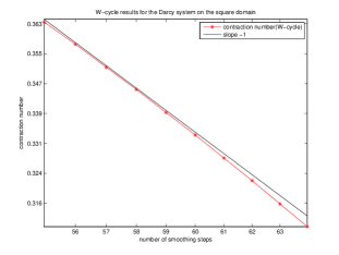
Figure 7.1. Contraction numbers of the $W$-cycle multigrid method for (7.1) on the unit square

We also report the contraction numbers of the $V$-cycle algorithm for (7.1) and (7.2) in Table 7.7 and Table 7.8. They are similar to the contraction numbers for the $W$-cycle algorithm in Table 7.5 and Table 7.6 but are slightly larger.

Table 7.7. Contraction numbers of the $V$-cycle multigrid method for (7.1) on the unit square

	$k=1$	$k=2$	$k=3$	$k=4$	$k=5$	$k=6$
$m=10$	0.80	0.82	0.81	0.82	0.82	0.82
$m=20$	0.66	0.68	0.68	0.68	0.68	0.68
$m=40$	0.47	0.48	0.48	0.48	0.48	0.48
$m=80$	0.24	0.25	0.25	0.25	0.25	0.25

Table 7.8. Contraction numbers of the $V$-cycle multigrid method for (7.2) on the unit square

	$k=1$	$k=2$	$k=3$	$k=4$	$k=5$	$k=6$
$m=10$	0.80	0.82	0.82	0.82	0.82	0.82
$m=20$	0.67	0.68	0.68	0.68	0.68	0.68
$m=40$	0.48	0.49	0.49	0.49	0.49	0.49
$m=80$	0.24	0.25	0.25	0.25	0.25	0.25

7.2.2. $L$-Shaped Domain

The contraction numbers of the $W$-cycle algorithms for (7.1) and (7.2) for various $m$ and $k=1,\ldots,6$ are displayed in Table 7.9 and Table 7.10. The contraction numbers are larger than the corresponding contraction numbers for the unit square, which is consistent with Theorem 5.4 and Theorem 6.8 since the index of elliptic regularity $\alpha$ for the $L$-shaped domain is less than $\frac{2}{3}$. This is also confirmed by the log-log graph in Figure 7.2, where the contraction number of the $W$-cycle algorithm for (7.1) is plotted against the number of smoothing steps $m$.

The contraction numbers for the $V$-cycle algorithm are similar and therefore not reported.

Table 7.9. Contraction numbers of the $W$-cycle multigrid method for (7.1) on the $L$-shaped domain

	$k=1$	$k=2$	$k=3$	$k=4$	$k=5$	$k=6$
$m=10$	0.81	0.82	0.82	0.82	0.82	0.82
$m=20$	0.70	0.70	0.70	0.70	0.70	0.70
$m=40$	0.51	0.51	0.51	0.51	0.51	0.51
$m=80$	0.28	0.28	0.28	0.28	0.28	0.28

Table 7.10. Contraction numbers of the $W$-cycle multigrid method for (7.2) on the $L$-shaped domain

	$k=1$	$k=2$	$k=3$	$k=4$	$k=5$	$k=6$
$m=10$	0.81	0.82	0.82	0.82	0.82	0.82
$m=20$	0.70	0.70	0.70	0.70	0.70	0.70
$m=40$	0.52	0.52	0.52	0.52	0.52	0.52
$m=80$	0.29	0.29	0.29	0.29	0.29	0.29

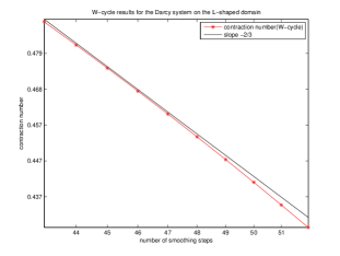
Figure 7.2. Contraction numbers of the $W$-cycle multigrid method for (7.1) on the $L$-shaped domain

8. Concluding Remarks

In this paper we developed multigrid algorithms for the Darcy system discretized by Raviart-Thomas-Nédélec mixed finite element methods of order at least 1, and showed that with minimal modifications the multigrid algorithms can also be applied to convection-diffusion-reaction and advection-diffusion-reaction problems. Note that the number of degrees of freedom of the Raviart-Thomas-Nédélec mixed finite element method of order 1 associated with a triangulation $\mathcal{T}_{h}$ is less than the number of degrees of freedom of the Raviart-Thomas-Nédélec mixed finite element method of order 0 associated with the triangulation $\mathcal{T}_{h/2}$ obtained from $\mathcal{T}_{h}$ by uniform refinement. Therefore, from the point of view of multigrid, the requirement that the order of the method has to be at least 1 is not restrictive.

The results in this paper can be extended to rectangular Raviart-Thomas-Nédélec mixed finite element methods and to other stable mixed finite element methods for the Darcy system. It should also be possible to extend our approach to mixed finite element methods for linear elasticity that are based on a stress-displacement formulation (cf. [10] and the references therein). We note that a nonstandard analysis similar to the one in Section 5 has been carried out in [42] for a family of such finite element methods.

Finally it would be interesting to extend our approach to the upwind mixed finite element methods for convection dominated problems in [32] (cf. also [33]).

Acknowledgement  The authors would like to thank Monique Dauge for helpful discussions on the regularity of the Darcy system.

References

- [1] M. B. Allen, R.E. Ewing, and P. Lu. Well-conditioned iterative schemes for mixed finite-element models of porous-media flows. SIAM J. Sci. Statist. Comput., 13:794–814, 1992.
- [2] P.F. Antonietti and B. Ayuso de Dios. Schwarz domain decomposition preconditioners for discontinuous Galerkin approximations of elliptic problems: non-overlapping case. M2AN Math. Model. Numer. Anal., 41:21–54, 2007.
- [3] D.N. Arnold and F. Brezzi. Mixed and nonconforming finite element methods: implementation, postprocessing and error estimates. R.A.I.R.O Modél. Math. Anal. Numér., 19:7–32, 1985.
- [4] D.N. Arnold, F. Brezzi, B. Cockburn, and L.D. Marini. Unified analysis of discontinuous Galerkin methods for elliptic problems. SIAM J. Numer. Anal., 39:1749–1779, 2001/02.
- [5] I. Babuška, J. Osborn, and J. Pitkäranta. Analysis of mixed methods using mesh dependent norms. Math. Comp., 35:1039–1062, 1980.
- [6] I. Babuška. The finite element method with Lagrange multipliers. Numer. Math., 20:179–192, 1973.
- [7] R.E. Bank and T.F. Dupont. An optimal order process for solving finite element equations. Math. Comp., 36:35–51, 1981.
- [8] F. Ben Belgacem and S.C. Brenner. Some nonstandard finite element estimates with applications to 3D Poisson and Signorini problems. Electron. Trans. Numer. Anal., 12:134–148, 2001.
- [9] M. Benzi, G.H. Golub, and J. Liesen. Numerical solution of saddle point problems. Acta Numerica, 14:1–137, 2005.
- [10] D. Boffi, F. Brezzi, and M. Fortin. Mixed Finite Element Methods and Applications. Springer, Heidelberg, 2013.
- [11] J.H. Bramble and S.R. Hilbert. Estimation of linear functionals on Sobolev spaces with applications to Fourier transforms and spline interpolation. SIAM J. Numer. Anal., 7:113–124, 1970.
- [12] J.H. Bramble and J. Xu. Some estimates for a weighted projection. Math. Comp., 56:463–476, 1991.
- [13] J.H. Bramble and X. Zhang. The Analysis of Multigrid Methods. In P.G. Ciarlet and J.L. Lions, editors, Handbook of Numerical Analysis, VII, pages 173–415. North-Holland, Amsterdam, 2000.
- [14] S.C. Brenner. A multigrid algorithm for the lowest-order Raviart-Thomas mixed triangular finite element method. SIAM J. Numer. Anal., 29:647–678, 1992.
- [15] S.C. Brenner. Convergence of nonconforming multigrid methods without full elliptic regularity. Math. Comp., 68:25–53, 1999.
- [16] S.C. Brenner. Poincaré-Friedrichs inequalities for piecewise functions. SIAM J. Numer. Anal., 41:306–324, 2003.
- [17] S.C. Brenner, H. Li, and L.-Y. Sung. Multigrid methods for saddle point problems Stokes and Lamé systems. Numer. Math., published online January 2014. (DOI: 10.1007/s00211-014-0607-3).
- [18] S.C. Brenner and L. R. Scott. The Mathematical Theory of Finite Element Methods Third Edition. Springer-Verlag, New York, 2008.
- [19] S.C. Brenner and J. Zhao. Convergence of multigrid algorithms for interior penalty methods. Appl. Numer. Anal. Comput. Math., 2:3–18, 2005.
- [20] F. Brezzi. On the existence, uniqueness and approximation of saddle-point problems arising from Lagrangian multipliers. RAIRO Anal. Numér., 8:129–151, 1974.
- [21] P.G. Ciarlet. The Finite Element Method for Elliptic Problems. North-Holland, Amsterdam, 1978.
- [22] M. Crouzeix and P.-A. Raviart. Conforming and nonconforming finite element methods for solving the stationary Stokes equations I. RAIRO Anal. Numér., 7:33–75, 1973.
- [23] M. Dauge. Elliptic Boundary Value Problems on Corner Domains, Lecture Notes in Mathematics 1341. Springer-Verlag, Berlin-Heidelberg, 1988.
- [24] J. Douglas, Jr. and J.E. Roberts. Mixed finite element methods for second order elliptic problems. Mat. Apl. Comput., 1:91–103, 1982.
- [25] T. Dupont and R. Scott. Polynomial approximation of functions in Sobolev spaces. Math. Comp., 34:441–463, 1980.
- [26] R. Ewing and J. Wang. Analysis of multilevel decomposition iterative methods for mixed finite element methods. Math. Modelling and Numer. Anal., 28:377–398, 1994.
- [27] R.S. Falk and J.E. Osborn. Error estimates for mixed methods. RAIRO Anal. Numér., 14:249–277, 1980.
- [28] X. Feng and O.A. Karakashian. Two-level additive Schwarz methods for a discontinuous Galerkin approximation of second order elliptic problems. SIAM J. Numer. Anal., 39:1343–1365, 2001.
- [29] J. Gopalakrishnan and G. Kanschat. A multilevel discontinuous Galerkin method. Numer. Math., 95:527–550, 2003.
- [30] P. Grisvard. Elliptic Problems in Non Smooth Domains. Pitman, Boston, 1985.
- [31] W. Hackbusch. Multi-grid Methods and Applications. Springer-Verlag, Berlin-Heidelberg-New York-Tokyo, 1985.
- [32] J. Jaffré. Décentrage et éléments finis mixtes pour les équations de diffusion-convection. Calcolo, 21:171–197, 1984.
- [33] D. Kim and E.-J. Park. A posteriori error estimators for the upstream weighting mixed methods for convection diffusion problems. Comput. Methods Appl. Mech. Engrg., 197:806–820, 2008.
- [34] C. Lasser and A. Toselli. An overlapping domain decomposition preconditioner for a class of discontinuous Galerkin approximations of advection-diffusion problems. Math. Comp., 72:1215–1238, 2003.
- [35] K.-A. Mardal and R. Winther. Preconditioning discretizations of systems of partial differential equations. Numer. Linear Algebra Appl., 18:1–40, 2011.
- [36] S.A. Nazarov and B.A. Plamenevsky. Elliptic Problems in Domains with Piecewise Smooth Boundaries. de Gruyter, Berlin-New York, 1994.
- [37] J.-C. Nédélec. Mixed finite elements in . Numer. Math., 35:315–341, 1980.
- [38] P.-A. Raviart and J.M. Thomas. A mixed finite element method for second order elliptic problems. In I.Galligani and E. Magenes, editors, Mathematical Aspects of the Finite Element Method, Lecture Notes in Mathematics 606, pages 292–315. Springer-Verlag, Berlin, 1977.
- [39] T. Rusten, P.S. Vassilevski, and R. Winther. Interior penalty preconditioners for mixed finite element approximations of elliptic problems. Math. Comp., 65:447–466, 1996.
- [40] T. Rusten and R. Winther. A preconditioned iterative method for saddlepoint problems. SIAM J. Matrix Anal. Appl., 13:887–904, 1992. Iterative methods in numerical linear algebra (Copper Mountain, CO, 1990).
- [41] A. Schatz. An observation concerning Ritz-Galerkin methods with indefinite bilinear forms. Math. Comp., 28:959–962, 1974.
- [42] R. Stenberg. A family of mixed finite elements for the elasticity problem. Numer. Math., 53:513–538, 1988.
- [43] L. Tartar. An Introduction to Sobolev Spaces and Interpolation Spaces. Springer, Berlin, 2007.
- [44] P.S. Vassilevski. Multilevel block factorization preconditioners. Springer, New York, 2008.