University of Oxford
11email: bernard@robots.ox.ac.uk, philip.torr@eng.ox.ac.uk
Recurrent Instance Segmentation
Abstract
Instance segmentation is the problem of detecting and delineating each distinct object of interest appearing in an image. Current instance segmentation approaches consist of ensembles of modules that are trained independently of each other, thus missing opportunities for joint learning. Here we propose a new instance segmentation paradigm consisting in an end-to-end method that learns how to segment instances sequentially. The model is based on a recurrent neural network that sequentially finds objects and their segmentations one at a time. This net is provided with a spatial memory that keeps track of what pixels have been explained and allows occlusion handling. In order to train the model we designed a principled loss function that accurately represents the properties of the instance segmentation problem. In the experiments carried out, we found that our method outperforms recent approaches on multiple person segmentation, and all state of the art approaches on the Plant Phenotyping dataset for leaf counting.
Keywords:
Instance segmentation, recurrent neural nets, deep learning1 Introduction
Instance segmentation, the automatic delineation of different objects appearing in an image, is a problem within computer vision that has attracted a fair amount of attention. Such interest is motivated by both its potential applicability to a whole range of scenarios, and the stimulating technical challenges it poses.
Regarding the former, segmenting at the instance level is useful for many tasks, ranging from allowing robots to segment a particular object in order to grasp it, to highlighting and enhancing the outline of objects for the partially sighted, wearing “smart specs” [1]. Counting elements in an image has interest in its own right [2] as it has a wide range of applications. For example, industrial processes that require the number of elements produced, knowing the number of people who attended a demonstration, and counting the number of infected and healthy blood cells in a blood sample, required in some medical procedures such as malaria detection [3].
Instance segmentation is more challenging than other pixel-level learning problems such as semantic segmentation, which deals with classifying each pixel of an image, given a set of classes. There, each pixel can belong to a set of predefined groups (or classes), whereas in instance segmentation the number of groups (instances) is unknown a priori. This difference exacerbates the problem: where in semantic segmentation one can evaluate the prediction pixel-wise, instance segmentation requires the clustering of pixels to be evaluated with a loss function invariant to the permutation of this assignment (i.e. it does not matter if a group of “person” pixels is assigned to be person “1” or person “2”). That leads to further complexities in the learning of these models. Hence, instance segmentation has remained a more difficult problem to solve.
Most approaches proposed for instance level segmentation are based on a pipeline of modules whose learning process is carried out independent of each other. Some of them, such as [4, 5], rely on a module for object proposal, followed by another one implementing object recognition and segmentation on the detected patches. A common problem with such piecewise learning methods is that each module does not learn to accommodate itself to the outputs of other modules. Another drawback is that in such cases, it is often necessary to define an independent loss function for each module, which places a burden on the practitioner to decide on convenient representations of the data at intermediate stages of the pipeline.
These issues led us to take a different route and develop a fresh and end-to-end model able to learn the whole instance-segmentation process. Due to the magnitude of the task, in this study we focus on the problem of class-specific instance segmentation. That is, we assume that the model segments instances that belong to the same class, excluding classification stages. The solution to this problem is useful in its own right, for example to segment and to count people in images [6], but we consider that this is also the first step towards general semantic learning systems that can segment and classify different kinds of instances.

The approach we propose here is partially inspired by how humans count elements in a scene. It is known, [7, 8], that humans count sequentially, using accurate spatial memory in order to keep track of the accounted locations. Driven by this insight, our purpose is to build a learning model capable of segmenting the instances of an object in an image sequentially, keeping the current state in an internal memory. In order to achieve this, we rely on recurrent neural networks (RNNs), which exhibit the two properties discussed: the ability to produce sequential output, and the ability to keep a state or memory along the sequence.
Our primary contributions, described in this paper, are 1. the development of an end-to-end approach for class specific instance segmentation, schematized in Fig (1), based on RNNs containing convolutional layers, and 2. the derivation of a principled loss function for this problem. We assess the capabilities of our model by conducting two experiments; one on segmentation of multiple people, and the other on plant-leaves segmentation and counting.
2 Background
The work presented here combines several research areas. In this section we summarize the main developments in these areas.
2.1 Instance Segmentation Models
Instance segmentation can be formulated as the conjunction between semantic segmentation and object detection, for example in [9], the authors proposed a model that integrates information obtained at pixel, segment, and object levels. This is because instance segmentation requires the capacity of object detection approaches to separate between instances, and the ability of semantic segmentation methods to produce pixel-wise predictions, and hence a delineation of the shape of the objects. The progress of instance segmentation methods is thus limited by the advances made in both object detection and semantic segmentation.
A recent breakthrough in object detection is the Region-based CNN (R-CNN) [10]. This approach consists in using a region proposal method to produce a large set of varied sized object proposals from an image, then extracting features for each of them by means of a CNN, and finally classifying the resultant feature vectors. Several approaches for instance segmentation build on this method. Two of them are [4, 5], which both use multiscale combinatorial grouping [11] as a region proposal method to extract candidates, followed by a region refinement process. In the former work [4], the authors perform non-maximum suppression on the candidates, in order to remove duplicates, and then they combine the coarse information obtained by the CNN with superpixels extracted from the image in order to segment the instances. In the latter work [5], the output is refined by means of exemplar-based shape prediction and graph-cut. These approaches have produced state of the art results in instance segmentation. However, they suffer a common drawback that we want to avoid: they consist in an ensemble of modules that are trained independently of each other.
Semantic segmentation methods have seen a significant improvement recently, based first on the work in [12] which proposed a fully convolutional network that produces pixel-wise predictions, followed by the works in [13, 14] that improve the delineation of the predicted objects by using Conditional Random Fields (CRFs). The work in [15] builds an instance segmentation model standing on these previous approaches. This is based on predicting pixel-wise instances locations by a network, and then applying a clustering method as a post-processing step, where the number of clusters (instances) is predicted by another CNN. A problem with this approach is that it is not optimizing a direct instance segmentation measure, but it relies on a surrogate loss function based on pixel distances to object positions.
One problem associated to instance segmentation is related to the lack of an order among the instances in images (e.g. which instance should be the first to be segmented). Several works [16, 17, 18] aim to overcome this problem by inferring and exploiting depth information as a way to order the instances. They model that by means of a Markov Random Field on the top of a CNN. One advantage of this approach is that occlusion between objects is explicitly modeled. A disadvantage is that this approach is not beneficial when instances appear at a similar depth, for example, an image containing a sport team with many players together.
Unlike previous approaches, we propose a new paradigm for instance segmentation based on learning to segment instances sequentially, letting the model decide the order of the instances for each image.
2.2 Recurrent Neural Networks
Recurrent neural networks (RNNs) are powerful learning models. Their power resides in their capacity to keep a state or memory, in which the model is able to store what it considers relevant events towards minimizing a given loss function. They are also versatile, as they can be applied to arbitrary input and output sequence sizes. These two properties have led to the successful application of RNNs to a wide range of tasks such as machine translation [19], handwriting recognition [20] and conversational models [21], among others.
RNNs are also useful for obtaining variable length information from static images. One such example is DRAW [22], which is a variational auto-encoder for learning how to generate images, in which both the encoder and the decoder are RNNs, so that the image generation process is sequential. Image captioning is another application which has benefited from the use of RNNs on images. Examples of these are [23, 24, 25], which are based on using a CNN for obtaining a meaningful representation of the image, which is then introduced into an RNN that produces one word at each iteration. Another example, involving biological images, is in [26], where the authors explore a combination of convolutional layers and LSTMs in order to predict for each protein the subcellular compartment it belongs to. In [27] the authors use an RNN to predict a bounding box delimiting one human face at each iteration. This approach shares some of our motivations. The main difference between both approaches is that in [27] they consider a regression problem, producing at each iteration a set of scalars that specify the bounding box where the instance is, whereas we consider a pixel-wise classification problem. In [28], the authors present several recurrent structures to track and segment objects in videos. Finally, it is worth mentioning the approach in [29] despite not being an RNN, which consists in a greedy sequential algorithm for learning several objects in an image.
2.3 Attention Based Models
Attention based approaches consist in models that have the capability of deciding at each time which part of the input to look at in order to perform a task. They have recently shown impressive performance in several tasks like image generation [22], object recognition [30], and image caption generation [31]. These approaches can be divided into two main categories: hard, and soft attention mechanisms. Hard attention mechanisms are those that decide which part of the instance process at a time, totally ignoring the remainder [32]. On the contrary, soft attention mechanisms decide at each time a probability distribution over the input, indicating the attention that each part must receive. The latter are wholly differentiable, thus they can be optimized by backpropagation [33].
Our approach resembles attention models in the sense that in both cases the model selects different parts of the same input in successive iterations. Attention based models are different from our approach in which they apply attention mechanisms as a means to an end task (e.g. image caption generation or machine translation), whereas in our approach, attention to one instance at each time is the end target we aim for.
3 Segmenting One Instance at a Time
In this section we describe the inference process that our approach performs, as well as the structural elements that compose it.
The process at inference stage is depicted in Fig (1), and can be described as follows: an image with height and width , ( is usually , or if including depth information) is taken as input of a fully convolutional network, such as the one described in [12]. This is composed of a sequence of convolutional and max-pooling layers that preserve the spatial information in the inner representations of the image. The output of that network, , represents the -dimensional features extracted for each pixel, where the size of this map may be smaller than the size of the input image, , , due to the subsampling effect of the described network. This output will be the input to the RNN in all iterations in the sequence. At the beginning of the sequence, the initial inner state of the RNN, , is initialized to . After the first iteration, the RNN produces the segmentation of one of the instances in the image (any of them), together with an indicator that informs about the confidence of the prediction in order to have a stopping condition. Simultaneously, the RNN updates the inner state, , to account for the recent segmented instance. Then, having again as inputs , and as inner state , the model outputs another segmented instance and its confidence score. This process keeps iterating until the confidence score drops below a certain level in which the model stops, ideally having segmented all instances in the image.
The sequential nature of our model allows to deal with common instance segmentation problems. In particular it can implicitly model occlusion, as it can segment non-occluded instances first, and keep in its state the regions of the image that have already been segmented in order to detect occluded objects. Another purpose of the state is to allow the model to consider potential relationships from different instances in the image. For example, if in the first iteration an instance of a person embracing something is segmented, and this information is somehow kept in the state, then in subsequent iterations, it might increase the plausibility of having another person being embraced by the first one.
The structure of our approach is composed of a fully convolutional network, followed by an RNN, a function to transform the state of the RNN into the segmentation of an instance and its confidence score, and finally the loss function that evaluates the quality of the predictions and that we aim to optimize. The first of these components, the fully convolutional network, is used in a similar manner as explained in [12]. In the following we describe in detail the remaining three components.
3.1 Convolutional LSTM
Long short-term memory (LSTM) networks [34] have stood out over other recurrent structures because they are able to prevent the vanishing gradient problem. Indeed, they are the chosen model in most works reviewed in Sec. 2.2 in which they have achieved outstanding results. In this section we build on top of the LSTM unit, but we perform some changes in its structure to adapt it to the characteristics of our problem.
In the problem we have described, we observe that the input to the model is a map from a lattice (in particular, an image), and the output is also a map from a lattice. Problems with these characteristics, such as semantic segmentation [12, 14] and optical flow [35], are often tackled using structures based on convolutions, in which the intermediate representations of the images preserve the spatial information. In our problem, we can see the inner state of recurrent units as a map that preserves spatial information as well. That led us to convolutional versions of RNNs, and in particular to convolutional long short-term memory (ConvLSTM) units.
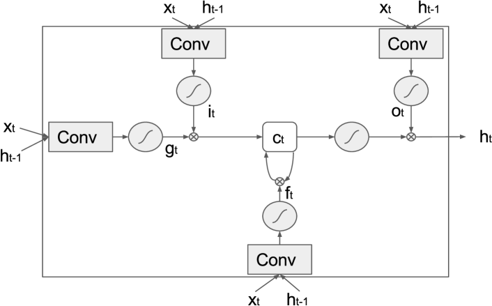
A ConvLSTM unit is similar to an LSTM one, the only difference being that the fully connected layers in each gate are replaced by convolutions, as specified by the following update equations:
| (1) |
where represents the element-wise product operator, are the gates, and represents the memory of the recurrent unit, being the amount of memory used for each pixel (in this paper we assume that the number of channels in the recurrent unit is the same as the number of channels produced by the previous FCN). Each of the filter weights ( terms) has dimensionality , where is the size of the filter, and each of the bias terms ( terms) is a -dimensional vector repeated across height and width. We refer to the diagrams and definitions presented in [34] for a detailed explanation of the LSTM update equations, from which eq. (1) follows. We also provide a diagram illustrating eq. (1) in the Appendix Sec. B. Note that a primary aspect of keeping a memory or state is to allow our model to keep account of the pixels of the image that have already been segmented in previous iterations of the process. This can be naturally done by applying convolutions to the state. We can also stack two or more ConvLSTM units with the aim of learning more complex relationships.
The advantages of ConvLSTM with respect to regular LSTM go hand in hand with the advantages of convolutional layers with respect to linear layers: they are suitable for learning filters, useful for spatially invariant inputs such as images, and they require less memory for the parameters. In fact the memory required is independent of the size of the input. A similar recurrent unit has been recently proposed in [36] in the context of weather forecasting in a region.
3.2 Attention by Spatial Inhibition
The output produced by our model at time is a function of the hidden state, . This function produces two outputs, . The first output is a map that indicates which pixels compose the object that is segmented in the current iteration. The second output is the estimated probability that the current segmented candidate is an object. We use this output as a stopping condition. In the following we describe these two functions, supporting our presentation on a schematic view of , which is given in Fig. (2).
The function that produces the first output can be described as a sequence of layers which have the aim of discriminating one, and only one instance, filtering out everything else. Firstly we use a convolutional layer which maps the channels of the hidden state to output channel, using filters. This is followed by a log-softmax layer, , which normalizes the input across all pixels, and then applies a logarithm. As a result, each pixel value can be in the interval , where the sum of the exponentiation of all values is . This leads to a competing mechanism that has the potential of inhibiting pixels that do not belong to the current instance being segmented. Following that, we use a layer which adds a learned bias term to the input data. The purpose of this layer is to learn a threshold, , which filters the pixels that will be selected for the present instance. Then, a sigmoid transformation is applied pixel-wise. Hence, the resultant pixel values are all in the interval , as required. Finally, we upsample the resultant map back to the original size of the input image, . In order to help understand the effect of these layers, we visualize in Sec. A in the Appendix, the inner representations captured by the model at different stages of the described pipeline.

The function which encodes the relationship between the current state and the confidence of the predicted candidate consists simply of a max-pooling and a linear layer, followed by a sigmoid function.
3.3 Loss Function
Choosing a loss function that accurately reflects the objective we want to achieve is key for any model to be able to learn a given task. In order to present the loss function that we use, let us first add some notation.
At training stage we are provided with the training set composed of labeled images. We denote image as , where for simplicity we consider the same size () for all images. Its annotation , is a set of masks, , for , containing the segmentation of each instance in the image. One point to note about the labels is that the dimension of the last index, , depends on the image , because each image may have a different number of instances.
Our model predicts both a sequence of masks, , for image , where , , and a confidence score associated to those masks . At inference time, the number of elements predicted, , depends on the confidence values, , so that the network stops producing outputs after time when . At training time we can predefine the length of the predicted sequence. Given that we know the length, , of the -th ground truth annotation, we set the length of the predicted sequence to be , so that the network can learn when to stop. In any case, the number of elements in the predicted sequence, , is not necessarily equal to the elements in the corresponding ground truth set, , given that our model could underestimate or overestimate the number of objects.
One way to represent the scenario is to arrange the elements in and (where we omit hereafter the index of the image, , for the sake of clarity) in a bipartite graph, in which each edge between , , and , , has a cost associated to the intersection over union between and . A similarity measure between and can be defined as the maximum sum of the intersection over union correspondence between the elements in and the elements in :
| (2) |
where
| (3) |
| (4) |
, used in [37], is a relaxed version of the intersection over union (IoU) that allows the input to take values in the continuous interval , and , so that function (3) only accounts for the first predicted masks, ignoring the remainder in case our model produces more instances.
The elements in determine the optimal matching between the elements in and , so that is assigned to if and only if . The constraint set , defined in eq. (4), impedes one ground truth instance being assigned to more than one of the predicted instances and vice versa. It may be the case that the ground truth is not covered by any prediction if and only if . The optimal matching, , can be found out efficiently by means of the Hungarian algorithm, in a similar vein as in [27]. The coverage loss described in [38] has a similar form, where the predictions were discrete, and the problem was posed as an integer program.
End-to-end learning is possible with this loss function, as it is the point-wise minimum of a set of continuous functions (each of those functions corresponding to a possible matching in ). Thus, a direction of decrease of the loss function at a point can be computed by following two steps: 1. Figuring out which function in the set achieves the minimum at that point. 2. Computing the gradient of that function. Here, the Hungarian algorithm is employed in the described first step to find out the function that achieves the minimum at the point. Then, the gradient of that function is computed. The details of this process are shown in Sec. D in the Appendix.
We now need to account for the confidence scores predicted by the model. To do so, we consider that the ideal output is to predict if the number of instances segmented so far is equal or less than the total number of instances , otherwise should be . Taking this into account, we propose the following loss function:
| (5) |
where is the binary cross entropy, and the Iverson bracket is if the condition within the brackets is true, and otherwise. Finally, is a hyperparameter that ponders the importance of the second term with respect to the first one.
4 Experiments
We perform two kinds of experiments, in which we study the capabilities of our approach to both segment and count instances. In the first experiment we focus on multi-instance subject segmentation, and in the second we focus on segmenting and counting leaves in plants. Before presenting those results, we first describe the implementations details that are common to both experiments.
4.1 Implementation Details of our Method
We have implemented our approach using the Lua/Torch deep learning framework [39]. The code and models are publicly available111Available at http://romera-paredes.com/ris..
The recurrent stage is composed of two ConvLSTM layers, so that the output of the first ConvLSTM acts as the input for the second one. This stage is followed by the spatial inhibition module which produces a confidence score together with an instance segmentation mask. The resultant prediction is evaluated according to the loss function defined in eq. (5), where we set .
At training stage, the parameters of the recurrent structure are learned by backpropagation through time. In order to prevent the exploding gradient effect, we clipped the gradients so that each of its elements has a maximum absolute value of . We use the Adam optimization algorithm [40] for training the whole network, setting the initial learning rate to , and multiplying it by when the training error plateaus. We use neither dropout nor regularization, as we did not observe overfitting in preliminary experiments. In the same way as in [14], we have used one image per batch.
The weights of the recurrent structure are initialized at random, sampling them uniformly from the interval with the exception of the bias terms in the forget gate, in eq. (1). They have been initialized to with the aim of allowing by default to backpropagate the error to previous iterations in the sequence.
We perform curriculum learning by gradually increasing the number of objects that are required to be segmented from the images. That is, at the beginning we use only recurrent iterations, so that the network is expected to learn to extract at most objects per image, even when there are more. Once the training procedure converges, we increment this number, and keep iterating the process.
At inference time we assign a pixel to an instance if the predicted value is higher than . Nevertheless, we observe that the predicted pixels values in are usually saturated, that is, they are either very close to or very close to . Although uncommon, it might happen that the same pixel is assigned to more than one instance in the sequence. Whenever that is the case, we assign the pixel to the instance belonging to the earlier iteration. Finally, the produced sequence terminates whenever the confidence score predicted by the network is below .
4.2 Multiple Person Segmentation
We assess the quality of our approach for detecting and segmenting individual subjects in real images. Multiple person segmentation is extremely challenging because people in pictures present high variations such as different posture, age, gender, clothing, location and depth within the scene, among others.
In order to learn this task, we have integrated our model on the FCN-8s network developed in [12]. The FCN-8s network is composed of a series of layers and adding skips that produce, as a result, an image representation whose size is smaller than the original image. This is followed by an upsampling layer that resizes the representation back to the original image size. We modify this structure by putting the ConvLSTM before this upsampling layer, which is integrated into the subsequent spatial inhibition module, as shown in Fig. 2. Following other works such as [12, 14] we add padding and/or resize the input image so that the resultant size is . As a consequence, the size of the input of the ConvLSTM layers, as well as their hidden states have dimensionality , where is the number of features extracted for each pixel. All gates (, , , and in eq. 1) of both ConvLSTM layers use convolutions.
For training we used the MSCOCO dataset [41], and the training images of the Pascal VOC 2012 dataset. We first fixed the weights of the FCN-8s except for the last layer, and then learned the parameters of that last layer, together with the ConvLSTM and the spatial inhibition module, following the procedure described in Sec. 4.1. Then we fine-tuned the whole network using a learning rate of until convergence.
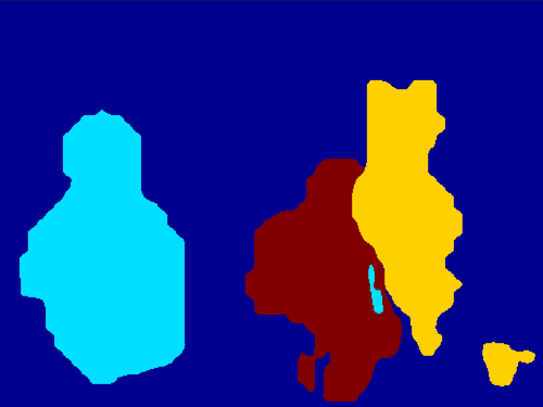
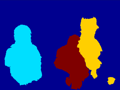
We observed that the predictions obtained by recurrent instance segmentation (RIS), while promising, were coarse with respect to the boundaries of the segmented subjects. That is expected, as the ConvLSTM operates on a low resolution representation of the image. In order to amend this, we have used a CRF as a post-processing method over the produced segments. We call this approach RIS+CRF.
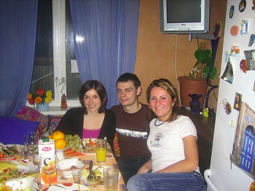
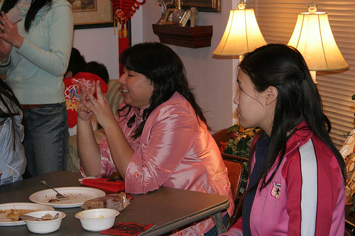
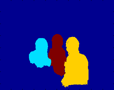
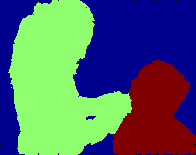
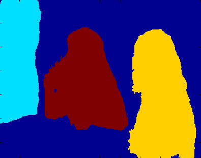
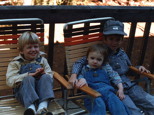
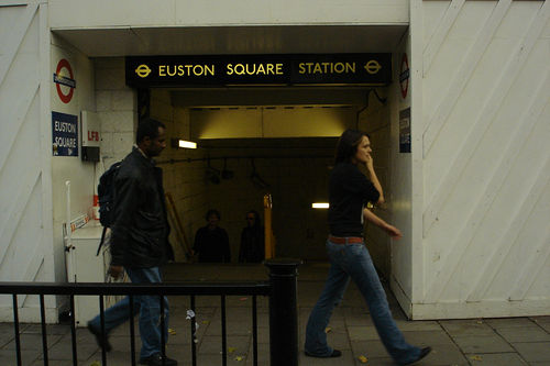
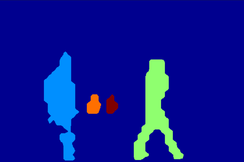
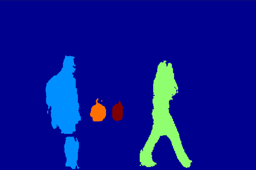
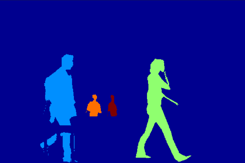
We compare these two approaches with the recent instance segmentation methods presented in [5, 4, 15], already introduced in Sec. 2.1. We also compare to a baseline consisting in performing proposal generation from the semantic segmentation result produced by the FCN-8s of [12]. We have used Faster R-CNN [42] as the proposal generation method. Following previous works, we measure the predictive performance of the methods with respect to the Pascal VOC 2012 validation set, using two standard metrics: average precision () on the predicted regions having over IoU overlapping with ground truth masks, denoted as ; and averaging the for different degrees of IoU overlapping, from to , denoted as . We show the results in Table 1. We observe that RIS achieves comparable results to state of the art approaches. When using CRF as a post-processing method the results improve, outperforming the competing methods. We also provide some qualitative results in Fig. 3, and more extensively in Sec. C in the Appendix.
| Baseline | [5] | [4] | [15] | RIS | RIS+CRF | |
 |
 |
 |
 |
 |
 |
4.3 Plants Leaf Segmentation and Counting
Automatic leaf segmentation and counting are useful tasks for plant phenotyping applications that can lead to improvements in seed production and plant breeders processes. In this section we use the Computer Vision Problems in Plant Phenotyping (CVPPP) dataset [43, 44]. In particular, we utilize the A1 subset of plants, which is the biggest subset available, and contains top-down view images, having size each, as the one shown in Fig. (1, Left). The training set is composed of of those images, which have annotations available. The remaining images are left out for testing purposes. All these images are challenging because they present a high range of variations, with occasional leaf occlusions, varied backgrounds, several slightly blurred images due to a lack of focus, and complex leaf shapes.
The limited number of training images has driven us to augment the data by considering some valid transformations of the images. We apply two transformations: rotating the image by a random angle, and flipping the resultant image with a probability of .
We learn the fully convolutional network from scratch. Its structure is composed by a sequence of convolutional layers, each of them followed by a rectified linear unit. The first convolution learns filters, and the following four learn filters each. This sequence of convolutions produces a representation of the image, which is the input to the recurrent stage of the model. In the stack of two ConvLSTMs we have set all gates to have convolutional layers.
We compare our method with several approaches submitted to the CVPPP challenges on both leaf segmentation and counting. These are:
-
•
IPK Gatersleben [45]: Firstly, it segments foreground from background by using 3D histograms and a supervised learning model. Secondly, it identifies the leaves centre points and leaves split points by applying unsupervised learning methods, and then it segments individual leaves by applying graph-based noise removal, and region growing techniques.
-
•
Nottingham [46]: Firstly, SLIC is applied on the image in order to get superpixels. Then the plant is extracted from the background. The superpixels in the centroids of each leaf are identified by finding local maxima on the distance map of the foreground. Finally, leaves are segmented by applying the watershed transform.
- •
-
•
Wageningen [48]: It performs foreground segmentation using a neural network, followed by a series of image processing transformations, including inverse distance image transform from the detected foreground, and using the watershed transform to segment leaves individually.
-
•
PRIAn [49]: First, a set of features is learned in an unsupervised way on a log-polar representation of the image. Then, a support vector regression model is applied on the resultant features in order to predict the number of leaves.
These competing methods are explicitly designed to perform well in this particular plant leaf segmentation and counting problems, containing heuristics that are only valid on this domain. On the contrary, the applicability of our model is broad.
| IPK | Nottingham | MSU | Wageningen | PRIAn | RIS | RIS+CRF | |
|---|---|---|---|---|---|---|---|
The results obtained are shown in Table 2, using the measures reported by the CVPPP organization in order to compare the submitted solutions. These are Difference in Count () which is the difference between the predicted number of leaves and the ground truth, , which is the absolute value of DiC averaged across all images, and Symmetric Best Dice (), which is defined in [46], and provides a measure about the accuracy of the segmentation of the instances. Regarding leaf counting, we observe that our approach significantly outperforms the competing ad hoc methods that were designed for this particular problem. With regard to segmentation of leaves, our approach obtains comparable results with respect to the competitors, yet it does not outperform any approach. We hypothesize that despite the data augmentation process we follow, the amount of original images available for training is too small as to learn how to segment a wide variety of leaf shapes from scratch. This scarcity of training data has a smaller impact in the competing methods, given that they contain heuristics and prior information about the problem.
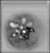
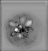
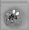
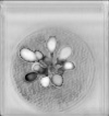
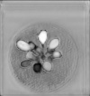
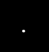
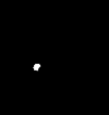
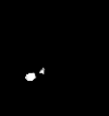
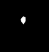
We have also visualized, in Fig. 4, a representation of what the network keeps in memory as the sequence is produced. The column denoted as shows a summary function of the hidden state of the second ConvLSTM layer. The summary function consists of the sum of the absolute values across channels for each pixel. The column denoted as corresponds to the output produced by the network. We observe that as time advances, the state is modified to take into account parts of the image that have been visited. We also inspected the value of the cell, that is in eq. (1), but we have not observed any clear clues.
 |
 |
 |
 |
 |
|
 |
 |
 |
 |
 |
5 Discussion
In this paper we have proposed a new instance segmentation paradigm characterized by its sequential nature. Similarly to what human beings do when counting objects in a scene, our model proceeds sequentially, segmenting one instance of the scene at a time. The resulting model integrates in a single pipeline all the required functions to segment instances. These functions are defined by a set of parameters that are jointly learned end-to-end. A key aspect in our model is the use of a recurrent structure that is able to track visited areas in the image as well as to handle occlusion among instances. Another key aspect is the definition of a loss function that accurately represents the instance segmentation objective we aim to achieve. The experiments carried out on multiple person segmentation and leaf counting show that our approach outperforms state of the art methods. Qualitative results show that the state in the recurrent stage contains information regarding the visited instances in the sequence.
The primary objective of this paper is to show that learning end-to-end instance segmentation is possible by means of a recurrent neural network. Nevertheless, variations of some architectural choices could lead to even better results. We tried a variety of other alternatives, such as adding the sum of the prediction masks as an extra input into the recurrent unit. We also tried alternatives to in eq. (3), such as log-likelihood. The results obtained in either case were not better than the ones achieved by the model described in Sec. 3. The analysis of these and other alternative architectures is left for future work.
There are several extensions that can be carried out in our approach. One is allowing the model to classify the segmented instance at each time. This can be done by generalizing the loss function in eq. (5). Another extension consists in integrating the CRF module as a layer in the end-to-end model, such as in [14]. Another interesting line of research is investigating other recurrent structures that could be as good or even better than ConvLSTMs for instance segmentation. Finally, the extension of this model for exploiting co-occurrence of objects, parts of objects, and attributes, could be a promising research direction.
Acknowledgments
This work was supported by the EPSRC, ERC grant ERC-2012-AdG 321162-HELIOS, HELIOS-DFR00200, EPSRC grant Seebibyte EP/M013774/1 and EPSRC/MURI grant EP/N019474/1.
Thanks to Siddharth Narayanaswamy for proofreading this work.
References
- [1] VA-ST: Smart specs. http://www.va-st.com/smart-specs
- [2] Arteta, C., Lempitsky, V., Noble, J.A., Zisserman, A.: Learning to detect partially overlapping instances. In: Computer Vision and Pattern Recognition (CVPR), IEEE (2013) 3230–3237
- [3] Trager, W., Jensen, J.B.: Human malaria parasites in continuous culture. Science 193(4254) (1976) 673–675
- [4] Hariharan, B., Arbeláez, P., Girshick, R., Malik, J.: Simultaneous detection and segmentation. In: European Conference on Computer Vision (ECCV). Springer (2014) 297–312
- [5] Chen, Y.T., Liu, X., Yang, M.H.: Multi-instance object segmentation with occlusion handling. In: Proceedings of the IEEE Conference on Computer Vision and Pattern Recognition (CVPR). (2015) 3470–3478
- [6] Vineet, V., Warrell, J., Ladicky, L., Torr, P.H.: Human instance segmentation from video using detector-based conditional random fields. In: British Machine Vision Conference (BMVC). (2011) 1–11
- [7] Dehaene, S., Cohen, L.: Dissociable mechanisms of subitizing and counting: neuropsychological evidence from simultanagnosic patients. Journal of Experimental Psychology: Human Perception and Performance 20(5) (1994) 958
- [8] Porter, G., Troscianko, T., Gilchrist, I.D.: Effort during visual search and counting: Insights from pupillometry. The Quarterly Journal of Experimental Psychology 60(2) (2007) 211–229
- [9] Ladickỳ, L., Sturgess, P., Alahari, K., Russell, C., Torr, P.H.: What, where and how many? combining object detectors and crfs. In: European Conference on Computer Vision (ECCV). Springer (2010) 424–437
- [10] Girshick, R., Donahue, J., Darrell, T., Malik, J.: Rich feature hierarchies for accurate object detection and semantic segmentation. In: Computer Vision and Pattern Recognition (CVPR), IEEE (2014) 580–587
- [11] Arbelaez, P., Pont-Tuset, J., Barron, J., Marques, F., Malik, J.: Multiscale combinatorial grouping. In: Computer Vision and Pattern Recognition (CVPR), 2014 IEEE Conference on, IEEE (2014) 328–335
- [12] Long, J., Shelhamer, E., Darrell, T.: Fully convolutional networks for semantic segmentation. In: Proceedings of the IEEE Conference on Computer Vision and Pattern Recognition (CVPR). (2015) 3431–3440
- [13] Liang-Chieh, C., Papandreou, G., Kokkinos, I., Murphy, K., Yuille, A.: Semantic image segmentation with deep convolutional nets and fully connected crfs. In: International Conference on Learning Representations (ICLR). (2015)
- [14] Zheng, S., Jayasumana, S., Romera-Paredes, B., Vineet, V., Su, Z., Du, D., Huang, C., Torr, P.H.: Conditional random fields as recurrent neural networks. IEEE International Conference on Computer Vision (ICCV) (2015)
- [15] Liang, X., Wei, Y., Shen, X., Yang, J., Lin, L., Yan, S.: Proposal-free network for instance-level object segmentation. arXiv preprint arXiv:1509.02636 (2015)
- [16] Tighe, J., Niethammer, M., Lazebnik, S.: Scene parsing with object instances and occlusion ordering. In: Computer Vision and Pattern Recognition (CVPR), IEEE (2014) 3748–3755
- [17] Yang, Y., Hallman, S., Ramanan, D., Fowlkes, C.C.: Layered object models for image segmentation. Pattern Analysis and Machine Intelligence, IEEE Transactions on 34(9) (2012) 1731–1743
- [18] Zhang, Z., Schwing, A.G., Fidler, S., Urtasun, R.: Monocular object instance segmentation and depth ordering with cnns. In: IEEE International Conference on Computer Vision (ICCV). (2015) 2614–2622
- [19] Bahdanau, D., Cho, K., Bengio, Y.: Neural machine translation by jointly learning to align and translate. arXiv preprint arXiv:1409.0473 (2014)
- [20] Graves, A., Schmidhuber, J.: Offline handwriting recognition with multidimensional recurrent neural networks. In: Advances in Neural Information Processing Systems (NIPS). (2009) 545–552
- [21] Vinyals, O., Le, Q.: A neural conversational model. arXiv preprint arXiv:1506.05869 (2015)
- [22] Gregor, K., Danihelka, I., Graves, A., Wierstra, D.: Draw: A recurrent neural network for image generation. Proceedings of the 32nd International Conference on Machine Learning (ICML) (2015)
- [23] Donahue, J., Anne Hendricks, L., Guadarrama, S., Rohrbach, M., Venugopalan, S., Saenko, K., Darrell, T.: Long-term recurrent convolutional networks for visual recognition and description. In: Proceedings of the IEEE Conference on Computer Vision and Pattern Recognition (CVPR). (2015) 2625–2634
- [24] Karpathy, A., Fei-Fei, L.: Deep visual-semantic alignments for generating image descriptions. In: Proceedings of the IEEE Conference on Computer Vision and Pattern Recognition (CVPR). (2015) 3128–3137
- [25] Vinyals, O., Toshev, A., Bengio, S., Erhan, D.: Show and tell: A neural image caption generator. In: Conference on Computer Vision and Pattern Recognition (CVPR). (2015) 3156–3164
- [26] Winther, O.: Convolutional lstm networks for subcellular localization of proteins. In: Algorithms for Computational Biology: Second International Conference, AlCoB 2015, Mexico City, Mexico, August 4-5, 2015, Proceedings. Volume 9199., Springer (2015) 68
- [27] Stewart, R., Andriluka, M.: End-to-end people detection in crowded scenes. arXiv preprint arXiv:1506.04878 (2015)
- [28] Pavel, M.S., Schulz, H., Behnke, S.: Recurrent convolutional neural networks for object-class segmentation of rgb-d video. In: International Joint Conference on Neural Networks (IJCNN), IEEE (2015) 1–8
- [29] Williams, C.K., Titsias, M.K.: Greedy learning of multiple objects in images using robust statistics and factorial learning. Neural Computation 16(5) (2004) 1039–1062
- [30] Ba, J., Mnih, V., Kavukcuoglu, K.: Multiple object recognition with visual attention. International Conference on Learning Representations (ICLR) (2015)
- [31] Xu, K., Ba, J., Kiros, R., Cho, K., Courville, A., Salakhudinov, R., Zemel, R., Bengio, Y.: Show, attend and tell: Neural image caption generation with visual attention. In: Proceedings of the 32nd International Conference on Machine Learning (ICML). (2015) 2048–2057
- [32] Mnih, V., Heess, N., Graves, A., et al.: Recurrent models of visual attention. In: Advances in Neural Information Processing Systems (NIPS). (2014) 2204–2212
- [33] Hermann, K.M., Kocisky, T., Grefenstette, E., Espeholt, L., Kay, W., Suleyman, M., Blunsom, P.: Teaching machines to read and comprehend. In: Advances in Neural Information Processing Systems (NIPS). (2015) 1693–1701
- [34] Hochreiter, S., Schmidhuber, J.: Long short-term memory. Neural computation 9(8) (1997) 1735–1780
- [35] Dosovitskiy, A., Fischery, P., Ilg, E., Hazirbas, C., Golkov, V., van der Smagt, P., Cremers, D., Brox, T., et al.: Flownet: Learning optical flow with convolutional networks. In: IEEE International Conference on Computer Vision (ICCV), IEEE (2015) 2758–2766
- [36] Xingjian, S., Chen, Z., Wang, H., Yeung, D.Y., Wong, W.k., Woo, W.c.: Convolutional lstm network: A machine learning approach for precipitation nowcasting. In: Advances in Neural Information Processing Systems (NIPS). (2015) 802–810
- [37] Krähenbühl, P., Koltun, V.: Parameter learning and convergent inference for dense random fields. In: Proceedings of the 30th International Conference on Machine Learning (ICML). (2013) 513–521
- [38] Silberman, N., Sontag, D., Fergus, R.: Instance segmentation of indoor scenes using a coverage loss. In: European Conference on Computer Vision (ECCV). Springer (2014) 616–631
- [39] Collobert, R., Kavukcuoglu, K., Farabet, C.: Torch7: A matlab-like environment for machine learning. In: BigLearn, NIPS Workshop. Number EPFL-CONF-192376 (2011)
- [40] Kingma, D., Ba, J.: Adam: A method for stochastic optimization. arXiv preprint arXiv:1412.6980 (2014)
- [41] Lin, T.Y., Maire, M., Belongie, S., Hays, J., Perona, P., Ramanan, D., Dollár, P., Zitnick, C.L.: Microsoft coco: Common objects in context. In: European Conference on Computer Vision (ECCV). Springer (2014) 740–755
- [42] Ren, S., He, K., Girshick, R., Sun, J.: Faster r-cnn: Towards real-time object detection with region proposal networks. In: Advances in neural information processing systems (NIPS). (2015) 91–99
- [43] Minervini, M., Abdelsamea, M.M., Tsaftaris, S.A.: Image-based plant phenotyping with incremental learning and active contours. Ecological Informatics 23 (2014) 35–48
- [44] Minervini, M., Fischbach, A., Scharr, H., Tsaftaris, S.A.: Finely-grained annotated datasets for image-based plant phenotyping. Pattern Recognition Letters (2015) Special Issue on Fine-grained Categorization in Ecological Multimedia.
- [45] Pape, J.M., Klukas, C.: 3-d histogram-based segmentation and leaf detection for rosette plants. In: Computer Vision-ECCV 2014 Workshops, Springer (2014) 61–74
- [46] Scharr, H., Minervini, M., French, A.P., Klukas, C., Kramer, D.M., Liu, X., Luengo Muntion, I., Pape, J.M., Polder, G., Vukadinovic, D., Yin, X., Tsaftaris, S.A.: Leaf segmentation in plant phenotyping: A collation study. Machine Vision and Applications (In print) (2015)
- [47] Barrow, H.G., Tenenbaum, J.M., Bolles, R.C., Wolf, H.C.: Parametric correspondence and chamfer matching: Two new techniques for image matching. Technical report, DTIC Document (1977)
- [48] Yin, X., Liu, X., Chen, J., Kramer, D.M.: Multi-leaf tracking from fluorescence plant videos. In: Image Processing (ICIP), 2014 IEEE International Conference on, IEEE (2014) 408–412
- [49] Giuffrida, M.V., Minervini, M., Tsaftaris, S.A.: Learning to count leaves in rosette plants, British Machine Vision Conference (CVPPP Workshop). BMVA Press (2015)
Appendix
Here we extend the content of the paper in four ways. Firstly, we visualize the feature representations and RNN states of the model, when it processes a given image. Secondly, we depict the update equations of the ConvLSTM with a diagram. Thirdly we provide many examples, including failure cases, of how our model performs on multiple person segmentation. Finally, we provide a more detailed explanation of the loss function introduced in Sec. 3.3.
Appendix 0.A Features and States through the Pipeline
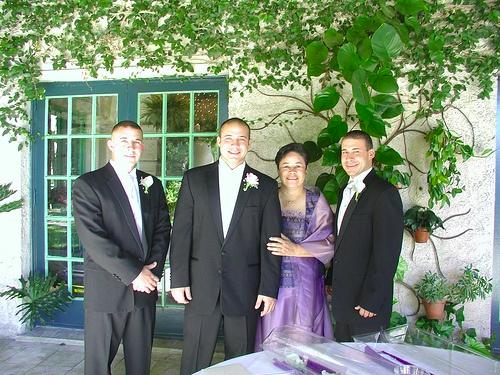
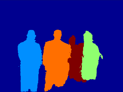
Here we visualize the feature representations built by our model at middle stages of its pipeline. To do so, we utilize the image in Fig. 5 (Left), which is one of the images from the validation Pascal VOC dataset that contained subjects.
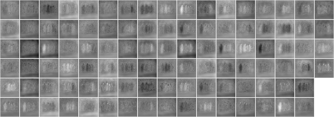
In Fig. 6 we visualize the features extracted in the output channels of the FCN stage of our model. Here we can see that different instances have different features at this level. Furthermore, some of the channels are somewhat sensitive to some body parts, particularly faces.
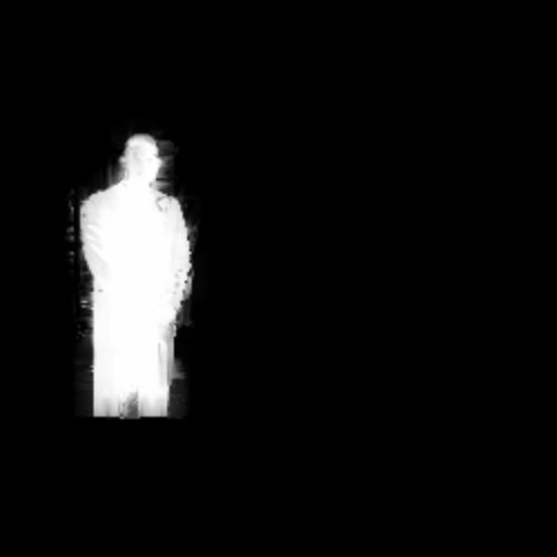
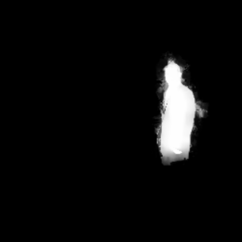
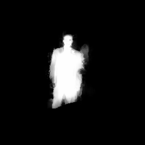
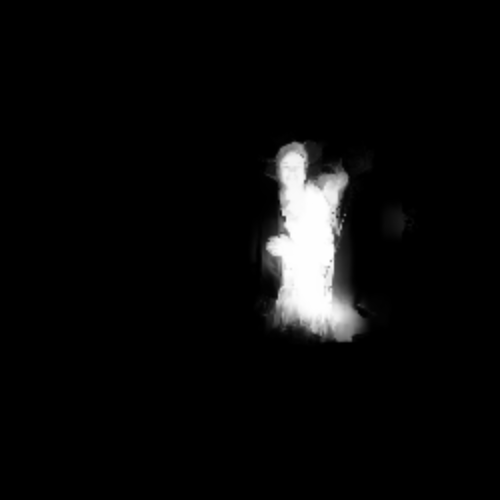
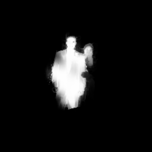
In Fig. 7 we see the state of the ConvLSTM, as well as the representation at two middle stages of the spatial inhibition module, as the model keeps producing segmentations of new instances. We also show the prediction and the confidence score.
In particular, the first row of Fig. 7 shows the absolute values across channels of the state . In the second row, we show the representation obtained after the convolution in the spatial inhibition module, which produces a 1-channel output. For the sake of clarity in the visualization, we have filtered out the pixels that have a negative value. We see that at this stage the representation is able to separate one object of interest, but it often contains other elements with lower intensity. In the third row, we show the representation obtained by the spatial inhibition module, just before the sigmoid transformation. Here we have also omitted the negative pixel values. We observe that the representation has successfully filtered out all pixels but the ones belonging to the object of interest. We also observed that the intensity values of the produced mask are not uniform. Finally, the following row shows the masks produced at the end of the pipeline (together with the confidence scores). The sigmoid operation allows the spatial inhibition module to produce pixel values that are saturated, that is, that are close to if they belong to the object of interest, or close to if they do not.
 |
 |
 |
 |
 |
|
 |
 |
 |
 |
 |
|
 |
 |
 |
 |
 |
|
 |
 |
 |
 |
 |
|
Appendix 0.B Diagram of ConvLSTM
Here we provide a diagram illustrating the recurrent update equations of the ConvLSTM (eq. 1).
Appendix 0.C Qualitative Results on Multiple Person Segmentation
In the following, we show some results produced by our model on multiple person segmentation.
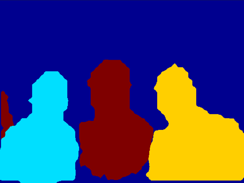
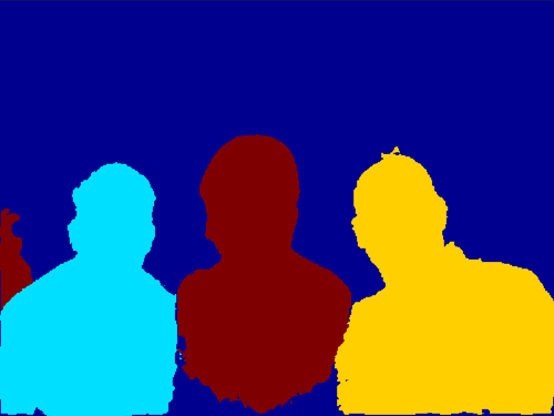
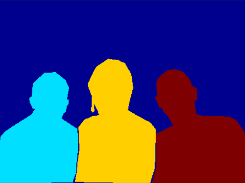
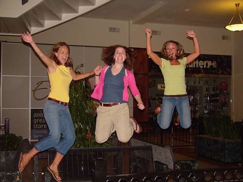
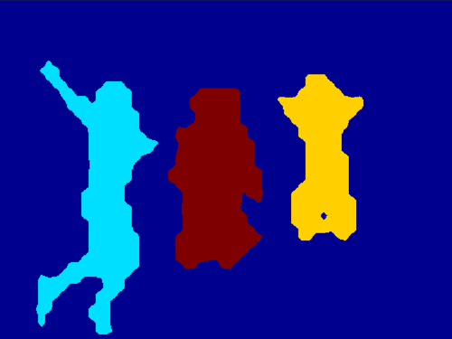
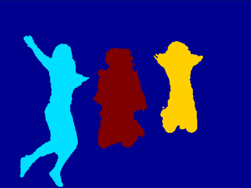
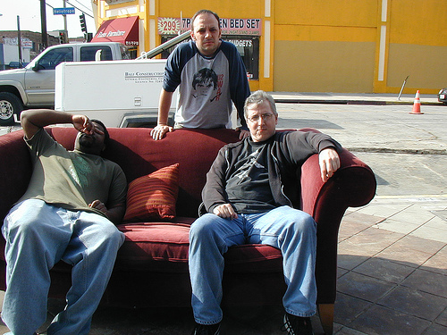
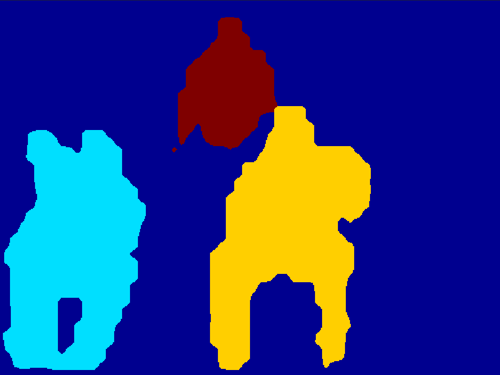
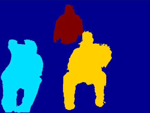
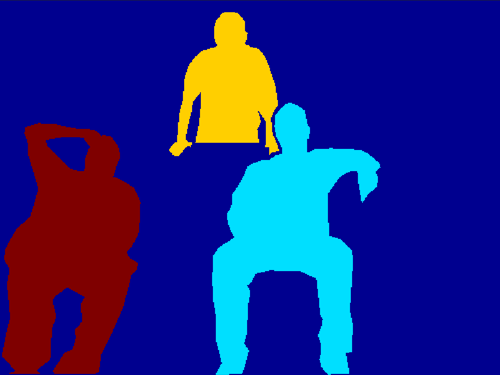
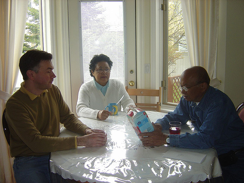
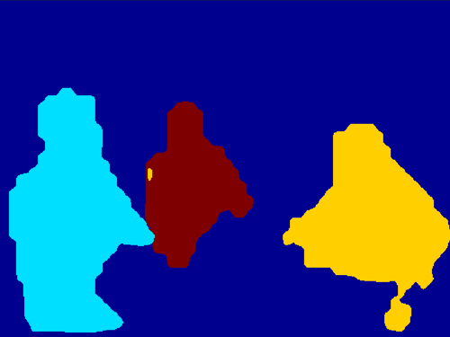
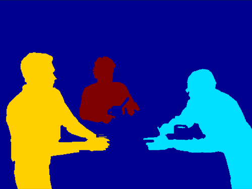
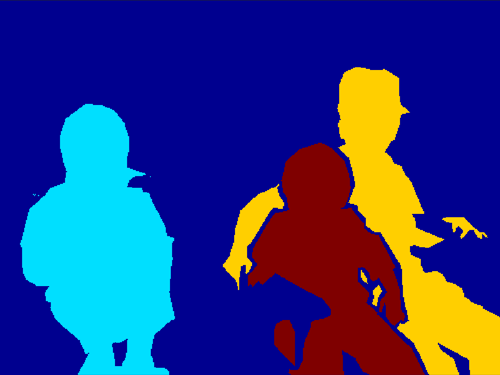
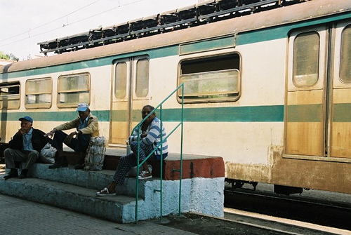
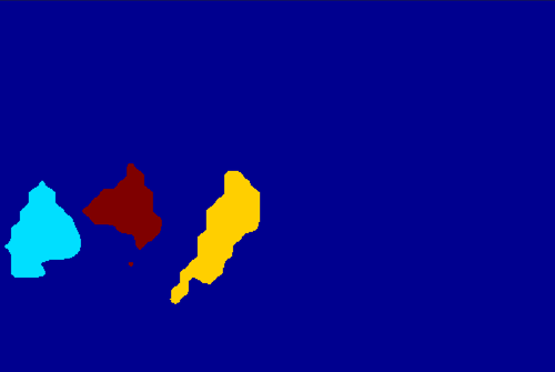
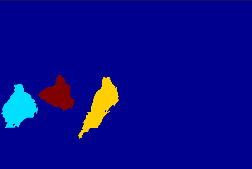
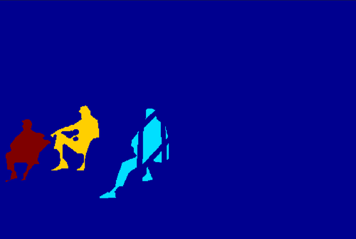
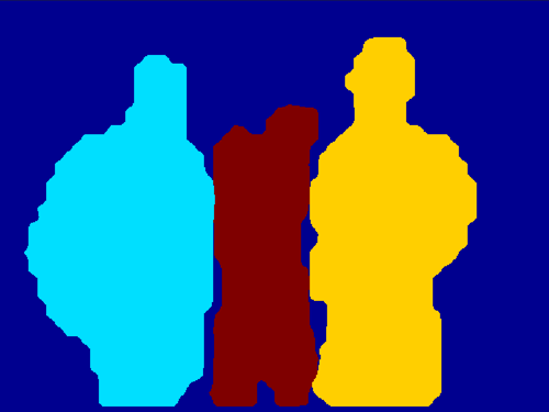
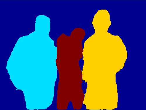
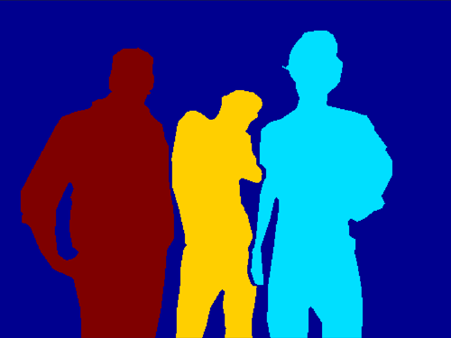
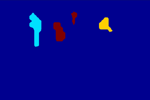
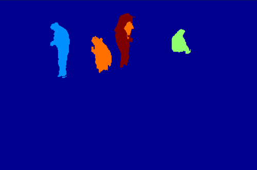
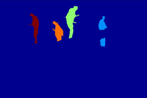
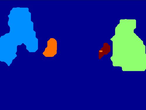
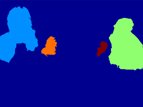
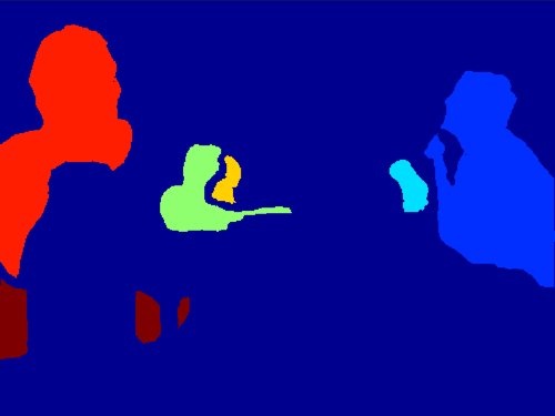
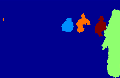
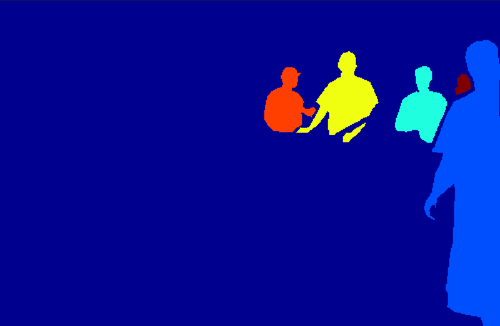
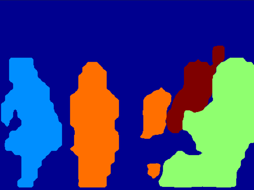
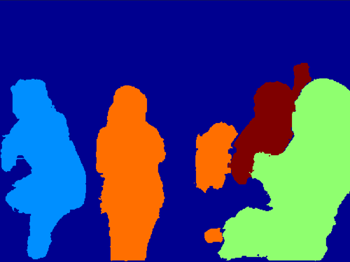
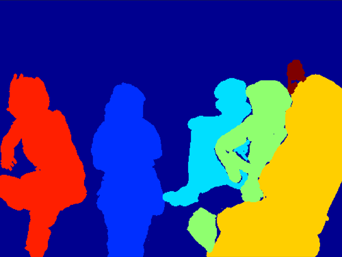
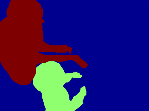
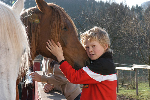
In Fig. 9, we show the outputs of our model (with and without CRF post-processing), with some input images containing subjects as ground truth. Note that the difference in colour (order) between ground truth instances and predictions is irrelevant. In these images the main errors are due to the difficulty to segment extremities (e.g. images in the second row).
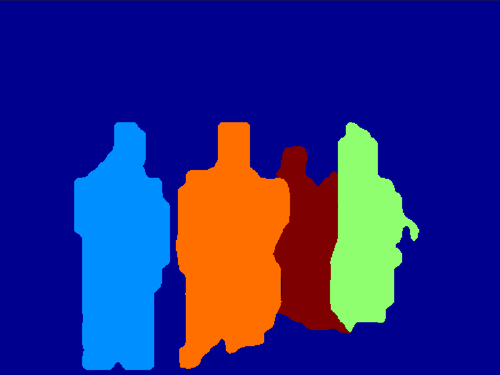
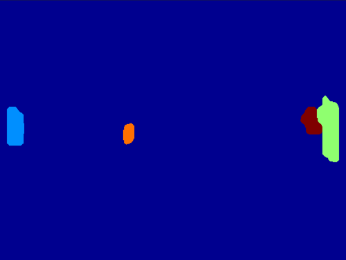
Similarly, in Fig. 10, we show the prediction of our model with images that contain or more subjects. In this case we see that our model struggles when segmenting more than instances (e.g. images in the sixth row), yet it is still able to provide good inferences, even in cases when the instances (subjects) appear far away (e.g. images in the second row).
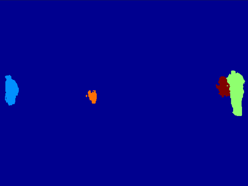
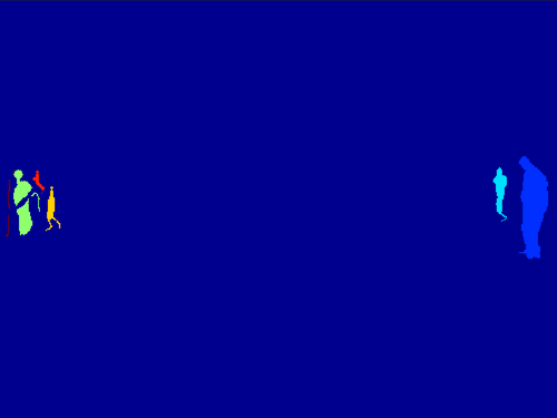
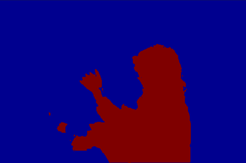
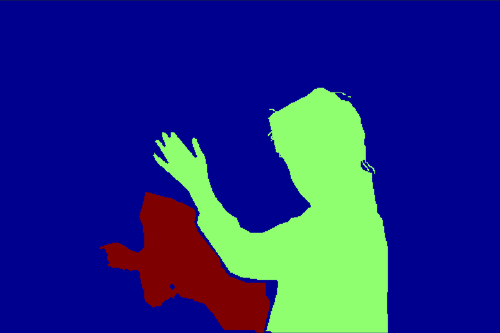
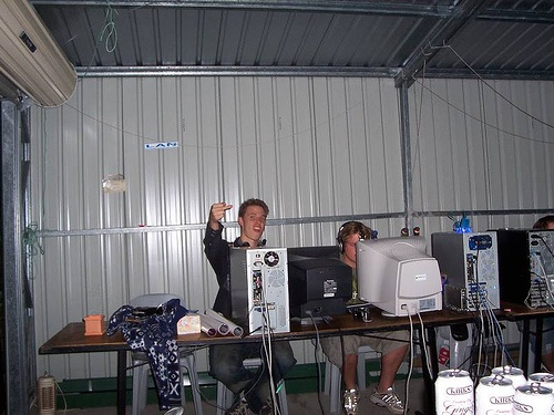
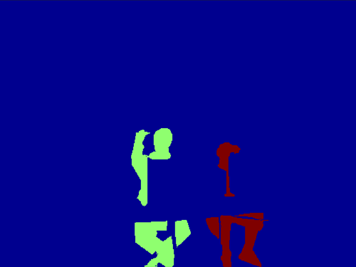
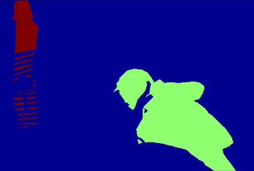
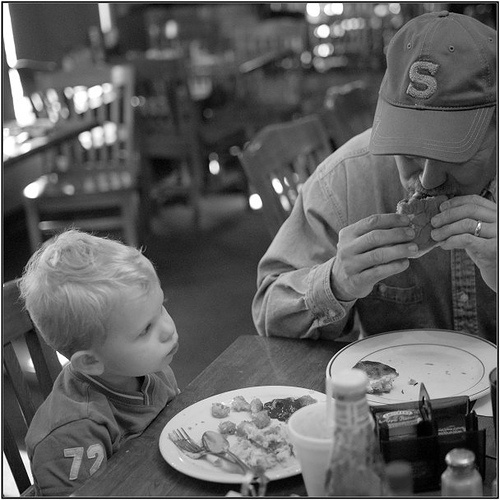
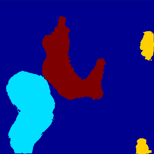
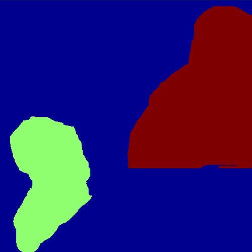
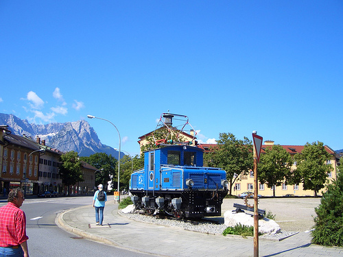
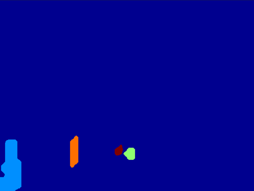
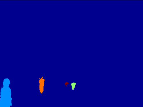
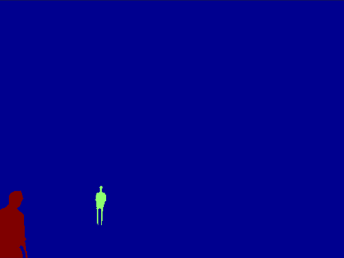
Finally, we have collected a set of failure cases. We have divided these in three classes which cover almost the entire range of failures we have seen. Firstly, our model might segment two instances as if they were only one. Examples of this are shown in Fig. 11. Secondly, our model sometimes misses an instance entirely, such as shown in the images in Fig. 12. Finally, we have seen that our model might hallucinate, that is, it might predict instances where there are none, see for example the images shown in Fig. 13.
| Input | RIS | RIS+CRF | Ground Truth |
|---|---|---|---|
 |
 |
 |
 |
 |
 |
 |
 |
 |
 |
 |
 |
 |
 |
 |
 |
 |
 |
 |
 |
 |
 |
 |
 |
 |
 |
 |
 |
| Input | RIS | RIS+CRF | Ground Truth |
|---|---|---|---|
 |
 |
 |
 |
 |
 |
 |
 |
 |
 |
 |
 |
 |
 |
 |
 |
 |
 |
 |
 |
 |
 |
 |
 |
 |
 |
 |
 |
| Input | RIS | RIS+CRF | Ground Truth |
|---|---|---|---|
 |
 |
 |
 |
 |
 |
 |
 |
| Input | RIS | RIS+CRF | Ground Truth |
|---|---|---|---|
 |
 |
 |
 |
 |
 |
 |
 |
| Input | RIS | RIS+CRF | Ground Truth |
|---|---|---|---|
 |
 |
 |
 |
 |
 |
 |
 |
Appendix 0.D Implementation of the Loss Function
In Algorithm 1 we provide a detailed implementation of the forward and backward propagation of the loss function in eq. (5).
The function finds the best matching given the matrix of values as an input. The functions and are the derivative functions of and with respect to their second argument.