Non-uniform Discontinuous Galerkin
Filters via Shift and Scale

Abstract

Convolving the output of Discontinuous Galerkin (DG) computations with symmetric Smoothness-Increasing Accuracy-Conserving (SIAC) filters can improve both smoothness and accuracy. To extend convolution to the boundaries, several one-sided spline filters have recently been developed. We interpret these filters as instances of a general class of position-dependent spline filters that we abbreviate as PSIAC filters. These filters may have a non-uniform knot sequence and may leave out some B-splines of the sequence.

For general position-dependent filters, we prove that rational knot sequences result in rational filter coefficients. We derive symbolic expressions for prototype knot sequences, typically integer sequences that may include repeated entries and corresponding B-splines, some of which may be skipped. Filters for shifted or scaled knot sequences are easily derived from these prototype filters so that a single filter can be re-used in different locations and at different scales. Moreover, the convolution itself reduces to executing a single dot product making it more stable and efficient than the existing approaches based on numerical integration. The construction is demonstrated for several established and one new boundary filter.

1 Introduction

Since the output of Discrete Galerkin (DG) computations often captures higher order moments of the true solution [ML78], postprocessing DG output by convolution can improve both smoothness and accuracy [BS77, CLSS03]. In the interior of the domain of computation, symmetric smoothness increasing accuracy conserving (SIAC) filters have been demonstrated to provide optimal accuracy [CLSS03]. However the symmetric footprint precludes using these filters near boundaries of the computational domain.

To address this problem Ryan and Shu [RS03] pioneered the use of one-sided spline filters. The Ryan-Shu filters improve the $L^{2}$ error, but not necessarily the point-wise errors. In fact, the filters are observed to increase the pointwise error near the boundary, motivating the design of the SRV filter [vSRV11], a filter kernel of increased support. Due to near-singular calculations, a stable numerical derivation of the SRV filter requires quadruple precision. Indeed, the coefficients of the boundary filters [RS03, vSRV11, MRK12, RLKV15, MRK15] are computed by inverting a matrix whose entries are computed by Gaussian quadrature; and, as pointed out in [RLKV15], SRV filter matrices are close to singular. [RLKV15] therefore introduced the RLKV filter, that augments the filter of [RS03] by a single additional B-spline. This improves stability and retains the support-size. However, RLKV filter errors on canonical test problems are higher than those of symmetric filters and they have sub-optimal $L^{2}$ and $L^{\infty}$ superconvergence rates [RLKV15], as well as poorer derivative approximation [LRKV16] than SRV filters. Consequently, SRV filters merit attention if their stablity can be improved.

The contribution of this paper is to reinterpret the published one-sided filters in the framework of position-dependent spline filters with general knot sequences [Pet15] (that were inspired by the partial symbolic expression of coefficients for uniform knot sequences in [MRK15]). This reinterpretation allows expressing and pre-solving them in sympbolic form, preempting instability so these filters can reach their full potential. Specifically, this paper

• proves general properties of SIAC filters, when their knots are shifted or scaled;

• uses the properties to express the kernels in a factored, semi-explicit form that becomes explicit for given knot patterns and yields rational coefficients for rational knot sequences;

• characterizes a class of position-dependent SIAC filters, short PSIAC filters, based on splines with general knot sequences; the coefficients of PSIAC filters are polynomial expressions in the position;

• shows that SRV and RLKV [RS03, vSRV11, MRK12, RLKV15, MRK15] are PSIAC filters; and

• illustrates the general framework by comparing the established numerical approach with the new symbolic filter derivation and by adding a new effective, stably-computed filter of lower degree than SRV or RLKV.

(a) DG output error	(b) SRV numerical approach	(c) SRV symbolic approach
	(b’) Left zoom of (b)	(c’) Left zoom of (c)

Figure 1: (a) Point-wise error of the $L^{2}$-projection of $u(x,0)=\frac{7}{10}\sin(\pi\sqrt{\frac{10}{7}}x)$ (interpreted as a DG approximation at time $\tau=0$) onto the space of piecewise cubic Bernstein-Bézier polynomials. The graphs in each figure correspond, from top to bottom, to refined intervals separated by $m=20,40,80$ break points. (b,c) Point-wise error after double precision convolution with the filter of [vSRV11] computed (b,b’) based on the numerical approach vs. (c,c’) as PSIAC filter using the symbolic approach. The vertical dotted lines separate the boundary region where position-dependent one-sided filters are applied from the interior where symmetric filters are applied.

The new characterization allows, in standard double precision, to replace the current three-step numerical approach of approximate computation of the matrix, its inversion and application to the data by Gauss quadrature, by a single-step symbolic approach derived in Theorem 4.1. Fig. 1 contrasts, for standard double precision, the noisy error of numerical SRV filtering with the error of the new symbolic formulation.

Not only is the symbolic approach more stable, but

• scaled and shifted version of the filter are easily obtained from one symbolic prototype filter;

• computation is more efficient: filtering the DG output reduces to a single dot product of two vectors of small size;

• stabilizes and simplifies computing approximate derivatives of the filtered DG output [RSA05] (see also [Tho77, RC09, LRKV16]) to differentiating the polynomial representation of the filtered output; and

• proves the smoothness of the so-filtered DG output to be $C^{\infty}$.

The last point is of interest since [RS03, vSRV11] observed and conjectured that the smoothness of the filtered DG computation is the same as the smoothness in the domain interior where the symmetric filter applied. Not only does this conjecture hold true, but Theorem 4.1 implies that the smoothness is $C^{\infty}$.

Organization.

Section 2 introduces the canonical test equation, B-splines, convolution, and a generalization of the formula of [Pet15] for convolution with splines based on arbitrary knot sequences. Section 3 reformulates the generalized convolution formula and derives the convolution coefficients when the knot sequence is a scaled or shifted copy of a prototype sequence. Section 4, in particular Theorem 4.1, summarizes the resulting efficient convolution with PSIAC filters based on scaled and shifted copies of a prototype sequence. Section 5 shows that SRV and RLKV are PSIAC filters and advertises their true potential by comparing their computation using the numerical approach to using the more stable symbolic approach. To illustrate the generality of the setup, a new multiple-knot linear filter is added to the picture.

2 Background

Here we establish the notation, distinguishing between filters and DG output, explain the canonical test problem, the DG method, B-splines and reproducing filters and we review one-sided and position-dependent SIAC filters in the literature.

2.1 Notation

Here and in the following, we abbreviate the sequences

$$i:j\,\, :=\,\,\begin{cases}(i,i+1,\ldots,j-1,j),\text{if }i\leq j,\\ (i,i-1,\ldots,j+1,j),\text{if }i>j,\end{cases}\quad s_{i:j}:=(s_{i},\ldots,s_{j}).$$

We denote by $f\ast g$ the convolution of a function $f$ with a function $g$, i.e.

$$(f\ast g)(x):=\int_{\mathbb{R}}f(t)\,g(x-t)\,\mathrm{d}t=(g\ast f)(x),$$

for every $x$ where the integral exists and we use the terms filter, filter kernel and kernel interchangeably, even though, strictly speaking, filtering means convolving a function with a kernel. We reserve the following symbols:

The notation is illustrated by the following example.

Example 2.1.

Consider a degree-one spline filter, i.e. $k=1$, defined over the knot sequence $\mathbf{t}:=0:6$ and associated with the index set $\scalebox{0.7}{$\mathcal{J}$}:=\{0,3,4\}$. That is, the two B-splines defined over the knot squences $1:3$ and $2:4$ are omitted, $n=6$, $r=2$ and ${j_{r}}=4$. A linear ($d=1$) DG output on 200 uniform segments of the interval $[-1..1]$ implies $m=200$, $h=\frac{1}{100}$ and $s_{0:m}=-100:100$.

2.2 The canonical test problem, the Discontinuous Galerkin method and B-splines

To demonstrate the performance of the filters on a concrete example, [RS03] used the following univariate hyperbolic partial differential wave equation:

$$\frac{du}{d\tau}+\frac{d}{dx}\Big{(}\kappa(x,\tau)\,u\Big{)} =\rho(x,\tau), x\in(a,b),\tau\in(0,\widetilde{\tau})$$ (1)

$$u(x,0) =u_{0}(x), x\in[a,b]$$

subject to periodic boundary conditions, $u(a,\tau)=u(b,\tau)$, or Dirichlet boundary conditions $u(e,\tau)=u_{0}(\tau)$ where, depending on the sign of $\kappa(x,\tau)$, $e$ is either $a$ or $b$. Subsequent work [RS03, vSRV11, RLKV15] adopted the same differential equation to test their new one-sided filters and to compare to the earlier work. Eq. (1) is therefore considered the canonical test problem. We note, however, that SIAC filters apply more widely, for example to FEM and elliptic equations [BS77].

In the DG method, the domain $[a..b]$ is partitioned into intervals by a sequence $hs_{0:m}$ of break points $a=:hs_{0},\ldots,hs_{m}:=b$. Assuming that the sequence is rational, introducing $h$ will allow us later to consider the prototype sequence $s_{0:m}$ of integers. The DG method approximates the time-dependent solution to Eq. (1) by

$$u(x,\tau):=\sum_{i=0}^{m}\,u_{i}(\tau)\,\phi_{i}(x\,;\,hs_{0:m}),$$ (2)

where the scalar-valued functions $\phi_{i}(.\,;\,hs_{0:m})$, $0\leq i\leq m$, are linearly independent and satisfy the scaling relations

$$\phi_{i}(hx\,;\,hs_{0:m})=\phi_{i}(x\,;\,s_{0:m}).$$ (3)

Examples of functions $\phi_{i}$ are non-uniform B-splines [dB05], Chebysev polynomials and Lagrange polynomials. Relation (3) is typically used for refinement in FEM, DG or Iso-geometric PDE solvers.

Setting $v(x):=\phi_{j}(x\,;\,hs_{0:m})$, the weak form of Eq. (1) for $j=0,1,\ldots,m$,

$$\int_{a}^{b}\big{(}\frac{du}{d\tau}\,v-\kappa(x,\tau)u\,\frac{dv}{dx}\big{)}\,\mathrm{d}x=\int_{a}^{b}\rho(x,\tau)\,v\,\mathrm{d}x-\Big{(}\kappa(x,\tau)u(x,\tau)v(x)\Big{)}\Big{|}_{x=a}^{x=b},$$ (4)

forms a system of ordinary differential equations with the coefficients $u_{i}(\tau)$, $0\leq i\leq m$, as unknowns.

The goal of SIAC filtering is to smooth $u(x,\tau)$ in $x$ by convolution in $x$ with a linear combination of B-splines. Typically filtering is applied after the last time step when $\tau=\widetilde{\tau}$. Following [Pet15], we characterize B-splines in terms of divided differences [CS66]. For a sufficiently smooth univariate real-valued function $g$ with $k$th derivative $g^{(k)}$, divided differences are defined by

$$\mathord{\kern 4.29993pt\vrule width=0.6pt,height=5.6pt,depth=-0.28pt\kern-4.29993pt\Delta}(t_{i})g :=g(t_{i}),\hskip 108.405pt\text{ and for }j>i$$

$$\mathord{\kern 4.29993pt\vrule width=0.6pt,height=5.6pt,depth=-0.28pt\kern-4.29993pt\Delta}(t_{i:j})g :=\begin{cases}(\mathord{\kern 4.29993pt\vrule width=0.6pt,height=5.6pt,depth=-0.28pt\kern-4.29993pt\Delta}(t_{i+1:j})g-\mathord{\kern 4.29993pt\vrule width=0.6pt,height=5.6pt,depth=-0.28pt\kern-4.29993pt\Delta}(t_{i:j-1})g)/(t_{j}-t_{i}),&\text{ if }t_{i}\neq t_{j},\\ \frac{1}{(j-i)!}\,g^{(j-i)}(t_{i}),&\text{ if }t_{i}=t_{j}.\end{cases}$$ (5)

If $t_{i:j}$ is a non-decreasing sequence, we call its elements $t_{\ell}$ knots and the classical definition of the B-spline of degree $k$ with knot sequence $t_{i:j},\,j:=i+k+1$ is

$$B(x|t_{i:j}) :=(t_{j}-t_{i})\ \mathord{\kern 4.29993pt\vrule width=0.6pt,height=5.6pt,depth=-0.28pt\kern-4.29993pt\Delta}(t_{i:j})(\max\{(\cdot-x),0\})^{k}.$$ (6)

Here $\mathord{\kern 4.29993pt\vrule width=0.6pt,height=5.6pt,depth=-0.28pt\kern-4.29993pt\Delta}(t_{i:j})$ acts on the function $g:t\to(\max\{(t-x),0\})^{k}$ for a given $x\in\mathbb{R}$. Consequently, a B-spline is a non-negative piecewise polynomial function in $x$ with support on the interval $[t_{i}..t_{j})$. If $\nu$ is the multiplicity of the number $t_{\ell}$ in the sequence $t_{i:j}$, then $B(x|t_{i:j})$ is at least $k-\nu$ times continuously differentiable at $t_{\ell}$. This definition of $B(t\,|\,t_{i:i+k+1})$ agrees, after scaling, with the definition $N(t\,|\,t_{i:i+k+1})$ of the B-spline by recurrence [dB02]:

$$N(t\,|\,t_{i:i+k+1})=\frac{t_{i+k+1}-t_{i}}{k+1}\,B(t\,|\,t_{i:i+k+1}).$$ (7)

2.3 SIAC filter kernel coefficients

A piecewise polynomial $f:\mathbb{R}\to\mathbb{R}$ is said to be a SIAC spline kernel of reproduction degree $r$ if convolution of $f$ with monomials reproduces the monomials up to degree $r$, i.e., if

$$(f\ast(\cdot)^{\delta})(x)=x^{\delta},\qquad\delta=0..r.$$ (8)

Mirzargar et al. [MRK15] derived semi-explicit formulas when the filter has uniform knots while [Pet15] gives semi-explicit formulas for the coefficients of spline kernels over general knot sequences. The following definition further generalizes these formulas by allowing to skip some B-splines when constructing the kernel.

Definition 2.1 (SIAC spline filter kernel).

Let $\scalebox{0.7}{$\mathcal{J}$}:=(0,\ldots,{j_{r}})$ be a sequence of strictly increasing integers between $0$ and ${j_{r}}$. A SIAC spline kernel of degree $k$ and reproduction degree $r$ with index sequence $\mathcal{J}$ and knot sequence $t_{0:n}$ is a spline

$$f(x):=\sum_{j\in\scalebox{0.7}{$\mathcal{J}$}}f_{j}B(x|t_{j:j+k+1}),$$

of degree $k$ with coefficients $f_{j}$ chosen so that

$$\Bigl{(}\sum_{j\in\scalebox{0.7}{$\mathcal{J}$}}f_{j}B(\cdot|t_{j:j+k+1})\ast(-\cdot)^{\delta}\Bigr{)}(x)=(-x)^{\delta},\qquad\delta=0,\ldots,r.$$ (8’)

When $\scalebox{0.7}{$\mathcal{J}$}\,=\,0:r$ then Definition 2.1 replicates the definition of [Pet15].

Lemma 2.1 (SIAC coefficients).

The vector $\mathbf{f}:=[f_{0},\ldots,f_{r}]^{\mathtt{t}}\in\mathbb{R}^{r+1}$ of B-spline coefficients of the SIAC filter with index sequence $\scalebox{0.7}{$\mathcal{J}$}:=(0,\ldots,{j_{r}})$ and knot sequence $\mathbf{t}:=t_{0:n}$ is

$$\mathbf{f}:=\text{first column of }M_{0,\mathbf{t},\scalebox{0.7}{$\mathcal{J}$}}^{-1},\qquad M_{0,\mathbf{t},\scalebox{0.7}{$\mathcal{J}$}}:=\left[\begin{matrix}\mathord{\kern 4.29993pt\vrule width=0.6pt,height=5.6pt,depth=-0.28pt\kern-4.29993pt\Delta}{t_{j:j+k+1}}x^{k+1+\delta}\end{matrix}\right]_{\delta=0:r,\,j\in\scalebox{0.7}{$\mathcal{J}$}}.$$ (9)

Proof.

We prove invertibility of $M_{0,\mathbf{t},\scalebox{0.7}{$\mathcal{J}$}}$. The remaining claims of the lemma then follow as in [Pet15].

Let $\ell$ be a left null vector of $M_{0,\mathbf{t},\scalebox{0.7}{$\mathcal{J}$}}$, i.e. for all $j\in\scalebox{0.7}{$\mathcal{J}$}$, $\kappa:=k+1$ and $p(x):=x^{\kappa}\sum_{\delta}\ell_{\delta}x^{\delta}$

$$0=\mathord{\kern 4.29993pt\vrule width=0.6pt,height=5.6pt,depth=-0.28pt\kern-4.29993pt\Delta}{t_{j:j+\kappa}}\sum_{\delta=0}^{r}\ell_{\delta}x^{\kappa+\delta}=\mathord{\kern 4.29993pt\vrule width=0.6pt,height=5.6pt,depth=-0.28pt\kern-4.29993pt\Delta}{t_{j:j+\kappa}}x^{\kappa}\sum_{\delta=0}^{r}\ell_{\delta}x^{\delta}=\mathord{\kern 4.29993pt\vrule width=0.6pt,height=5.6pt,depth=-0.28pt\kern-4.29993pt\Delta}{t_{j:j+\kappa}}p(x).$$ (10)

Let $q$ be the interpolant of $p$ at $t_{j:j+\kappa+1}$, i.e. spanning two consecutive hence overlapping knot sequences. If knots repeat, $q$ is a Hermite interpolant. By Rolle’s theorem, the derivative $D(p-q)$, vanishes at a set of knots $t^{1}_{j:j+\kappa}$ interlaced with $t_{j:j+\kappa+1}$, i.e. $t_{i}\leq t^{1}_{i}\leq t_{i+1}$. The inequality is strict unless $t_{i}=t^{1}_{i}$ represents a multiple root. Then $Dq$ (Hermite) interpolates $Dp$ at $t^{1}_{j:j+\kappa}$ and by the relation between divided difference and derivatives,

$$\kappa\mathord{\kern 4.29993pt\vrule width=0.6pt,height=5.6pt,depth=-0.28pt\kern-4.29993pt\Delta}{t_{j:j+\kappa}}p=\mathord{\kern 4.29993pt\vrule width=0.6pt,height=5.6pt,depth=-0.28pt\kern-4.29993pt\Delta}{t^{1}_{j:j+\kappa-1}}Dp \text{ and }\kappa\mathord{\kern 4.29993pt\vrule width=0.6pt,height=5.6pt,depth=-0.28pt\kern-4.29993pt\Delta}{t_{j+1:j+\kappa+1}}p=\mathord{\kern 4.29993pt\vrule width=0.6pt,height=5.6pt,depth=-0.28pt\kern-4.29993pt\Delta}{t^{1}_{j+1:j+\kappa}}Dp.$$

Induction yields

$$\kappa!\mathord{\kern 4.29993pt\vrule width=0.6pt,height=5.6pt,depth=-0.28pt\kern-4.29993pt\Delta}{t_{j:j+\kappa}}p=2\mathord{\kern 4.29993pt\vrule width=0.6pt,height=5.6pt,depth=-0.28pt\kern-4.29993pt\Delta}{t^{\kappa-1}_{j:j+1}}D^{\kappa-1}p, \text{ and }\kappa!\mathord{\kern 4.29993pt\vrule width=0.6pt,height=5.6pt,depth=-0.28pt\kern-4.29993pt\Delta}{t_{j+1:j+\kappa+1}}p=2\mathord{\kern 4.29993pt\vrule width=0.6pt,height=5.6pt,depth=-0.28pt\kern-4.29993pt\Delta}{t^{\kappa-1}_{j+1:j+2}}D^{\kappa-1}p$$

$$\text{ and finally }\kappa!\mathord{\kern 4.29993pt\vrule width=0.6pt,height=5.6pt,depth=-0.28pt\kern-4.29993pt\Delta}{t_{j:j+\kappa}}p=D^{\kappa}p(t^{\kappa}_{j}),\ \text{ and }\kappa!\mathord{\kern 4.29993pt\vrule width=0.6pt,height=5.6pt,depth=-0.28pt\kern-4.29993pt\Delta}{t_{j+1:j+\kappa+1}}p=D^{\kappa}p(t^{\kappa}_{j+1})$$

for $t^{\kappa}_{j}\leq t^{\kappa}_{j+1}$. That is, the $\kappa$th divided difference of each sequence equals the $\kappa$th derivative at points $t^{\kappa}_{j}$ respectively $t^{\kappa}_{j+1}$; and the shift of the subsequence of knots from $t_{j:j+\kappa}$ to $t_{j+1:j+\kappa+1}$ implies that where $t^{\kappa}_{j+1}$ is either strictly to the right of $t^{\kappa}_{j}$ or $t^{\kappa}_{j}$ is a multiple root. Then (10) implies that $D^{\kappa}p$, a polynomial of degree at most $r$, has $r+1$ roots counting multiplicity, hence is the zero polynomial. Given the factor $t^{\kappa}$ of $p$, this can only hold if $\ell=0$, i.e. $M_{0,\mathbf{t},\scalebox{0.7}{$\mathcal{J}$}}$ has no non-trivial left null vector and, as a square matrix, $M_{0,\mathbf{t},\scalebox{0.7}{$\mathcal{J}$}}$ is invertible.

Since all sequences $t_{j:j+\kappa}$, $j\in\scalebox{0.7}{$\mathcal{J}$}$ can be obtained by repeated shifts to the right, the conclusion $\ell=0$ holds for $j\in\scalebox{0.7}{$\mathcal{J}$}$ and $M^{-1}_{0,\mathbf{t},\scalebox{0.7}{$\mathcal{J}$}}$ is well-defined. ∎

2.4 Review of Symmetric and Boundary SIAC filters

We split the DG data at any known discontinuities and treat the domains separately. Then convolution can be applied throughout a given closed interval $[a..b]$.

A SIAC spline kernel with knot sequence $t_{0:r+k+1}$ is symmetric (about the origin in $\mathbb{R}$) if $t_{\ell}+t_{r+k+1-\ell}=0$ for $\ell=0:\lceil(r+k+1)/2\rceil$. Convolution with a symmetric SIAC kernel of a function $g$ at $x$ then requires $g$ to be defined in a two-sided neighborhood of $x$. Near boundaries, Ryan and Shu [RS03] therefore suggested convolving the DG output with a one-sided kernel whose support is shifted to one side of the origin: for $x$ near the left domain endpoint $a$, the one-sided SIAC kernel is defined over $(x-a)+h\big{(}-(3d+1):0\big{)}$ where $d$ is the degree of the DG output. The Ryan-Shu $x$-position-dependent one-sided kernel yields optimal $L^{2}$-convergence, but its point-wise error near $a$ can be larger than that of the DG output.

In [vSRV11], Ryan et al. improved the one-sided kernel by increasing its monomial reproduction from degree $r=2d$ to degree $r=4d$. This one-sided kernel reduces the boundary error when $d=1$ but the kernel support is increased by $2d$ additional knot intervals and numerical roundoff requires high precision calculations to determine the kernel’s coefficients. ([vSRV11] did not draw conclusions for degrees $d>1$.)

Ryan-Li-Kirby-Vuik [RLKV15] suggested an alternative position-dependent one-sided kernel that has the same support size as the symmetric kernel and its reproduction degree is only higher by one. The new idea is that the spline space defining the kernel is enriched by one B-spline. The new kernel computation is stable up to degree $d=4$ in double precision. When $d=1$ the RLKV kernel’s point-wise error on the canonical test problem is as low as that of the symmetric SIAC kernel that is applied in the interior. However, when $d>1$, the RLKV error is higher than that of the symmetric kernel.

In [RS03, vSRV11, MRK12, RLKV15] convolution with position-dependent one-sided kernels is computed as follows. For each domain position $x$,

• Calculate kernel coefficients:
  compute the entries of the position-dependent reproduction matrix $M$ by Gaussian quadrature; solve a corresponding linear system $M\mathbf{f}=\mathbf{p}$ for the kernel coefficients $\mathbf{f}$ to match the monomials to be reproduced, collected in the vector $\mathbf{p}$. As pointed out in [RLKV15], $M$ may be close to singular (for example, when $d\geq 3$ for the SRV kernels) so that higher numerical precision (e.g. quadruple precision) is required to assemble and solve the linear system.

• Convolve the kernel with the DG output by Gaussian quadrature.

Note that, unlike the (position-independent) classical symmetric SIAC filter, the position-dependent boundary kernel coefficients have to be determined afresh for each point $x$.

3 Coefficients of shifted and scaled filters

To calculate filters for DG output more efficiently and more stably, we reformulate Lemma 2.1 in multi-index notation:

$$t^{\boldsymbol{\omega}}_{0:n} :=t_{0}^{\omega_{0}}\ldots t_{n}^{\omega_{n}}\quad\text{and}\quad|t_{0:n}|:=\sum^{n}_{j=0}|t_{j}|$$

as follows.

Lemma 3.1 (SIAC reproduction matrix).

The matrix Eq. (9) has the alternative form

$$M:=M_{0,t_{0:n},\scalebox{0.7}{$\mathcal{J}$}} =\left[\begin{matrix}\sum\limits_{|{\boldsymbol{\omega}}|=\delta}t_{j:j+k+1}^{{\boldsymbol{\omega}}}\end{matrix}\right]_{\delta=0:r,\,j\in\scalebox{0.7}{$\mathcal{J}$}}.$$ (11)

Proof.

Applying Steffensen’s formula [dB05, Eq. (27)], the divided differences of monomials in (9) can be rewritten as (11). ∎

Denote the reproduction matrix associated with the shifted knot sequence $t_{j:j+k+1}+\xi,\,\xi\in\mathbb{R}$ as

$$M_{\xi}:=\left[\begin{matrix}\sum\limits_{|{\boldsymbol{\omega}}|=\delta}(t_{j:j+k+1}+\xi)^{{\boldsymbol{\omega}}}\end{matrix}\right]_{\delta=0:r,\,j\in\scalebox{0.7}{$\mathcal{J}$}}.$$ (12)

Since each entry $M_{\xi}(\delta,j)$ is a polynomial of degree $\delta$ in $\xi$, the determinant of $M_{\xi}$ is a polynomial of degree $r(r+1)/2$ in $\xi$. Using for example Cramer’s rule, the entries of $M^{-1}_{\xi}$ are rational functions in $\xi$ whose nominator and denominator are polynomials of degree $r(r+1)/2$ in $\xi$. Since the convolution coefficients are the entries of the first column of $M^{-1}_{\xi}$, it is remarkable, that we can show that the coefficients are not rational but polynomial and of degree $r$ rather than $r(r+1)/2$ in $\xi$.

To prove this claim, we employ the following technical result that generalizes a binomial indentity to multiple indices.

Lemma 3.2 (technical lemma).

We abbreviate $\binom{\mathbf{b}}{\mathbf{a}}:=\binom{b_{0}}{a_{0}}\ldots\binom{b_{k+1}}{a_{k+1}}$ and write $\mathbf{a}\leq\mathbf{b}$ to indicate that, for each $k\mathrm{th}$ component, $a_{k}\leq b_{k}$. Then for $\delta>|\mathbf{a}|$,

$$\sum_{\boldsymbol{\alpha}\geq\mathbf{a},\,|\boldsymbol{\alpha}|=\delta}\binom{\boldsymbol{\alpha}}{\mathbf{a}}=\binom{\delta+k+1}{|\mathbf{a}|+k+1}=\binom{\delta+k+1}{\delta-|\mathbf{a}|}.$$ (13)

Proof.

By the Maclaurin expansion: $\frac{1}{(1-x)^{k+1}}=\sum_{\ell=0}^{\infty}\binom{k+\ell}{k}x^{\ell}$, $|x|<1$, we see that

$$\frac{x^{k}}{(1-x)^{k+1}}=\sum_{\ell\geq k}\binom{\ell}{k}x^{\ell},\quad|x|<1.$$ (14)

Applying Eq. (14) to both sides of the identity

$$x^{k+1}\,\frac{x^{a_{0}}}{(1-x)^{a_{0}+1}}\cdots\frac{x^{a_{k+1}}}{(1-x)^{a_{k+1}+1}}=\frac{x^{|\mathbf{a}|+k+1}}{(1-x)^{|\mathbf{a}|+k+2}},$$ (15)

and dividing both sides by $x^{k+1}$, we see that

$$\sum_{\boldsymbol{\alpha}\geq\mathbf{a}}\binom{\boldsymbol{\alpha}}{\mathbf{a}}x^{|\boldsymbol{\alpha}|}=\sum_{\ell\geq|\mathbf{a}|+k+1}\binom{\ell}{|\mathbf{a}|+k+1}x^{\ell-k-1}.$$ (16)

Selecting the coefficients of $x^{\delta}$ from both sides of Eq. (16) yields Eq. (13). ∎

Lemma 3.3 (Reproduction matrix for shifted knots).

The matrices $M_{\xi}$ and $M:=M_{0,t_{0:n},\scalebox{0.7}{$\mathcal{J}$}}$ are related by

$$M_{\xi}=P_{k,r}(\xi)\,M:=\left[\begin{matrix}1\\ \binom{1+k+1}{1}\xi&1\\ \vdots&\vdots&\ddots\\ \binom{r+k+1}{r}\xi^{r}&\cdots&\binom{r+k+1}{1}\xi&1\end{matrix}\right]\,M.$$ (17)

(In (17), only non-zero entries are shown.) Note that $P_{k,r}(1)$ is the result of deleting the first $k+1$ rows and $k+1$ columns of the lower triangular Pascal matrix of order $r+k+1$.

Proof.

Abbreviating $\mathbf{t}_{j}:=t_{j:j+k+1}$, the entry $(\delta,j)$ of $M_{\xi}$ defined by Eq. (12) is

$$M_{\xi}(\delta,j) =\sum_{|\boldsymbol{\alpha}|=\delta}\sum_{\boldmath{0}\leq\boldsymbol{\ell}\leq\boldsymbol{\alpha}}\binom{\boldsymbol{\alpha}}{\boldsymbol{\ell}}\,\xi^{|\boldsymbol{\ell}|}\,\mathbf{t}_{j}^{\boldsymbol{\alpha}-\boldsymbol{\ell}}$$ (18)

$$=\sum_{|\boldsymbol{\alpha}|=\delta}\sum_{\beta=0}^{\delta}\xi^{\beta}\sum_{|\boldsymbol{\ell}|=\beta,\,\boldmath{0}\leq\boldsymbol{\ell}\leq\boldsymbol{\alpha}}\binom{\boldsymbol{\alpha}}{\boldsymbol{\ell}}\,\mathbf{t}_{j}^{\boldsymbol{\alpha}-\boldsymbol{\ell}}=\sum_{\beta=0}^{\delta}\xi^{\beta}\sum_{|\mathbf{a}|=\delta-\beta}\mathbf{t}_{j}^{\mathbf{a}}\sum_{|\boldsymbol{\alpha}|=\delta,\,\boldsymbol{\alpha}\geq\mathbf{a}}\binom{\boldsymbol{\alpha}}{\mathbf{a}}.$$

The last equality of Eq. (18) follows by substituting $\mathbf{a}=\boldsymbol{\alpha}-\boldsymbol{\ell}$. Applying Lemma 3.2 to Eq. (18) and noting that $|\mathbf{a}|=\delta-\beta$, we see that

$$M_{\xi}(\delta,j)=\sum_{\beta=0}^{\delta}\binom{\delta+k+1}{\beta}\xi^{\beta}M(\delta-\beta,j).$$ (19)

Eq. (19) is the expanded form of Eq. (17). ∎

Next we consider the effect of scaling knots, as might be done to refine a DG computation.

Lemma 3.4 (Reproduction matrix for scaled knots).

Let $\operatorname{diag}(\mathbf{v})$ denote the square matrix with diagonal $\mathbf{v}$ and zero otherwise. Then for $\mathbf{t}:=t_{0:n}$

$$M_{0,h\mathbf{t},\scalebox{0.7}{$\mathcal{J}$}}^{-1} =M_{0,\mathbf{t},\scalebox{0.7}{$\mathcal{J}$}}^{-1}\operatorname{diag}(h^{-(0:r)}), \text{ where }h^{-(0:r)}:=[1,h^{-1},\ldots,h^{-r}].$$ (20)

Proof.

By Lemma 3.1, multiplying the $(\delta+1)$-th row of $M_{0,\mathbf{t},\scalebox{0.7}{$\mathcal{J}$}}$ by $h^{\delta}$ yields $M_{0,h\mathbf{t},\scalebox{0.7}{$\mathcal{J}$}}$, $\delta=0,\ldots,r$ and hence

$$M_{0,h\mathbf{t},\scalebox{0.7}{$\mathcal{J}$}}=\operatorname{diag}([1,h,\ldots,h^{r}])\,M_{0,\mathbf{t},\scalebox{0.7}{$\mathcal{J}$}}$$

which is equivalent to (20). ∎

Alltogether, we obtain the following semi-explicit formula for the filter coefficients.

Theorem 3.1 (Scaled and shifted SIAC coefficients).

The SIAC filter coefficients $f_{\xi;\ell}$ associated with the knot sequence $h\mathbf{t}+\xi$ are polynomials of degree $r$ in $\xi$:

$$\mathbf{f}_{\xi}:=[f_{\xi,\ell}]_{\ell=0:r}=\ M_{0,\mathbf{t},\scalebox{0.7}{$\mathcal{J}$}}^{-1}\operatorname{diag}(\left[\begin{matrix}(-1)^{\ell}\,\binom{\ell+k+1}{\ell}\end{matrix}\right]_{\ell=0:r})\operatorname{diag}(h^{-(0:r)})\big{(}\xi^{0:r}\big{)}^{\mathtt{t}}.$$ (21)

Proof.

By Lemma 17 and Lemma 3.4, the matrix $M_{\xi}$ corresponding to the scaled and shifted knot sequence $h\mathbf{t}+\xi$ has the inverse

$$M_{\xi}^{-1}=M^{-1}_{0,\mathbf{t},\scalebox{0.7}{$\mathcal{J}$}}\operatorname{diag}(h^{-(0:r)})(P_{k,r}(\xi))^{-1}.$$ (22)

According to [ES04], $P_{k,r}(\xi)=(P_{k,r}(1))^{\xi}$ and hence $(P_{k,r}(\xi))^{-1}=P^{-\xi}_{k,r}(1)=P_{k,r}(-\xi)$. Since Theorem 2.1 requires only the first column of $M_{\xi}^{-1}$, we replace, in (22), $P_{k,r}(-\xi)$ by its first column and obtain

$$\mathbf{f}_{\xi}=M^{-1}_{0,\mathbf{t},\scalebox{0.7}{$\mathcal{J}$}}\,\operatorname{diag}(h^{-(0:r)})\,\operatorname{diag}(\left[\begin{matrix}(-1)^{\ell}\,\binom{\ell+k+1}{\ell}\end{matrix}\right]_{\ell=0:r})\,\big{(}\xi^{0:r}\big{)}^{\mathtt{t}}.$$ (23)

Eq. (21) follows, because the diagonal matrices commute. ∎

Compared to (23) formula (21) has the advantage that it groups together two matrices that can be pre-computed independent of $h$ and $\xi$.

The following corollary implies that the kernel coefficients $f_{\xi,\ell}$, can be computed stably, as scaled integers.

Corollary 3.1 (Rational SIAC filter coefficients $f_{\xi,\ell}$).

If the knots $t_{0:n}$ are rational, then the filter coefficients $f_{\xi,\ell}$ are polynomials in $\xi$ and $h$ with rational coefficients.

Proof.

Lemma 3.1 implies that the entries of $M$ are rational if the knots are rational. Since the determinant of a matrix with rational entries is rational, for example Cramer’s rule implies that the convolution coefficients are rational. ∎

4 Position-dependent (PSIAC) filtering

In this section, we first derive a general factored expression for the convolution of PSIAC filters with DG data. Then we specialize the setup to one-sided PSIAC filters when the DG breakpoint sequence is uniform.

4.1 Position-dependent (PSIAC) filters

When symmetric SIAC filtering increases the smoothness of the DG output, the result is in general a piecemeal function. One may expect the same of any one-sided kernel. However, this section proves that convolution with position-dependent PSIAC-filters yields a single polynomial piece over their interval of application. We start by defining position-dependent kernels.

Definition 4.1 (PSIAC kernel).

A PSIAC kernel at position $x$ has the form

$$f_{x}(s):=\sum_{j\in\scalebox{0.7}{$\mathcal{J}$}}\,f_{x;j}B(s\,|\,ht_{j:j+k+1}+x),\quad s\in h[t_{0},t_{n}]+x.$$ (24)

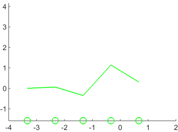
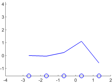
Figure 2: Position-dependent filtering at three locations $x$ (marked as a diamond) near the left endpoint (red diamond; denoted by $a$ in the text) of the piecwise linear DG output (note the small gaps between the segments). (Top) The resulting convolved values are marked by a star. (Bottom) The rightmost knot of the kernel is at location $x-a$.

Here we introduced the scaling $h$ in anticipation of using a prototype knot sequence, typically a subset of integers, to create one filter and then apply its shifts and its scaled version that can be cheaply computed as explained in the previous section. That is, the DG output will be convolved with a PSIAC kernel $f_{x-h\lambda}(s)$ of reproduction degree $r$, associated with an index sequence $\mathcal{J}$ and defined over the scaled and shifted knot sequence $ht_{0:n}+x-h\lambda$ where the constant $h\lambda$ adjusts to the left or right boundary. Substituting $x-h\lambda$ for $x$ in Eq. (24), changing variable from $s$ to $x-s$ and recalling that $n={j_{r}}+k+1$, we obtain an alternative spline representation of $f_{x-h\lambda}(s)$ with $x$-dependent coefficients $f_{{j_{r}}-j}:=f_{x-h\lambda;{j_{r}}-j}$ over the shifted and reversed knot sequence $h(\lambda-t_{n:0})$:

$$f_{x-h\lambda}(s)=\sum_{j\in\scalebox{0.7}{$\mathcal{J}$}}\,f_{{j_{r}}-j}\,B(x-s\,|\,h\lambda-ht_{n-j:{j_{r}}-j}),\quad s\in h[t_{0},t_{n}]+x-h\lambda.$$ (25)

Now consider the DG output $u(s,\tau)$ with break point sequence $s_{0:m}$ as in Eq. (2). Convolving $u(s,\tau)$ with $f_{x-h\lambda}(s)$ yields, after a change of variable $t:=x-s$, the filtered DG output

$$\big{(}u* f_{x-h\lambda}\big{)}(x)$$ (26)

$$=\sum_{j\in\scalebox{0.7}{$\mathcal{J}$}}f_{{j_{r}}-j}\,\int_{ht_{0}+x-h\lambda}^{ht_{n}+x-h\lambda}u(x-s,\tau)\,B(x-s\,|\,h\lambda-ht_{n-j:{j_{r}}-j})\,\mathrm{d}s$$

$$=\sum_{i\in\mathcal{I},\,j\in\scalebox{0.7}{$\mathcal{J}$}}u_{i}(\tau)\,f_{{j_{r}}-j}\,\int_{h\lambda-ht_{n}}^{h\lambda-ht_{0}}\phi_{i}(t\,;\,hs_{0:m})\,B(t\,|\,h\lambda-ht_{n-j:{j_{r}}-j})\,\mathrm{d}t.$$

We note that, in the last expression, the integral no longer depends on $x$. Rather, the coefficient $f_{{j_{r}}-j}:=f_{x-h\lambda;{j_{r}}-j}$ depends on $x$: by Theorem 21 $f_{{j_{r}}-j}$ is a polynomial in $x$. This yields the following factored representation of the convolution.

Theorem 4.1 (Efficient PSIAC filtering of DG output).

Let $f_{x}(s)$ be a PSIAC kernel of reproduction degree $r$ with index sequence $\scalebox{0.7}{$\mathcal{J}$}=(0,\ldots,{j_{r}})$ and knot sequence $ht_{0:n}+x-h\lambda$. Let $u(x,\tau):=\sum_{i=0}^{m}\,u_{i}(\tau)\,\phi_{i}(x\,;\,hs_{0:m}),$ $x\in[a,b]$ and $\tau\geq 0$, be the DG output. Let $\mathcal{I}$ be the set of indices of basis functions $\phi_{i}(.\,;\,hs_{0:m})$ with support overlapping $h[\lambda-t_{n},\lambda-t_{0}]$. Then the filtered DG approximation is a polynomial in $x$ of degree $r$:

$$\big{(}u*f_{x}\big{)}(x) =\mathbf{u}_{\mathcal{I}}\,Q_{\lambda}\,\operatorname{diag}(h^{-(0:r)})\,\big{(}(x-h\lambda)^{0:r}\big{)}^{\mathtt{t}}.$$ (27)

$$\mathbf{u}_{\mathcal{I}} :=[u_{i}(\tau)\big{]}_{i\in\mathcal{I}},$$

$$Q_{\lambda} :=G_{\lambda}\,A\,M^{-1}_{0,\mathbf{t},\scalebox{0.7}{$\mathcal{J}$}}\,\operatorname{diag}(\left[\begin{matrix}(-1)^{\ell}\,\binom{\ell+k+1}{\ell}\end{matrix}\right]_{\ell=0:r}),$$

$$G_{\lambda} :=\left[\int_{\lambda-t_{n}}^{\lambda-t_{0}}\,\phi_{i}(s\,;\,s_{0:m})\,B(s\,|\,\lambda-t_{n-j:{j_{r}}-j})\,\mathrm{d}s\right]_{i\in\mathcal{I},\,j\in\scalebox{0.7}{$\mathcal{J}$}},$$ (28)

and $A$ the reversal matrix (1 on the antidiagonal and zero else).

Proof.

Let $f_{r:0}:=f_{x-h\lambda;r:0}$ be the position-dependent coefficients of the parametrized kernel $f_{x-h\lambda}$ arranged in reverse order. We rewrite Eq. (26) as

$$\big{(}u* f_{x-h\lambda}\big{)}(x)=\mathbf{u}_{\mathcal{I}}\,G_{h\lambda}\,f_{r:0},$$ (29)

$$G_{h\lambda} :=\left[\int_{h(\lambda-t_{n})}^{h(\lambda-t_{0})}\,\phi_{i}(t\,;\,hs_{0:m})\,B(t\,|\,h\lambda-ht_{n-j:{j_{r}}-j})\,\mathrm{d}t\right]_{i\in\mathcal{I},\,j\in\scalebox{0.7}{$\mathcal{J}$}}.$$

Since $\phi(hs\,;\,h\cdot)=\phi(s\,;\,\cdot)$ by Eq. (3), $B(hs\,|\,h\lambda-ht_{n-j:{j_{r}}-j})=\frac{1}{h}B(s\,|\,\lambda-t_{n-j:{j_{r}}-j})$. Then the change of variable $s:=t/h$ yields

$$G_{h\lambda}(i,j) =\int_{\lambda-t_{n}}^{\lambda-t_{0}}\,\phi_{i}(hs\,;\,hs_{i:i+d+1})\,B(hs\,|\,h\lambda-ht_{n-j:{j_{r}}-j})\,h\,\mathrm{d}s=G_{\lambda}(i,j).$$

By Theorem 21

$$f_{r:0} =Af_{0:r}$$ (30)

$$=A\,M^{-1}_{0,t_{0:n},\scalebox{0.7}{$\mathcal{J}$}}\,\operatorname{diag}(\left[\begin{matrix}(-1)^{\ell}\,\binom{\ell+k+1}{\ell}\end{matrix}\right]_{\ell=0:r})\,\big{(}(x-h\lambda)^{0:r}\big{)}^{\mathtt{t}}.$$

Eq. (29) with Eq. (30) substituted equals Eq. (27). ∎

The factored representation implies that instead of recomputing the filter coefficients afresh for each point $x$ of the convolved output as in the established numerical approach, we simply compute the coefficients corresponding to one prototype knot sequence $\mathbf{t}$, scale by $h$ as needed and at runtime pre-multiply with the data and post-multiply with the vector of shifted monomials as stated in Eq. (27).

Increased multiplicity of an inner knot of the SIAC kernel reduces its smoothness, and this, in turn, reduces the smoothness of the filtered output. By contrast, Theorem 4.1 shows that when the PSIAC knots are shifted along evaluation points $x$ then PSIAC convolution yields a polyonomial, i.e. infinite smoothness regardless of the knot multiplicity. We may view position-dependent filtering as a form of polynomial approximation.

Additionally, the polynomial characterization directly provides a symbolic expression for the derivatives of the convolved DG output.

Corollary 4.1 (Derivatives of PSIAC-filtered DG output).

$$\frac{\mathrm{d}^{\ell}}{\mathrm{d}x^{\ell}}\big{(}u*f_{x}\big{)}(x)=\mathbf{u}_{\mathcal{I}}\,Q_{\lambda}\,\operatorname{diag}(h^{-(0:r)})\,\big{(}\frac{\mathrm{d}^{\ell}}{\mathrm{d}x^{\ell}}(x-h\lambda)^{0:r}\big{)}^{\mathtt{t}}.$$ (31)

The following Corollary shows that for rational DG break points and rational kernel knots, we can pre-compute and store the prototype matrix $Q_{\lambda}$ stably in terms of integer fractions.

Corollary 4.2 (Rational PSIAC convolution coefficients).

With the assumptions and notation of Theorem 4.1, if the basis functions $\phi_{i}(.\,;\,s_{0:m})$ are piecewise polynomials with rational coefficients, the shift $\lambda$ is rational and the sequences $t_{0:n}$ and $s_{0:m}$ are rational then the matrix $Q_{\lambda}$ has rational entries.

Proof.

By Lemma 3.1, the reproduction matrix $M^{-1}_{0,\mathbf{t},\scalebox{0.7}{$\mathcal{J}$}}$ has rational entries. Since the integral of a polynomial with rational coefficients over an interval with rational end points is rational, Eq. (28) implies that $G_{\lambda}$ also has rational entries. This implies that the entries of $Q_{\lambda}$ are rational. ∎

4.2 Application to filtering at boundaries

We now derive explicit forms of the matrix $G_{\lambda}$ of Theorem 4.1 when the DG break points $s_{0:m}$ are uniform and the PSIAC filters are one-sided. For one-sided filters, $\lambda$ is replaced by $\lambda_{L}$ and $\lambda_{R}$ for the left-sided and right-sided kernels respectively. Recalling that convolution reverses the direction of the filter kernel (cf. Fig. 2), it is natural to assume that the right-most knot of the left boundary kernel vanishes when evaluating at the left endpoint $x=a$, i.e. $(ht_{n}+x-h\lambda_{L})|_{x=a}=0$. Together with the analoguous assumption for right boundary kernels, this determines

$$\lambda_{L}=t_{n}+\frac{a}{h},\qquad\lambda_{R}=t_{0}+\frac{b}{h}.$$ (32)

Corollary 4.3 (PSIAC convolution coefficients for uniform DG knots).

Assume that the DG break point sequence $s_{0:m}$ is uniform, hence after scaling consists of consecutive integers. Without loss of generality, the DG output on each interval $[s_{i},s_{i+1}]$ is defined in terms of Bernstein-Bézier polynomials $B_{\ell}^{(i)}$, $\ell=0:d$, of degree $d$, i.e.

$$B_{\ell}^{(i)}(x):=\begin{cases}\binom{d}{\ell}(x-s_{i})^{\ell}(s_{i+1}-x)^{d-\ell}\quad&\text{if $x\in[s_{i},s_{i+1}]$}\\ 0\quad&\text{otherwise.}\end{cases}$$

Let $n_{0}$ be the smallest integer greater than or equal to $t_{n}-t_{0}$. Then, for $i=0:(n_{0}-1)$, $\ell=0:d$, and $j\in\scalebox{0.7}{$\mathcal{J}$}$

$$G_{\lambda_{L}}\big{(}(d+1)i+\ell,j\big{)} =\int_{i}^{i+1}B_{\ell}^{(i)}(t)\,B(t\,|\,t_{n}-t_{n-j:{j_{r}}-j)})\,\mathrm{d}t,$$ (33)

$$G_{\lambda_{R}}\big{(}(d+1)i+\ell,j\big{)} =\int_{n_{0}-i}^{n_{0}-i+1}B_{d-\ell}^{(n_{0}-i)}(t)\,B(t\,|\,t_{j:j+k+1}-t_{0})\,\mathrm{d}t.$$

Proof.

First we consider $G_{\lambda_{L}}$. In Eq. (28), we change to the variable $t=s-\lambda_{L}+t_{n}$. Abbreviating $\widehat{t}_{j}:=t_{n}-t_{n-j}$, since the B-splines are translation invariant, for $0\leq\widehat{t}_{j}=t_{n}-t_{n-j}\leq t_{n}-t_{0}\leq n_{0}$,

$$G_{\lambda_{L}}(i,j)=\int_{0}^{t_{n}-t_{0}}\,\phi_{i}(t\,;\,s_{0:m}-\lambda_{L}+t_{n})\,B(t\,|\,\widehat{t}_{j:j+k+1})\,\mathrm{d}t.$$ (34)

Since $s_{0}=\frac{a}{h}$, Eq. (32) implies that the first point of the sequence of translated DG break points $s_{0:m}-\lambda_{L}+t_{n}$ equals $0$, i.e., $s_{0}-\lambda_{L}+t_{n}=0$. Since the break points are consecutive integers starting from $0$ and $0\leq\widehat{t}_{j}\leq n_{0}$ the relevant DG break points are $0:n_{0}$. We re-index the basis functions $\phi_{i}(s\,;\,s_{0:m}-\lambda_{L}+t_{n})$ in terms of the Bernstein-Bézier basis functions $B_{\ell}^{(i)}$. Since $B_{\ell}^{(i)}$ are non-zero on any interval $[i,i+1]$, Eq. (33) for $G_{\lambda_{L}}$ follows from Eq. (34).

Now consider $G_{\lambda_{R}}$. The change of variable $t:=-(s-\lambda_{R}+t_{0})$ together with the translation invariance of B-splines imply that

$$G_{\lambda_{R}}(i,j) =\int_{0}^{t_{n}-t_{0}}\,\phi_{i}(-t\,;\,s_{0:m}-\lambda_{R}+t_{0})\,B(-t\,|\,t_{0}-t_{n-j:{j_{r}}-j})\,\mathrm{d}t.$$

$$=\int_{0}^{t_{n}-t_{0}}\,\phi_{m-i}(t\,;\,\lambda_{R}-t_{0}-s_{m:0})\,B(t\,|\,t_{j:j+k+1}-t_{0})\,\mathrm{d}t.$$ (35)

Because of Eq. (32) and $s_{m}=\frac{b}{h}$, $\lambda_{R}-t_{0}-s_{m}=0$. Eq. (33) is derived by re-indexing the basis functions $\phi_{m-i}$ as for the left boundary except that we have to count the functions $B_{\ell}^{(i)}$ backward from the last interval $[t_{n_{0}-1},t_{n_{0}}]$ to the first one $[t_{0},t_{1}]$ when $i$ and $j$ increase. ∎

The assumption that the DG output is represented in Bernstein-Bézier form, represents no restriction: the DG output can be represented in any piecewise polynomial form to arrive at similar formulas.

5 PSIAC kernels

In this section, we first restate the SRV and the RLKV filters as PSIAC filters and compare convolution using the numerical approach to using the symbolic approach. Second, to illustrate the generality of the setup, a new multiple-knot linear filter is defined and compared to the SRV and the RLKV filters.

5.1 An alternative view of the published boundary filters

We now recast several published boundary filters as special cases of PSIAC kernels defined over shifted knots in the sense of Theorem 4.1. The published filters considered in this section all chose $d=k$, i.e. the filter has the same degree as the DG output.

The boundary SIAC filters RS [RS03] and SRV [vSRV11] of reproduction degree $r$ are both defined over the following shifted knots:

$$\mu:=\frac{r+d+1}{2},\quad\lambda_{L,d}:=a+\mu,\quad\lambda_{R,d}:=b-\mu$$

$${\boldsymbol{t}}_{*,d}(x):=\Big{(}-\mu,-\mu+1,\ldots,\mu\Big{)}+x-\lambda_{*,d}.$$ (36)

Here $L$ or $R$ are substituted for $*$, we obtain the left-side and the right-side filters respectively. Both types of filter are associated with a consecutive index sequence $\mathcal{J}$ . However, the two kernels have different reproduction degrees: $r(\text{RS})=2d$ and $r(\text{RV})=4d$. The prototype knot sequences ${\boldsymbol{t}}_{*,d}(\lambda_{*,d})$ are chosen symmetrically supported about the origin.

In Proposition 5.1 below we denote as $\mathbf{b}_{k}$ the vectors of Bernstein-Bézier coefficients of the $d+1$ polynomial pieces of the uniform B-spline of degree $d$ defined over the knots $0:(d+1)$. For example,

$$d=1:\quad\left[\mathbf{b}_{0}\,\mathbf{b}_{1}\right]=\left[\begin{smallmatrix}0&1\\ 1&0\end{smallmatrix}\right]$$

$$d=2:\quad\left[\mathbf{b}_{0}\,\mathbf{b}_{1}\,\mathbf{b}_{2}\right]=\frac{1}{2}\left[\begin{smallmatrix}0&1&1\\ 0&2&0\\ 1&1&0\end{smallmatrix}\right]$$ (37)

$$d=3:\quad\left[\mathbf{b}_{0}\,\mathbf{b}_{1}\,\mathbf{b}_{2}\,\mathbf{b}_{3}\right]=\frac{1}{6}\left[\begin{smallmatrix}0&1&4&1\\ 0&2&4&0\\ 0&4&2&0\\ 1&4&1&0\end{smallmatrix}\right].$$

Proposition 5.1.

Let $\mathbf{b}_{k}$ denote the Bernstein-Bézier coefficients of polynomial pieces of a uniform B-spline of degree $d$ defined over the knots $0:(d+1)$ and $\mathcal{M}_{d}$ the matrix with entries $\mathcal{M}_{d}(\ell,j):=\frac{1}{2d+1}\binom{d}{\ell}\binom{d}{j}\binom{2d}{\ell+j}^{-1}$, $\ell,j=0:d$. Then

$$G_{\lambda_{L}}:=G_{\lambda_{L,d}}=\left[\begin{smallmatrix}\mathcal{M}_{d}\mathbf{b}_{0}&0&\cdots&0\\ \mathcal{M}_{d}\mathbf{b}_{1}&\mathcal{M}_{d}\mathbf{b}_{0}&\cdots&0\\ \vdots&\vdots&\cdots&\vdots\\ \mathcal{M}_{d}\mathbf{b}_{d}&\mathcal{M}_{d}\mathbf{b}_{d-1}&\cdots&0\\ 0&\mathcal{M}_{d}\mathbf{b}_{d}&\cdots&0\\ \vdots&\vdots&\cdots&\vdots\\ 0&0&\cdots&\mathcal{M}_{d}\mathbf{b}_{0}\\ \vdots&\vdots&\cdots&\vdots\\ 0&0&\cdots&\mathcal{M}_{d}\mathbf{b}_{d}\end{smallmatrix}\right]$$ (38)

and $G_{\lambda_{R}}$ is obtained from $G_{\lambda_{L}}$ by reversing the order of the columns and of the rows.

Proof.

Using the notation of Corollary 4.3, $n_{0}=n=r+d$, since $\widehat{t}_{0:n}=t_{n}-t_{n:0}=0..(r+d)$,

$$G_{\lambda_{L}}\big{(}(d+1)i+\ell,j\big{)}=\int_{i}^{i+1}B_{\ell}^{(i)}(t)\,B(t\,|\,j:j+d+1)\,\mathrm{d}t,$$ (39)

When $i$ and $\ell$ vary, Eq. (39) gives the $j$th column of $G_{\lambda_{L}}$. The support of $B(t\,|\,j:j+d+1)$ contains $d+1$ intervals $[j+\rho,j+\rho+1]$, $\rho=0:d$. When $[i,i+1]\equiv[j+\rho,j+\rho+1]$, i.e. when $i=j+\rho$, we can rewrite Eq. (39) as

$$\left[G_{\lambda_{L}}\big{(}(d+1)i+\ell,j\big{)}\right]_{\ell=0:d} =\int_{i}^{i+1}\left[B_{\ell}^{(i)}(t)\right]^{\mathtt{t}}_{\ell=0:d}\,\left[B_{j}^{(i)}(t)\right]_{j=0:d}\mathbf{b}_{\rho}\,\mathrm{d}t,$$ (40)

$$=\left[\int_{0}^{1}B_{\ell}^{(0)}(t)\,B_{j}^{(0)}(t)\,\mathrm{d}t\right]_{\ell=0:d,j=0:d}\mathbf{b}_{\rho}=\mathcal{M}_{d}\mathbf{b}_{\rho},$$

where

$$\mathcal{M}_{d}(\ell,j)=\binom{d}{\ell}\,\binom{d}{j}\,\binom{2d}{\ell+j}^{-1}\,\int_{0}^{1}\binom{2d}{\ell+j}x^{\ell+j}(1-x)^{2d-\ell-j}\,\mathrm{d}t.$$ (41)

Since the integral in Eq. (41) equals $\frac{1}{2d+1}$, we have derived the formula for $\mathcal{M}_{d}(\ell,j)$ in Eq. (38). The formula for $G_{\lambda_{L}}$ follows, because the entries of the $j$th column vanish when the two intervals $[i,i+1]$ and $[j+\rho,j+\rho+1]$ do not overlap.

The formula for $G_{\lambda_{R}}$ in Eq. (33) is that of $G_{\lambda_{L}}$ except that the B-splines appear in reverse order. Therefore, reversing the column order of $G_{\lambda_{L}}$ and then the row order of the result yields $G_{\lambda_{R}}$. ∎

The index sequence $\mathcal{J}$ of the boundary kernel RLKV is non-consecutive. The left and right kernels are of degree $2d+1$ and are defined over the following shifted knots

$${\boldsymbol{t}}_{L,d}(x) :=\Big{(}-\mu,\ldots,\mu-1,\underbrace{\mu,\ldots,\mu}_{\text{$d+1$ times}}\Big{)}+x-\lambda_{L,d},$$ (42)

$$\scalebox{0.7}{$\mathcal{J}$}_{L} :=\{1:(2d+1),3d+1\};$$

$${\boldsymbol{t}}_{R,d}(x) :=\Big{(}\underbrace{-\mu,\ldots,-\mu}_{\text{$d+1$ times}},-\mu+1,\ldots,\mu,\Big{)}+x-\lambda_{R,d},$$ (43)

$$\scalebox{0.7}{$\mathcal{J}$}_{R} :=\{1,d:(3d+1)\}.$$

The prototype knot sequence ${\boldsymbol{t}}_{L,d}(\lambda_{L,d})$ is chosen to have symmetric support about the origin.

Proposition 5.2.

Let $\mathcal{M}_{d}$ be defined as in Proposition 5.1 and let $\mathcal{M}_{d}^{(1)}$ denote its first column. Then

$$G_{\lambda_{L,d}}=\left[\begin{smallmatrix}(d+1)\mathcal{M}_{d}^{(1)}&\mathcal{M}_{d}\mathbf{b}_{0}&0&\cdots&0\\ 0&\mathcal{M}_{d}\mathbf{b}_{1}&\mathcal{M}_{d}\mathbf{b}_{0}&\cdots&0\\ \vdots&\vdots&\vdots&\cdots&\vdots\\ 0&\mathcal{M}_{d}\mathbf{b}_{d}&\mathcal{M}_{d}\mathbf{b}_{d-1}&\cdots&0\\ 0&0&\mathcal{M}_{d}\mathbf{b}_{d}&\cdots&0\\ \vdots&\vdots&\vdots&\cdots&\vdots\\ 0&0&0&\cdots&\mathcal{M}_{d}\mathbf{b}_{0}\\ \vdots&\vdots&\vdots&\cdots&\vdots\\ 0&0&0&\cdots&\mathcal{M}_{d}\mathbf{b}_{d}\end{smallmatrix}\right]$$ (44)

$G_{\lambda_{R}}$ is obtained from $G_{\lambda_{L}}$ by reversing the order of the columns and of the rows.

Proof.

The proof is the same as that of Proposition 5.1 except that the additional B-spline of the kernel contributes the first column of (44). ∎

5.2 A multiple-knot boundary PSIAC  kernel

Since their introduction in the seminal paper [RS03], boundary kernels have been given the same degree as the symmetric kernel [RLKV15] – perhaps to guarantee the same smoothness near the boundary as in domain interior. Indeed, the authors of [vSRV11] numerically observed and predicted that SRV-filtered DG outputs would be as smooth as the SRV kernel. Theorem 4.1 implies not only that a PSIAC kernel need not have the same degree as the symmetric kernel, but confirms smoothness of the output beyond the conjecture: it shows that PSIAC kernels may have multiple knots without reducing the the infinity smoothness of the filtered DG output.

We define a new multiple-knot left-sided kernel $f_{L}$ and a right-sided kernel $f_{R}$ each of degree $k=1$ (hence double-knot filters) respectively over the knot sequences

$$\boldsymbol{t}_{L} :=x-\lambda_{L}+\big{(}-\mu,\ldots,\mu-3,\mu-2,\mu-1,\mu-1,\mu,\mu\big{)},\ \mu:=\frac{3d+1}{2},$$

$$\boldsymbol{t}_{R} :=x-\lambda_{R}+\big{(}-\mu,-\mu,-\mu+1,-\mu+1,-\mu+2,-\mu+3\ldots,\mu\big{)}.$$ (45)

Since the degree of the kernels is $1$, their reproduction degree is $3d+2$ even though they have the same support size as the symmetric SIAC kernel that one might apply in the interior of the $DG$ domain. The two double-knots increase the reproduction degree but not the support.

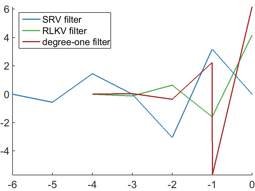
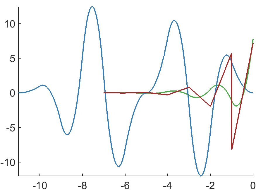
(a) kernels for $d=1$	(b) kernels for $d=2$
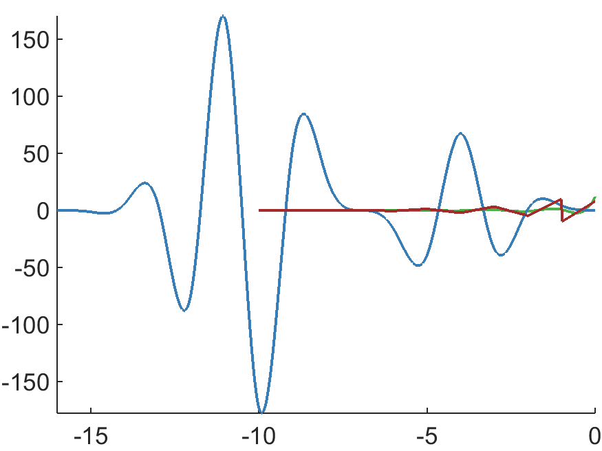
(c) kernels for $d=3$	(c’) right zoom of (c)

Figure 3: Graphs of the three kernels defined at the left boundary $x=a$. Note that the degree of [vSRV11] and [RLKV15] increases with $d$ while the degree of the multiple-knot kernel stays linear.

5.3 Examples

Fig. 3 graphs instances of the [vSRV11], [RLKV15] and of the new multiple-knot kernel of degree-one. With the help of the following two examples we numerically verify the symbolic expression (27). We demonstrate improved stability of the symbolic approach over the numerical approach and we illustrate a possible use of a kernel of degree $k\neq d$ (we will choose $k=1<d$) and illustrate a possible use of inner knots with higher multiplicity. Both examples are special cases of the canonical Eq. (1) with

$$\kappa(x,\tau)\equiv 1,\quad\rho(x,\tau)\equiv 0,\quad 0\leq\tau\leq\widetilde{\tau}.$$ (46)

Example 1 Consider Eq. (1) with specialization (46), Dirichlet boundary conditions and $\widetilde{\tau}:=\frac{1}{16}$. The exact solution is $u(x,\widetilde{\tau})=\frac{7}{10}\sin(\pi\sqrt{\frac{10}{7}}(x-\widetilde{\tau}))$.

Example 2 Consider Eq. (1) with specialization (46), periodic boundary conditions and $\widetilde{\tau}:=1$, i.e. after a sequence of time steps. The exact solution is $u(x,\widetilde{\tau})=\sin(2\pi(x-\widetilde{\tau}))$.

(a) Example 1 DG $d=2$ output error

(b) [vSRV11] numerical

(c) [vSRV11] symbolic

(d) Left zoom of 4(b)

(e) Left zoom of 4(c)

(f) [RLKV15]

(g) new multiple-knot filter

Figure 4: Point-wise errors of DG approximations of Example 1 when $d=2$. The three graphs in each subfigure correspond, from top to bottom, (red, blue, green) to $m=20,40$ and $80$ DG break points.

(a) Example 2 DG $d=3$ output error

(b) [vSRV11] numerical

(c) [vSRV11] symbolic

(d) Left zoom of 5(b)

(e) Left zoom of 5(c)

(f) [RLKV15]

(g) new multiple-knot filter

Figure 5: Point-wise errors of DG approximations of Example 2 when $d=3$. The three graphs in each subfigure correspond, from top to bottom, (red, blue, green) to $m=20,40$ and $80$ DG break points.

We used upwind numerical flux [HW07] and solved the resulting ordinary differential equations with the help of a standard fourth-order four stage explicit Runge-Kutta method (ERK) [HW07, Section 3.4]. Figures 4 and 5 show the error of the DG approximations of Example 1 and Example 2, respectively, when using different post-filters.

For [vSRV11], the numerical approach introduces high oscillations in the point-wise errors near the boundaries for both example problems. The increase of the oscillations with decreasing mesh size is the result of near-singular matrices: when $m=80$ and $d=3$, the matrices $M$ have condition numbers near the limit where MATLAB declares them singular. However, the symbolic approach yields exact results.

For the RLKV kernels we only show the result of the symbolic approach. The difference between the numerical approach and the symbolic approach is less than $10^{-13}$ confirming on one hand the stability of the RLKV filter and on the other hand the correctness of reformulation according to Theorem 4.1. RLKV is juxtaposed with the our degree-one multiple-knot kernel. For Example 1, displayed in Fig. 4, the multiple-knot filter has a slightly higher right-sided error (and a smaller left-sided one) whereas for Example 2 Fig. 5, the multiple-knot kernel has a clearly lower error.

6 Conclusion

The state-of-the-art approach for computing a filtered DG output [RS03, vSRV11, MRK12, RLKV15] consists of, at each evaluation point $x\in[a,b]$, (i) assembling then inverting the reproduction matrix to obtain the coefficients of the position-dependent boundary kernel and then (ii) calculating the convolution integral by Gaussian quadrature to obtain the filtered DG output. Compared to that approach, the PSIAC filters according to Theorem 4.1 provide for a more stable, flexible, versatile and efficient approach:

• Stability: The knots $t_{0:n}$ can be chosen freely, e.g. so that the reproduction matrix $M$ is sufficiently regular. When the filter knots are rational, the entries of the inverse of $M$ can be pre-computed exactly as fractions of integers. This avoids the need for repeatedly inverting near-singular constraint matrices at run-time.

• Flexibility: The PSIAC-filtered DG output is a single polynomial piece for the length of application of the PSIAC filter. The PSIAC kernel can be of any degree and it can be defined over a sequence of knots of any multiplicity.

• Versatility: The polynomial characterization of the PSIAC-filtered DG output directly yields, for example, an explicit expression of its derivatives.

• Efficiency: Given the prototype knot sequence and subset of B-splines on that knot sequence chosen to define a filter, the convolution matrix $Q_{\lambda}$ can be pre-computed once and for all. Multiplication with a simple diagonal matrix, yields the matrix for a scaled filter knot sequence.
  Given the vector $\mathbf{u}_{\mathcal{I}}$ of coefficients of the DG output, the vector of polynomial coefficients $\mathbf{u}_{\mathcal{I}}\,Q_{\lambda}$ of the filtered output (a vector of size $r+1$) can be computed per data set, for all further convolution operations.
  The convolution for a point $x$ near the boundary then simplifies to a dot product of two vectors of size $r+1$.

References

• [BS77] J. H. Bramble and A. H. Schatz. Higher order local accuracy by averaging in the finite element method. Mathematics of Computation, 31(137):94–111, January 1977.
• [CLSS03] Bernardo Cockburn, Mitchell Luskin, Chi-Wang Shu, and Endre Süli. Enhanced accuracy by post-processing for finite element methods for hyperbolic equations. Mathematics of Computation, 72(242):577–606, 2003.
• [CS66] H. B. Curry and I. J. Schoenberg. On Pólya frequency functions iv: the fundamental spline functions and their limits. J. Analyse Math., 17:71–107, 1966.
• [dB02] C.W. de Boor. B-spline Basics. In M. Kim G. Farin, J. Hoschek, editor, Handbook of Computer Aided Geometric Design. Elsevier, 2002.
• [dB05] C. W. de Boor. Divided differences. Surveys in Approximation Theory, 1:46–69, 2005.
• [ES04] Alan Edelman and Gilbert Strang. Pascal matrices. American Math. Monthly, 111:189–197, 2004.
• [HW07] Jan S Hesthaven and Tim Warburton. Nodal Discontinuous Galerkin methods: algorithms, analysis, and applications. Springer Science & Business Media, 2007.
• [LRKV16] X. Li, J.K. Ryan, R.M. Kirby, and C. Vuik. Smoothness-increasing accuracy-conserving (SIAC) filters for derivative approximations of Discontinuous Galerkin (DG) solutions over nonuniform meshes and near boundaries. Journal of Computational and Applied Mathematics, 294:275 – 296, 2016.
• [ML78] M.S. Mock and P.D. Lax. The computation of discontinuous solutions of linear hyperbolic equations. Comm. Pure Appl. Math., 31(4):423–430, 1978.
• [MRK12] Hanieh Mirzaee, Jennifer K. Ryan, and Robert M. Kirby. Efficient implementation of smoothness-increasing accuracy-conserving (SIAC) filters for Discontinuous Galerkin solutions. J. Sci. Comput, 52(1):85–112, 2012.
• [MRK15] Mahsa Mirzargar, JenniferK. Ryan, and RobertM. Kirby. Smoothness-increasing accuracy-conserving (SIAC) filtering and quasi-interpolation: A unified view. Journal of Scientific Computing, pages 1–25, 2015.
• [Pet15] Jörg Peters. General spline filters for Discontinuous Galerkin solutions. Computers & Mathematics with Applications, 70(5):1046 – 1050, 2015.
• [RC09] Jennifer K. Ryan and Bernardo Cockburn. Local derivative post-processing for the Discontinuous Galerkin method. Journal of Computational Physics, 228(23):8642 – 8664, 2009.
• [RLKV15] JenniferK. Ryan, Xiaozhou Li, RobertM. Kirby, and Kees Vuik. One-sided position-dependent smoothness-increasing accuracy-conserving (SIAC) filtering over uniform and non-uniform meshes. Journal of Scientific Computing, 64(3):773–817, 2015.
• [RS03] Jennifer Ryan and Chi-Wang Shu. On a one-sided post-processing technique for the Discontinuous Galerkin methods. Methods Appl. Anal., 10(2):295–308, 2003.
• [RSA05] Jennifer Ryan, Chi-Wang Shu, and Harold Atkins. Extension of a post processing technique for the Discontinuous Galerkin method for hyperbolic equations with application to an aeroacoustic problem. SIAM Journal on Scientific Computing, 26(3):821–843, 2005.
• [Tho77] Vidar Thomée. High order local approximations to derivatives in the finite element method. Mathematics of Computation, 31(139):652–660, 1977.
• [vSRV11] Paulien van Slingerland, Jennifer K. Ryan, and Cornelis Vuik. Position-dependent smoothness-increasing accuracy-conserving (SIAC) filtering for improving Discontinuous Galerkin solutions. SIAM J. Scientific Computing, 33(2):802–825, 2011.