Young, Star-forming Galaxies and their local Counterparts: the Evolving Relationship of Mass–SFR–Metallicity since $z\sim 2.1$

Abstract

We explore the evolution of the Stellar Mass–Star Formation Rate–Metallicity Relation using a set of 256 COSMOS and GOODS galaxies in the redshift range $1.90<z<2.35$. We present the galaxies’ rest-frame optical emission-line fluxes derived from IR-grism spectroscopy with the Hubble Space Telescope and combine these data with star formation rates and stellar masses obtained from deep, multi-wavelength (rest-frame UV to IR) photometry. We then compare these measurements to those for a local sample of galaxies carefully matched in stellar mass ($7.5\lesssim\log(M_{*}/M_{\odot})\lesssim 10.5$) and star formation rate ($-0.5\lesssim\log({\rm SFR})\lesssim 2.5$ in $M_{\odot}$ yr^-1). We find that the distribution of $z\sim 2.1$ galaxies in stellar mass-SFR-metallicity space is clearly different from that derived for our sample of similarly bright ($L_{{\rm H}\beta}>3\times 10^{40}$ ergs s^-1) local galaxies, and this offset cannot be explained by simple systematic offsets in the derived quantities. At stellar masses above $\sim 10^{9}\,M_{\odot}$ and star formation rates above $\sim 10\,M_{\odot}$ yr^-1, the $z\sim 2.1$ galaxies have higher oxygen abundances than their local counterparts, while the opposite is true for lower-mass, lower-SFR systems.

1 Introduction

Galaxy evolution depends on a host of physical processes, such as the accretion of cold gas, the energy input from stellar winds, supernovae, and/or AGN, the creation of dust, and the action of mergers. Each of these effects leaves its imprint on the observed relationship between stellar mass and galactic metallicity (e.g., Lequeux et al., 1979). Locally, this mass–metallicity relation has been defined by Tremonti et al. (2004), who found a steep decline in metal abundance for low-mass objects. Interestingly, because of the correlation between metallicity and SFR (e.g., Yates et al., 2012), these galaxies define a narrow surface in mass–metallicity–SFR space, that is sometimes thought of as a plane (e.g., Lara-López et al., 2010), or as a more complicated 3D-surface (Mannucci et al., 2010; Yates et al., 2012; Andrews & Martini, 2013, e.g.). In this Fundamental Metallicity Relation, or FMR, metallicity and SFR are anti-correlated at low fixed stellar mass. At high stellar mass, this relationship weakens, to the extent that the aforementioned references disagree on whether the correlation between SFR and metallicity is positive, negative, or exists at all.

Defining the relationship between stellar mass, metallicity, and star formation rate at higher redshifts is difficult, since the rest-frame optical emission lines of oxygen and nitrogen that are used to determine metallicity are shifted into sky-dominated regions of the near-infrared (NIR). Yet this $1<z<3$ epoch is crucial to our understanding of galactic evolution, as it is when star formation peaked, and much of today’s stellar mass and heavy elements were produced (e.g., Dickinson et al., 2003; Hopkins & Beacom, 2006). By comparing the mass–SFR–metallicity (MSZ) relation of this epoch to that of the local universe, we can test whether the correlations seen locally are truly fundamental (i.e., non-evolving with redshift) and place meaningful constraints on models of chemical evolution (e.g., Lilly et al., 2013; Dayal et al., 2013).

There have been numerous efforts aimed at measuring the $z\sim 2$ MSZ (or a projection thereof) using a variety of bright-line metallicity indicators including [N II]/H$\alpha$ (e.g., Erb et al., 2006; Finkelstein et al., 2011; Kulas et al., 2013; Zahid et al., 2014; Wuyts et al., 2014; Song et al., 2014; Maier et al., 2014; Steidel et al., 2014; Sanders et al., 2015), [O II]/[O III] (e.g., Nakajima et al., 2013), [O III]/[N II] (or its variant ([O III]/H$\beta$)/([N II]/H$\alpha$)) (e.g., Zahid et al., 2014; Steidel et al., 2014; Sanders et al., 2015), and ([O II] + [O III])/H$\beta$, otherwise known as the Pagel et al. (1979) $R_{23}$ relation (e.g., Mannucci et al., 2010; Belli et al., 2013; Nakajima et al., 2013; Henry et al., 2013; Cullen et al., 2014; Maier et al., 2014). Each of these indicators has significant limitations and/or systematic uncertainties. For example, abundances based on the (usually weak) [N II] lines are susceptible to shifts in the ionization parameter and N/O abundance ratio, metallicities that depend on [O II]/[O III] are sensitive to differential reddening, and the $R_{23}$ index is double-valued, while being only weakly dependent on metallicity when $12+\log{\rm(O/H)}\lesssim 8.4$ (e.g., Oey & Shields, 2000; Kewley & Dopita, 2002; Kewley & Ellison, 2008). More importantly, all of these relations require the use of empirical calibrations that may not be applicable in the distant universe. To translate line ratios such as [O III]/[O II] or $R_{23}$ into metal abundances, one either needs to invoke radiative transfer models (e.g., Kewley & Dopita, 2002), or compare to local galaxies whose electron temperatures have been measured via the auroral [O III] line at 4363 Å (e.g., Pettini & Pagel, 2004; Nagao et al., 2006; Maiolino et al., 2008). Unfortunately, these procedures only work if the physical conditions that govern the strengths of these prominent emission lines do not change with redshift. This assumption may not be true: several studies have demonstrated that at fixed stellar mass, galaxies at $z\sim 2$ have higher ionization parameters (e.g., Nakajima & Ouchi, 2014) and harder ionization fields (Steidel et al., 2014; Shapley et al., 2015) than their local universe counterparts, and, when stellar mass and specific star formation rate (sSFR) are both held fixed, $z\sim 3$ star-forming regions have electron densities that are a full order of magnitude higher than those seen at $z\sim 0.1$ (Shirazi et al., 2014).

Differences in physical conditions can produce offsets in the strong-line ratio diagnostics, such as those used in the BPT diagram (e.g., Baldwin et al., 1981; Trump et al., 2013; Kewley et al., 2013; Juneau et al., 2014; Coil et al., 2015), and in abundance determinations. For example, in the $z\sim 0.1$ universe, Brinchmann et al. (2008) showed that young galaxies with large H$\beta$ rest-frame equivalent widths (EW_Hβ) have higher ionization parameters (due to either higher electron densities or lower Lyman continuum optical depths), and are offset from normal galaxies in the [O III]/H$\beta$ versus [N II]/H$\alpha$ plane. Similarly, when studying a local sample of luminous ($L_{{\rm H}\beta}>3\times 10^{40}$ ergs s^-1) compact galaxies with large H$\beta$ rest-frame equivalent widths (EW${}_{{\rm H}\beta}>50$ Å), Izotov et al. (2011) found an offset between the oxygen abundances computed from direct (weak-line) methods and the metallicities derived using strong-line relations. With uncertainties such as these, it is no wonder that $z\sim 2$ studies of the MSZ have yielded conflicting results, with some groups finding evidence for evolution (e.g., Zahid et al., 2014; Steidel et al., 2014; Cullen et al., 2014; Sanders et al., 2015), while others detecting no evidence for change (e.g., Mannucci et al., 2010; Belli et al., 2013; Henry et al., 2013; Maier et al., 2014).

Here we address the question of evolution in the stellar mass–star formation rate–metallicity plane using 256 emission-line galaxies at $1.90<z<2.35$ derived from Hubble Space Telescope (HST) grism surveys of the COSMOS, GOODS-N, and GOODS-S fields (Brammer et al., 2012). In this redshift interval, the emission lines of [O II] $\lambda 3727$, [Ne III] $\lambda 3869$, H$\gamma$, H$\beta$, and [O III] $\lambda\lambda 4959,5007$ all fall into the range of the near-infrared G141 grism, which allows for the use of multiple strong-line indicators, such as [O III]/[O II], [O III]/H$\beta$, [O II]/H$\beta$, [Ne III]/[O II], and $R_{23}$. We calibrate the strong-line relations following the guidelines of Izotov et al. (2011), and carefully choose a local sample of Sloan Digital Sky Survey (SDSS) objects that is matched in both SFR and stellar mass to our high-$z$ objects. Stellar masses are obtained from SED fitting, star formation rates from the UV continuum, and extinction from the UV slope. We then compare these data to our local sample, and to a simple theory proposed by Dayal et al. (2013).

In §2, we describe the dataset and the techniques used to identify $1.90<z<2.35$ emission-line galaxies. In §3 we detail our stellar mass determinations, in §4 we discuss the issue of nebular extinction and obscuration, in §5 we describe our measurements of star formation rates, and in §6 we derive emission line fluxes. In §7 we describe our method for deriving strong-line metallicities, both locally and at $z\sim 2.1$, using a local sample of galaxies matched in stellar mass and star-formation rate. In §8 we describe our results and show the relationship between stellar mass, SFR, and metallicity of star forming galaxies at $z\sim 2.1$ galaxies is somewhat different from that seen locally, and we place our results in the context of models. Finally, in §9, we summarize our results.

Throughout this paper, all quoted equivalent widths are in the rest-frame unless otherwise stated, and we adopt a solar metallicity of $12+\log{\rm(O/H)_{\odot}}=8.69$ (Asplund et al., 2009). We also assume a flat $\Lambda$CDM cosmology with $H_{0}=70$ km s^-1 Mpc^-1, $\Omega_{m}=0.3$, and $\Omega_{\Lambda}=0.7$ (Hinshaw et al., 2013; Planck Collaboration et al., 2014).

2 Sample Selection

We chose for analysis three extragalactic fields with an abundance of photometric and spectroscopic data: COSMOS (Scoville et al., 2007), GOODS-N, and GOODS-S (Giavalisco et al., 2004). In these regions, there exist deep optical and IR images from the HST CANDELS program (Grogin et al., 2011; Koekemoer et al., 2011), near-IR grism spectra from HST (Brammer et al., 2012), and supplemental broad- and intermediate-bandpass photometry from a host of ground-based studies (Skelton et al., 2014). By combining these data, we can measure the metallicities, stellar masses, and star formation rates for a large sample of $z\sim 2.1$ galaxies spanning a wide range of parameter space.

To select our sample of $z\sim 2.1$ galaxies, we began with the G141 near-IR grism data from the Hubble Space Telescope’s Wide Field Camera 3 (GO programs 11600, 12177, and 12328; Kimble et al., 2008). This dataset, which is the product of the 3D-HST (Brammer et al., 2012) and AGHAST (Weiner & the AGHAST Team, 2014) surveys, extends over 625 arcmin² and covers five well-studied fields, including our targeted regions of COSMOS, GOODS-N, and GOODS-S. When combined with the surveys’ direct F140W images and additional CANDELS F125W and F160W photometry (Koekemoer et al., 2011), these data provide $R=130$ ($\sim 93$ Å, 2-pixel FWHM) resolution slitless spectra between the wavelengths $1.08\leavevmode\nobreak\ \mu$m and $1.68\leavevmode\nobreak\ \mu$m for all objects brighter than F140W $\sim 26$ mag. For galaxies in the redshift range $1.90<z<2.35$, this region covers many of the important rest-frame optical emission lines, including [O II] $\lambda 3727$, [O III] $\lambda\lambda 4959,5007$, [Ne III] $\lambda 3869$, H$\beta$, and H$\gamma$.

A full description of the procedures used to reduce these grism frames and identify our candidate galaxies is given by Zeimann et al. (2014). Briefly, we multi-drizzled the deep CANDELS images onto the reference frame defined by the grism survey’s shallower F140W images and created a master catalog of all objects in the region brighter than F140W $\sim 26$ mag. Using the aXe software (Kümmel et al., 2009), we then processed the spectral frames, subtracted a master sky frame from each image, and extracted the 2-D spectrum of each object in the master catalog. Sources present on multiple frames were processed, drizzled to a common system (Fruchter et al., 2009), and co-added into a single higher signal-to-noise ratio spectrum (Horne, 1986). We then employed the optimal extraction algorithm discussed by Kümmel et al. (2009) to create a 1-D spectrum for each object that includes its flux density, the error on the flux density, and the contamination fraction in units of flux density. Finally, we created a web page containing each object’s F140W magnitude, ($x,y$) position, equatorial coordinates, direct image cutout, grism image cutout, and 1-D extracted spectrum in both counts and flux. This process provided an easy and efficient way to review each object, maintain quality control, and select galaxies for our analysis.

Since our investigation is limited to the redshift range $1.90<z<2.35$, we visually examined each 1-D extracted spectrum, and searched for evidence of emission from hydrogen (H$\beta$ and H$\gamma$), [O II] $\lambda 3727$, [Ne III] $\lambda 3869$, and the distinctively shaped blended doublet [O III] $\lambda\lambda 4959,5007$. Only galaxies with two or more emission lines (i.e., a secure redshift) and a relatively clean spectrum (where contamination from overlapping spectra is small) were chosen for analysis. After excluding four X-ray bright sources (i.e., likely AGN) and one object where our mass determination did not converge, we obtained a final $z\sim 2.1$ sample of 256 galaxies, mostly chosen via their bright [O III] $\lambda 5007$ or [O II] $\lambda 3727$ emission.

The redshift range of these galaxies is shown in Figure 1. To understand this distribution and the selection effects associated with this sample, we created and “observed” a set of simulated emission-line spectra in the exact same manner as our program data. We began with the F140W magnitude and positional distributions defined in the master catalog (see Zeimann et al., 2014 for more details), and randomly assigned to each object a redshift (between $1.90<z<2.35$), a metallicity ($7<12+\log({\rm O/H})<9$), and a H$\beta$ flux (drawn from a uniform distribution in log space with $-18<\log(F_{{\rm H}\beta})<-16$ ergs s^-1 cm^-2). The relations of Maiolino et al. (2008) were used to translate these values into predicted line strengths for [O III], [Ne III], [O II], and H$\beta$, and the lines were then superimposed onto a constant flux density continuum that matched the object’s F140W magnitude. Our simulated spectrum was then placed onto a modeled grism image (and an accompanying direct image) using the aXeSim software package. A total of 500 of these simulated spectra were then “observed” and extracted in the exact same manner as the original data. A summary of this analysis can be found in Zeimann et al. (2014). In brief, contamination from overlapping spectra excluded $\sim 15\%$ of the spatial area from our analysis. However, aside from this geometric factor, there is little variation in our ability to recover and measure spectra as a function of redshift, continuum luminosity, or metallicity. For the GOODS fields, our 50% and 80% line flux completeness limits for the recovery of H$\beta$ are $\sim 10^{-17}$ ergs s^-1 cm^-2 and $\sim 3\times 10^{-17}$ ergs s^-1 cm^-2, respectively. For the COSMOS field, the recovery limits are shallower by a factor of $\sim 1.5$, due to the higher sky background (Brammer et al., 2012).

Our final catalog of 256 emission-line selected objects in the redshift range $1.90<z<2.35$ is given in Table 1.

3 Stellar Mass Measurements

The stellar masses for our $z\sim 2$ galaxies were computed by fitting the objects’ spectral energy distributions (SEDs) to stellar population models. We began with the photometric catalog of Skelton et al. (2014), which combines the results of 30 distinct ground- and space-based imaging programs into a homogeneous set of broad- and intermediate-band flux densities in the wavelength range $0.35\leavevmode\nobreak\ \mu$m to $8.0\leavevmode\nobreak\ \mu$m. In the COSMOS field, this dataset contains photometry in 44 separate bandpasses, with measurements from HST, Spitzer, Subaru, and a host of smaller telescopes. In GOODS-N, data from HST, Spitzer, Keck, Subaru, and the Mayall telescope are available in 22 bandpasses, while in GOODS-S, six different telescopes provide flux densities in 40 bandpasses.

To translate these photometric measurements into stellar mass and reddening, we used the models of Bruzual & Charlot (2003), which were updated in 2007 (BC07) with an improved treatment of the thermal-pulsing asymptotic giant branch (TP-AGB) phase of stellar evolution. (This update is not important for the current work, since most of our galaxies are too young to have a substantial TP-AGB population.) For consistency with previous analyses of this redshift era (e.g., Acquaviva et al., 2011; Hagen et al., 2014), we adopted a Kroupa (2001) initial mass function (IMF) over the range $0.1\,M_{\odot}<M<100\,M_{\odot}$, and accounted for internal reddening via a Calzetti (2001) obscuration law. Since stellar abundances are poorly constrained by broadband SED measurements, we fixed the metallicity of our models to $Z=0.2\,Z_{\odot}$, which is close to the median gas-phase abundance measured for our sample (see below). Emission lines and nebular continuum, which can be an important contributor to the broadband SEDs of high-$z$ galaxies (e.g., Schaerer & de Barros, 2009; Atek et al., 2011), were modeled following the prescription of Acquaviva et al. (2011) with updated templates from Acquaviva et al. (2012). We also excluded from consideration all bandpasses redward of (rest-frame) $3.3\leavevmode\nobreak\ \mu$m, where interstellar PAH features may contribute to the continuum flux density (Tielens, 2008), and blueward of Ly$\alpha$, where the statistical correction for intervening Ly$\alpha$ absorption (Madau, 1995) may not always be appropriate.

Finally, we assumed that the SFRs of our galaxies have been constant with time. Obviously, this last premise is a simplification: our $z\sim 2.1$ galaxies can have any number of star formation histories, and in fact, several recent studies (Reddy et al., 2012; Pacifici et al., 2013; Salmon et al., 2015, and references therein) have argued that constant or declining star formation rates are not consistent with $z\sim 2$ data. However, at the epochs under consideration (only $\sim 3$ Gyr after the Big Bang), the exact history of star formation has little bearing on our results. Indeed, Reddy et al. (2012) has shown that stellar masses derived using the constant star formation rate assumption are essentially identical to those computed using a $\tau$-model with an increasing rate of star formation (see their Figure 8). In the case of our grism-selected systems, this result is confirmed: the use of an exponentially increasing SFR with an e-folding time of 100 Myr would decrease our stellar masses by only $0.002\pm 0.097$ dex, and our best-fit stellar reddenings would increase by just $\Delta E(B-V)=0.007\pm 0.027$.

Since SED fitting is a notoriously non-linear problem that may involve many local minima, highly non-Gaussian errors, and degeneracies between parameters, we chose to analyze our data using GalMC, a Markov-Chain Monte-Carlo (MCMC) code with a Metropolis-Hastings sampler (Acquaviva et al., 2011). Using four chains with random starting locations, we fit each SED with three free parameters: stellar mass, $E(B-V)$, and age. (For a constant SFR history, age and mass are uniquely related to star formation rate.) Once completed, the chains were analyzed via the CosmoMC program GetDist (Lewis & Bridle, 2002), and, since multiple chains were computed for each object, the Gelman & Rubin (1992) $R$ statistic was used to test for convergence via the criterion $R-1<0.1$ (Brooks & Gelman, 1998).

In general, the stellar masses associated with our fits are reasonably robust, with typical statistical uncertainties of $\sim 0.3$ dex. Of course, there are additional systematic errors associated with our results. For example, the use of a Chabrier (2003) IMF as opposed to a Kroupa (2001) IMF would systematically reduce our stellar mass estimates by a few tenths of a dex, while the assumption of solar metallicity could change our masses by $\sim 0.1$ dex. In theory, a change from the BC07 models to the population synthesis models of 2003 could also make a difference, though the analysis of Hagen et al. (2014) showed that in the case of our $z\sim 2.1$ systems, this offset is negligible. A full discussion of these systematics is given by Conroy (2013).

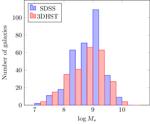
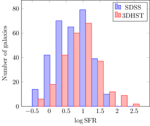
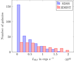
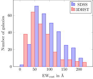
Figure 2: Histograms of the stellar mass, star formation rate, H$\beta$ luminosity, and rest-frame H$\beta$ equivalent width for the HST-selected star-forming galaxies at $z\sim 2.1$ and a set of local SDSS systems matched in stellar mass and star formation rate. Although the two distributions are different in detail, they both cover similar regions in mass–SFR–emission line phase space.

Table 2 summarizes the properties of all our $1.90<z<2.35$ 3D-HST galaxies. As the top left panel of Figure 2 shows, our sample of grism-selected star-forming galaxies have a wide range of stellar mass, extending from $\sim 10^{10}M_{\odot}$ to values as low as $\sim 10^{7}\,M_{\odot}$. A local SDSS galaxy sample is also shown in the figure; these comparison data, along with the other panels of the figure, will be described below.

4 The UV Continuum and Nebular Extinction

The wavelength range of our grism spectroscopy includes all the rest-frame optical emission lines blueward of $\sim 5100$ Å, so, in theory, we could obtain an estimate of nebular reddening directly from the Balmer decrement. In practice, however, H$\gamma$ and the higher-order Balmer lines are generally too weak (and too close in wavelength to H$\beta$) to produce a reliable measure of extinction. Thus, in the absence of H$\alpha$ measurements, we must rely on the stellar spectral energy distribution to constrain the nebular extinction.

Although our SED fits do produce a measure of stellar extinction, these values are subject to the multitude of assumptions associated with full spectrum SED modeling. A much more direct path to the stellar reddening, which is more reproducible by the reader and less subject to catastrophic errors, is to simply use the slope of the UV continuum between 1250 Å and 2600 Å. Because all of our $z\sim 2.1$ galaxies are undergoing vigorous star formation, their slope in this spectral range is well-approximated by a power law, i.e.,

$$F(\lambda)\propto\lambda^{\beta_{0}}$$ (1)

where $\beta_{0}=-2.25$ for populations which have been forming stars for more than $\sim 0.5$ Gyr, and is only slightly steeper for younger systems (Calzetti, 2001). We therefore adopt $\beta_{0}=-2.25$ for our analysis; if the UV slope is observed to be flatter than this, then the most-likely explanation is obscuration due to dust.

Translating the observed power-law slope into a measure of total (stellar) extinction at 1600 Å and total (nebular) reddening requires a number of assumptions. The most common assumption is that based on the work of Calzetti (2001), who showed that in the starbursting galaxies of the local universe, the observed slope of the rest-frame UV continuum, $\beta$, is related to the total stellar extinction at 1600 Å by

$$A_{1600}=\kappa_{\beta}\left(\beta-\beta_{0}\right)$$ (2)

with $\kappa_{\beta}=2.31$. Calzetti (2001) also showed that for nebular emission lines, a screen-model reddening law, such as that detailed by Cardelli et al. (1989) is appropriate, and that the amount of extinction affecting the gas is greater than that for the stars, so

$$E(B-V)_{\rm stars}=0.44E(B-V)_{\rm gas}\quad{\rm and}\quad A_{{\rm H}\beta}=\zeta_{{\rm H}\beta}A_{1600}$$ (3)

where $\zeta_{{\rm H}\beta}=0.83$. Whether this behavior continues at high redshift is uncertain: while a number of surveys have presented evidence for the applicability of this law at $z\sim 2$ (Förster Schreiber et al., 2009; Mannucci et al., 2009; Wuyts et al., 2013; Price et al., 2014; Holden et al., 2014; Zeimann et al., 2014), counter examples do exist (e.g., Erb et al., 2006; Kashino et al., 2013).

For consistency with other high-$z$ studies, we use the Calzetti (2001) obscuration law for our analysis. For the emission-line selected galaxies considered here, this law implies a median nebular extinction of $E(B-V)_{\rm gas}=0.21$. Note that if we were to assume that the Calzetti (2001) law systematically under-predicts the color excess of the gas by $E(B-V)_{\rm gas}\sim 0.1$, our median galactic oxygen abundance would increase by only 0.14 dex (see below). Similarly, if instead of applying an individual extinction correction to each galaxy, we were to adopt $E(B-V)_{\rm gas}=0.2$ for the entire sample, or used the Garn & Best (2010) correlation between extinction and stellar mass, our results would be qualitatively similar. Finally, the $E(B-V)$ obtained from the UV slope is systematically lower by $\sim 0.13$ dex than that obtained from SED fitting. Once again, this difference is small enough that it does not affect our conclusion.

5 Galactic Star-Formation Rates

Our SED analysis also produces a measure of star formation rate that is time-averaged over the history of the galaxy. To obtain an estimate of a system’s present-day SFR, we have two choices: we can use our grism measurements of the H$\beta$ line, which is produced by the recombination and cascade of electrons photo-ionized by hot $M\gtrsim 10\,M_{\odot}$ stars, or we can rely on the photometry of the rest-frame UV continuum, which traces the starlight from objects with $M\gtrsim 5\,M_{\odot}$. The advantage of the former method is that H$\beta$ records an “instantaneous” SFR, since only stars with ages less than $\sim 10$ Myr contribute to its emission (Kennicutt & Evans, 2012). A major disadvantage, however, is that H$\beta$ is rather weak in our spectra, and its measurement can be affected by underlying stellar absorption. (Zeimann et al. 2014 has shown that this equivalent width correction is likely to be small in our grism-selected galaxies, but it is still present.) Moreover, although the method is well-calibrated in the local universe (Hao et al., 2011; Murphy et al., 2011; Kennicutt & Evans, 2012), it is much more sensitive to metallicity than some other techniques, and this can lead to factor of $\sim 2$ errors at $z\sim 2.1$ (Zeimann et al., 2014). Finally, without knowledge of the Balmer decrement, SFR corrections for internal extinction can be problematic, as it is well known that the dust column that affects galactic emission lines is systematically greater than that which reddens starlight (e.g., Charlot & Fall, 2000; Calzetti, 2001). Since our measurement of extinction is limited to the slope of the rest-frame UV continuum, our knowledge of intrinsic H$\beta$ luminosities is indirect at best.

The alternative approach is to use the brightness of the rest-frame UV continuum as a measure of star formation rate. UV measurements are more sensitive to extinction as those of H$\beta$ (see equation 3), and the method traces star formation over a timescale that is $\sim 10$ times longer (e.g., Kennicutt & Evans, 2012) than that traced by the Balmer lines. However, its calibration is much less sensitive to metallicity variations than that for emission-line SFR indicators (Zeimann et al., 2014), and in most cases, the UV photometry of Skelton et al. (2014) has a higher signal-to-noise than our grism spectroscopy (H$\beta$ has a S/N $<2$ on average). We therefore adopt the de-reddened continuum flux density at rest-frame 1600 Å as our primary SFR indicator, with the calibration given by Kennicutt & Evans (2012) (originally tabulated in Murphy et al., 2011 and Hao et al., 2011) as our transformation coefficient. Figure 2 shows the distribution of these star formation rates.

Since most local universe SFR measurements are based on Balmer-line emission, and since the SFRs tabulated in the Sloan Digital Sky Survey (SDSS) Data Release 7 MPA-JHU galaxy catalog are based on H$\alpha$, we will examine if this choice of SFR indicator affects our conclusions about the $z\sim 2.1$ MSZ relation.

6 Emission Line Fluxes

For the redshift range under consideration, the HST grism spectra contain six strong emission lines: [O II] $\lambda 3727$, [Ne III] $\lambda 3869$, H$\gamma$, H$\beta$, and [O III] $\lambda\lambda 4959,5007$. To measure their fluxes, we began with the assumption that each spectrum could be fit via a series of Gaussian-shaped emission line profiles superimposed on a fourth-order ($n=4$) polynomial continuum. In other words, we assumed the intrinsic spectrum could be modeled via

$$f(\lambda)=\sum_{i=0}^{n}c_{i}\lambda^{i}+\sum_{j=n+1}^{n+k}\frac{c_{j}}{\sqrt{2\pi}\sigma}\exp\left(-\frac{(\lambda-\lambda_{e,j})^{2}}{2\sigma^{2}}\right)+w(\lambda)$$ (4)

where $w(\lambda)$ represents Gaussian white noise at each wavelength, the values $\lambda_{e}=(1+z)\,\lambda_{0}$ are the observed wavelengths of the $k=6$ fitted lines, and the values of $c_{j}$ encode the strengths of those lines. Following Storey & Zeippen (2000), the ratio of the [O III] doublet was fixed at 2.98:1. We then considered the fact that the data generated by the G141 grism are undersampled, so that each point in the measured spectrum, $F(x)$, is actually the integral of the model function over the size of the pixel $\Delta x$, i.e.,

$$F(x)=\int_{x-\Delta x/2}^{x+\Delta x/2}\,f(\lambda)d\lambda$$ (5)

We fit the observed spectrum to this model $F(\vec{x})$ via the maximum likelihood method. A full description of this procedure is given in the Appendix, and sample fits are shown in Figure 3. Finally, to correct for stellar absorption we augmented the H$\beta$ fluxes using the Balmer absorption line equivalent widths derived from our best-fit model SEDs. The derived line fluxes for all the $1.90<z<2.35$ galaxies are presented in Table 1, and a histogram of H$\beta$ luminosities is displayed in Figure 2.

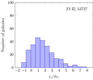
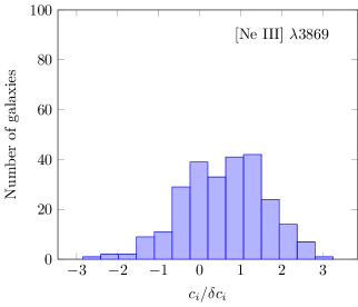
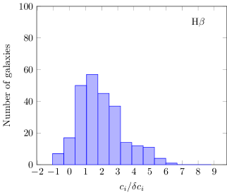
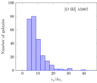
Figure 4: Histograms for the ratio of measured line flux $c_{i}$ to uncertainty $\delta c_{i}$ for [O II] $\lambda 3727$, [Ne III] $\lambda 3869$, H$\beta$, and [O III] $\lambda 5007$ for our $z\sim 2.1$ galaxies. Since these systems were selected via the blended [O III] doublet, the minimum $c_{i}/\delta c_{i}$ for [O III] is three. Since the signal-to-noise is quite low for some of our galaxies, stochasticity demands that some of the measured fluxes $c_{i}$ are negative. Thus, measuring metallicity can be quite challenging. Nevertheless, because the redshift is fixed by [O III], line fluxes can be measured to much lower signal-to-noise, although with large statistical uncertainties. Our Bayesian approach to metallicity determinations (see §7) accounts for this uncertainty, and we propagate the full p.d.f. of each measurement into our final analysis.

The galaxies in our program are generally very faint, with $22\lesssim m_{H}\lesssim 26$, hence the signal-to-noise in the grism data is often quite low. However, as described in §2, our galaxies were primarily selected via the presence of the distinctively shaped blended doublet [O III] $\lambda\lambda 4959,5007$. This fixes the redshift of each object, and allows us to measure lines such as H$\beta$, [O II] $\lambda 3727$, and [Ne III] $\lambda 3869$ to a very low signal-to-noise. Histograms of the ratio of the measured line fluxes $c_{i}$ to their formal statistical uncertainties $\delta c_{i}$ are shown in Figure 4. Note that $c_{i}$ is not the true value of the emission line flux, nor is $\delta c_{i}$ the uncertainty on this value. Rather, they are the observed realizations of the true signal $S$ and the noise in the measurement, $N$. In the limit where $S/N\gg 1$, the ratio $c_{i}/\delta c_{i}\rightarrow S/N$, but for faint sources, the stochasticity will dominate, resulting in some objects having values of $c_{i}<0$. Our Bayesian approach to metallicity determination properly accounts for these low S/N measurements and the resultant probability distribution functions for metallicity are propagated throughout our analysis (see §7).

Our $z\sim 2.1$ galaxies are all undergoing vigorous stellar formation. The best way to illustrate this fact is through the distribution of H$\beta$ emission-line equivalent widths. For the vast majority of our $z\sim 2.1$ objects, the HST grism spectra do not go deep enough to reliably detect the stellar continuum. Nevertheless, we can compare the strengths of our observed emission-line fluxes to the objects’ stellar continua via the HST’s broadband infrared photometry. We began by taking each galaxy’s F140W magnitude, and subtracting the contribution of all the emission lines falling into its bandpass. We then scaled the emission lines to our photometrically-estimated continuum measurement, i.e.,

$${\rm EW}_{{\rm H}\beta}=\frac{c_{{\rm H}\beta}}{f_{\rm F140W}\Delta\lambda-\sum_{i}c_{i}}\,\Delta\lambda$$ (6)

where the bandwidth of the F140W filter is $\Delta\lambda=3840$ Å, the values of $c_{i}$ represent the monochromatic fluxes of the emission lines falling within the filter (see the appendix), and $f_{\rm F140W}$ is the system’s $H$-band flux density. Each observed equivalent width was then divided by $1+z$ to obtain its value in the rest frame. These values are displayed (along with their uncertainties) in Figure 3 of Zeimann et al. (2014). To examine the true distribution of H$\beta$ emission-line equivalent widths, we correct our values for the Balmer absorption of the stars using our best-fit model for the SED. Finally, we also correct for the difference between stellar and nebular reddening via the Calzetti (2001) relation $E(B-V)_{\rm stellar}=0.44E(B-V)_{\rm gas}$.

Obviously, equivalent widths derived from a combination of spectroscopy and broadband photometry can carry a significant uncertainty. In particular, for many of our program galaxies, the contribution of [O III] $\lambda 5007$ to the F140W flux density is substantial, so for the faintest objects, the H$\beta$ line’s equivalent width is poorly known at best. In fact, it is these objects which dominate the low-EW end of the histogram displayed in Figure 2. All the well-measured galaxies in our sample have H$\beta$ equivalent widths greater than 30 Å, and most have EW${}_{{\rm H}\beta}>50$ Å. The objects detected by the G141 grism are clearly dominated by on-going star formation.

7 Deriving Gas-Phase Metallicities using Local Counterparts

Our $z\sim 2.1$ grism observations do not reach the weak nebular lines of [O III] $\lambda 4363$ and He II $\lambda 4686$. Consequently, the only way to translate our bright-line emission fluxes into gas-phase metallicities is to do so differentially, using systems with well measured oxygen abundances as a control sample. By examining the behavior of the bright emission lines as a function of nebular abundance, one can define a metallicity calibration that can be applied to the galaxies of the distant universe.

Unfortunately, such a procedure is fraught with difficulties. Perhaps the most commonly used set of strong-line metallicity calibrations are those derived by Maiolino et al. (2008), who combined direct abundance measurements for $\sim 300$ low-metallicity galaxies (see Nagao et al., 2006) with photoionization-model based abundances for $\sim 22,000$ high-metallicity systems (Kewley & Dopita, 2002). However, the applicability of these relations to our study is unclear, as the physical conditions within most nearby galaxies are significantly different from those found in the high-redshift universe. On average, $z\sim 2$ galaxies form stars ten times more rapidly than do local objects (Whitaker et al., 2014), and as discussed earlier, they tend to have harder ionizing fields (Steidel et al., 2014), higher ionization parameters (Nakajima & Ouchi, 2014), and higher nebular densities (Shirazi et al., 2014) for the same stellar mass. Consequently, the use of abundance calibrations that are based on magnitude-limited samples defined from ensembles of low-$z$ galaxies may not be appropriate. This is especially true at the poorly-populated, low-luminosity, metal-poor end of the distribution ($12+\log({\rm O}/{\rm H})<7.7$), where the Maiolino et al. (2008) sample contains just a small handful of objects.

7.1 The Local Stellar Mass- and SFR-Matched Sample

Rather than use the entire SDSS catalog, which includes galaxies with star formation rates and masses that are vastly different from those found in our $z\sim 2.1$ galaxy sample, we chose to follow the example of Izotov et al. (2006) and compare to a set of galaxies whose global properties are similar to those of our $z\sim 2.1$ systems. To define this sample, we began with the table of emission line fluxes, stellar masses, and star formation rates provided by the Sloan Digital Sky Survey (SDSS) Data Release 7 MPA-JHU galaxy catalog. We then selected those galaxies with H$\beta$ luminosities greater than $L_{{\rm H}\beta}\geq 3\times 10^{40}$ ergs s^-1, and positive monochromatic emission line fluxes for [O II] $\lambda 3727$, [Ne III] $\lambda 3869$, H$\beta$, and [O III] $\lambda 5007$. After excluding objects with unusually strong [O III] $\lambda 4363$ or [N II] $\lambda 6584$, or line ratios that suggested the presence of an AGN (Kauffmann et al., 2003), we went through each $z\sim 2.1$ galaxy in our sample and identified the five SDSS galaxies closest to it in $\log M_{*}$-$\log$ SFR space. (In the median, these “matched” galaxies were all within 0.12 dex of their $z\sim 2.1$ counterpart.) Since some SDSS galaxies are associated with more than one $z\sim 2.1$ system, the resulting “matched” dataset consisted of 319 local galaxies.

Necessarily, this procedure of identifying counterparts to our $z\sim 2.1$ grism-selected galaxies is not ideal. Unlike our COSMOS and GOODS galaxies, which have comprehensive rest-frame UV through rest-frame IR photometry in up to 44 separate bandpasses (see §3), the photometric data for the local objects are limited to the 5 SDSS bandpasses, $ugriz$. Consequently, the cataloged SED-based masses are not as robust as those for the distant galaxies. Similarly, the SFR estimates for the SDSS galaxies are based on H$\alpha$ (Brinchmann et al., 2004), while those for the $z\sim 2.1$ objects rely on photometry of the rest-frame UV. While both techniques are well-calibrated in the local universe (e.g., Kennicutt & Evans, 2012), their effective timescales are different (see §5). Finally, it is well-known that galaxies at high redshift generally have systematically higher SFRs than local systems (e.g. Madau & Dickinson, 2014; Whitaker et al., 2014), and, despite our best attempts to minimize the discrepancy, this causes our $z\sim 2.1$ systems to extend over a wider range in stellar mass-SFR space than the local matched sample. As we will show below, we can address this problem by restricting our comparison to galaxies with the same mass-SFR bin. Nevertheless, it is a fundamental limitation of the matched sample.

The propriety of local mass- and SFR-matched sample of high line-luminosity galaxies is illustrated in Figure 5. From the figure, it is clear that the envelope defined by our local matched sample and the set of $z\sim 2.1$ grism-selected galaxies extend over the exact same region in emission-line ratio phase space ([O III]/[O II] vs. $R_{23}$). Moreover, at high metallicity, the line ratios of both galaxy samples follow the track defined by the commonly-used metallicity calibration of Maiolino et al. (2008). However, in the lowest metallicity systems ($12+\log{\rm(O/H)}<7.7$), the Maiolino et al. (2008) relations are not a good match to the data, as they extend into a region of phase space that is not populated by either dataset. Clearly, in the low-metallicity regime, a more robust calibration is needed.

7.2 Strong Line Abundance Calibrations from the Local Sample

All but 47 of the galaxies in the local sample have measurements of the auroral [O III] $\lambda 4363$ line that are at least twice that of its flux error. For these 272 objects, we can determine electron temperatures directly, and hence derive a physics-based estimate of their gas-phase metallicity (Osterbrock & Ferland, 2006; Izotov et al., 2006). Using these data, we could obtain a new set of polynomial relations relating the galaxies’ bright emission-line ratios to these abundances.

To do this, we began by assuming that, due to the range of possible physical conditions within bright H II regions, there is no unique relation between line ratio and metallicity. Instead, we assumed that a system with metallicity $Z$ can have a range of line ratios, with the probability of observing any given line-ratio, $R$, defined as a Gaussian, with a mean $\log R_{i}(Z)=r_{i}(Z)$ and a dispersion $\sigma_{r_{i}}$. Here, $r_{i}(Z)$ is a low-order polynomial, representing the behavior of the index versus metallicity. In other words, the probability of observing a line ratio, $R_{i}$, in a galaxy whose true metallicity is $Z$ is given by the Gaussian distribution function $p(\log R_{i})=(2\pi\sigma_{r_{i}}^{2})^{(-1/2)}\,\exp(-(\log R_{i}-r_{i}(Z))^{2}/2\sigma_{r_{i}}^{2})$. We then used the method of maximum likelihood to solve for the polynomial coefficients of $r_{i}(Z)$ and $\sigma_{r_{i}}$ for the various line ratios associated with the forbidden lines of oxygen, neon, and nitrogen. The coefficients for these fits, along with the most-likely value of $\sigma_{r_{i}}$, are given in Table 3 and displayed in Figure 6. Also shown in Figure 6 are the more established relations of Maiolino et al. (2008). As expected, due to the physics of nebular cooling and stellar opacities, the fits for the [O III]/H$\beta$, [O II]/H$\beta$, and the $R_{23}$ relation required a quadratic term (e.g., Kewley & Dopita, 2002; Kewley et al., 2013; Levesque & Richardson, 2014); for the other line ratios, linear fits were sufficient.

It is important to note that for our sample of mass-SFR matched, high line-luminosity objects, our new relations are quite similar to those of Maiolino et al. (2008), except in the regime where the oxygen abundance dips below $12+\log({\rm O/H})<7.8$. At these very low metallicities, the Maiolino et al. (2008) relations are defined by literature measurements of roughly two dozen local, heterogeneously selected galaxies (see Nagao et al., 2006). In terms of numbers, our local sample is no better, with only $\sim 4$ objects in this low-metallicity range. However, because we selected our local galaxies to match the $z\sim 2.1$ systems’ star formation rates and stellar masses, it is likely that the physical conditions in these systems are a better match to the high redshift counterparts. We therefore adopted these new calibrations for both the $z\sim 2.1$ galaxies and our local comparison sample, and use them in our analysis.

7.3 Deriving Metallicities

To translate our emission line fluxes into galactic metallicities, we began by choosing three strong-line abundance indicators for analysis: $R_{23}$, [O III]/[O II], and [Ne III]/[O II]. (Other combinations of indicators are possible, but as long as the degrees of freedom are reduced to the minimum, the results of each set of indicators are consistent.) We used the re-calibrated versions of these relations discussed in §7.2 to construct a “meta-indicator”, that, given a metallicity and extinction, simultaneously predicts the relative values of all the strong-line fluxes. We then adopted a nebular extinction law (Cardelli et al., 1989), used the slope of the UV continuum to obtain an estimate of the total extinction at H$\beta$ (see §4), corrected our line fluxes for this reddening while fixing the H$\gamma$/H$\beta$ ratio to 0.47 (Hummer & Storey, 1987), and applied the metallicity calibrations shown in Figure 6. Finally, we computed the likelihood that any given galaxy with oxygen abundance $12+\log({\rm O/H})$ would possess the line fluxes given in Table 1.

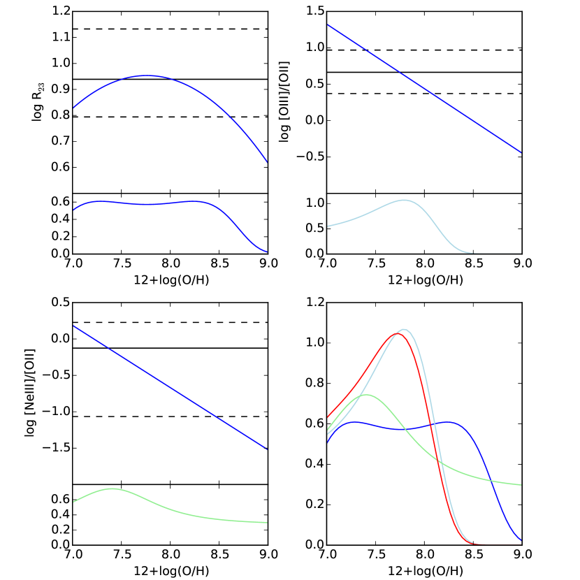
Figure 7: A demonstration of how the different indicators contribute to the metallicity estimate for one of the galaxies in our sample. The lower curves in the upper left ($R_{23}$), upper right ([O III]/[O II]), and lower left ([Ne III]/[O II]) panels show the likelihood distributions for each indicator, normalized in the range $Z=7-9$. These were derived by predicting the relative line fluxes using the polynomial relationships between line ratio and metallicity (upper solid blue curve), and then comparing these ratios to the measured best-fit line fluxes and their associated uncertainties. The solid black line shows the best fit ratio, with the 16th and 84th-percentiles illustrated as dashed lines. The bottom right panel repeats these probability distributions ($R_{23}$ in blue, [O III]/[O II] in teal, and [Ne III]/[O II] in green) and shows the probability distribution function for the combined three-ratio meta-indicator in red.

The details of this procedure are explained in the Appendix. The constraining power added by each indicator is illustrated in Figure 7, where we show the metallicity solution for one of the galaxies in our sample. In the figure, the solid black horizontal lines and their surrounding dashed lines represent the de-reddened values for $R_{23}$, [O III]/[O II], and [Ne III]/[O II], and their uncertainties. For comparison, the blue curves display the metallicity calibrations shown in Figure 6. Because in the construction of the likelihood function, the predicted variance depends on both metallicity and line flux (see Appendix), the most likely metallicity is not necessarily at the exact location where the black line and blue curves intersect (though it is close). The lower section of each plot displays the likelihood that the observed line ratio is the product of a given metallicity. These likelihoods were normalized in the metallicity range 7–9, and are reproduced graphically in the lower-right hand panel of the figure, along with the likelihood derived from the combined meta-indicator. For this particular object, it is apparent that the $R_{23}$ index does not provide a strong constraint on metallicity, as the probability density distribution function is broad and slightly double-peaked. The [O III]/[O II] ratio helps constrain this peak, as does (to a lesser extent) the ratio of [Ne III] relative to [O II].

To test our maximum-likelihood procedure, we applied our code to the emission lines of the local calibration galaxies. The results are displayed in Figure 8, where we compare the metallicities computed from our meta-indicator against those derived via “direct” analyses using the temperature sensitive auroral [O III] $\lambda 4363$ line. Although there may be a slight trend in the data, a maximum likelihood analysis assuming constant scatter yields a slope of $0.998\pm 0.050$, and, on average, the offset between the two abundances is $\log({\rm O/H})_{\rm strong-line}-\log({\rm O/H})_{\rm direct}=0.028\pm 0.154$ dex. This is significantly better than the results which would be obtained using the Maiolino et al. (2008) relations ($-0.041\pm 0.148$ dex), though the scatter about the one-to-one line is slightly higher. The fact that there is a very small, metallicity-dependent trend in the residuals is due to our use of a first-order polynomial for the [O III]/[O II] component of the measurement. A second-order polynomial fit would remove this trend, but it would also cause our meta-indicator to become less reliable for low signal-to-noise objects.

Figure 3 illustrates the dependence of our abundance estimates on nebular extinction. The most obvious feature to note is the lack of direct constraints on reddening. In many cases, this leads to double-valued solutions: a metal-poor solution, where the relative weaknesses of [O II] $\lambda 3727$ and [Ne III] $\lambda 3869$ are presumed to be intrinsic, and a metal-rich ($\sim$ solar metallicity) solution, where the short wavelength lines are assumed to be depressed by extinction. Conversely, for many galaxies the oxygen abundance is reasonably well defined even without a reddening constraint, with typical fitting errors of $\sim 0.8$ dex. The application of a stellar continuum-based reddening constraint (Calzetti, 2001) then reduces this uncertainty to $\sim 0.4$ dex.

8 The (Non-) Fundamental Mass–Metallicity–SFR Relation

In §1, we discussed the numerous investigations aimed at measuring the relationship between stellar mass, star formation rate, and metallicity in the $z\sim 2$ universe. At the same time, there has been a similarly large effort concerning the Fundamental Metallicity Relation of the local universe, with various authors choosing to emphasize differences in their sample selection, stellar-mass and SFR coverage, abundance calculations, and empirical fitting functions (e.g., Lara-López et al., 2010; Mannucci et al., 2010, 2011; Andrews & Martini, 2013; Lara-López et al., 2013; de los Reyes et al., 2015). For example, Lara-López et al. (2010) used 32,575 SDSS galaxies and the Tremonti et al. (2004) metallicity calibration to argue for the existence of a fundamental plane in $M_{*}$-SFR-$Z$ space that holds out to $z=3.5$, and an update using a volume-selected sample from the SDSS and the Galaxy and Mass Assembly (GAMA; Driver et al., 2011) surveys obtained the same result (Lara-López et al., 2013). In contrast, an analysis by Mannucci et al. (2010), which used the Maiolino et al. (2008) $R_{23}$ and [N II]/H$\alpha$ abundance estimators and a less restrictive selection sample of these same SDSS DR7 galaxies found that $z\sim 0.1$ galaxies fall not on a plane, but on a second order surface that is non-evolving out to $z=2.5$. Further complicating the issue is a study by Andrews & Martini (2013), who applied a spectral stacking algorithm to a large number of SDSS galaxies, in order to detect the temperature-sensitive weak [O III] $\lambda 4363$ auroral line and thereby directly measure metallicities. The Andrews & Martini (2013) $M_{*}$-SFR-Z measurements are not consistent with the fundamental plane of Lara-López et al. (2013) nor with the fundamental surface of Mannucci et al. (2010). While some of the differences between these studies can be attributed to systematic uncertainties of up to 0.7 dex between strong line abundance indicators (Kewley & Ellison, 2008), a full explanation of these discrepancies still does not exist.

Despite these problems, a comparison between local and high-redshift abundance estimates can still hold meaning, as long as the measurements are performed carefully in a self-consistent manner. As shown in Figure 5, both sets of galaxies inhabit the same regions of emission-line space, allowing the calibrations derived in §7.2 to be applied to both datasets in the same manner. This should reduce systematic errors to a minimum.

We created our $z\sim 2.1$ MSZ relation following the procedures described above. The metallicities of our galaxies were computed by combining the information from our three abundance sensitive line ratios, computing each galaxy’s 2-dimensional probability distribution function in extinction–metallicity space, and then marginalizing over extinction using the stellar reddening measurements obtained from the UV slope, the Calzetti (2001) prescription relating stellar and nebular attenuation, and the Cardelli et al. (1989) extinction law. While other prescriptions for the stellar reddening curve and the relationship between stellar and nebular reddening are possible (e.g., Buat et al., 2012; Scoville et al., 2015; Price et al., 2014; Reddy et al., 2015), their use makes very little difference to the final result. Our stellar mass determinations were obtained from SED fitting (see §3), and our estimates of SFR were derived using the reddening corrected photometric measurements of the objects’ UV continua and the Kennicutt & Evans (2012) SFR calibration (§5). These measurements are summarized in Table 2.

One common way to visualize MSZ results is by plotting metallicity as a function of a projection in SFR and stellar mass. Unfortunately, while this procedure reduces the dimensionality of the data and allows for easy viewing, it ignores much of the information by averaging over the direction of projection. For example, when plotting our galaxies’ metallicity versus stellar mass, both our $z\sim 2.1$ and local matched samples appear to agree very well with the Dayal et al. (2013) model, and the same is true when using the “ideal projection” ($\mu_{0.32}=\log M_{*}-0.32\log{\rm SFR}$) found by Mannucci et al. (2010) in the local universe. The projection washes out any metallicity gradient that may be present.

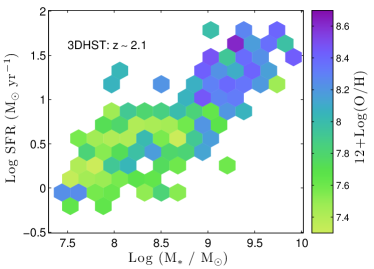
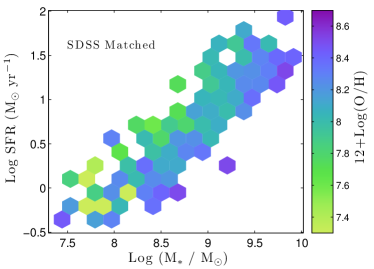
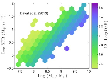
Figure 9: Three panels showing the relationship between stellar mass, star formation rate, and metallicity for $z\sim 2.1$ galaxies (upper left), a local sample of SDSS galaxies matched in stellar mass and star formation rate (upper right), and the non-evolving Dayal et al. (2013) chemical evolution model. The metallicities of the two samples of galaxies have been determined in the same way using our new polynomial relations (see §7.2). The data have been binned into 0.102 dex hexagons, and only those bins with at least one galaxy have been plotted. In the local sample, there is a metallicity gradient that runs roughly perpendicular to the $M_{*}$-SFR correlation that follows the predictions of the Dayal et al. (2013) model. This gradient is in a different direction at $z\sim 2.1$.

A better way to visualize the galaxies in three-dimensional $M_{*}$-SFR-$Z$ space, while correctly propagating the uncertainties associated with each abundance estimate, is to view the $M_{*}$-SFR plane from “above” and use color to represent metallicity. To do this we began by binning our galaxies into hexagonal regions with radii of 0.102 dex in $\log M_{*}$ and $\log{\rm SFR}$. We then took the probability contours computed from our metallicity analysis, convolved them with the uncertainties associated with reddening and SFR, and color-coded each hexagon according to the expectation value for metallicity. The resulting metallicity maps for our set of $z\sim 2.1$ HST grism-selected galaxies, and our SDSS sample of stellar mass and star formation rate matched systems are shown in Figure 9.

The results of Figure 9 can be interpreted using some of the theoretical models that have been developed to explain a non-evolving relationship between $M_{*}$-SFR-$Z$ (e.g., Davé et al., 2012; Dayal et al., 2013; Lilly et al., 2013; Pipino et al., 2014; Forbes et al., 2014). Perhaps the most instructive of these is the simple, redshift-independent analysis by Dayal et al. (2013), whose instantaneously-recycling model takes into account star formation, inflows from the metal-poor IGM gas, and outflows of metal-enhanced ISM gas. The basic assumptions of this model are that star formation is proportional to gas mass, outflows are driven by star formation via winds and supernovae, and that inflows increase gas mass and hence trigger star formation. There are two main parameters of this model — the inflow rate and the outflow rate — and factors of proportionality depend on halo mass, which to first order is proportional to stellar mass (Dayal et al., 2009). One way to interpret this model is therefore through perturbation theory, since the star formation rate is small compared to the timescale over which gas dynamics takes place. Mergers are not included in this analysis, as Mannucci et al. (2010) has argued that a large number of such events would produce a much higher scatter about the mass–metallicity relation than is observed locally. The predictions of this model are also shown in Figure 9.

>From Figure 9, it is clear that all three panels confirm the existence of the well-known correlations between mass and star formation rate, and mass and metallicity. The local mass- and SFR-matched sample of vigorously star-forming SDSS galaxies also exhibits a metallicity gradient that is approximately perpendicular to the $M_{*}$-SFR relation: objects with high stellar mass and low SFR have a higher than average metallicity. This trend is easily seen in the Dayal et al. (2013) model, but it is not obviously visible in our grism-selected sample. Instead, the metallicity gradient at $z\sim 2.1$ is roughly parallel to the $M_{*}$-SFR relation, with higher metallicities associated with systems with higher masses and higher star formation rates.

• Using new metallicity relations: UV SFR:
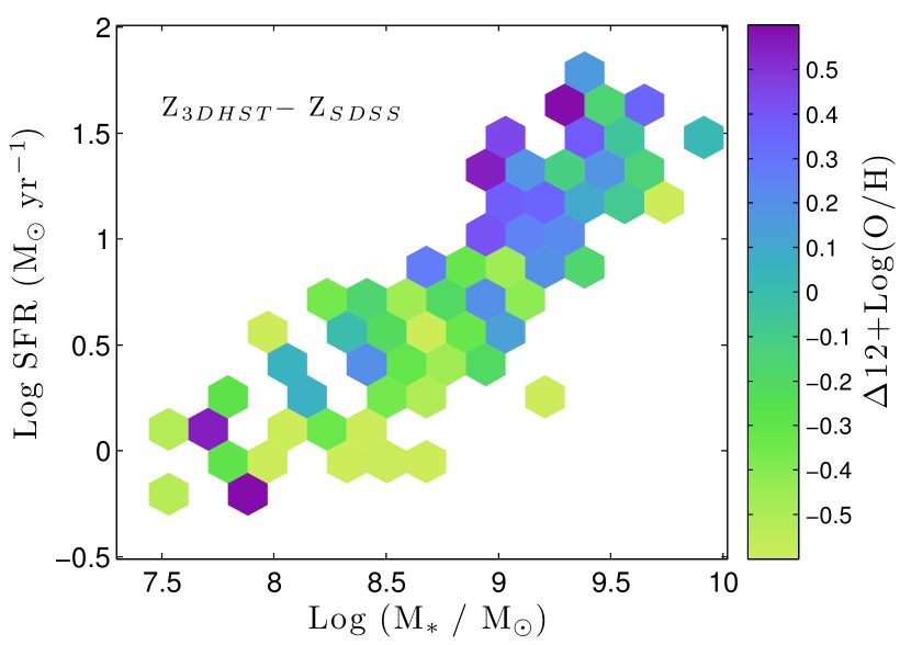
H$\beta$ SFR:
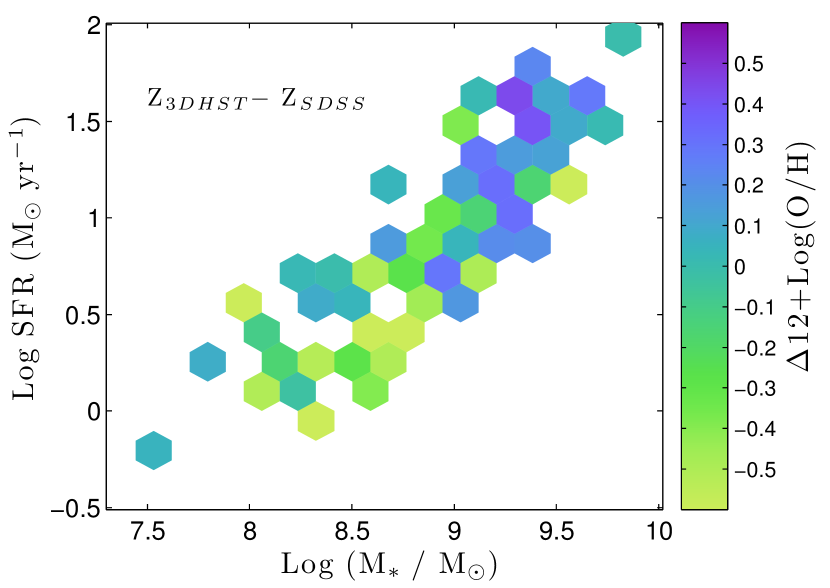
• Using Maiolino et al. (2008) relations: UV SFR:
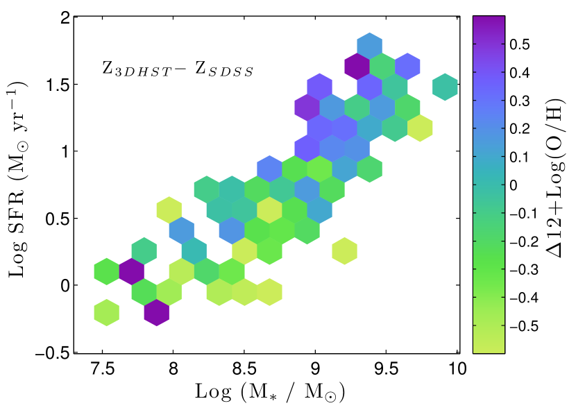
H$\beta$ SFR:

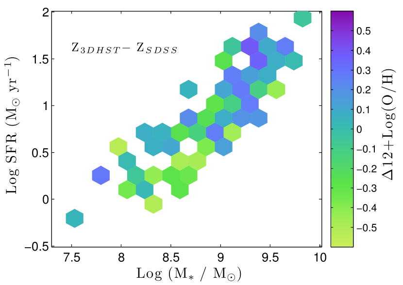
Figure 10: The difference between the metallicity measurements of $z\sim 2.1$ grism-selected galaxies and similar measurements for our local sample of high H$\beta$ line-luminosity galaxies matched in stellar mass and star formation rate. The data have been binned into 0.102 dex hexagonal pixel. The left column shows abundance estimates determined via the metallicity calibration derived from our local sample of galaxies, with the top panel showing the distribution using rest-frame UV photometry as our SFR indicator and the bottom plot using H$\beta$ to estimate the star formation rate. The right column repeats these plots using the Maiolino et al. (2008) relations to estimate metallicity. All four plots illustrate the same result: at stellar masses above $\sim 10^{9}\,M_{\odot}$ and star formation rates above $\sim 10\,M_{\odot}$ yr^-1 all but three of the bins have a higher metallicity at $z\sim 2.1$ than seen locally. At lower masses and SFRs, it is the nearby galaxies that are more metal-rich.

Another way of seeing the gradient is to subtract the metallicity of each hexagonal bin in the local matched sample from that calculated for the $z\sim 2.1$ galaxies. This is shown in the top-left of Figure 10, where only those bins with at least one galaxy in each sample have been plotted. The noise in the map comes principally from the HST grism data, which is of lower quality than the local SDSS measurements. Nevertheless, there is a clear pattern to the data: at stellar masses above $\sim 10^{9}\,M_{\odot}$ and star formation rates above $\sim 10\,M_{\odot}$ yr^-1, the $z\sim 2.1$ galaxies tend to have higher oxygen abundances than their local counterparts. In contrast, in the low-mass, low-SFR region of the diagram, most of the $z\sim 2.1$ bins have lower abundances than their corresponding nearby objects.

Figure 10 demonstrates that the same qualitative pattern is present when the relations of Maiolino et al. (2008) are used to determine metallicities, or if H$\beta$ luminosity is used to measure star formation rate in our $z\sim 2.1$ systems. Since the set of local mass- and SFR-matched SDSS systems described in §7.1 is a better match to the $z\sim 2.1$ grism-selected galaxies than the general ensemble of SDSS systems, we put more confidence in our new metallicity calibration than in the Maiolino et al. (2008) relations, but both produce the same trends. Similarly, because of the generally low signal-to-noise of our $z\sim 2.1$ H$\beta$ measurements, and because H$\beta$ SFRs are susceptible to shifts in metallicity (Zeimann et al., 2014), we prefer to use star formation rate measurements which are based on rest-frame UV photometry. But this choice does not affect our results.

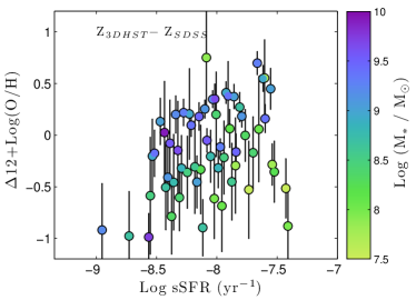
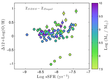
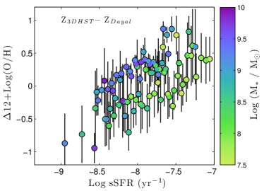
Figure 11: Residual metallicities between the $z\sim 2.1$ 3D-HST sample, our local SDSS comparison sample of high H$\beta$ line-luminosity galaxies matched in stellar mass and SFR, and the Dayal et al. (2013) model, as a function of mass-specific star formation rate (sSFR). Each data point represents one of the hexagons in Figure 9, colored by stellar mass. The error bars illustrate the statistical uncertainty of each bin. Top: Difference between the two samples. Only bins that have at least one galaxy in each of the two samples are shown. High-mass galaxies in the 3D-HST sample tend to have higher metallicities than the local SDSS matches. Lower left: The matched sample local counterparts compared to the Dayal et al. (2013) chemical evolution model. About half the scatter is explained by the dispersion about the metallicity calibrations (see §7.2), and some outliers are present. Lower right: Metallicity residuals between the 3D-HST sample and the Dayal et al. (2013) model. As in the previous plot, the 3D-HST galaxies tend to have lower metallicities at lower star formation intensities. However, at larger sSFRs, the 3D-HST galaxies have higher metallicities than the model. This is not seen locally, and is especially true for the higher-mass galaxies in the sample.

The top panel of Figure 11 displays these same data, along with their statistical error bars, as a function of mass-specific star formation rate. Once again, one can see the systematic behavior with mass, as galaxies above $\sim 10^{9}\,M_{\odot}$ tend to lie in the upper part of the figure, while those with masses below $\sim 10^{8.6}\,M_{\odot}$ mostly have lower metallicities. However, there is considerable noise in the diagram, as there are a limited number of galaxies in the samples, and certain sections of the mass-SFR-metallicity phase space are poorly populated. To help remedy this situation, the lower panels of Figure 11 difference the $z\sim 2.1$ and local galaxy results from the physically motivated Dayal et al. (2013) model that is well-calibrated locally using massive galaxies with low star formation. Since we use the strong-line metallicity indicators of §7.2, about half of the scatter in the figure can be explained by the imperfect nature of the relations. Nevertheless, for the local sample, it is clear that the Dayal et al. (2013) model does a reasonably good job at predicting metallicity, apart from a few outliers.

At $z\sim 2.1$, however, the situation is different. There is a strong correlation between the metallicity excess over the Dayal et al. (2013) model and the mass specific star formation rate. Galaxies which had intense star formation $\sim 3$ Gyr after the Big Bang have a higher gas-phase metallicity than their local counterparts. In addition, the high-mass galaxies of the epoch tend to have a metallicity over and above that predicted by the models, whereas the low-mass systems have fewer metals. Such offsets are not seen in the local universe.

Can the differences seen in Figures 9 through 11 be explained by systematic offsets caused by our choice of metallicity calibration, star formation rate indicator, or stellar mass estimator? As Figure 10 illustrates, the same patterns are present when the relations of Maiolino et al. (2008) are used instead of our own metallicity relations. Since our local calibration sample is a better match to the $z\sim 2.1$ grism-selected systems, we put more confidence in the plots of Figure 10 where we use the new strong-line calibrations from Table 3, but these relations are not the source of the change in direction of the gradient. Similarly, our use of UV-based star formation rates for the $z\sim 2.1$ dataset does not qualitatively change our results. H$\beta$ is usually weak in our grism-selected galaxies, and its measurement may be affected by underlying Balmer absorption. (Brinchmann et al. (2004) have argued that the derived SFRs for low-metallicity SDSS galaxies are still very good, even if this effect is neglected. Nevertheless, we have corrected our H$\beta$ emission-line fluxes using absorption line estimates derived from our best-fitting SED models.) If we then apply the same SFR conversion used for the SDSS galaxies (Brinchmann et al., 2004), we still see the same trends in the data. In order to attribute the differences in the $M_{*}$-SFR-$Z$ to errors in the star formation rate, the SFR in high-mass galaxies would need to be overestimated by no less than $\sim 0.5$ dex, while in low-mass galaxies, SFR would need to be underestimated by the same amount. This is exceedingly unlikely.

Analyzing the effect of errors in our stellar mass measurements is more difficult. As noted in §7.1, the SDSS stellar masses adopted for the local sample were based on 5-band $ugriz$ photometry, whereas our $z\sim 2.1$ mass measurements used the entire rest-frame UV through rest-frame IR SED. So systematic offsets between the two samples are possible. However, in order to attribute the differences in the $M_{*}$-SFR-$Z$ relation to this difference, a simple shift in stellar mass is not sufficient: one would need to have the $z\sim 2.1$ galaxy masses underestimated by a factor $\sim 10$ for high-mass galaxies, and overestimated by a similar factor for low-mass systems. Again, such errors are unlikely, though we would need a congruent local dataset with complete UV through near-IR photometry to completely exclude the possibility.

Finally, we need to consider whether the systematic trends observed in Figure 9 are due to changes in the physical conditions within the epochs’ H II regions. Because of the link between metal abundance and stellar opacity, there is a well-known correlation between the ionization parameter and metallicity (e.g. Kewley et al., 2013, and references therein). This, in part, defines the behavior of the strong-line metallicity indicators used in this paper. However, if this correlation changes between $z\sim 2.1$ and today, then our metallicity determinations could be in error. Again, this shift would need to cause us to overestimate the gas-phase abundances for our $z\sim 2.1$ high-luminosity, high-metallicity systems, while underestimating $Z$ in low-metallicity galaxies. We attempted to minimize this effect by creating a sample of local galaxies with physical conditions as close to those at $z\sim 2.1$ as possible. Nevertheless, we cannot fully rule out this possibility.

Despite our best effort to reduce systematics, we still see correlations between the metallicity offsets in stellar mass, SFR, and sSFR. On average over a large enough region of phase space, these offsets cancel out, but as it stands, the $M_{*}$-SFR-$Z$ surface defined by our $z\sim 2.1$ HST grism-selected galaxies is different from that of our local mass- and SFR-matched SDSS sample, and different from the physically-motivated model of Dayal et al. (2013).

9 Summary

In this study we examined the distribution of intensely star-forming $z\sim 2.1$ galaxies in stellar mass–SFR–metallicity space and compared our results to a sample of local galaxies. This study differs from previous investigations of this Fundamental Metallicity Relation in that it contains significant numbers of galaxies with low stellar mass ($7.5\lesssim\log(M/M_{\odot})\lesssim 10$), and high star formation rates $-0.5\lesssim\log{\rm SFR}\lesssim 2.5$ (in $M_{\odot}$ yr^-1). In total, we have 256 measurements of stellar mass, metallicity, and star formation in the $z\sim 2.1$ universe. To summarize our findings:

1. We calibrate the strong-line metallicity indicators using a local sample of emission line galaxies with high H$\beta$ luminosities ($L_{{\rm H}\beta}\geq 3\times 10^{40}$ ergs s^-1) and matched in stellar mass and star formation rate to our $z\sim 2.1$ sample. These galaxies obey the Maiolino et al. (2008) metallicity calibrations except at low metallicity, where our relations produce abundances that are lower by $\sim 0.15$ dex. This makes a difference for galaxies with masses below $\sim 10^{8.5}\,M_{\odot}$ (§7.2).

2. By combining several strong-line ratio metallicity indicators ($R_{23}$, [O III]/[O II], and [Ne III]/[O II]) into a single meta-indicator, we break the well-known degeneracy in the $R_{23}$ relation; this is important, since many of our galaxies lie close to the peak of the $R_{23}$ curve. The combination of indicators also significantly reduces the statistical error in our measurements.

3. In a metallicity map in $M_{*}$-SFR space (Figure 9), the metallicity gradient for the $z\sim 2.1$ HST-selected galaxies is along the $M_{*}$-SFR relation, whereas for the local galaxies, the gradient is roughly perpendicular to this correlation.

4. At masses above $\sim 10^{9}\,M_{\odot}$ and star formation rates above $\sim 10\,M_{\odot}$ yr^-1, star-forming galaxies at $z\sim 2.1$ have higher metallicities than similar objects in the local universe. At lower masses and star formation rates, the $z\sim 2.1$ systems tend to have lower metallicities than their local counterparts (Figure 10).

5. At $z\sim 2.1$, intensely star-forming galaxies have higher metallicities than predicted by the chemical evolution model of Dayal et al. (2013). Similar local galaxies only deviate from this model at very low specific star formation rates (Figure 11).

Figure 1: The redshift distribution of $1.90<z<2.35$ emission-line galaxies in the COSMOS, GOODS-N, and GOODS-S fields. The data show that the sample contains galaxies from the full redshift range.

Figure 3: Three galaxies that exemplify the range of fitting solutions for our sample of $z\sim 2.1$ grism-selected galaxies. The spectra on the left are shown with 1-$\sigma$ error bars, with the best-fitting model illustrated as a solid red line. The metallicity vs. $E(B-V)$ contours are shown on the right, marginalized over all nuisance parameters. In many cases, the metallicity is moderately well-determined, even if the reddening is not; in other cases, an estimate of extinction would greatly improve the abundance measurement. While we cannot measure nebular extinction directly, we can constrain $E(B-V)_{\rm gas}$ via measurements of stellar reddening and the Calzetti (2001) attenuation law.

Figure 5: The relationship between two of the three line ratios used to empirically determine gas-phase metallicity for our sample of $z\sim 2.1$ galaxies. The nearly 200,000 star-forming galaxies from the SDSS DR7 catalog are shown via the blue density plot, while our sample of $z\sim 2.1$ grism-selected galaxies is shown in red. (Only those galaxies where all four of our key emission lines have detections with S/N $>4$ have been plotted). The red error bar in the upper right corner is the median error of this sample. A local calibration sample, i.e., systems with H$\beta$ luminosities larger than $3\times 10^{40}$ ergs s^-1 and matched in stellar mass and SFR to our $z\sim 2.1$ systems are shown as green diamonds. For comparison, the black squares show the empirical relation of Maiolino et al. (2008), which extends from $12+\log({\rm O/H})=9.0$ to 7.0 in 0.2 dex intervals. Within the measurement errors, our galaxies occupy the same emission-line phase space as the local calibration sample, while the Maiolino et al. (2008) calibrations deviate significantly from this locus at low metallicity.

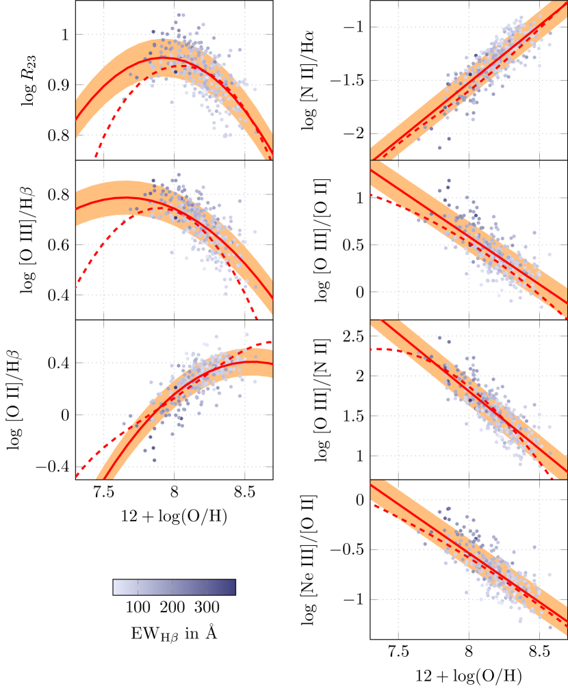
Figure 6: The gas-phase oxygen abundances versus strong emission-line ratios for our local calibration sample of high luminosity ($L_{H\beta}>3\times 10^{40}$ ergs s^-1), mass- and SFR-matched galaxies. The objects are color-coded by their rest-frame equivalent width. The solid red lines show the polynomial fits for our calibration sample, with the scatter indicated by the orange-shaded area (Table 3). The dashed red lines are the Maiolino et al. (2008) relations.

Figure 8: The metallicities obtained using our meta-indicator of three line ratios, $R_{23}$, [O III]/[O II], and [Ne III]/[O II] (see Table 3) compared to physics-based abundances determined using the electron temperature sensitive [O III] $\lambda\lambda 4959,5007$/[O III] $\lambda 4363$ line ratio. The dashed red line depicts where the abundances match. On average, strong-line metallicity estimates are greater than the direct abundances by $0.028\pm 0.154$ dex; this agreement is better than that for the Maiolino et al. (2008) relations ($-0.041\pm 0.148$ dex), though the scatter is somewhat larger. Our meta-indicator method is reliable and biased by no more than $\sim 0.03$ dex.

Appendix A Metallicity via Maximum Likelihood

Here we detail the maximum-likelihood method for obtaining line fluxes from a grism spectrum. We then detail our maximum-likelihood method for obtaining metallicity using strong-line indicators with intrinsic scatter.

A.1 Line Fluxes

We model each 1-D extracted spectrum $f(\lambda)$ as a sum of $k=6$ Gaussian lines superimposed on a polynomial continuum of order $n=4$. In other words, the flux $f$ as a function of wavelength $\lambda$ is

$$f(\lambda)=\sum_{i=0}^{n}c_{i}\lambda^{i}+\sum_{j=n+1}^{n+k}\frac{c_{j}}{\sqrt{2\pi}\sigma}\exp\left(-\frac{(\lambda-\lambda_{e,j})^{2}}{2\sigma^{2}}\right)+w(\lambda)$$ (A1)

where $c_{i}$ are the coefficients to the polynomial associated with the continuum, $c_{j}$ are the fluxes of the emission lines, $\sigma$ is the width of the Gaussians, $\lambda_{e,j}$ are the redshifted central wavelengths of the emission lines, and $w(\lambda)$ represents the random noise of the detection. The flux falling within each pixel of size $\Delta x$ is

$$F(x)=\int_{x-\Delta x/2}^{x+\Delta x/2}f(\lambda)\,d\lambda$$ (A2)

where $x$ is the central wavelength of a pixel. The resulting model can then be written as

$$F(x)=\sum_{i=0}^{n+k}c_{i}g_{i}(x)+W(x)$$ (A3)

where $W(x)$ is the noise and the resulting $g_{i}(x)$ depend only on the redshift of the galaxy, the line widths, and the size of a pixel.

The likelihood that the model $F(\vec{x})$ fits a measured spectrum $\vec{y}$ is

$$L(c_{i}|\vec{y})\propto\exp\left(-\frac{1}{2}\left(F(\vec{x})-\vec{y}\right)^{T}\Sigma_{w}^{-1}\left(F(\vec{x})-\vec{y}\right)\right)$$ (A4)

where $\Sigma_{w}$ is the matrix containing the covariance of each point. If the points are independent, this matrix is diagonal with elements $1/e_{i}^{2}$, where $e_{i}$ are the Gaussian errors of each data point. Taking the natural log of the likelihood function we get

$$\begin{split}\ln L(c_{i},z,\sigma|\vec{y})&=-\frac{1}{2}\left(\sum_{i}c_{i}g_{i}(\vec{x})+W(\vec{x})-\vec{y}\right)^{T}\Sigma_{w}^{-1}\left(\sum_{j}c_{j}g_{j}(\vec{x})+W(\vec{x})-\vec{y}\right)\\ &=-\frac{1}{2}\sum_{i,j}c_{i}c_{j}g_{i}(\vec{x})^{T}\Sigma_{w}^{-1}g_{j}(\vec{x})-\sum_{i}c_{i}g_{i}(\vec{x})^{T}\Sigma_{w}^{-1}\left(W(\vec{x})-\vec{y}\right)\\ &\hskip 60.0pt-\frac{1}{2}\left(W(\vec{x})-\vec{y}\right)^{T}\Sigma_{w}^{-1}\left(W(\vec{x})-\vec{y}\right)\end{split}$$ (A5)

By introducing

$$A_{ij}=g_{i}(\vec{x})^{T}\Sigma_{w}^{-1}g_{j}(\vec{x})$$ (A6)

$$B_{i}=-g_{i}(\vec{x})^{T}\Sigma_{w}^{-1}\left(W(\vec{x})-\vec{y}\right)\approx g_{i}(\vec{x})^{T}\Sigma_{w}^{-1}\vec{y}$$ (A7)

and

$$C=\frac{1}{2}\left(W(\vec{x})-\vec{y}\right)^{T}\Sigma_{w}^{-1}\left(W(\vec{x})-\vec{y}\right)$$ (A8)

equation (A5) can be re-written as

$$\ln L(c_{i},z,\sigma|\vec{y})=-\frac{1}{2}\sum_{i,j}c_{i}c_{j}A_{ij}+\sum_{i}c_{i}B_{i}-C$$ (A9)

The most likely set of parameters is that which maximizes the log likelihood, i.e.,

$$\frac{\partial\ln L(c_{i},z,\sigma|\vec{y})}{\partial c_{k}}=-\sum_{i}c_{i}A_{ik}+B_{k}=0$$ (A10)

This equation can readily be solved by inverting the matrix $A_{ik}$, allowing one to efficiently compute the best-fit linear parameters $c_{i}$ given a redshift $z$ and line-width $\sigma$.

Differentiating equation (A10) again yields the Fisher matrix

$$-\frac{\partial^{2}\ln L(c_{i},z,\sigma|\vec{y})}{\partial c_{j}\partial c_{k}}=A_{jk}$$ (A11)

The parameters of redshift $z$ and line-width $\sigma$ are not included here: they must be computed separately via non-linear methods. Fortunately, since the rest of the analysis is linear, the computations for these additional parameters can be performed in 2-D space. Once we have their best-fitting values, we can use the inverse of the Fisher matrix to obtain the covariance matrix $C_{{\rm meas}}$ and to approximately marginalize over any nuisance parameters. This procedure gives us the line fluxes $\vec{c}_{{\rm meas}}$ with a covariance matrix $C_{{\rm meas}}$.

We correct for underlying Balmer continuum absorption using the predictions of our best-fitting model to the galaxy’s spectral energy distribution. This modification of the H$\beta$ flux may be viewed as a coordinate transformation from the directly measured H$\beta$ flux to the corrected flux. As a result the Fisher information matrix must be corrected by dividing the row and the column for H$\beta$ by the correction factor.

Finally, since equation (A4) is quadratic in the $c_{i}$ coefficients, the linear parameters $c_{i}$ have Gaussian errors.

A.2 Metallicity

Estimations of galactic oxygen abundances follow from ratios of the line fluxes. Since metallicity indicators are not defined for arbitrary line ratios and since the S/N of emission lines may be of order 1, simple error propagation from the line fluxes to the line ratios is not meaningful. Instead, we use multiple metallicity indicators to predict the line fluxes $\vec{c}_{{\rm pred}}(Z,E,K)$ as a function of metallicity $Z$, extinction $E=E(B-V)$, and a normalization $K$ to construct a likelihood function $L(Z,E,K)$ given measured line fluxes. The predicted line fluxes are

$$\vec{c}_{{\rm pred}}(Z,E,K)=\left(\begin{array}[]{c}c_{3727}\\ c_{3869}\\ c_{4340}\\ c_{4861}\\ c_{5007}\end{array}\right)=\left(\begin{array}[]{c}K\,e_{3727}(E)\\ R_{{\rm Ne3O2}}(Z)\,K\,e_{3869}(E)\\ 0.47\,c_{4861}\,e_{4340}(E)/e_{4861}(E)\\ R_{23}^{-1}(Z)\,\left[1+(1+1/2.98)R_{{\rm O32}}(Z)\right]K\,e_{4861}(E)\\ R_{{\rm O32}}(Z)\,K\,e_{5007}(E)\end{array}\right)$$ (A12)

where the right hand side is obtained by applying the definitions of the strong line indicators. Specifically, we allow $K$ to represent the [O II] $\lambda 3727$ line flux, and use the notation $R_{i}(Z)=10^{r_{i}(Z)}$ to represent the various polynomial relations $r_{i}(Z)$ given in Table 3. The term $e_{\lambda}(E)$ gives the extinction and obscuration derived from the stellar reddening and the Calzetti (2001) attenuation law.

In our calibration of the strong-line indicators, we account for the scatter about those relations by measuring the dispersion in the distribution defined by our local galaxies described in §7.1 and §7.2. As a result, the logarithms of the strong-line ratios $\log R_{i}$ have a normal probability distribution at each metallicity $Z$, or $\log R_{i}\sim N(r_{i}(Z),\sigma_{r_{i}}^{2})$. This scatter manifests itself as an uncertainty in the predicted line fluxes $\vec{c}_{\rm pred}$. Thus, in addition to the covariance matrix $C_{{\rm meas}}$ for the measured fluxes, we include a covariance matrix $C_{{\rm pred}}(Z,E,K)=\left<\delta{c_{i}}\,\delta{c_{j}}\right>$ for the predicted line fluxes. For example, with the notation of the previous paragraph,

$$\delta c_{3727} =0$$ (A13)

$$\delta c_{3869} =\delta R_{{\rm Ne3O2}}(Z)\,K\,e_{3869}(E)=R_{{\rm Ne3O2}}(Z)\ln{10}\,\delta r_{{\rm Ne3O2}}(Z)\,K\,e_{3869}(E)$$ (A14)

$$\left<\delta c_{3727}\delta c_{3727}\right> =0$$ (A15)

$$\left<\delta c_{3727}\delta c_{3869}\right> =0$$ (A16)

$$\left<\delta c_{3869}\delta c_{3869}\right> =\left<\delta r_{\rm Ne3O2}^{2}(Z)\right>R^{2}_{\rm Ne3O2}(Z)\ln^{2}{10}\,K^{2}\,e^{2}_{3869}(E)$$ (A17)

$$=\sigma_{\rm Ne3O2}^{2}R^{2}_{\rm Ne3O2}(Z)\ln^{2}{10}\,K^{2}\,e^{2}_{3869}(E)$$ (A18)

where $\sigma_{\rm Ne3O2}$ is the scatter in the Ne3O2 = [Ne III]/[O II] relation in Table 3. The other 22 entries in $C_{\rm pred}(Z,E,K)=\left<\delta c_{i}\delta c_{j}\right>$ are obtained in the same fashion.

Finally, we construct the likelihood function. First, given true line fluxes $\vec{c}_{\rm true}$, we have a probability distribution for obtaining measured fluxes $\vec{c}_{\rm meas}$, and a probability distribution for obtaining predicted line fluxes $\vec{c}_{\rm pred}$. We do not know the true line fluxes $\vec{c}_{\rm true}$, so we integrate over them to get the likelihood function

$$L(Z,E,K) =\frac{1}{\sqrt{(2\pi)^{5}\det(C_{{\rm meas}}+C_{{\rm pred}})}}\,$$

$$\quad\times\exp\left(-\frac{1}{2}(\vec{c}_{{\rm pred}}-\vec{c}_{{\rm meas}})^{T}(C_{{\rm meas}}+C_{{\rm pred}})^{-1}(\vec{c}_{{\rm pred}}-\vec{c}_{{\rm meas}})\right)$$ (A19)

We marginalize over $K$ by fitting for the best-fit $K$ at a given $(Z,E)$. Here, non-linear methods must be used to find the maximum of this likelihood, as the 1-$\sigma$ confidence intervals are usually too distant from the best-fit solution for a linear approximation to be valid.

Table 1: 3D-HST Line Fluxes

№	$\alpha(2000)$	$\delta(2000)$	F140W	$z$	[O II] $\lambda 3727$	[Ne III] $\lambda 3869$	H$\gamma$	H$\beta$	[O III] $\lambda 5007$
1	10:00:18.80	$+$02:23:08.1	$23.65$	$2.09$	0…	…	…	$2.42\pm 1.67$	$\phantom{0}9.88\pm 1.47$
2	10:00:34.79	$+$02:28:21.5	$24.54$	$2.25$	$\phantom{0}3.09\pm 1.20$	$1.14\pm 1.01$	$1.64\pm 0.77$	…	$\phantom{0}5.94\pm 0.84$
3	10:00:15.40	$+$02:22:55.0	$21.89$	$2.19$	$11.23\pm 1.43$	$2.34\pm 1.23$	$1.55\pm 1.01$	$8.90\pm 0.94$	$22.58\pm 0.99$
4	10:00:23.24	$+$02:15:55.2	$23.29$	$2.09$	0…	$3.19\pm 1.50$	$2.58\pm 0.97$	$3.35\pm 1.24$	$10.26\pm 1.58$
5	10:00:29.10	$+$02:17:03.6	$22.89$	$1.92$	$\phantom{0}5.90\pm 3.76$	$2.08\pm 1.76$	…	$4.19\pm 0.98$	$25.93\pm 0.93$
6	10:00:26.72	$+$02:17:31.2	$24.46$	$2.28$	0…	…	…	$1.94\pm 0.76$	$\phantom{0}8.04\pm 0.90$
7	10:00:22.39	$+$02:17:11.5	$23.92$	$2.22$	0…	…	…	$1.41\pm 0.82$	$10.98\pm 0.97$
8	10:00:26.12	$+$02:17:13.8	$24.77$	$2.22$	0…	…	…	…	$\phantom{0}3.98\pm 1.07$
9	10:00:28.97	$+$02:13:52.2	$23.58$	$2.24$	$\phantom{0}6.14\pm 1.34$	…	…	…	$\phantom{0}7.24\pm 0.94$
10	10:00:24.01	$+$02:14:09.8	$23.04$	$2.10$	0…	…	$1.23\pm 1.14$	$1.54\pm 1.20$	$\phantom{0}7.77\pm 1.17$

Note. — Table 1 is published in its entirety in the electronic edition of the Astrophysical Journal. A portion is shown here for guidance regarding its form and content.

Table 2: 3D-HST Derived Properties

№	Stellar Mass	SFR	UV slope $\beta$	$E(B-V)$	Metallicity	Total Error
1	$\phantom{-}\phantom{0}9.049\pm{}0.048$	$\phantom{-}0.70\pm{}0.06$	$-2.25\pm{}0.06$	…	$8.26_{<7.0}^{8.97}$	…
2	$\phantom{-}\phantom{0}8.927\pm{}0.096$	$\phantom{-}0.46\pm{}0.12$	$-2.12\pm{}0.13$	$0.063\pm{}0.061$	$8.28_{8.03}^{8.65}$	$0.62$
3	$\phantom{-}10.142\pm{}0.019$	$\phantom{-}2.18\pm{}0.02$	$-1.00\pm{}0.02$	$0.601\pm{}0.011$	$8.58_{8.33}^{8.80}$	$0.47$
4	$\phantom{-}\phantom{0}9.099\pm{}0.061$	$\phantom{-}1.29\pm{}0.05$	$-1.57\pm{}0.05$	$0.327\pm{}0.025$	…	…
5	$\phantom{-}\phantom{0}9.070\pm{}0.035$	$\phantom{-}1.13\pm{}0.03$	$-1.86\pm{}0.03$	$0.188\pm{}0.015$	$7.96_{7.59}^{8.19}$	$0.60$
6	$\phantom{-}\phantom{0}8.375\pm{}0.113$	$\phantom{-}0.71\pm{}0.06$	$-2.08\pm{}0.07$	$0.080\pm{}0.033$	…	…
7	$\phantom{-}\phantom{0}8.743\pm{}0.100$	$\phantom{-}0.94\pm{}0.09$	$-1.71\pm{}0.10$	$0.258\pm{}0.047$	$7.78_{<7.0}^{8.14}$	…
8	$\phantom{-}\phantom{0}7.735\pm{}0.082$	$\phantom{-}0.04\pm{}0.11$	$-2.65\pm{}0.11$	…	$7.24_{<7.0}^{7.83}$	…
9	$\phantom{-}\phantom{0}9.044\pm{}0.034$	$\phantom{-}1.01\pm{}0.04$	$-1.96\pm{}0.05$	$0.139\pm{}0.022$	$8.61_{8.38}^{8.88}$	$0.50$
10	$\phantom{-}\phantom{0}9.462\pm{}0.024$	$\phantom{-}1.52\pm{}0.05$	$-1.32\pm{}0.05$	$0.448\pm{}0.026$	$8.35_{<7.0}^{8.93}$	…

Note. — Table 2 is published in its entirety in the electronic edition of the Astrophysical Journal. A portion is shown here for guidance regarding its form and content.

Table 3: High-EW Strong-Line Ratio Relations Coefficients

Relation $R_{i}$	1	$x$	$x^{2}$	Scatter $\sigma_{r_{i}}$
$R_{23}$	$0.7675$	$-0.4861$	$-0.3169$	$0.03771$
[O III]/H$\beta$	$0.3929$	$-0.7610$	$-0.3669$	$0.06760$
[O II]/H$\beta$	$0.3922$	$-0.2275$	$-0.8205$	$0.10521$
[N II]/H$\alpha$	$-0.7798$	$1.0752$		$0.13512$
[O III]/[O II]	$-0.1149$	$-1.0173$		$0.16025$
[O III]/[N II]	$0.8107$	$-1.4442$		$0.17676$
[Ne III]/[O II]	$-1.2118$	$-0.9809$		$0.14452$

Note. — We use the Maiolino et al. (2008) convention $x=12+\log({\rm O/H})-8.69$. Each relation is modelled using $\log R_{i}=r_{i}(x)+w(\sigma_{r_{i}})$, where $r_{i}(x)$ is a polynomial with the coefficients indicated in the table, and $w(\sigma_{r_{i}})$ is Gaussian white noise with scatter $\sigma_{r_{i}}$. Put another way, $\log R_{i}$ is modeled as a random variable distributed as $\log{R_{i}}\sim N(r_{i}(x),\sigma_{r_{i}}^{2})$. These have been calibrated using our local sample of galaxies matched in stellar mass and SFR (see §7.1 and §7.2), and we plot them in Figure 6. Here, [O III] refers to the forbidden line at 5007 Å, [O II] to $\lambda 3727$, [N II] to $\lambda 6584$, Ne [III] $\lambda 3869$, and $R_{23}$ to ([O II] $\lambda 3727$ + [O III] $\lambda\lambda 4959,5007$)/H$\beta$.

References

- Acquaviva et al. (2011) Acquaviva, V., Gawiser, E., & Guaita, L. 2011, ApJ, 737, 47
- Acquaviva et al. (2012) Acquaviva, V., private communication
- Andrews & Martini (2013) Andrews, B.H., & Martini, P. 2013, ApJ, 765, 140
- Asplund et al. (2009) Asplund, M., Grevesse, N., Sauval, A.J., & Scott, P. 2009, ARA&A, 47, 481
- Atek et al. (2011) Atek, H., Siana, B., Scarlata, C., et al. 2011, ApJ, 743, 121
- Baldwin et al. (1981) Baldwin, J.A., Phillips, M.M., & Terlevich, R. 1981, PASP, 93, 5
- Belli et al. (2013) Belli, S., Jones, T., Ellis, R.S., & Richard, J. 2013, ApJ, 772, 141
- Brammer et al. (2012) Brammer, G.B., van Dokkum, P.G., Franx, M., et al. 2012, ApJS, 200, 13
- Brinchmann et al. (2004) Brinchmann, J., Charlot, S., White, S.D.M., et al. 2004, MNRAS, 351, 1151
- Brinchmann et al. (2008) Brinchmann, J., Pettini, M., & Charlot, S. 2008, MNRAS, 385, 769
- Brooks & Gelman (1998) Brooks, S., & Gelman, A. 1998, J. Comp. & Graph. Stat., 7, 434
- Bruzual & Charlot (2003) Bruzual, G., & Charlot, S. 2003, MNRAS, 344, 1000
- Buat et al. (2012) Buat, V., Noll, S., Burgarella, D., et al. 2012, A&A, 545, A141
- Cardelli et al. (1989) Cardelli, J.A., Clayton, G.C., & Mathis, J.S. 1989, ApJ, 345, 245
- Calzetti (2001) Calzetti, D. 2001, PASP, 113, 1449
- Chabrier (2003) Chabrier, G. 2003, PASP, 115, 763
- Charlot & Fall (2000) Charlot, S., & Fall, S.M. 2000, ApJ, 539, 718
- Coil et al. (2015) Coil, A.L., Aird, J., Reddy, N., et al. 2015, ApJ, 801, 35
- Conroy (2013) Conroy, C. 2013, ARA&A, 51, 393
- Cullen et al. (2014) Cullen, F., Cirasuolo, M., McLure, R.J., Dunlop, J.S., & Bowler, R.A.A. 2014, MNRAS, 440, 2300
- Davé et al. (2012) Davé, R., Finlator, K., & Oppenheimer, B.D. 2012, MNRAS, 421, 98
- Dayal et al. (2009) Dayal, P., Ferrara, A., Saro, A., et al. 2009, MNRAS, 400, 2000
- Dayal et al. (2013) Dayal, P., Ferrara, A., & Dunlop, J.S. 2013, MNRAS, 430, 2891
- de los Reyes et al. (2015) de los Reyes, M.A., Ly, C., Lee, J.C., et al. 2015, AJ, 149, 79
- Dickinson et al. (2003) Dickinson, M., Papovich, C., Ferguson, H.C., & Budavári, T. 2003, ApJ, 587, 25
- Driver et al. (2011) Driver, S.P., Hill, D.T., Kelvin, L.S., et al. 2011, MNRAS, 413, 971
- Erb et al. (2006) Erb, D.K., Shapley, A.E., Pettini, M., et al. 2006a, ApJ, 644, 813
- Erb et al. (2006) Erb, D.K., Steidel, C.C., Shapley, A.E., et al. 2006b, ApJ, 647, 128
- Finkelstein et al. (2011) Finkelstein, S.L., Cohen, S.H., Moustakas, J., et al. 2011, ApJ, 733, 117
- Forbes et al. (2014) Forbes, J.C., Krumholz, M.R., Burkert, A., & Dekel, A. 2014, MNRAS, 443, 168
- Förster Schreiber et al. (2009) Förster Schreiber, N.M., Genzel, R., Bouché, N., et al. 2009, ApJ, 706, 1364
- Fruchter et al. (2009) Fruchter, A., Sosey, M., Hack, W., et al. 2009, The MultiDrizzle Handbook Version 3.0 (Baltimore: STScI)
- Garn & Best (2010) Garn, T., & Best, P.N. 2010, MNRAS, 409, 421
- Gelman & Rubin (1992) Gelman, A., & Rubin, D. 1992, Stat. Sci., 7, 457
- Giavalisco et al. (2004) Giavalisco, M., Ferguson, H.C., Koekemoer, A.M., et al. 2004, ApJ, 600, L93
- Grogin et al. (2011) Grogin, N.A., Kocevski, D.D., Faber, S.M., et al. 2011, ApJS, 197, 35
- Hagen et al. (2014) Hagen, A., Ciardullo, R., Gronwall, C., et al. 2014, ApJ, 786, 59
- Hao et al. (2011) Hao, C.-N., Kennicutt, R.C., Johnson, B.D., et al. 2011, ApJ, 741, 124
- Henry et al. (2013) Henry, A., Scarlata, C., Domínguez, A., et al. 2013, ApJ, 776, L27
- Hinshaw et al. (2013) Hinshaw, G., Larson, D., Komatsu, E., et al. 2013, ApJS, 208, 19
- Holden et al. (2014) Holden, B.P., Oesch, P.A., Gonzalez, V.G., et al. 2014, submitted to ApJ (arXiv:1401.5490)
- Hopkins & Beacom (2006) Hopkins, A.M., & Beacom, J.F. 2006, ApJ, 651, 142
- Horne (1986) Horne, K. 1986, PASP, 98, 609
- Hummer & Storey (1987) Hummer, D.G., & Storey, P.J. 1987, MNRAS, 224, 801
- Izotov et al. (2006) Izotov, Y.I., Stasińska, G., Meynet, G., Guseva, N.G., & Thuan, T.X. 2006, A&A, 448, 955
- Izotov et al. (2011) Izotov, Y.I., Guseva, N.G., & Thuan, T.X. 2011, ApJ, 728, 161
- Juneau et al. (2014) Juneau, S., Bournaud, F., Charlot, S., et al. 2014, ApJ, 788, 88
- Kashino et al. (2013) Kashino, D., Silverman, J.D., Rodighiero, G., et al. 2013, ApJ, 777, L8
- Kauffmann et al. (2003) Kauffmann, G., Heckman, T. M., Tremonti, C., et al. 2003, MNRAS, 346, 1055
- Kennicutt & Evans (2012) Kennicutt, R.C., & Evans, N.J. 2012, ARA&A, 50, 531
- Kewley & Dopita (2002) Kewley, L.J., & Dopita, M.A. 2002, ApJS, 142, 35
- Kewley & Ellison (2008) Kewley, L.J., & Ellison, S.L. 2008, ApJ, 681, 1183
- Kewley et al. (2013) Kewley, L.J., Maier, C., Yabe, K., et al. 2013, ApJ, 774, L10
- Kimble et al. (2008) Kimble, R.A., MacKenty, J.W., O’Connell, R.W., & Townsend, J.A. 2008, Proc. SPIE, 7010, 70101E
- Koekemoer et al. (2011) Koekemoer, A.M., Faber, S.M., Ferguson, H.C., et al. 2011, ApJS, 197, 36
- Kroupa (2001) Kroupa, P. 2001, MNRAS, 322, 231
- Kulas et al. (2013) Kulas, K.R., McLean, I.S., Shapley, A.E., et al. 2013, ApJ, 774, 130
- Kümmel et al. (2009) Kümmel, M., Walsh, J.R., Pirzkal, N., Kuntschner, H., & Pasquali, A. 2009, PASP, 121, 59
- Lara-López et al. (2010) Lara-López, M.A., Cepa, J., Bongiovanni, A., et al. 2010, A&A, 521, L53
- Lara-López et al. (2013) Lara-López, M.A., Hopkins, A.M., López-Sánchez, A.R., et al. 2013, MNRAS, 434, 451
- Lequeux et al. (1979) Lequeux, J., Peimbert, M., Rayo, J.F., Serrano, A., & Torres-Peimbert, S. 1979, A&A, 80, 155
- Levesque & Richardson (2014) Levesque, E.M., & Richardson, M.L.A. 2014, ApJ, 780, 100
- Lewis & Bridle (2002) Lewis, A., & Bridle, S. 2002, Phys. Rev. D, 66, 103511
- Lilly et al. (2013) Lilly, S.J., Carollo, C.M., Pipino, A., Renzini, A., & Peng, Y. 2013, ApJ, 772, 119
- Madau (1995) Madau, P. 1995, ApJ, 441, 18
- Madau & Dickinson (2014) Madau, P., & Dickinson, M. 2014, ARA&A, 52, 415
- Maier et al. (2014) Maier, C., Lilly, S.J., Ziegler, B., et al. 2014, ApJ, 792, 3
- Maiolino et al. (2008) Maiolino, R., Nagao, T., Grazian, A., et al. 2008, A&A, 488, 463
- Mannucci et al. (2009) Mannucci, F., Cresci, G., Maiolino, R., et al. 2009, MNRAS, 398, 1915
- Mannucci et al. (2010) Mannucci, F., Cresci, G., Maiolino, R., Marconi, A., & Gnerucci, A. 2010, MNRAS, 408, 2115
- Mannucci et al. (2011) Mannucci, F., Salvaterra, R., & Campisi, M.A. 2011, MNRAS, 414, 1263
- Murphy et al. (2011) Murphy, E.J., Condon, J.J., Schinnerer, E., et al. 2011, ApJ, 737, 67
- Nagao et al. (2006) Nagao, T., Maiolino, R., & Marconi, A. 2006, A&A, 459, 85
- Nakajima et al. (2013) Nakajima, K., Ouchi, M., Shimasaku, K., et al. 2013, ApJ, 769, 3
- Nakajima & Ouchi (2014) Nakajima, K., & Ouchi, M. 2014, MNRAS, 442, 900
- Oey & Shields (2000) Oey, M.S., & Shields, J.C. 2000, ApJ, 539, 687
- Osterbrock & Ferland (2006) Osterbrock, D.E., & Ferland, G.J. 2006, Astrophysics of Gaseous Nebulae and Active Galactic Nuclei, 2nd. ed. by D.E. Osterbrock & G.J. Ferland (Sausalito, CA: University Science Books)
- Pacifici et al. (2013) Pacifici, C., Kassin, S.A., Weiner, B., Charlot, S., & Gardner, J.P. 2013, ApJ, 762, L15
- Pagel et al. (1979) Pagel, B.E.J., Edmunds, M.G., Blackwell, D.E., Chun, M.S., & Smith, G. 1979, MNRAS, 189, 95
- Pettini & Pagel (2004) Pettini, M., & Pagel, B.E.J. 2004, MNRAS, 348, L59
- Pipino et al. (2014) Pipino, A., Lilly, S.J., & Carollo, C.M. 2014, MNRAS, 441, 1444
- Planck Collaboration et al. (2014) Planck Collaboration, Ade, P.A.R., Aghanim, N., et al. 2014, A&A, 571, AA16
- Price et al. (2014) Price, S.H., Kriek, M., Brammer, G.B., et al. 2014, ApJ, 788, 86
- Reddy et al. (2012) Reddy, N.A., Pettini, M., Steidel, C.C., et al. 2012, ApJ, 754, 25
- Reddy et al. (2015) Reddy, N.A., Kriek, M., Shapley, A.E., et al. 2015, ApJ, 806, 259
- Salmon et al. (2015) Salmon, B., Papovich, C., Finkelstein, S.L., et al. 2015, ApJ, 799, 183
- Salpeter (1955) Salpeter, E.E. 1955, ApJ, 121, 161
- Sanders et al. (2015) Sanders, R.L., Shapley, A.E., Kriek, M., et al. 2015, ApJ, 799, 138
- Schaerer & de Barros (2009) Schaerer, D., & de Barros, S. 2009, A&A, 502, 423
- Scoville et al. (2007) Scoville, N., Aussel, H., Brusa, M., et al. 2007, ApJS, 172, 1
- Scoville et al. (2015) Scoville, N., Faisst, A., Capak, P., et al. 2015, ApJ, 800, 108
- Shapley et al. (2015) Shapley, A.E., Reddy, N.A., Kriek, M., et al. 2015, ApJ, 801, 88
- Shirazi et al. (2014) Shirazi, M., Brinchmann, J., & Rahmati, A. 2014, ApJ, 787, 120
- Skelton et al. (2014) Skelton, R.E., Whitaker, K.E., Momcheva, I.G., et al. 2014, ApJS, 214, 24
- Song et al. (2014) Song, M., Finkelstein, S.L., Gebhardt, K., et al. 2014, ApJ, 791, 3
- Steidel et al. (2014) Steidel, C.C., Rudie, G.C., Strom, A.L., et al. 2014, ApJ, 795, 165
- Storey & Zeippen (2000) Storey, P.J., & Zeippen, C.J. 2000, MNRAS, 312, 813
- Tielens (2008) Tielens, A.G.G.M. 2008, ARA&A, 46, 289
- Tremonti et al. (2004) Tremonti, C.A., Heckman, T.M., Kauffmann, G., et al. 2004, ApJ, 613, 898
- Trump et al. (2013) Trump, J.R., Konidaris, N.P., Barro, G., et al. 2013, ApJ, 763, L6
- Whitaker et al. (2014) Whitaker, K.E., Franx, M., Leja, J., et al. 2014, ApJ, 795, 104
- Weiner & the AGHAST Team (2014) Weiner, B.J., & AGHAST Team 2014, BAAS, 223, #227.07
- Wuyts et al. (2013) Wuyts, S., Förster Schreiber, N.M., Nelson, E.J., et al. 2013, ApJ, 779, 135
- Wuyts et al. (2014) Wuyts, E., Kurk, J., Förster Schreiber, N.M., et al. 2014, ApJ, 789, L40
- Yates et al. (2012) Yates, R.M., Kauffmann, G., & Guo, Q. 2012, MNRAS, 422, 215
- Zahid et al. (2014) Zahid, H.J., Kashino, D., Silverman, J.D., et al. 2014, ApJ, 792, 75
- Zeimann et al. (2014) Zeimann, G.R., Ciardullo, R., Gebhardt, H., et al. 2014, ApJ, 790, 113
•