The gas metallicity gradient and the star formation activity of disc galaxies

Abstract

We study oxygen abundance profiles of the gaseous disc components in simulated galaxies in a hierarchical universe. We analyse the disc metallicity gradients in relation to the stellar masses and star formation rates of the simulated galaxies. We find a trend for galaxies with low stellar masses to have steeper metallicity gradients than galaxies with high stellar masses at $z\sim 0$. We also detect that the gas-phase metallicity slopes and the specific star formation rate (sSFR) of our simulated disc galaxies are consistent with recently reported observations at $z\sim 0$. Simulated galaxies with high stellar masses reproduce the observed relationship at all analysed redshifts and have an increasing contribution of discs with positive metallicity slopes with increasing redshift. Simulated galaxies with low stellar masses a have larger fraction of negative metallicity gradients with increasing redshift. Simulated galaxies with positive or very negative metallicity slopes exhibit disturbed morphologies and/or have a close neighbour. We analyse the evolution of the slope of the oxygen profile and sSFR for a gas-rich galaxy-galaxy encounter, finding that this kind of events could generate either positive and negative gas-phase oxygen profiles depending on their state of evolution. Our results support claims that the determination of reliable metallicity gradients as a function of redshift is a key piece of information to understand galaxy formation and set constrains on the subgrid physics.

1 Introduction

Understanding the evolution of the chemical content of the baryons is a crucial piece in the galaxy formation puzzle. Chemical elements are synthesized in the stellar interiors and injected into the interstellar medium (ISM) by Supernovae (SNe) and stellar winds. Part of the enriched material is locked up into stars while the rest is mixed with the existing ISM or expelled by galactic winds. Chemical abundances are also affected by the combined action of dynamical processes such as gas inflows and outflows, secular evolution, mergers and interactions, gas stripping. In the current cosmological paradigm, these processes take place as galaxies are assembled in a non-linear way. As a consequence, they imprint chemical patterns in the stellar populations and the ISM, which store valuable information for galaxy formation studies (e.g. Bland-Hawthorn & Freeman, 2003) and to constrain the modelling of physical processes as shown by analytical (e.g. Matteucci & Greggio, 1986; Chiappini et al., 1997; Mollá & Ferrini, 1995; Mollá et al., 1997; Chiappini et al., 2001), semi-analytical (e.g. Cora, 2006; De Lucia et al., 2014) and numerical (e.g. Mosconi et al., 2001; Kobayashi et al., 2007; Wiersma et al., 2009) codes which consider the chemical evolution. In the last decades, hydrodynamical cosmological simulations have improved by incorporating more sophisticated schemes for relevant physical processes (e.g. Schaye et al., 2015). However, the baryonic physics is still mostly described by subgrid modelling which need the adjustment of free parameters to reproduce observational constrains. Chemical abundances can be powerful tools to confront these models with observations, providing further insights in the process of galaxy assembly within a cosmological context (e.g. Tissera et al., 2012; Gibson et al., 2013; Aumer et al., 2013).

In the Local Universe, metallicity gradients in disc galaxies are found to be negative, consistently with an inside-out formation (e.g. Sanchez et al., 2013; Sánchez et al., 2014). Positive gradients have been measured in interacting galaxies (e.g. Rupke et al., 2010; Rich et al., 2012; Sánchez et al., 2014) which could be ascribed to the triggering of low-metallicity gas inflows during these events. This effect produced by massive metal-poor gas inflows has been also observed in the so-called "Green Peas" (GP) galaxies, which show extremely high SFR for their stellar mass mass together with a very low O/H abundance, as a consequence of the accreted metal-poor gas (Amorín et al., 2010). However, when the relation of N/O versus the stellar mass is analysed, GPs are placed at the locus expected for their masses according to the general N/O versus mass relation. This fact reinforces the massive inflow scenario since the N/O ratio is insensitive (in first order) to gas inflow (e.g. Amorín et al., 2012). At high redshift, the situation seems to be more complex with disc galaxies reported to exhibit almost flat/positive (e.g. Queyrel et al., 2012) and negative (e.g. Swinbank et al., 2012; Jones et al., 2013; Yuan et al., 2011) abundance gradients. It is important to bare in mind that the determination of abundance gradients can be very sensitive to the metallicity indicator and spectral resolution (e.g. Kewley & Ellison, 2008; Marino et al., 2013; Mast et al., 2014).

Recently, Stott et al. (2014) combined the metallicity gradient with the sSFR of star-forming galaxies, claiming the possible existence of a correlation between them so that positive gradients would be associated to starburst galaxies (high sSFR galaxies). They speculated that mergers, interactions or efficient gas accretion into the central regions could be responsible of this correlation as these processes could contribute with low-metallicity gas inflows. Testing the existence of this relationship and identifying the main processes responsible of its origin are of large interest to understand galaxy formation within the current cosmological model.

Regarding the effects of mergers and interactions, observations of the central metallicity in galaxy pairs indicate a trend for these systems to have lower abundances with respect to galaxies in isolation, on average (Kewley et al., 2006; Ellison et al., 2008; Michel-Dansac et al., 2008; Di Matteo et al., 2009a; Kewley et al., 2010). Several numerical simulations showed that mergers and interactions are efficient mechanisms at triggering inward gas inflows which can feed new star formation activity in galaxies (e.g. Barnes & Hernquist, 1996; Tissera, 2000). If disc galaxies have negative metallicity gradients, then, these gas inflows can dilute the central metallicities. By using cosmological hydrodynamical simulations, Perez et al. (2006) found a clear trend for galaxies in close pairs to exhibit lower central metallicity compared to galaxies in isolation, in agreement with observations. Rupke et al. (2010) reported the flattening of the metallicity profiles in interacting galaxies using N-body galaxy-galaxy mergers. More recently, Perez et al. (2011) studied in detail the evolution of the metallicity gradients during major mergers by using hydrodynamical simulations which included chemical evolution. These authors confirmed the flattening of metallicity gradients due to the infall of metal-poor gas generated as the galaxies approach each other. However, it was also reported that the triggering of star formation by the increase of the central gas density could lead to the negative steepness of the abundance profiles as a consequence of the new injection of $\alpha$-elements by Type II supernovae (SNeII). After that, the overall gradient might get flatter again due to a combination of diverse processes such as the ejection of metal-enriched gas from the central regions, the accretion of metal-rich gas in the outer parts via galactic fountains or tidal stripping from the companion galaxy (see figure 7 in Perez et al., 2011).

Within a cosmological context, Pilkington et al. (2012) reported the analysis of the metallicity distribution in four disc galaxies with stellar masses in the range $2.7-5.9\times 10^{10}$M_⊙, using different codes with a variety of subgrid physics and two analytical models. These authors found that the simulated galaxies exhibited negative metallicity gradients which were produced by the inside-out formation of the disc, modulated by the characteristics of the subgrid physics (see also Calura et al., 2012). More recently, the evolution of the metallicity gradients with redshift was also claimed as an observational feature which could be used to set constrains on the strength of the SN feedback (Gibson et al., 2013; Snaith et al., 2013).

In this paper, we analyse the gas-phase oxygen abundance profiles of the disc components of galaxies selected from a cosmological hydrodynamical simulation which includes the effects of a physically-motivated SN feedback and chemical evolution by SNeII and type Ia SNe (SNeIa). The analysis is carried out in the redshift range $z\sim[0,2.5]$. Our aim is to study the abundance profiles of the gas component in the simulated discs and to analyse the possible existence of a relationship between the slopes of the metallicity profiles and the sSFR (Stott et al., 2014).

This paper is organized as follows. In Section 2 we describe the main characteristics of the simulations and the galaxy sample. In Section 3 we discuss the metallicity gradients and SFR for simulated disc galaxies and confront them with observations. Our main findings are summarized in the conclusions.

2 numerical experiments and simulated galaxies

We analyse a cosmological simulation of a typical field region of the Universe consistent with in $\Lambda$-Cold Dark Matter ($\Lambda$CDM) scenario with $\Omega_{\Lambda}=0.7$, $\Omega_{\rm m}=0.3$, $\Omega_{b}=0.04$, a normalization of the power spectrum of $\sigma_{8}=0.9$ and $H_{0}=100h\ {\rm km}\ {\rm s}^{-1}\ {\rm Mpc}^{-1}$, with $h=0.7$. The simulation was performed by using the code P-GADGET-3, an update of P-GADGET-2 (Springel et al., 2001; Springel, 2005), optimized for massive parallel simulations of highly inhomogeneous systems. This version of P-GADGET-3 includes treatments for metal-dependent radiative cooling, stochastic star formation (SF), chemical enrichment, and the multiphase model for the ISM and the SN feedback scheme of Scannapieco et al. (2005, 2006). This SN feedback model is able to successfully trigger galactic mass-loaded winds without introducing mass-scale parameters or imparting kicks to particles, for example. As a consequence, galactic winds naturally adapt to the potential well of the galaxies where star formation takes place.

The multiphase model for the ISM allows the coexistence, interpenetration and material exchange between the hot, diffuse phase and the cold, dense gas phase (Scannapieco et al., 2006, 2008). Stars form in dense and cold gas clouds and part of them ends their lives as SNe, injecting energy and chemical elements into the ISM. The thermodynamical and chemical changes are introduced on particle-by-particle basis and considering the physical characteristics of its surrounding medium. The detail description and tests of the multiphase medium and the SN feedback are presented in Scannapieco et al. (2006). Briefly, it is assumed that each SN event releases $7\times 10^{50}$ erg, which are distributed among the cold, dense and hot, diffuse phases. We assume that $50$ percent of the energy is injected into the cold phase surrounding the stellar progenitor (the rest is injected into the surrounding hot phase). Scannapieco et al. (2008) reported this value to provide the best description of the energy exchange with the ISM for their scheme.

We use the chemical evolution model developed by Mosconi et al. (2001). This model considers the enrichment by SNeII and SNeIa adopting the yield prescriptions of Woosley & Weaver (1995) and Iwamoto et al. (1999), respectively. We inject $\epsilon_{c}=80\%$ per cent of the synthesized chemical elements into the cold phase (the remaning $20\%$ is distributed directly within the hot phase). Galactic winds are responsible for transporting metals out of the galaxies from the cold ISM into the hot circumgalactic medium. After testing different $\epsilon_{c}$ for the injection of chemical elements, we found that this value provides a good description of of the metallicity gradients of the stellar populations in the disc components of the galaxies (Tissera et al. in preparation) when compared with the observational results from CALIFA survey (Sánchez-Blázquez et al., 2014). And as we will discuss later, the metallicity gradients of the gas-phase discs are also within the observed range.

The lifetimes for SNeIa are randomly selected within the range $[0.1,1]$ Gyr. This model, albeit simple, is able to reproduce well mean chemical trends (for example, Tissera et al. (2013) showed the mean $\alpha$-abundances as a function of [Fe/H] in the stellar haloes of Milky-Way mass haloes). Moreover, Jimenez et al. (2014) and Jimenez et al. (2015) compared the median chemical abundances generated by this SNIa lifetime model and the Single Degenerated scenario for the delay timelife distribution, finding similar averaged trends (within the estimated dispersion; see their figure 4). Recall that in chemo-hydrodynamical simulations both the energy and metal injections are done on particle-by-particle basis. A given gas particle does not know which type of galaxy it inhabits and hence there is no a priori knowledge of the star formation history as it is the case in analytical models.

The simulated volume represents a cubic region with $14~{}$Mpc a side, resolved with $2\times 230^{3}$ initial particles. The mass resolution is $5.9\times 10^{6}$M_⊙ and $9.1\times 10^{5}$M_⊙ for the dark matter and initial gas particles, respectively, with a maximum gravitational softening of $0.7~{}{\rm kpc}$. The initial condition has been chosen to correspond to a typical region of the Universe with no massive group present (the largest haloes have virial masses smaller than $\sim 10^{13}M_{\odot}$). De Rossi et al. (2013) compared the mass growth of haloes of different masses in a simulation performed with the same initial conditions with those estimated by Fakhouri et al. (2010) where a Halo Matching Technique was applied to the Millennium Simulation. From this comparison, De Rossi et al. (2013) showed that, at least, for this initial condition the growth of the haloes is globally well-described down to virial haloes $\sim 10^{10}$M_⊙. Finally, Pedrosa & Tissera (2015b) analysed the angular momentum content of the discs and bulges of galaxies in this simulation, finding that the combination of star formation and feedback parameters produced systems which can reproduce observational trends (see Pedrosa et al., 2014, for results with a different subgrid parameteres).

2.1 The simulated Galaxies

We identified virialized structures by using a Friends-of-Friend algorithm and then the substructures were identified using the SUBFIND program (Springel et al., 2001), which iteratively determines the self-bound substructures within the virial haloes. The specific angular momentum content and the binding energy are used to separate baryonic particles dominated by rotation (i.e. disc component) from those dominated by dispersion (i.e. bulge components) as described in details by Tissera et al. (2012). Our simulated galaxies have angular momentum content and scale-lengths in agreement with observations (Pedrosa & Tissera, 2015a, b). In this simulation, the disc components of a Milky-Way mass-sized galaxies are resolved with $\sim 80000$ particles. A lower limit of 3000 baryonic particle in the disc components has been imposed to prevent strong resolution problems. Because of this criterion, the number of galaxies analysed decreases for higher redshifts (see Table 1).

To compare with the observational data, a characteristic radius ($r_{\rm gal}$) is defined to enclose $\sim 83$ per cent of the stellar mass of the galaxy (e.g. Tissera et al., 2012). The metallicity profiles are defined by using the chemical abundances stored in the stellar or gas particles in the disc components. We adopted a maximum radius of $1.2r_{\rm gal}$ to avoid the outskirts of the discs which could be noisier due to the low particle density and/or more affected by nearby satellites. The inner cut-off radius is taken at $1.5~{}$kpc which is approximately $1.5$ times the maximum physical gravitational softening.

The simulated galaxies are analysed in three redshift intervals around $z\sim 0,1$ and $2$, using the available snapshots. In each redshift interval, galaxies are separated into two subsamples according to their stellar masses. We adopt a stellar-mass limit of M${}_{\rm star}=10^{10}$M$\odot$. The properties of the simulated galaxies are summarized in Table 1 and Table 2.

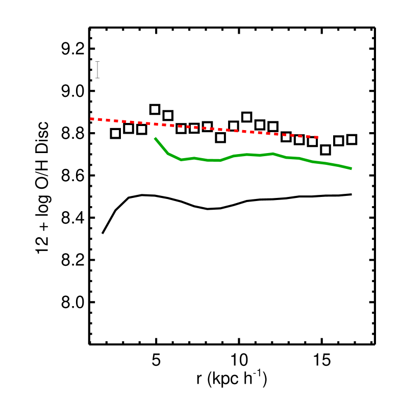
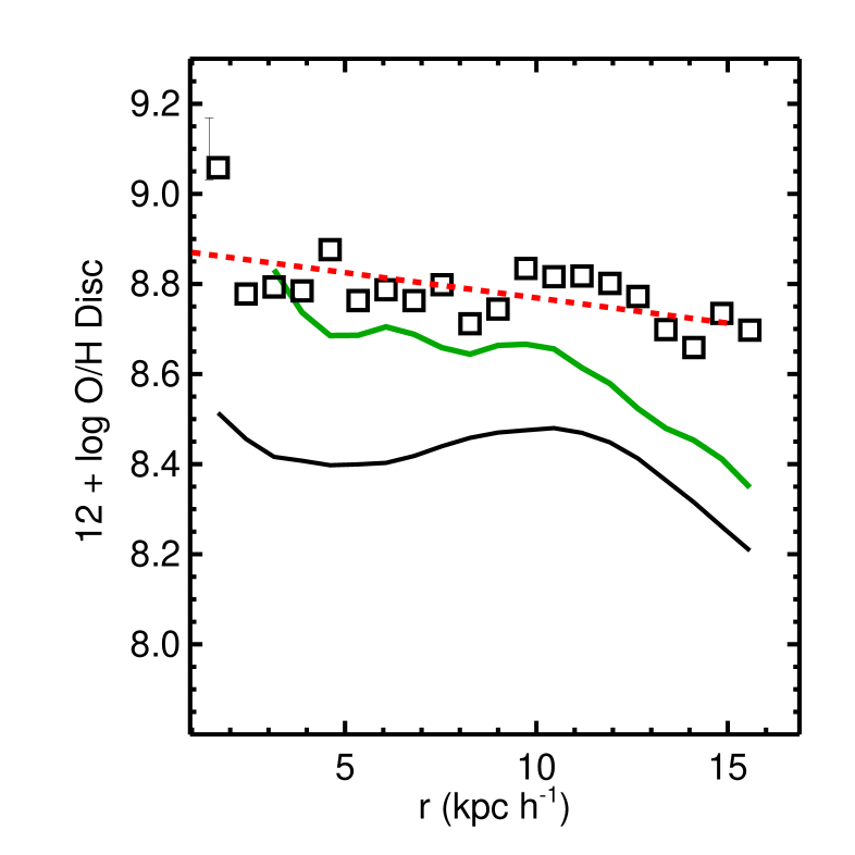
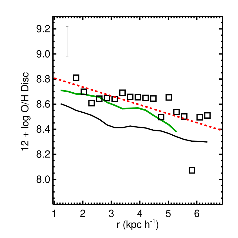
Figure 1: Oxygen abundance profiles determined for the gas component (open squares), the total stellar disc population (solid black lines) and the stars younger than 2 Gyrs in the simulated discs (green lines). The linear regressions to the gas abundance profiles are also included (red dashed lines). The abundance gradients correspond to three disc systems identified at $z\sim 0$ which exhibit negative abundance profiles. The total stellar mass of the galaxies (within $r_{\rm gal}$) are $6.68,4.19$ and $1.82\times 10^{10}$ M_⊙ (see the Section 3 for more details). The error bars represent the mean rms of the linear fits. This set of systems has been chosen only for illustration purposes.

3 Metallicity gradients and star formation of the disc galaxies

The abundance profiles for both the gas and the stars in the disc components are estimated by using the 12+logO/H ratios. We calculated the median abundance values for the gas phase, the total stellar populations and those stars with ages smaller than 2 Gyrs, an age limit usually assumed to select young stellar population by observers.

The median abundance profiles for the gas and stellar components are fitted with linear regressions (by a minimizing absolute deviation). For illustration purposes, in Fig. 1 we show the estimated gradients for three disc galaxies at $z\sim 0$, with total stellar masses (disc plus bulge stellar masses) between $\sim~{}2\times 10^{10}$ and $\sim~{}7\times 10^{10}$ M_⊙. As can be appreciated from this figure, the gas components show close to flat or negative abundance gradients and are enriched with respect to the median abundances of the whole stellar populations on the discs, as expected. For these galaxies the oxygen slopes are $-0.004$, $-0.008$ and $-0.05~{}{\rm dex~{}kpc^{-1}}$ (from the left panel to right one). These values of slopes are consistent with the best abundance determinations available, based on direct measurements of the gas electron temperature to derive O/H (e.g. Berg et al., 2015, and references therein.)

As we can see, the gas abundances are also slightly higher than those of the stars younger than 2 Gyrs. In most cases the trends defined by the young populations and the gas components are similar as expected, but the gas is also enriched by stars than 2 Gyrs. Hence, assuming this age interval to select stars to trace the current metallicity level of the ISM might lead to underestimations (and in some cases they might also show metallicity profiles with different slopes).

A similar analysis has been performed for simulated galaxies in the three redshift intervals. As a result, we have the gas-phase oxygen profiles of the disc components for galaxies with a variety of stellars masses at different stages of evolution. Hereafter we investigate the relationship between the oxygen gradients and the star formation activity as a function of their stellar mass by using the two subsamples defined in Section 2.1. The same stellar-mass limit was applied to the observational data. In the case of Ho et al. (2015) we use the mean values reported in their paper (table 1).

In Fig. 2 we plot the mean $M_{\rm star}$ and the mean oxygen slopes for the simulated gaseous disc and the observational data as a function of redshift. For comparison, the values of the corresponding individual simulated galaxies are also included. The media values and the errors are estimated by using a bootstrap technique (Table 1). These errors are the rms obtained with respect to the mean bootstrap values. As shown in this figure, at $z\sim 0$, the simulated oxygen slopes show a trend with the stellar mass which, albeit weak, is in agreement with the observational results reported by Ho et al. (2015). Note that the observational sample analysed by Ho et al. (2015) extends to lower stellar mass galaxies. The increase of the dispersion in the metallicity gradients for galaxies with smaller stellar masses is also in agreement with these observational results. At $z\sim 1$, the mean slopes are slightly more negative but a similar trend with the stellar mass is still present in the simulation. However, observations from Stott et al. (2014) and Queyrel et al. (2012) exhibit more positive and flat metallicity gradients, with no clear correlation signal. Note that the dispersion in the observations and simulated slopes are quite high (the Spearman rank correlation coefficients are $0.31(0.03)$ and $0.32(0.04)$ for $z\sim 0$ and $z\sim 1$, respectively.)

At higher redshifts, there are few measures of metallicity gradients and the available estimations show large dispersion (Yuan et al., 2011; Jones et al., 2013). Because of this, for the $z\sim 2$ interval, we plot the individual observed oxygen slopes instead of mean values as presented for the lower redshift ones. The Spearman rank correlation coefficient is $0.43(0.05)$. Although it is slightly larger than those measured at lower redshift, the statistical significance is lower. Metallicity gradients smaller than $-0.1~{}{\rm dex~{}kpc^{-1}}$ are mainly detected for galaxies with low stellar masses at $z>1$. In fact, galaxies with $M_{\rm star}>10^{10}M_{\odot}$ exhibit mean oxygen slopes which do not evolve significantly since $z\sim 2$, on average. The evolution of the slopes of the metallicity profiles is determined by simulated galaxies with $M_{\rm star}<10^{10}M_{\odot}$.

In order to assess the impact of disc galaxies with slopes more negative than $-0.1~{}{\rm dex~{}kpc^{-1}}$ on this correlation, we estimated the mean properties by excluding them. In this case, the mean values of the oxygen slopes of discs in the high stellar-mass subsample are weakly affected since they have small or null fractions of discs with very negative slopes (only at $z\sim 1,$, we detected a fraction of $19\%$ of the high stellar-mass discs to have such low metallicity gradients). Conversely, the results for galaxies in the low stellar-mass subsample are strongly modified. If disc galaxies with slopes smaller than $-0.1~{}{\rm dex~{}kpc^{-1}}$ are not considered, the mean slopes show either no correlation or a negative one, as it can be seen in Fig. 2 (open symbols). The fraction of discs with oxygen slopes lower than $-0.1~{}{\rm dex~{}kpc^{-1}}$ increases with increasing redshift for galaxies in this subsample ($21\%,40\%$ and $78\%$ for $z\sim 0,1,$ and 2, respectively).

We found no relation between the slopes of the oxygen profiles and the number of particles used to resolve the disc components (i.e. low number discs exhibit positive as well as negative slopes). And since we have used the same minimum limit in the number of particles at all analysed redshifts, numerical effects should affect similarly the three redshift subsamples. The metallicity gradients show no clear correlation with the gas fraction in the disc components.

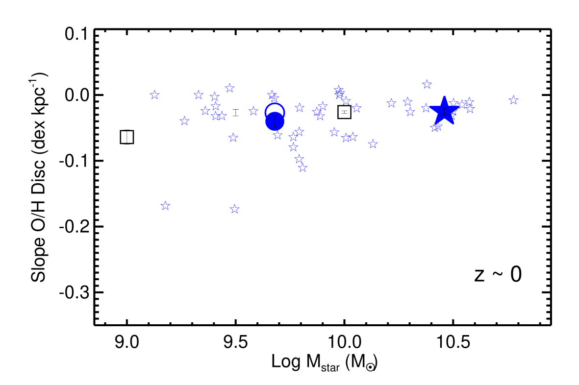
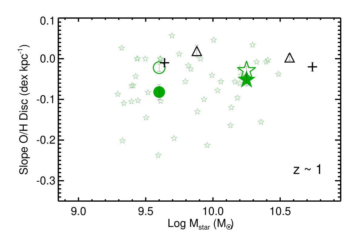
Figure 2: Mean slopes of gas-phase oxygen profiles as a function of total stellar mass of the simulated galaxies in the low (large filled circles) and high (large filled stars) stellar-mass subsamples, for $z\sim 0$ (blue symbols; upper panel), $z\sim 1$ (green symbols; middle panel) and $z\sim 2$ (magenta symbols; lower panel). Small open stars represent the values for individual simulated galaxies. The corresponding mean values obtained by excluding discs with gradients smaller than $-0.1~{}{\rm dex~{}kpc^{-1}}$ are also included for comparison (open symbols). Mean observed slopes for disc galaxies are also included: Ho et al. (2015, black squares) at $z\sim 0$ and Queyrel et al. (2012, black triangles) and Stott et al. (2014, black crosses) at $z\sim 1$ (see Section 3 for a detail description). At higher redshift, individual metallicity slopes reported by Jones et al. (2013, black diamonds) and Yuan et al. (2011, black open circle) have been included. Mean values and error bars were estimated by applying a bootstrap technique.

Table 1: Mean global properties of the simulated disc galaxies in the two defined stellar-mass subsamples as a function of redshift ($z$). The third column gives the number (N) of disc galaxies in the corresponding subsample. The three following columns provide: the mean gas-phase oxygen gradients (dex kpc^-1), the mean star formation rates ($M_{\odot}yr^{-1}$) and then mean specific star formation rates ($10^{-10}yr^{-1}$) for simulated discs galaxies. The last two columns show the parameters f_<-0.1 and f_>0 which represent the fractions of discs with metallicity slopes smaller than $-0.1~{}{\rm dex~{}kpc^{-1}}$ and with positive metallicity slopes, respectively.

Redshift	Log $M_{\rm stars}$	N	<Slope>	<SFR>	<sSFR>	f<-0.1	f>0
$z\sim 0$	$<10$	29	-0.041 $\pm$ 0.008	0.29 $\pm$ 0.05	0.7 $\pm$ 0.2	0.11	0.10
	$>10$	20	-0.025 $\pm$ 0.005	1.85 $\pm$ 0.41	0.6 $\pm$ 0.1	0.0	0.05
$z\sim 1$	$<10$	30	-0.080 $\pm$ 0.018	1.35 $\pm$ 0.29	4.04 $\pm$ 0.05	0.40	0.10
	$>10$	16	-0.052 $\pm$ 0.015	6.80 $\pm$ 0.91	3.67 $\pm$ 0.04	0.19	0.13
$z\sim 2$	$<10$	18	-0.18 $\pm$ 0.04	4.79 $\pm$ 0.63	10.90 $\pm$ 1.50	0.78	0.05
	$>10$	6	-0.03 $\pm$ 0.04	7.32 $\pm$ 0.87	5.90 $\pm$ 0.60	0.0	0.17

Table 2: Properties of the simulated disc galaxies. The stellar mass $M_{\rm stars}$ (second column), the star formation rate ($M_{\odot}yr^{-1}$; third column), the specific star formation rate ($yr^{-1}$, fourth column) and the gas-phase oxygen gradient (dex kpc^-1; fifth column) are given for ten simulated discs galaxies. The complete table is available online.

Redshift	Log $M_{\rm stars}$	SFR	sSFR	Slope
	10.98	7.91	8.30e-11	-0.005
	10.78	4.46	7.44e-11	-0.008
	10.56	2.76	7.31e-11	-0.021
	10.42	2.55	9.70e-11	-0.050
$z\sim 0$	10.57	2.62	6.99e-11	-0.011
	10.50	0.99	3.15e-11	-0.027
	10.43	0.84	3.14e-11	-0.048
	10.29	0.79	4.02e-11	-0.010
	10.38	0.85	3.57e-11	-0.020
	10.30	1.09	5.44e-11	-0.026

In order to understand the origin of both positive and very negative metallicity gradients, we first investigate if these galaxies follow the observed correlation between SFR and stellar mass (Karim et al., 2011) as a function of redshift (Daddi et al., 2007). In Fig.  3 we show the mean SFRs and the mean stellar masses of the simulated galaxies in the two stellar-mass subsamples as a function of redshift. The simulated relations are consistent with the observed one at $z\sim 0$. For higher redshifts, the simulated galaxies tend to have lower SFR than observations. However, we note that, on one hand, the range of stellar masses covered by the simulated galaxies at $z>0$ is smaller than the observed ones due our small simulated volume (note that the mean values for the high stellar-mass subsamples move to lower masses at higher redshifts). And that, on the other hand, observations tend to survey higher star formation systems for higher redshift (e.g. Mannucci et al., 2010; Salim et al., 2014) while in the simulations we are including galaxies of all types. Hence, the comparison should be taken with caution. Overall we find that at a given stellar mass, the star formation rate is larger for higher redshift.

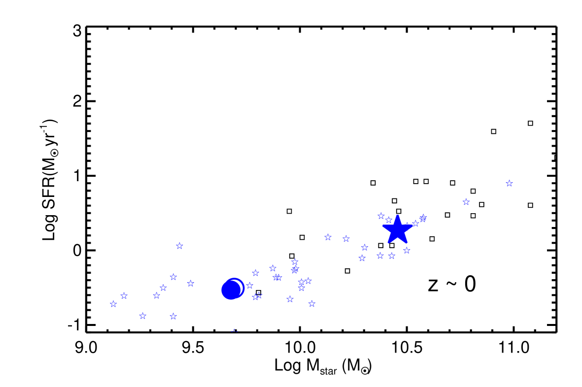
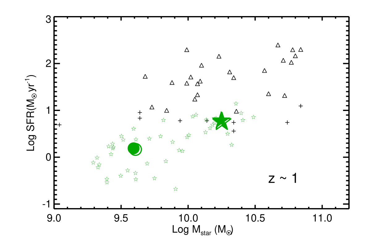
Figure 3: Mean star formation rate as a function of the mean stellar mass of simulated galaxies in the low (large filled circles) and high (large filled stars) stellar-mass subsamples for $z\sim 0$ (blue symbols; upper panel), $z\sim 1$ (green symbols; middle panel), $z\sim 2$ (magenta symbols; lower panel). Small open stars represent the values for individual simulated galaxies. Mean estimations obtained by excluding galaxies with slopes $<-0.1~{}{\rm dex~{}kpc^{-1}}$ are also included (open symbols). Most of them are superposed to the mean values from the whole sample. For comparison, we included the observational results from Rupke et al. (2010, black squares; $z\sim 0$), Queyrel et al. (2012, black triangles; $z\sim 1$), Stott et al. (2014, black, crosses; $z\sim 1$) and Jones et al. (2013, black, diamonds; $z\sim 2$). Mean values and error bars were estimated by applying a bootstrap technique.

3.1 A possible relation between the metallicity gradient and the sSFR?

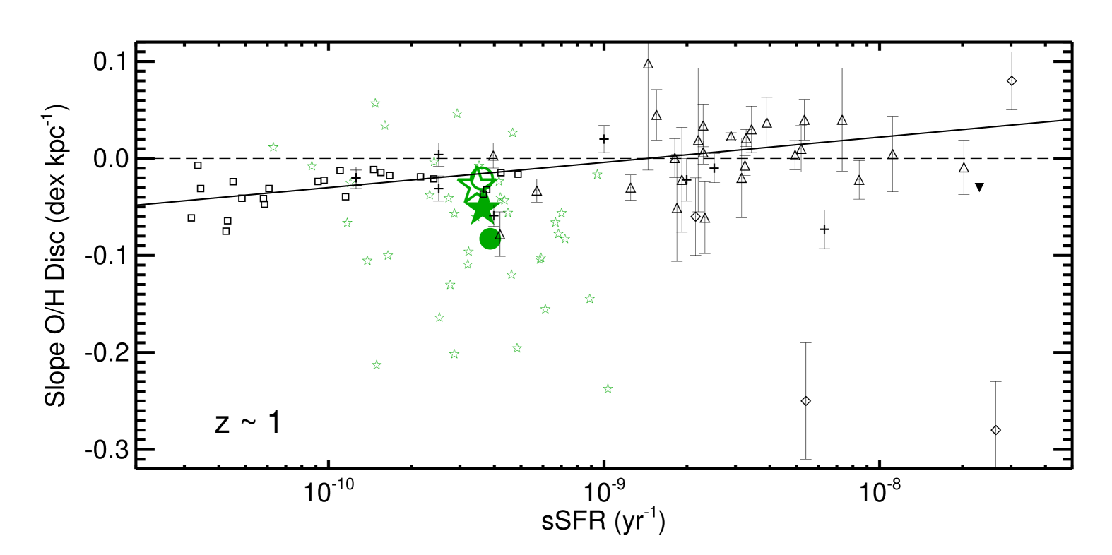
Figure 4: Mean slope of the gas-phased oxygen abundance profiles for the simulated ISMs as a function of the mean sSFR for galaxies for $z\sim 0$ (upper panel), $z\sim 1$ (middle panel) and $z\sim 2$ (lower panel) . Mean values have been estimated for galaxies in the low and high stellar-mass subsamples (large filled circles and stars, respectively). Small open stars represent the values for individual simulated galaxies (see Fig. 2 for color code). Estimations obtained by excluding oxygen slopes smaller than $-0.1~{}{\rm dex~{}kpc^{-1}}$ are also displayed (open circles and stars, respectively). For comparison we include the observational results from Rupke et al. (2010, black, open squares), Queyrel et al. (2012, black, open triangles), Jones et al. (2013, black, open rombus) Jones et al. (2015, black, inverted triangles), Stott et al. (2014, black, crosses) and the linear regression reported by Stott et al. (2014, solid line).

Recently Stott et al. (2014) reported evidences of a possible correlation between the slope of the oxygen gradients of disc galaxies and their sSFRs. These authors estimated these properties in their galaxy sample at $z\sim 1$ and included observations available in the literature for other redshifts. They proposed that mergers, and possibly secular evolution, could provide an explanation of the reported trends since they are known to be efficient mechanisms to drive gas inflows. If the galaxies have negative metallicity gradients, then these gas inflows will contribute with low metal-enriched gas, diluting the central abundances. In order to assess if such correlation is also present in our simulated galaxies, in Fig. 4 we plot the mean gas-phase metallicity slopes versus mean sSFR for the simulated galaxies in the two defined stellar-mass subsamples. Estimations for the the three defined redshift intervals have been included.

As can be seen from Fig. 4, at $z\sim 0$ simulated galaxies with low and high stellar-masses are consistent with the observed relation reported by Stott et al. (2014). In particular, massive galaxies have mean metallicity slopes and sSFRs which are consistent with the observed relation at all analysed redshift. For galaxies in the low stellar-mass subsample, the variation of the slopes and sSFRs with redshift are larger. These galaxies increase their sSFR for more than order of magnitude between $z\sim 0$ and $z\sim 2$ while their mean metallicity slopes decrease more strongly. As a consequence, they deviate form the observed relation. In the $z\sim 2$ interval, simulated galaxies show a wide spread in slopes going from positive to very negative ones. This is also true for the available observations.

We found that independently of their stellar masses, simulated galaxies have larger diversity of metallicity gradients with increasing redshift (Table 1). The fraction of galaxies with positive metallicity slopes increases with increasing redshift from $\sim 5$ percent at $z\sim 0$ to $\sim 17$ per cent at $z\sim 2$ for massive galaxies while for those with lower stellar masses, the fraction of positive metallicity slopes remains approximately constant with redshift ($10\%$). Conversely, the fraction of disc galaxies with metallicity slopes smaller than $-0.1~{}{\rm dex~{}kpc^{-1}}$ is larger in the low stellar-mass subsample and increases with redshift.

To evaluate the impact of the presence of the metallicity gradients smaller than $-0.1~{}{\rm dex~{}kpc^{-1}}$, we re-estimated the mean metallicity slopes and mean SFRs for the simulated galaxies excluding them. In this case, the mean simulated values for both the low and the high stellar-mass subsample are consistent with the Stott’s relation (note that the two observed points of Jones et al. (2013) had been included in Stott’s estimations).

Hence it would be important to confirm observationally the existence of such steep negative gradients at high redshift and their frequency in order to make a robust comparison with the simulations. These observations will provide important constrains for the sub-grid physics (principally the SN feedback model).

3.2 What are these systems?

In order to understand the origin of the very negative and the positive slopes, we explore the morphologies of the simulated galaxies and estimate the distances to the nearby galaxies. No major mergers are identified for these systems since $z<3$ but they experienced minor mergers and interactions (Pedrosa et al., 2014).

We found that gaseous discs with positive abundance gradients tend to exhibit morphological perturbations such as the presence of important central bars, clear ring structures in the discs or a very close companion, as can be seen from Fig. 5 where two examples are shown for illustration purposes. Regarding discs with very negative slopes, we find a more complex situation: some of them have close companions, others have central bars while the rest are consistent with having very concentrated mass distributions. Most of them shows either indications of low-metallicity accretion as the gas components have lower or similar median chemical abundances than the stars at a given radius, or of recent strong star formation activity in the central regions as the median gas abundances are much higher than those of the underlying stellar populations. In Fig. 6 we show two examples. We stress the fact that this is a qualitative description since there are not enough time-steps to follow the mergers and interactions in our cosmological run.

In order to shed light on this point, we resort to the analysis of the chemical evolution of galaxy pairs. These experiments showed that mergers and interactions could indeed trigger gas inflows which transport low-metallicity material into the central regions (Perez et al., 2006; Di Matteo et al., 2009b; Rich et al., 2012). In particular, Perez et al. (2011) followed the evolution of the metallicity gradients along the interactions using hydrodynamical simulations including chemical evolution. These authors reported the triggering of low-metallicity inflows which contribute to flatten the inner abundance profiles. These authors also showed clearly that as soon as this material reaches the central regions, the star formation conditions are generally satisfied and the gas is promptly transformed into stars. The new-born stars generate SNII which inject new $\alpha$-elements into the ISM, increasing the $\alpha$-abundances in the central regions and producing steeper negative oxygen gradients. These abundance profiles could become more positive again as galactic outflows from the inner regions transport enriched material outside the galaxy. Even more this enriched material could contribute to the outskirts of the discs if it cools down and is re-accreted by the main galaxy (see figure 7 in Perez et al., 2011). Hence, interactions could produce almost flat, positive slopes as well as negative ones, depending on the stage of the interactions, the gas availability and the characteristics of the disc systems (see figures 6 and 11 in Perez et al., 2011). Also the strength of the SN feedback could modulate the efficiency of these processes (e.g. Pilkington et al., 2012).

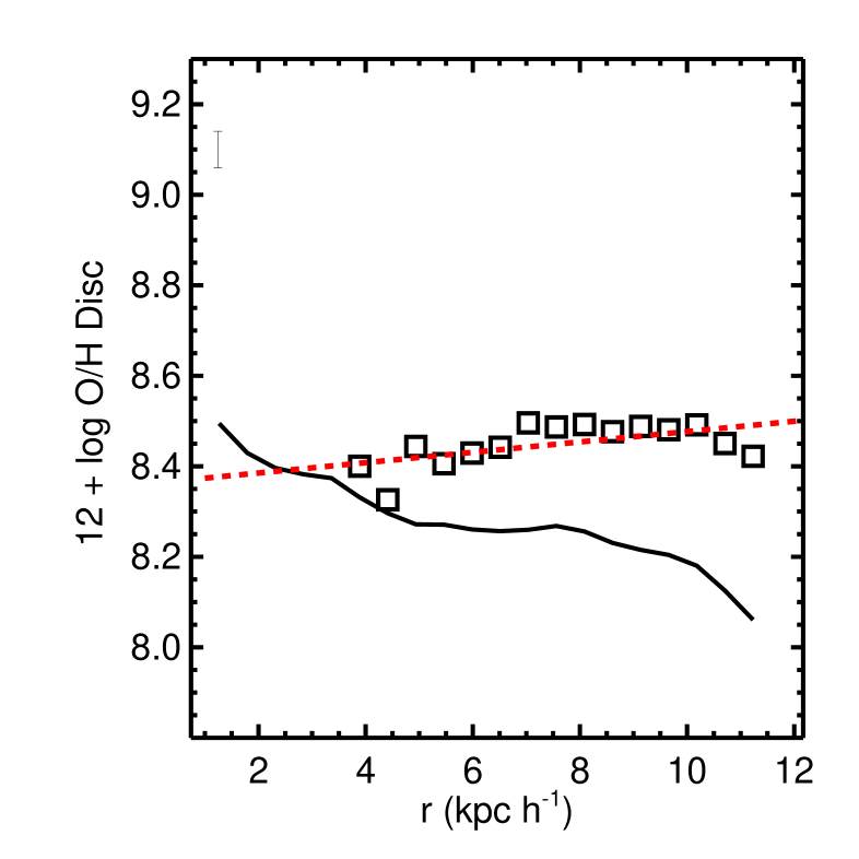
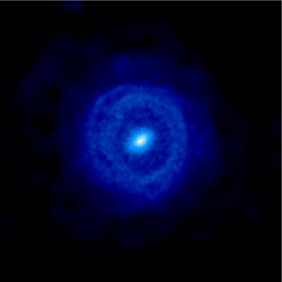
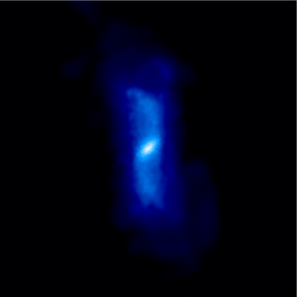
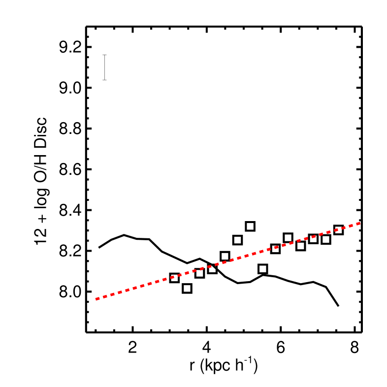
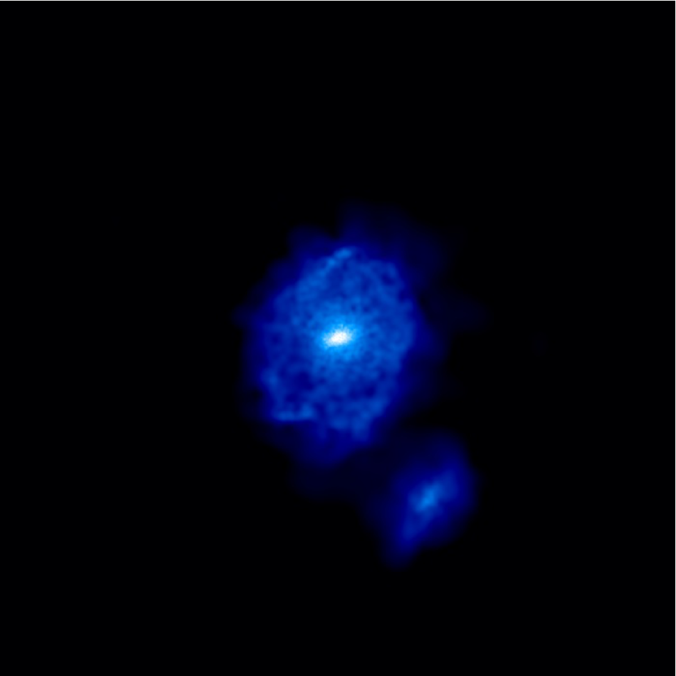
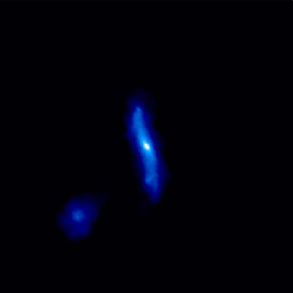
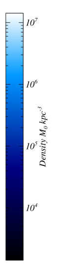
Figure 5: Mean $12+$log O/H profiles determined for the gas-phase disc components (open squares) and the stellar discs populations (black solid curves) in simulated galaxies which show positive gas abundance profiles. The linear regressions to the gas abundance profiles are also included (red lines). The error bars represent the mean rms of the linear fits. The density maps show the two projections of galaxies where we can appreciate the existence of a ring system (upper panel) and a close encounter (lower panel). Both simulated galaxies are at $z\sim 0.7$ and the images correspond to projected squares of 20 kpc a side.

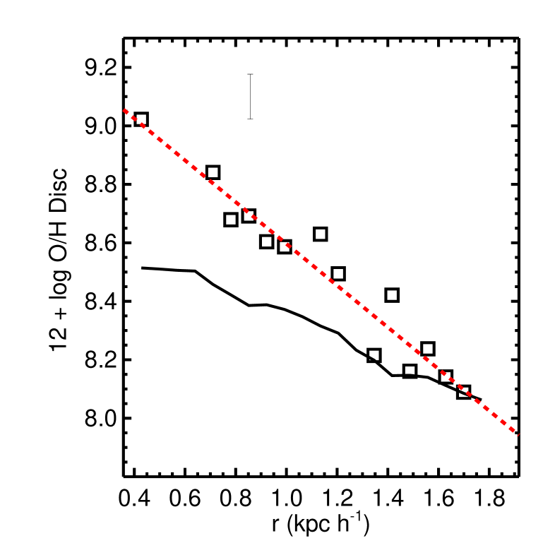
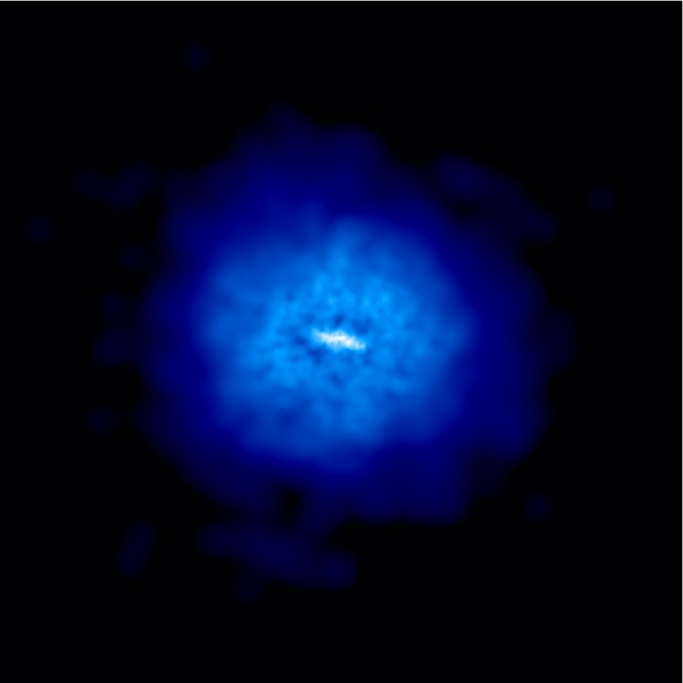
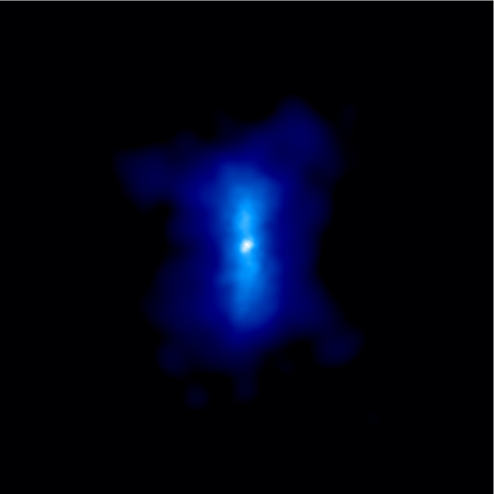
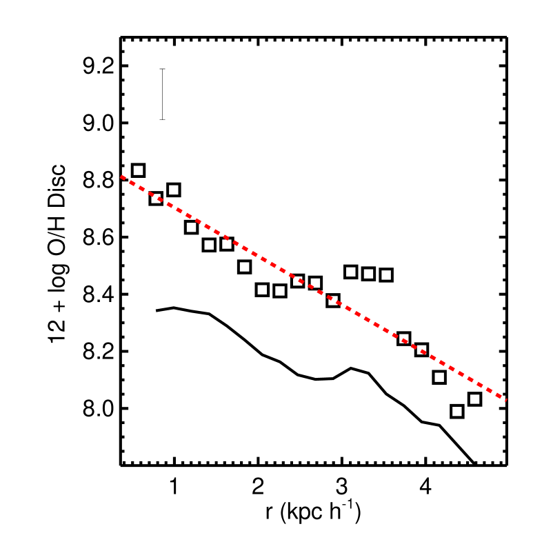
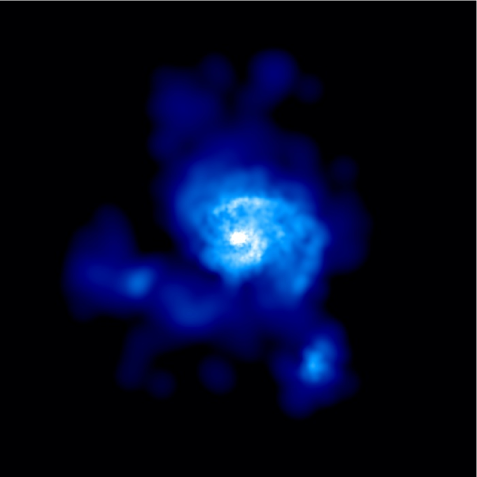
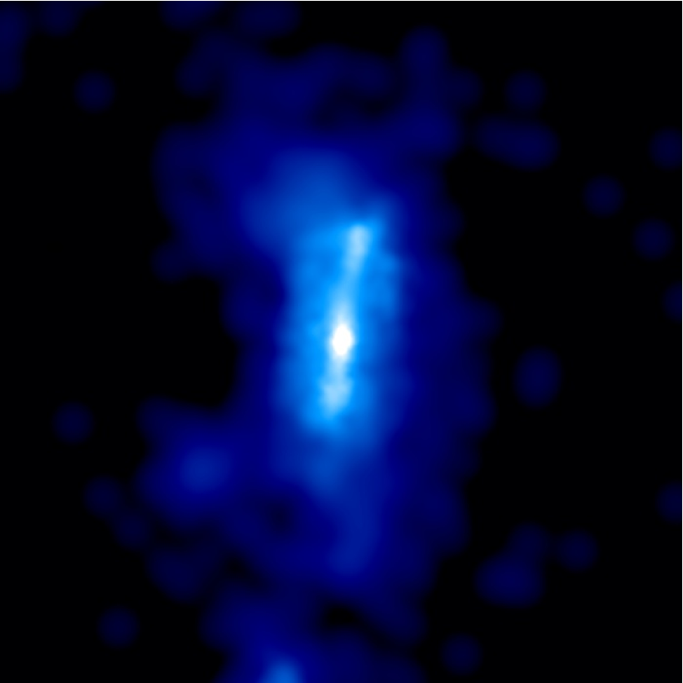
Figure 6: Mean $12+$log O/H profiles determined for the gas-phase disc components (open squares) and the stellar discs populations (black solid curves) in simulated galaxies which show very negative gas abundance profiles. The linear regressions to the gas abundance profiles are also included (red lines). The error bars represent the mean rms of the linear fits. The density maps show the two projections of galaxies where we can appreciate the existence of a concentrated bar (upper panel) and a close interaction (lower panel). Both galaxies are at $z\sim 2$ and the images correspond to projected squares of 10 kpc a side.

3.2.1 The effects of mergers

To explore the evolution of the metallicity gradient and the sSFR during a galaxy-galaxy interaction, we used the gas-rich major merger simulated by Perez et al. (2011). We choose this merger event since it provides a strong reaction to the effects of tidal fields during the interactions due to the high-gas content of the interacting systems. The simulation follows the evolution of a 1:1 major merger event with a gas fraction of $50\%$ in the disc. An important aspect to take into account is that the initial metallicity profiles of the interacting galaxies have been set ad hoc to have a slope of ${-0.07~{}\rm dex~{}kpc^{-1}}$ and a mean chemical abundance consistent with the mass-metallicity relation at $z\sim 2$ (Maiolino et al., 2008). Hence, this initial oxygen slope should be taken only as indicative. The relevant aspect to consider here is the change of the slope of the abundance profiles as a function of the sSFR, along the interaction.

In Fig. 7, we plot the sSFR versus the slope of the gas-phase oxygen profiles for the disc component in one of the interacting galaxies. These parameters evolve along the encounter in a complex way. To understand this evolutionary path, in Fig. 8 we show the metallicity gradient as a function of the relative distance between the mass centre and as a function of time. The time evolution of the sSFR is also included.

At the beginning the sSFR is high because of the high gas fraction in the galaxies and the slope of the metallicity gradient is close to $-0.07{~{}\rm dex~{}kpc^{-1}}$ as expected. As the systems approach each other, the slope of the metallicity gradients becomes less negative as gas inflows are driven inwards, carrying low-metallicity material (see also figures 8, 9 and 10 in Perez et al., 2011). The increase of the gas density produces new stars and hence, new chemical elements are injected into the ISM increasing the oxygen abundances. As a consequence, the slope of the metallicity gradient becomes negative again as can be seen from Fig. 8 (middle panel). After the apocentre and as galaxies approach each other again, positive slopes are detected. By this time, the galaxies are very close (less than $\sim 10$ kpc). Negative slopes are determined by the subsequent enrichment produced by the new stars. From this figure we can see that the behaviour is not smooth but the evolution of the metallicity gradients as a function of time shows a series of saw tooth as well as does the sSFR. These plots clearly illustrate how the increase of the sSFR can be related to the flattening of the metallicity gradients and how they become more negative as new stars inject massively $\alpha$-elements in the central regions. This can also be correlated with an increase of the [O/Fe] ratio as reported by Perez et al. (2011, figure 8d).

If galaxies formed consistently within a $\Lambda$-CDM cosmology, mergers and interactions would be ubiquitous, mainly in the high-redshift Universe. These violent events could cause different perturbations in the metallicity gradients, providing a range of situations which are not covered by the equal-mass, gas-rich merger investigated in this Section. However, this simulation illustrates clearly a possible evolutionary path for the metallicity gradients during interactions and accounts for the negative and the positive slopes found in the discs galaxies simulated in a cosmological framework.

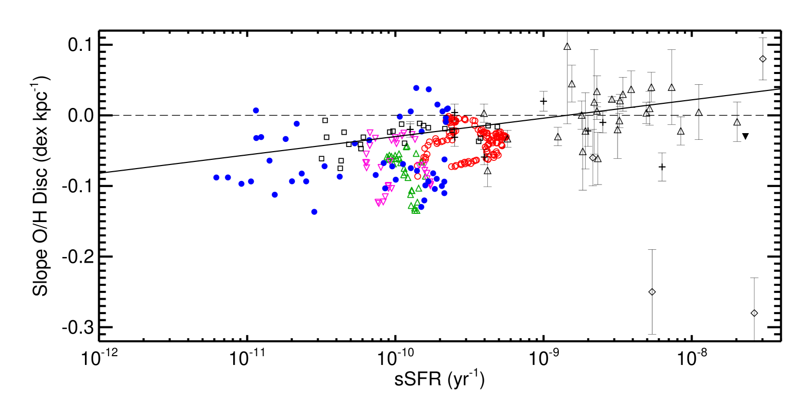
Figure 7: Slope of the gas-phase oxygen profiles as a function of the sSFR for a galaxy in a gas-rich major merger. We denote the periods before the pericentre (red open circles), between the pericentre and apocentre (green triangles), between the apocentre and the second pericentre (magenta inverted triangles) and after the second pericentre (blue filled circles). For comparison we include the observational results from Rupke et al. (2010, black, open squares), Queyrel et al. (2012, black, open triangles), Jones et al. (2013, black, open rombus) Jones et al. (2015, black, inverted triangles), Stott et al. (2014, black, crosses) and the linear regression reported by Stott et al. (2014, solid line). The galaxy starts with an ad hoc metallicity slope of ${-0.07~{}\rm dex~{}kpc^{-1}}$. See Fig. 8 and Section 3.2.1 for details.

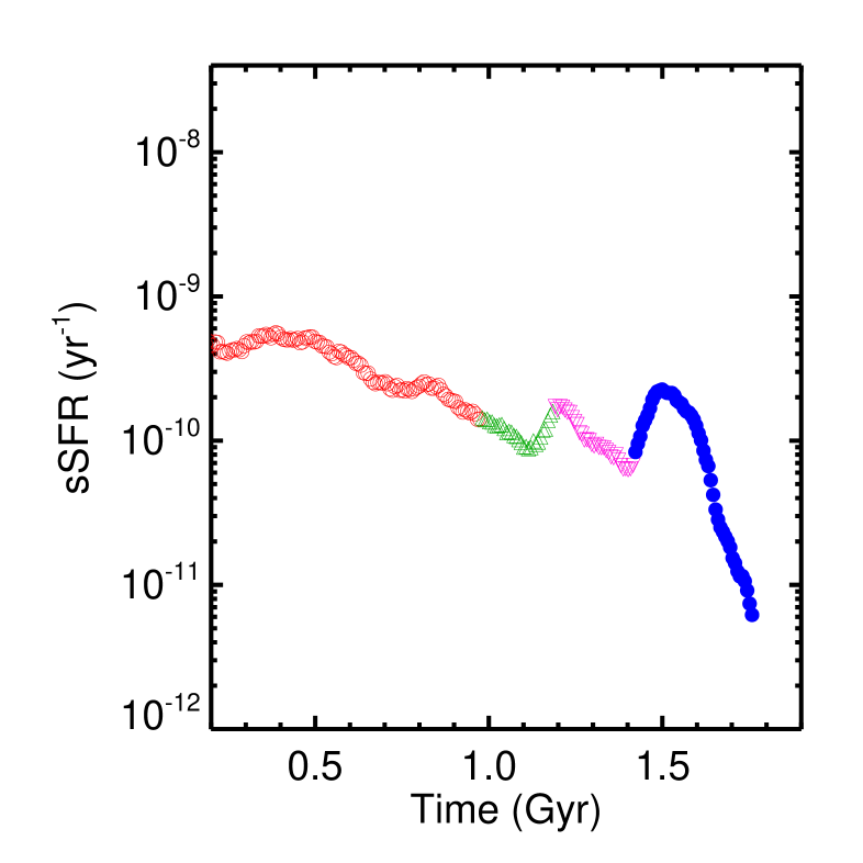
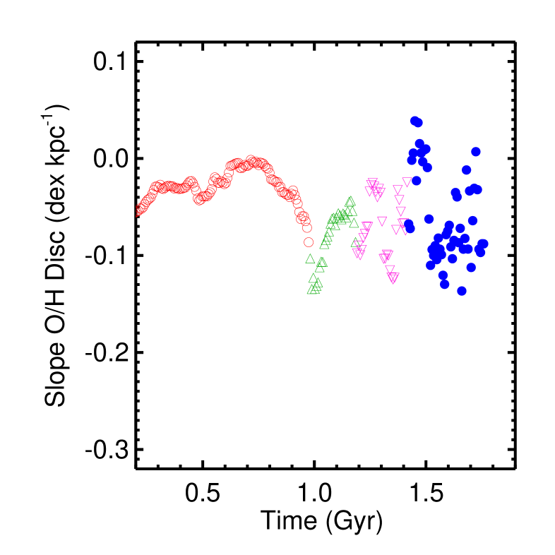
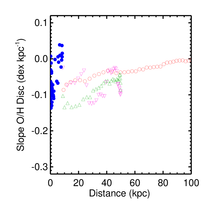
Figure 8: Time evolution of sSFR (left panel) and the gas-phase oxygen gradients (middle panel). The evolution of the gradients as a function of distance between the mass centres are also included (right panel). Key periods of the encounter are shown in different colours (see Fig. 7 for colour-code).

4 Conclusions

We studied the chemical abundance profiles of the gas-phase disc components in relation to the star formation activity of the galaxies simulated in a hierarchical universe. For this purpose, we analysed a set of galaxies extracted from a cosmological simulation consistent with a $\Lambda$CDM scenario, performed using a hydrodynamical code which includes energy and chemical feedback by SNII and SNIa. We performed the analysis as a function of stellar mass in the range $[10^{9}-10^{11}]$ M$\odot$ by adopting a stellar-mass limit of $M_{\rm star}=10^{10}$M$\odot$. The global SFR of the simulated galaxies as a function of stellar mass are consistent with observational values.

Our main results can be summarized as follows:

• At $z\sim 0$ the gas-phase oxygen slopes of the simulated discs show a trend with the stellar mass in agreement with observations. Galaxies with lower stellar masses have metallicity gradients which exhibit larger dispersion than those measured in galaxies with larger masses, in agreement with observations results (Ho et al., 2015).

  Massive galaxies show very weak evolution of their oxygen gradients with redshift (i.e. the change in the mean oxygen slopes between $z\sim 0$ and $z\sim 2$ is within the bootstrap dispersion). Conversely, galaxies with lower stellar masses show more significant changes of the metallicity gradients with redshift, so that they get steeper with increasing redshift. At $z\sim 1$ our simulated discs exhibit slighlty steeper negative metallicity slopes than those reported by current observations. At $z\sim 2$ there are few available observations which have diverse metallicity gradients. At these high redshifts, the simulated metallicity slopes also show a noticeable scatter for galaxies with low stellar masses, but the mean value is dominated by the negative gradients.

  The fraction of gaseous discs with slopes smaller than $-0.1~{}{\rm dex~{}kpc^{-1}}$ in galaxies with low stellar-masses varies from 0.10 at $z\sim 0$ to 0.78 $z\sim 2$. In the high stellar-mass subsample the fraction is small or null. Conversely, the fraction of disc galaxies with positive slopes is found to be approximately constant for galaxies with low stellar masses ($\sim 0.10$ on average) but to increase with increasing redshift for the galaxies with higher stellar masses (from $\sim 0.05$ at $z\sim 0$ to $\sim 0.17$ at $z\sim 2$).

• At $z\sim 0$, galaxies with both low and high stellar masses have mean metallicity slopes and sSFR consistent with the relation reported by Stott et al. (2014). Galaxies with high stellar masses have values which are consistent with the Stott’s relation in the three redshift interval analysed. However, galaxies with the lower masses deviate from the observed relation for higher redshift as the results of the increasing contribution of gaseous discs with metallicity slopes smaller than $-0.1~{}{\rm dex~{}kpc^{-1}}$. If disc galaxies with such negative slopes are not included, then the mean values for both low and high stellar-mass galaxies are consistent with observed relations. We note that Stott et al. (2014) did not include the steeper negative slopes reported by Jones et al. (2013). However, in this case the correlation between the slope of the oxygen gradients and stellar mass is lost. At $z\sim 0$, this is in open disagreement with observational results, suggesting that a fraction of steep negative slopes should be present for low stellar-mass galaxies (Ho et al., 2015). At higher redshift, a large observational data sample with more precise metallicity estimations is required in order to study the presence and frequency of very negative and positive slopes as a function of stellar mass.

• We explore the morphology and surrounding media of our simulated galaxies finding that galaxies with positive and very negative metallicity slopes have disturbed morphologies and close neighbours. However, due to the low-number sample, it is not possible to derive a stastically robust trend. However, since they all have a system of surrounding satellites (of different masses) the probability of interactions/mergers is expected to be high. The analysis of a simulated merger of two gas-rich equal-mass galaxies yields that both negative and positive metallicity gradients might be produced during different stages of evolution of the encounter. It remains to be investigated if internal instabilities (such as secular evolution) could also lead to a similar relation between the sSFR and the metallicity gradients and if the predicted relation can be distinguish from that of galaxies with mergers and interactions.

Our results provide an interpretation to the observed relation reported by Stott et al. (2014). However, a significant number of negative slopes, such as those reported by Jones et al. (2013), are detected for simulated galaxies with low stellar masses. The presence of such metallicity profiles needs to be confirmed by larger observed galaxy samples. In such case the location of a disc galaxy on this relation might tell us about its current evolutionary status as well as its past history. Otherwise, it might suggest that our simulations are overpredicted them, and hence our subgrid physics should be accordingly revised. As shown in previous works, the characteristics of the subgrid physics have an important impact on the chemodynamical properties of galaxies (e.g. Pilkington et al., 2012; Gibson et al., 2013; Snaith et al., 2013). Hence the confrontation of the chemical properties of galaxies with observation is indeed a powerful tool to set constrains on galaxy formation models.

References

- Amorín et al. (2012) Amorín R., Vílchez J. M., Hägele G. F., Firpo V., Pérez-Montero E., Papaderos P., 2012, ApJL, 754, L22
- Amorín et al. (2010) Amorín R. O., Pérez-Montero E., Vílchez J. M., 2010, ApJL, 715, L128
- Aumer et al. (2013) Aumer M., White S. D. M., Naab T., Scannapieco C., 2013, MNRAS, 434, 3142
- Barnes & Hernquist (1996) Barnes J. E., Hernquist L., 1996, ApJ, 471, 115
- Berg et al. (2015) Berg D. A., Skillman E. D., Croxall K. V., Pogge R. W., Moustakas J., Johnson-Groh M., 2015, ApJ, 806, 16
- Bland-Hawthorn & Freeman (2003) Bland-Hawthorn J., Freeman K. C., 2003, in E. Perez, R. M. Gonzalez Delgado, & G. Tenorio-Tagle ed., Star Formation Through Time Vol. 297 of Astronomical Society of the Pacific Conference Series, Unravelling the Epoch of Dissipation. pp 457–+
- Calura et al. (2012) Calura F., Gibson B. K., Michel-Dansac L., Stinson G. S., Cignoni M., Dotter A., Pilkington K., House E. L., Brook C. B., Few C. G., Bailin J., Couchman H. M. P., Wadsley J., 2012, MNRAS, 427, 1401
- Chiappini et al. (1997) Chiappini C., Matteucci F., Gratton R., 1997, ApJ, 477, 765
- Chiappini et al. (2001) Chiappini C., Matteucci F., Romano D., 2001, ApJ, 554, 1044
- Cora (2006) Cora S. A., 2006, MNRAS, 368, 1540
- Daddi et al. (2007) Daddi E., Dickinson M., Morrison G., Chary R., Cimatti A., Elbaz D., Frayer D., Renzini A., Pope A., Alexander D. M., Bauer F. E., Giavalisco M., Huynh M., Kurk J., Mignoli M., 2007, ApJ, 670, 156
- De Lucia et al. (2014) De Lucia G., Tornatore L., Frenk C. S., Helmi A., Navarro J. F., White S. D. M., 2014, MNRAS, 445, 970
- De Rossi et al. (2013) De Rossi M. E., Avila-Reese V., Tissera P. B., González-Samaniego A., Pedrosa S. E., 2013, MNRAS, 435, 2736
- Di Matteo et al. (2009a) Di Matteo P., Pipino A., Lehnert M. D., Combes F., Semelin B., 2009a, AA, 499, 427
- Di Matteo et al. (2009b) Di Matteo P., Pipino A., Lehnert M. D., Combes F., Semelin B., 2009b, A&A, 499, 427
- Ellison et al. (2008) Ellison S. L., Patton D. R., Simard L., McConnachie A. W., 2008, AJ, 135, 1877
- Fakhouri et al. (2010) Fakhouri O., Ma C.-P., Boylan-Kolchin M., 2010, MNRAS, 406, 2267
- Gibson et al. (2013) Gibson B. K., Pilkington K., Brook C. B., Stinson G. S., Bailin J., 2013, A&A, 554, A47
- Ho et al. (2015) Ho I.-T., Kudritzki R.-P., Kewley L. J., Zahid H. J., Dopita M. A., Bresolin F., Rupke D. S. N., 2015, MNRAS, 448, 2030
- Iwamoto et al. (1999) Iwamoto K., Brachwitz F., Nomoto K., Kishimoto N., Umeda H., Hix W. R., Thielemann F.-K., 1999, ApJS, 125, 439
- Jimenez et al. (2014) Jimenez N., Tissera P. B., Matteucci F., 2014, Memorie della Societa Astronomica Italiana, 85, 325
- Jimenez et al. (2015) Jimenez N., Tissera P. B., Matteucci F., 2015, ApJ, 810, 137
- Jones et al. (2013) Jones T., Ellis R. S., Richard J., Jullo E., 2013, ApJ, 765, 48
- Jones et al. (2015) Jones T., Wang X., Schmidt K. B., Treu T., Brammer G. B., Bradač M., Dressler A., Henry A. L., Malkan M. A., Pentericci L., Trenti M., 2015, AJ, 149, 107
- Karim et al. (2011) Karim A., Schinnerer E., Martínez-Sansigre A., Sargent M. T., van der Wel A., Rix H.-W., Ilbert O., Smolčić V., Carilli C., Pannella M., Koekemoer A. M., Bell E. F., Salvato M., 2011, ApJ, 730, 61
- Kewley & Ellison (2008) Kewley L. J., Ellison S. L., 2008, ApJ, 681, 1183
- Kewley et al. (2006) Kewley L. J., Geller M. J., Barton E. J., 2006, AJ, 131, 2004
- Kewley et al. (2010) Kewley L. J., Rupke D., Zahid H. J., Geller M. J., Barton E. J., 2010, ApJL, 721, L48
- Kobayashi et al. (2007) Kobayashi C., Springel V., White S. D. M., 2007, MNRAS, 376, 1465
- Maiolino et al. (2008) Maiolino R., Nagao T., Grazian A., Cocchia F., Marconi A., Mannucci F., Cimatti A., Pipino A. e. a., 2008, A&A, 488, 463
- Mannucci et al. (2010) Mannucci F., Cresci G., Maiolino R., Marconi A., Gnerucci A., 2010, MNRAS, 408, 2115
- Marino et al. (2013) Marino R. A., Rosales-Ortega F. F., Sánchez S. F., Gil de Paz A., Vílchez J., Miralles-Caballero D., Kehrig C., Pérez-Montero E., Stanishev V., Califa Team 2013, A&A, 559, A114
- Mast et al. (2014) Mast D., Rosales-Ortega F. F., Sánchez S. F., Vílchez J. M., Iglesias-Paramo J., Walcher C. J., Husemann B., Márquez I., Marino R. A., Kennicutt R. C., et al. 2014, A&A, 561, A129
- Matteucci & Greggio (1986) Matteucci F., Greggio L., 1986, AA, 154, 279
- Michel-Dansac et al. (2008) Michel-Dansac L., Lambas D. G., Alonso M. S., Tissera P., 2008, MNRAS, 386, L82
- Mollá & Ferrini (1995) Mollá M., Ferrini F., 1995, ApJ, 454, 726
- Mollá et al. (1997) Mollá M., Ferrini F., Díaz A. I., 1997, ApJ, 475, 519
- Mosconi et al. (2001) Mosconi M. B., Tissera P. B., Lambas D. G., Cora S. A., 2001, MNRAS, 325, 34
- Pedrosa & Tissera (2015a) Pedrosa S., Tissera P., 2015a, ArXiv e-prints
- Pedrosa & Tissera (2015b) Pedrosa S., Tissera P., 2015b, A&A, accepted
- Pedrosa et al. (2014) Pedrosa S. E., Tissera P. B., De Rossi M. E., 2014, A&A, 567, A47
- Perez et al. (2011) Perez J., Michel-Dansac L., Tissera P. B., 2011, MNRAS, 417, 580
- Perez et al. (2006) Perez M. J., Tissera P. B., Scannapieco C., Lambas D. G., de Rossi M. E., 2006, AA, 459, 361
- Pilkington et al. (2012) Pilkington K., Gibson B. K., Brook C. B., Calura F., Stinson G. S., Thacker R. J., Michel-Dansac L., Bailin J., Couchman H. M. P., Wadsley J., Quinn T. R., Maccio A., 2012, MNRAS, 425, 969
- Queyrel et al. (2012) Queyrel J., Contini T., Kissler-Patig M., Epinat B., Amram P., Garilli B., Le Fèvre O., Moultaka J., Paioro L., Tasca L., Tresse L., Vergani D., López-Sanjuan C., Perez-Montero E., 2012, A&A, 539, A93
- Rich et al. (2012) Rich J. A., Torrey P., Kewley L. J., Dopita M. A., Rupke D. S. N., 2012, ApJ, 753, 5
- Rupke et al. (2010) Rupke D. S. N., Kewley L. J., Chien L., 2010, ArXiv e-prints
- Salim et al. (2014) Salim S., Lee J. C., Ly C., Brinchmann J., Davé R., Dickinson M., Salzer J. J., Charlot S., 2014, ApJ, 797, 126
- Sánchez et al. (2014) Sánchez S. F., Rosales-Ortega F. F., Iglesias-Páramo J., Mollá M., Barrera-Ballesteros J., Marino R. A., Pérez E., Sánchez-Blazquez P., González Delgado R. e. a., 2014, A&A, 563, A49
- Sanchez et al. (2013) Sanchez S. F., Rosales-Ortega F. F., Jungwiert B., Iglesias-Paramo1 J., Vilchez J. M., Marino R. A., Walcher C. J., Husemann B., Mast D., The CALIFA collaboration 2013, ArXiv e-prints
- Sánchez-Blázquez et al. (2014) Sánchez-Blázquez P., Rosales-Ortega F. F., Méndez-Abreu J., Pérez I., Sánchez S. F., Zibetti S., Aguerri J. A. L., Bland-Hawthorn J., Catalán-Torrecilla C. e. a., 2014, A&A, 570, A6
- Scannapieco et al. (2005) Scannapieco C., Tissera P. B., White S. D. M., Springel V., 2005, MNRAS, 364, 552
- Scannapieco et al. (2006) Scannapieco C., Tissera P. B., White S. D. M., Springel V., 2006, MNRAS, 371, 1125
- Scannapieco et al. (2008) Scannapieco C., Tissera P. B., White S. D. M., Springel V., 2008, MNRAS, 389, 1137
- Schaye et al. (2015) Schaye J., Crain R. A., Bower R. G., Furlong M., Schaller M., Theuns T., Dalla Vecchia C., Frenk C. S., McCarthy I. G. e. a., 2015, MNRAS, 446, 521
- Snaith et al. (2013) Snaith O. N., Tissera P. B., Pedrosa S., de Rossi M. E., Vílchez J. M., 2013, Asociacion Argentina de Astronomia La Plata Argentina Book Series, 4, 129
- Springel (2005) Springel V., 2005, MNRAS, 364, 1105
- Springel et al. (2001) Springel V., Yoshida N., White S. D. M., 2001, New Astronomy, 6, 79
- Stott et al. (2014) Stott J. P., Sobral D., Swinbank A. M., Smail I., Bower R., Best P. N., Sharples R. M., Geach J. E., Matthee J., 2014, MNRAS, 443, 2695
- Swinbank et al. (2012) Swinbank A. M., Sobral D., Smail I., Geach J. E., Best P. N., McCarthy I. G., Crain R. A., Theuns T., 2012, MNRAS, 426, 935
- Tissera (2000) Tissera P. B., 2000, ApJ, 534, 636
- Tissera et al. (2013) Tissera P. B., Scannapieco C., Beers T. C., Carollo D., 2013, MNRAS, 432, 3391
- Tissera et al. (2012) Tissera P. B., White S. D. M., Scannapieco C., 2012, MNRAS, 420, 255
- Wiersma et al. (2009) Wiersma R. P. C., Schaye J., Theuns T., Dalla Vecchia C., Tornatore L., 2009, MNRAS, 399, 574
- Woosley & Weaver (1995) Woosley S. E., Weaver T. A., 1995, ApJS, 101, 181
- Yuan et al. (2011) Yuan T.-T., Kewley L. J., Swinbank A. M., Richard J., Livermore R. C., 2011, ApJL, 732, L14