Flavour changing and conserving processes
Higher order hadronic and leptonic contributions to the muon
Abstract
In this contribution we discuss next-to-next-to-leading order hadronic and four-loop QED contributions to the anomalous magnetic moment of the muon.
1 Introduction
The anomalous magnetic moment of the muon, , is among the most precise measured quantities in particle physics. It is measured to a precision of 0.54 parts per million which matches the precision of the Standard Model theory prediction Bennett:2006fi ; Roberts:2010cj . However, since many years one observes a discrepancy of about three to four standard deviations which survives persistent all improvements. This concerns both the experimental data and theoretical calculations entering the prediction.
Currently a new experiment is built at FERMILAB with the aim to increase the accuracy of the measured value by about a factor four Carey:2009zzb ; Herzog_fccp15 . In the upcoming years also improvements on the theory side can be expected. On the one hand this is connected to improved measurements of at low energies (see, e.g., Refs. Aubert:2009ad ; Ambrosino:2010bv ; Eidelman_fccp15 ). On the other hand it can be expected that within the next few years results from lattice simulations become available both for the hadronic vacuum polarization and hadronic light-by-light contributions (see, e.g., Refs. DellaMorte:2011aa ; Burger:2013jya ; Blum:2014oka ; Blum:2015gfa ; Lehner_fccp15 ).
The by far dominant numerical contribution to originates from QED corrections which are known to five-loop order Aoyama:2012wk . Note, however, that the four- and the five-loop corrections have only been computed by a single group.111Partial four-loop corrections have been obtained in Refs. Laporta:1993ds ; Baikov:1995ui ; Aguilar:2008qj ; Lee:2013sx ; Baikov:2012rr ; Baikov:2013ula . For this reason we have recently started to systematically check the four-loop results of Aoyama:2012wk . In Ref. Lee:2013sx analytic results for the gauge-invariant subsets with two or three closed electron loops have been obtained neglecting power corrections of the form . All contributions involving a lepton have been computed in Ref. Kurz:2013exa . After including three (analytic) expansion terms in a better precision has been obtained than in the numerical approach of Ref. Aoyama:2012wk . The numerically most important QED contributions at four-loop level arise from light-by-light-type diagrams (i.e. the external photon does not couple to the external muon line) containing a closed electron loop. This well-defined subset has been considered in Ref. Kurz:2015bia where an asymptotic expansion for has been performed to compute four expansion terms.
We adopt the notation from Ref. Aoyama:2012wk and parametrize the anomalous magnetic moment in the form
| (1) |
where the four-loop contribution can be written as
| (2) | |||||
contains only contributions from photons and muons, and involve closed electron or tau loops, and each Feynman diagram which contributes to contains all three lepton flavours simultaneously. In Sections 2 and 3 we describe the calculation of the light-by-light type QED contribution to (see also Kurz:2015bia ) and the computation of (see also Kurz:2013exa ), respectively. Afterwards we summarize in Section 4 the computation of the next-to-next-to-leading order (NNLO) hadronic vacuum polarization contribution published in Ref. Kurz:2014wya . A brief summary and an outlook is given in Section 5.
2 Four-loop electron contribution
The numerically most important contribution to originates from diagrams involving a closed electron loop (denoted by in Eq. (2). This contribution contains a gauge invariant subset where the external photon does not couple to the external muon line but to a closed fermion loop, the so-called leptonic light-by-light-type diagrams. Due to Furry’s theorem such diagrams do not contribute at two but only start at three loops where four photons can be attached to the closed fermion loop. Here we discuss the four-loop result which can be sub-divided into three gauge invariant and finite contributions which we denote by IV(a), IV(d) and IV(c). Sample Feynman diagrams are shown in Fig. 1. Case IV(a) can be further subdivided according to the flavour of the leptons in the closed fermion loops. The contribution with two electron loops is denoted by IV(a0), the one with one muon and one electron loop and the coupling of the external photon to the electron by IV(a1), and the remaining one with one muon and one electron loop by IV(a2). We do not consider the case with two muon loops since this contribution is part of .


IV(a) IV(b) IV(c)
The light-by-light-type diagrams are numerically dominant and provide about 95% of the four-loop electron loop contribution. The main reason for this are terms which are even present in the limit . In fact, IV(a0) even has quadratic logarithms which makes this part the most important one.
Our calculation is based on an asymptotic expansion Beneke:1997zp ; Smirnov:2013 for which is implemented with the help of asy Pak:2010pt ; Jantzen:2012mw and in-house Mathematica programs. Similar to the hard mass procedure applied in Section 3 we obtain a factorization of the original two-scale integrals into products of one-scale integrals. The latter are either vacuum or on-shell integrals or integrals containing eikonal propagators of the form (see Ref. Kurz:2015bia for more details). For each integral class we perform a reduction to master integrals and obtain analytic results expressed as a linear combination of about 150 so-called master integrals. About 50% of them we know analytically or to high numerical precision. The remaining ones are computed with the help of the package FIESTA Smirnov:2013eza which is the source of the numerical uncertainty in our final result. We would like to stress that in our approach a systematic improvement is possible if it is required to improve the accuracy.
| Kurz:2015bia | Kinoshita:2004wi ; Aoyama:2012wk | |
|---|---|---|
| IV(a0) | ||
| IV(a1) | ||
| IV(a2) | ||
| IV(a) | ||
| IV(b) | ||
| IV(c) |
For all five cases we compute terms up to order (i.e. four expansion terms) and check that the cubic corrections only provide a negligible contribution. Our final results can be found in Tab. 1 where we compare to the findings of Refs. Kinoshita:2004wi ; Aoyama:2012wk . Note that results for IV(a0) have also been obtained in Refs. Calmet:1975tw ; Chlouber:1977dr , though with significantly larger uncertainty. In all cases good agreement is found with Kinoshita:2004wi ; Aoyama:2012wk . Although our numerical uncertainty, which amounts to approximately , is larger, the final result is nevertheless sufficiently accurate as can be seen by the comparison to the difference between the experimental result and theory prediction which is given by
| (3) |
This result is taken from Ref. Aoyama:2012wk . Note that the uncertainty in Eq. (3) receives approximately the same amount from experiment and theory. Even after a projected reduction of the uncertainty by a factor four both in and our numerical precision is a factor ten below the uncertainty of the difference.
3 Four-loop tau lepton contribution
In this section we discuss the gauge invariant and finite subset of Feynman diagrams involving a closed heavy tau lepton loop. In the limit of infinitely heavy this contribution has to vanish. Thus has a parametric dependence which is of order . Note, that and thus one can expect that the four-loop tau lepton contribution is of the same order as the universal five-loop result Aoyama:2012wk .
We compute this contribution by applying an asymptotic expansion in the limit . This is realized with the help of the program exp Harlander:1997zb ; Seidensticker:1999bb which is written in C++. As a result the two-scale four-loop integrals factorize into one-scale vacuum () and on-shell () integrals. Both integral classes are well studied in the literature (for references see Kurz:2013exa ). This concerns both the reduction to master integrals and the analytic evaluation of the latter.
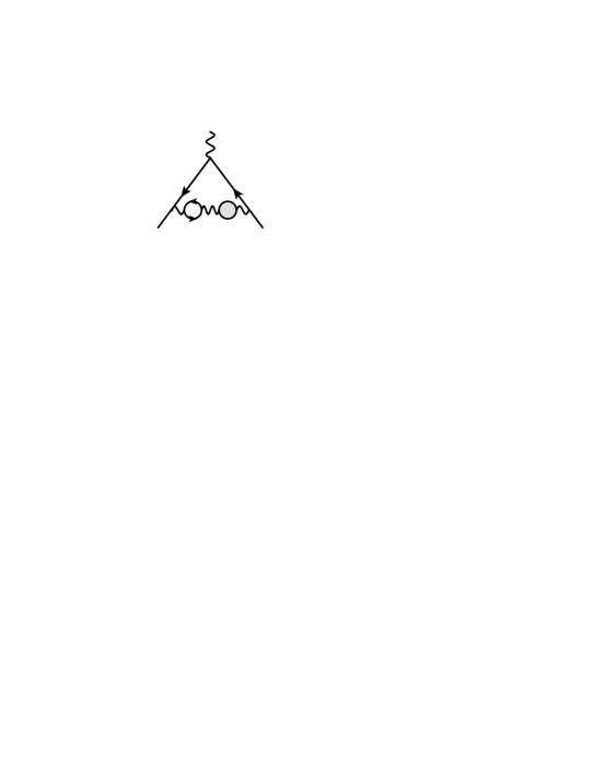
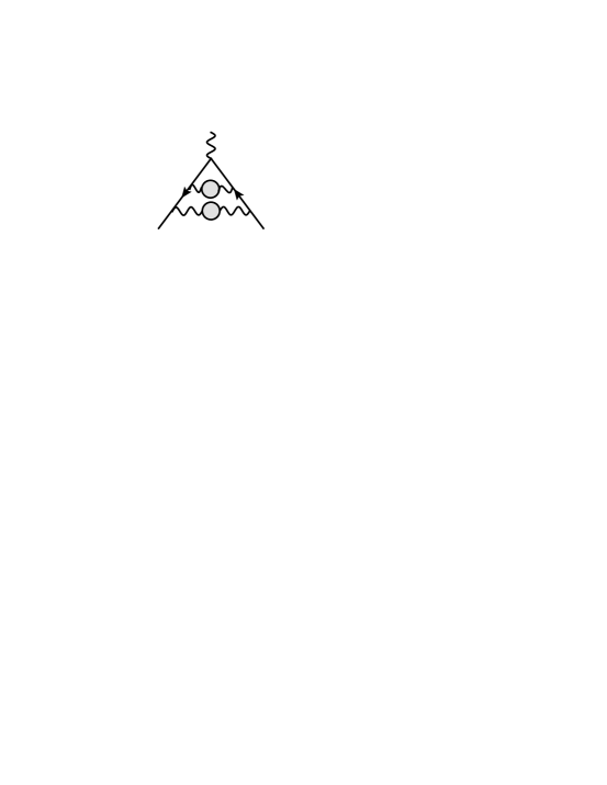
In the first line of Fig. 2 a sample Feynman diagram is shown where the thick solid lines represent the tau leptons. Rows two and three of Fig. 2 show the result of the asymptotic expansion where the graphs left of the symbol have to be expanded in all small quantities, i.e., the external momenta and the muon mass. Thus, the only mass scale of the remaining vacuum integral is the tau lepton mass. The result of the Taylor expansion is inserted into the effective vertex (thick blob) present in the diagram to the right of . Afterwards the remaining loop integrations, which are of on-shell type, are performed.
As a final result we obtain an expansion in with analytic coefficients containing terms. Note that with the help of this method a better accuracy has been obtained than with the numerical approach of Ref. Aoyama:2012wk . Inserting numerical values for the lepton masses leads to
| (4) | |||||
where the ellipsis indicates terms of order which are expected to contribute at order to .
receives contribution from lepton loops starting at two-loop order. Their numerical impact is given by
| (5) |
where the numbers on the right-hand side correspond to the two, three and four loops. It is interesting to note that the three-loop term is only less than a factor four larger than the four-loop counterpart. Furthermore, it is worth comparing the numbers in Eq. (5) to the universal contributions contained in which read Aoyama:2012wk
| (6) | |||||
where the individual terms on the right-hand side represent the results from one to five loops. Note that the four-loop tau lepton term is twice bigger than the five-loop photonic contribution.
4 NNLO hadronic contribution
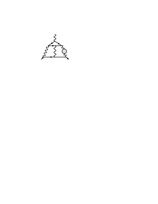
The LO hadronic contribution to the anomalous magnetic moment of the muon is obtained from diagram (a) in Fig. 3. One parametrizes the hadronic contribution (represented by the blob) by the polarization function which appears as a factor in the integrand of the one-loop diagram. In a next step one exploits analyticity of and uses a dispersion integral to introduce its imaginary part,
| (7) |
with . Note that does note include initial state radiative or vacuum polarization corrections. At that point the loop integration and the dispersion integral are interchanged and one obtains
| (8) |
A convenient integral representation for the kernel function , which is the result of the loop integration, is given by
| (9) |
At one-loop order it is possible to obtain analytic results (see Refs. BroRaf68 ; Eidelman:1995ny ). Nevertheless, it is promising to consider in the limit which is justified since the lower integration limit in Eq. (8) is which is bigger than . The expansion of is easily obtained by remembering that it originates from the vertex diagram similar to Fig. 3(a) where the hadronic blob (including the external photon lines) is replaced by a massive photon with mass . The expansion is easily implemented with the help of the program exp Harlander:1997zb ; Seidensticker:1999bb which implements the rules of asymptotic expansions involving a large internal mass (see, e.g., Ref. Smirnov:2013 ). As a result the original two-scale integral is represented as a sum of one-scale integrals which are simple to compute. Using this approach several expansion terms in can be computed. One observes that an excellent approximation for is obtained by including terms up to order .
The approach described in detail for the one-loop diagram can also be applied at two and three loops where exact calculations of the kernel functions are either very difficult or even impossible. In Ref. Kurz:2014wya four expansion terms have been computed which provides an approximation at the per mil level.
A slight complication arises for the contributions involving more than one hadronic insertion, see Figs. 3(d,h,i,j,l). In case they are present in the same photon line formulas similar to Eq. (9) can be derived with two- and three-dimensional integrations. Diagrams of type in Fig. 3 are more involved. Here, we apply a multiple asymptotic expansion in the limits , and ( and are the integration variables) and construct an interpolating function by combining the results from the individual limits.
 |
 |
 |
 |
| (a) LO | (b) | (c) | (d) |
 |
 |
 |
 |
| (e) | (f) | (g) | (h) |
 |
 |
 |
 |
| (i) | (j) | (k) ,lbl | (l) |
The LO result for the hadronic vacuum polarization contribution to can be found in Refs. Davier:2010nc ; Hagiwara:2011af ; Jegerlehner:2011ti ; Benayoun:2012wc ; Jegerlehner:2015stw and NLO analyses have been performed in Refs. Krause:1996rf ; Greynat:2012ww ; Hagiwara:2003da ; Hagiwara:2011af . Our NLO results for the three contributions read
| (10) |
which leads to
| (11) |
in a good agreement with Refs. Hagiwara:2003da ; Hagiwara:2011af . Note that in our analyses no correlated uncertainties are taken into account. Such a rough treatment should not be done at LO but is certainly acceptable at NNLO.
For the individual NNLO contributions we obtain the results
| (12) |
which leads to
| (13) |
It is interesting to note that similar patterns are observed at two and three loops: multiple hadronic insertions are small and the contributions of type (b) involving closed electron two-point functions reduce the contributions of type (a) by about 50%. However, at three-loop order there is a new type of diagram where the external photon couples to a closed electron loop () which provides the largest individual contribution. This is in analogy to the three-loop QED corrections where the light-by-light type diagrams dominate the remaining contributions. In fact, due to the NNLO hadronic vacuum polarization contribution has a non-negligible impact. It has the same order of magnitude as the current uncertainty of the leading order hadronic contribution and should thus be included in future analyses.
An important contribution to is provided by the so-called hadronic light-by-light diagrams where the external photon is connected to the hadronic blob. The NLO part of this contribution is of the same perturbative order as the corrections in Eq. (13). A first-principle calculation of this part is currently not available, however, in Colangelo:2014qya it has been estimated to .
We want to mention that there is a further hadronic contribution where four internal photons couple to the hadronic blob and the external photon couples to the muon line (“internal hadronic light-by-light”). This contribution, which is formally of the same perturbative order as , is currently unknown.
5 Summary and conclusions
For more than a decade the measured and predicted results for the anomalous magnetic moment of the muon show a discrepancy of three to four standard deviations. This circumstance has triggered many publications which try to interpret the deviation with the help of beyond-SM theories. However, before drawing definite conclusions it is necessary to cross check the experimental result by performing an independent high-precision determination of . Furthermore, all ingredients of the theory prediction should be computed by at least two groups independently.
In this contribution we describe the calculation of two classes of four-loop QED contributions to , which up to date only have been computed by one group: the contribution involving tau leptons and the one involving light-by-light-type closed electron loops. Good agreement with the results in the literature is found. To complete the cross check of the four-loop result the non-light-by-light electron contribution, the diagrams involving simultaneously electrons and taus, and the pure-muon contribution have to be computed. From the technical point of view the missing diagram classes have the same complexity as those described in Sections 2 and 3.
As a further topic we have discussed in Section 4 the calculation of the NNLO hadronic vacuum polarization contribution.
Acknowledgments
M.S. would like to thank the organizers of “Flavour changing and conserving processes 2015” for the pleasant atmosphere during the conference. We thank the High Performance Computing Center Stuttgart (HLRS) and the Supercomputing Center of Lomonosov Moscow State University LMSU for providing computing time used for the numerical computations with FIESTA. P.M. was supported in part by the EU Network HIGGSTOOLS PITN-GA-2012-316704. This work was supported by the DFG through the SFB/TR 9 “Computational Particle Physics”. The work of V.S. was supported by the Alexander von Humboldt Foundation (Humboldt Forschungspreis).
References
- (1) G. W. Bennett et al. [Muon g-2 Collaboration], Phys. Rev. D 73 (2006) 072003 [hep-ex/0602035].
- (2) B. L. Roberts, Chin. Phys. C 34 (2010) 741 [arXiv:1001.2898 [hep-ex]].
- (3) R. M. Carey et al., FERMILAB-PROPOSAL-0989.
- (4) D. Hertzog, these proceedings.
- (5) B. Aubert et al. [BaBar Collaboration], Phys. Rev. Lett. 103 (2009) 231801 [arXiv:0908.3589 [hep-ex]].
- (6) F. Ambrosino et al. [KLOE Collaboration], Phys. Lett. B 700 (2011) 102 [arXiv:1006.5313 [hep-ex]].
- (7) S. Eidelman, these proceedings.
- (8) M. Della Morte, B. Jager, A. Juttner and H. Wittig, JHEP 1203 (2012) 055 [arXiv:1112.2894 [hep-lat]].
- (9) F. Burger et al. [ETM Collaboration], JHEP 1402 (2014) 099 [arXiv:1308.4327 [hep-lat]].
- (10) T. Blum, S. Chowdhury, M. Hayakawa and T. Izubuchi, Phys. Rev. Lett. 114 (2015) 1, 012001 [arXiv:1407.2923 [hep-lat]].
- (11) T. Blum, N. Christ, M. Hayakawa, T. Izubuchi, L. Jin and C. Lehner, arXiv:1510.07100 [hep-lat].
- (12) C. Lehner, these proceedings.
- (13) T. Aoyama, M. Hayakawa, T. Kinoshita and M. Nio, Phys. Rev. Lett. 109 (2012) 111808 [arXiv:1205.5370 [hep-ph]].
- (14) S. Laporta, Phys. Lett. B 312 (1993) 495 [hep-ph/9306324].
- (15) P. A. Baikov and D. J. Broadhurst, [hep-ph/9504398].
- (16) J. -P. Aguilar, D. Greynat and E. De Rafael, Phys. Rev. D 77 (2008) 093010 [arXiv:0802.2618 [hep-ph]].
- (17) R. Lee, P. Marquard, A. V. Smirnov, V. A. Smirnov and M. Steinhauser, JHEP 1303 (2013) 162 [arXiv:1301.6481 [hep-ph]].
- (18) P. A. Baikov, K. G. Chetyrkin, J. H. Kuhn, C. Sturm, Nucl. Phys. B 867 (2013) 182 [arXiv:1207.2199 [hep-ph]].
- (19) P. A. Baikov, A. Maier and P. Marquard, Nucl. Phys. B 877 (2013) 647 [arXiv:1307.6105 [hep-ph]].
- (20) A. Kurz, T. Liu, P. Marquard and M. Steinhauser, Nucl. Phys. B 879 (2014) 1 [arXiv:1311.2471 [hep-ph]].
- (21) A. Kurz, T. Liu, P. Marquard, A. V. Smirnov, V. A. Smirnov and M. Steinhauser, arXiv:1508.00901 [hep-ph].
- (22) A. Kurz, T. Liu, P. Marquard and M. Steinhauser, Phys. Lett. B 734 (2014) 144 [arXiv:1403.6400 [hep-ph]].
- (23) M. Beneke and V. A. Smirnov, Nucl. Phys. B 522 (1998) 321 [hep-ph/9711391].
- (24) V. A. Smirnov, Analytic tools for Feynman integrals, Springer Tracts Mod. Phys. 250 (2012) 1.
- (25) A. Pak and A. Smirnov, Eur. Phys. J. C 71 (2011) 1626 [arXiv:1011.4863 [hep-ph]].
- (26) B. Jantzen, A. V. Smirnov and V. A. Smirnov, Eur. Phys. J. C 72 (2012) 2139 [arXiv:1206.0546 [hep-ph]].
- (27) A. V. Smirnov, Comput. Phys. Commun. 185 (2014) 2090 [arXiv:1312.3186 [hep-ph]].
- (28) T. Kinoshita and M. Nio, Phys. Rev. D 70 (2004) 113001 [hep-ph/0402206].
- (29) J. Calmet and A. Peterman, Phys. Lett. B 56 (1975) 383.
- (30) C. Chlouber and M. A. Samuel, Phys. Rev. D 16 (1977) 3596.
- (31) R. Harlander, T. Seidensticker and M. Steinhauser, Phys. Lett. B 426 (1998) 125, arXiv:hep-ph/9712228.
- (32) T. Seidensticker, arXiv:hep-ph/9905298.
- (33) S. J. Brodsky and E. De Rafael, Phys. Rev. 168 (1968) 1620.
- (34) S. Eidelman and F. Jegerlehner, Z. Phys. C 67 (1995) 585 [hep-ph/9502298].
- (35) M. Davier, A. Hoecker, B. Malaescu and Z. Zhang, Eur. Phys. J. C 71 (2011) 1515 [Erratum-ibid. C 72 (2012) 1874] [arXiv:1010.4180 [hep-ph]].
- (36) K. Hagiwara, R. Liao, A. D. Martin, D. Nomura and T. Teubner, J. Phys. G 38 (2011) 085003 [arXiv:1105.3149 [hep-ph]].
- (37) F. Jegerlehner and R. Szafron, Eur. Phys. J. C 71 (2011) 1632 [arXiv:1101.2872 [hep-ph]].
- (38) M. Benayoun, P. David, L. DelBuono and F. Jegerlehner, Eur. Phys. J. C 73 (2013) 2453 [arXiv:1210.7184 [hep-ph]].
- (39) F. Jegerlehner, these proceedings, arXiv:1511.04473 [hep-ph].
- (40) B. Krause, Phys. Lett. B 390 (1997) 392 [hep-ph/9607259].
- (41) D. Greynat and E. de Rafael, JHEP 1207 (2012) 020 [arXiv:1204.3029 [hep-ph]].
- (42) K. Hagiwara, A. D. Martin, D. Nomura and T. Teubner, Phys. Rev. D 69 (2004) 093003 [hep-ph/0312250].
- (43) G. Colangelo, M. Hoferichter, A. Nyffeler, M. Passera and P. Stoffer, Phys. Lett. B 735 (2014) 90 [arXiv:1403.7512 [hep-ph]].
- (44) V. Sadovnichy, A. Tikhonravov, V. Voevodin, and V. Opanasenko, “‘Lomonosov’: Supercomputing at Moscow State University.” In Contemporary High Performance Computing: From Petascale toward Exascale (Chapman & Hall/CRC Computational Science), pp.283-307, Boca Raton, USA, CRC Press, 2013.