MultiDarkLens Simulations: weak lensing light-cones and data base presentation

Abstract

In this paper we present a large database of weak lensing light cones constructed using different snapshots from the Big MultiDark simulation (BigMDPL). The ray-tracing through different multiple plane has been performed with the GLAMER code accounting both for single source redshifts and for sources distributed along the cosmic time. This first paper presents weak lensing forecasts and results according to the geometry of the VIPERS-W1 and VIPERS-W4 field of view. Additional fields will be available on our database and new ones can be run upon request. Our database also contains some tools for lensing analysis. In this paper we present results for convergence power spectra, one point and high order weak lensing statistics useful for forecasts and for cosmological studies. Covariance matrices have also been computed for the different realisations of the W1 and W4 fields. In addition we compute also galaxy-shear and projected density contrasts for different halo masses at two lens redshift according to the CFHTLS source redshift distribution both using stacking and cross-correlation techniques, finding very good agreement.

1 Introduction

Weak gravitational lensing is fast becoming an important tool for measuring the evolution in the expansions of the Universe and the distribution of matter within it. Large scale imaging surveys that are currently being carried out such as DES (The Dark Energy Survey Collaboration, 2005; Flaugher, 2005) and surveys that are planned for the future such as LSST, Euclid and WFIRST (Laureijs et al., 2011; Spergel et al., 2013; Ivezic et al., 2008) will use weak lensing to test theories of dark energy, dark matter and alternatives to General Relativity with unprecedented accuracy. As these new weak lensing measurements become more precise, systematic effects arising from the measurement of gravitational shear from galaxy images and in translating these measurements into constraints on cosmology will become more and more important.

The simplest way to confront theory with weak lensing observations is through a second order statistic such as the shear power spectrum or correlation function as a function of scale and source redshift. In the linear regime of structure formation and under the assumptions that the lensing is weak and the Born approximation is valid these statistics can be predicted straightforwardly, as will be reviewed later (for a review of weak lensing see Bartelmann & Schneider (2001)). As lensing observations become more precise the predictions need to take into account more complicated effects. In practice the redshift of individual galaxies need to be measured photometrically which introduces errors and outliers and the surveyed area is a complicated shape with many masked regions which introduces correlations between the measurements of the shear power spectrum or correlation function at different scales which need to be measured precisely. In addition, the gravitational evolution of structure on the relevant scales is not entirely linear, but includes nonlinear structures and even baryonic effects. Then the lensing itself on a galaxy-by-galaxy bases is not always weak in the sense that higher order lensing effects can be safely ignored. These effects can only be addressed with simulations although in some cases analytic methods can be used that are calibrated or fit to simulations. The difficulties in measuring the shear from individual galaxy images is another important, but separate problem that is not directly related to what is discussed here.

In this paper we present the first set of a series of weak lensing simulations that will be provided to the community through a web portal. The intention is to create high quality simulations that can be used by any group to improve techniques and analyse survey data. The underlying cosmological simulation is the BigMDPL simulation (Prada et al., 2014). The light-cone construction and ray-tracing through this simulation is done with the GLAMER code (Metcalf & Petkova, 2014; Petkova et al., 2014). Shear maps, shear catalogs and some analysis tools are provided. The BigMDPL is big enough to provide many independent light-cones and its resolution is high enough to resolve the relevant nonlinear structures. GLAMER calculates the light paths, shear and convergence without resorting to the weak lensing approximation or the Born (unperturbed light paths) approximation so that the impact of such approximations can be evaluated. The first fields reported on here are in the shape of the W1 and W4 fields observed in the VIPERS survey (Guzzo et al., 2014).

The paper is organised as follows: in section 2 we describe the cosmological simulations used; in section 3 we present the methodology adopted in constructing the lens density maps as well as our multi-plane ray-tracing code. In section 4 we present our weak lensing results. Section 5 is a summary of conclusions and discussion.

2 The Big MultiDark Simulation

In this work we perform full ray-tracing simulations with the matter density distributions extracted from the BigMDPL simulation (Prada et al., 2014). This simulation has been performed to meet the science requirements of the BOSS galaxy survey, i.e. the numerical requirements for mass and force resolution that allow one to well resolve those haloes and subhaloes that can host typical BOSS massive galaxies at $z\sim 0.5$. This allows for the creation of mock catalogs with appropriate galaxy bias and clustering. The simulation is in a $\mathrm{\Lambda}$CDM universe comprised of $3840^{3}$ particles in a box of 2.5 comoving Gpc/$h$ on a side. Initial conditions have been generated at redshift $z_{init}=100$ using GINNUNGAGAP publicly available full MPI-OpenMP initial conditions generator code that uses Zeldovich approximation with an number of particles only limited by the computer resources. The simulation has been run with the L-GADGET-2 code (see Klypin et al. (2014), for details). The cosmological parameters have been chosen to be consistent with the latest fits to the Planck data (Planck Collaboration et al., 2013). The mass and force resolutions are $2.36\times 10^{10}h^{-1}M_{\odot}$ and $10h^{-1}$kpc at low redshift – for the high redshift snapshots ($z>2$) a value of $30h^{-1}$kpc is used. The numerical parameters were set to meet the requirements after the completion of many tests that studied the convergence for the correlation function and circular velocities for haloes and their subhaloes (Klypin et al., 2013). The choice of parameters enables the simulation to resolve well the internal structure of all collapsed systems identified with a parallel version of the bound density maximum (BDM) algorithm (Klypin & Holtzman, 1997; Riebe et al., 2013), thus, making it possible to connect them with BOSS-like galaxies (Prada et al., 2014; Rodriguez et al., 2015). From the cosmic shear point of view this allows us to measure the shear-shear correlation function down to small scales and construct cosmic shear power spectrum that is very accurate up to $l=10^{4}$ as will be shown. This maximum limit, in the angular mode $l$, is much larger than the value expected to be reachable by the future wide field surveys.

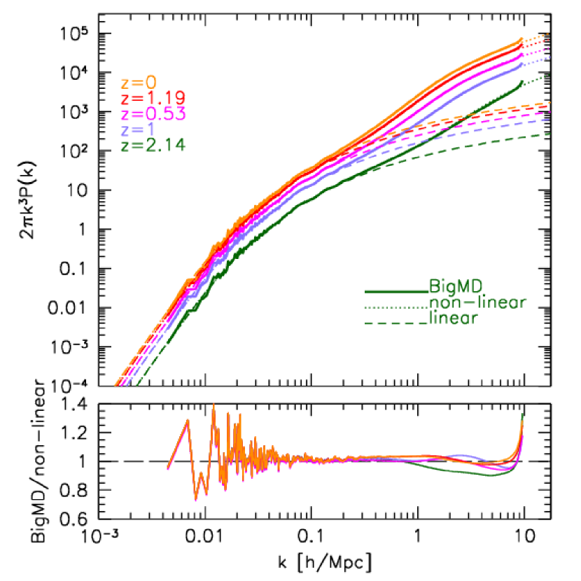
Figure 1: Matter power spectra measured at five different redshifts in the simulation (solid line). The dashed curves show the linear prediction at the corresponding redshifts computed using the CAMB code. The dotted curves show the non-linear predictions inputting the corresponding linear power spectrum in the extended version of Halofit (Smith et al., 2003) by Takahashi et al. (2012). The bottom panel shows the ratio between the non-linear power spectrum measured in the simulation and the one predicted by the analytical recipe.

In Fig. 1 we show the matter power spectra at five different redshifts computed from the particle distribution taken from some simulation snapshots (solid curves) as indicated in the figure label. Given the large amount of particles and the box-size, the power spectra have been computed on a mesh of $7680^{3}$ up to a Nyquist frequency of $k=9.65$ $h/$Mpc which correspond to 650 kpc$/h$ in comoving scale. In the same figure linear (dotted) and non-linear (dashed) predictions obtained from CAMB (Lewis et al., 2000) are displayed. For the non-liner matter power spectrum model we adopt an extended version of the Halofit Model (Smith et al., 2003) from Takahashi et al. (2012) build on the corresponding linear power spectrum. The figure shows the very good agreement between the non-linear recipe for the power spectrum and the one measured in the simulation with an uncertainty well below two percents for modes between 0.1 and 1 $h$/Mpc. For larger modes, below the Nyquist value of the mesh, the deviations from snapshots with redshifts $z>0$ reach at most four percent with larger deviations at higher redshift.

3 Methodology

In this section we describe how the lensing light-cones have been constructed from the N-body simulation and the ray-tracing procedure. The method used in this paper is similar to those presented in Vale & White (2003) and Hilbert et al. (2009). The particles are projected onto different lens planes that are distributed along the line of sight and filling the light-cone up to redshift $z=2.3$. Petkova et al. (2014) have studied the impact of the number of lens planes on lensing quantities such as the deflection angle and the convergence. They found that the error in the convergence, even in cases of strong lensing, is less than 5% if planes are separated by about 300 Mpc/$h$. In our case, we choose a distance between each lens plane of 161 Mpc/$h$ which is $N=24$ lens planes out to 3.9 Gpc/$h$ comoving. In accordance with this number, we select 24 snapshots out of the 80 available in the simulation, for which the redshift is the closest to the estimated redshifts of the planes.

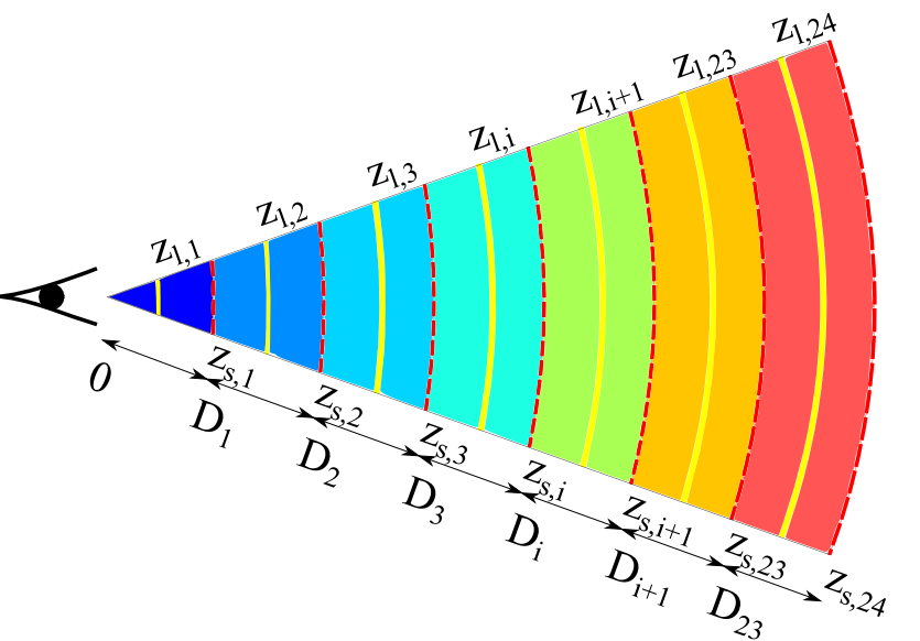
Figure 2: Schematic representation of the light-cone construction from the simulation. The slices in colour show the portion of the matter extracted from each snapshots with comoving distance between $D_{i}$ and $D_{i+1}$, within the aperture of the field of view. Given $D_{i}$ and $D_{i+1}$ we define the lens redshift at their half distance $z_{l,i}=z[(D_{i}+D_{i+1})/2]$ and the source redshift $z_{s,i}=z[D_{i+1}]$.

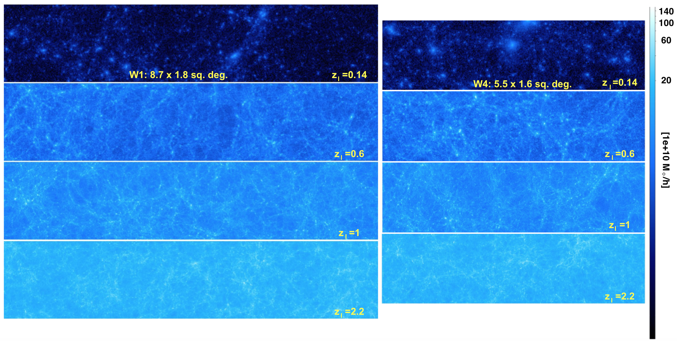
Figure 3: The two dimensional surface matter density distribution in four lens planes as extracted from the simulation: $z_{l}=$ 0.14, 0.6, 1 and 2.2, from top to bottom respectively. While the left panels have the geometry of the W1 field, the right ones of W4; with resolution $5220\times 1080$ and $3300\times 960$ pixels, respectively. We remind the reader that the effective sizes of the two fields in the figure may not be properly in scale with each other.

3.1 Light-cone geometry

For the analyses conducted in this work, we build two different light-cones geometries – many other will be available in our database – one covering a region of $8.7\times 1.8$ deg² and another a region of $5.5\times 1.6$ deg², that mimic the W1 and W4 fields observed by the VIPERS extragalactic survey (Guzzo et al., 2014), respectively. In order to maximise the number of independent light-cone realisations, we remap the 2.5³ (Gpc/$h$)³ cubical volume of the simulation using BoxRemap (Carlson & White, 2010). BoxRemap takes advantage of the periodicity of the simulated box to break it into cells, which are then translated by integer offsets to form cuboids. The remapping procedure keeps local structures intact. We adjust the parameters in order to maximise the number of light-cones that can be embedded in the comoving simulation volume. In this adjustment, we avoided configurations in which the original cube is remapped into a very long and narrow cuboid, where we found that particles can be lost or are not well remapped. For the W1 lightcones, the original box is remapped into a $3875\times 588\times 122$ Mpc/$h$ cuboid. For W4, the shape is $3875\times 373\times 108$ Mpc/$h$. From these cuboids, the numbers of independent realisations that we were able to create are respectively 54 and 99 for the W1 and W4 fields. Their properties are summarised in Table 1.

Table 1: Summary of simulated light-cones

Field name	Size [deg2]	# Realisations
W1	$8.7\times 1.8$	54
W4	$5.5\times 1.6$	99

In Fig. 2 we show a schematic representation of a light-cone construction. For each snapshot $i$, we remap its particles to form the cuboid shape given above. For each light-cone and each snapshot, we recenter the particle positions according to its centre in the cuboid and convert its particle positions from Cartesian to spherical coordinates. Particles with radial comoving distance between $D_{i}$ and $D_{i+1}$ and inside the light-cone aperture are projected onto a 2D angular mesh using the ’cloud-in-cell’ technique Hockney & Eastwood (1988). This procedure is repeated for the M light-cones in the cuboid, thus producing M independent lens planes at redshift $z_{l,i}=z[(D_{i}+D_{i+1})/2]$ with $i\in[1,N]$.

In Fig. 3 we show the projected mass per pixel in unit of $10^{10}M_{\odot}/h$, distributed on four different lens planes as indicated in the labels of the figure. Right and left panels refer to W1 and W4 geometry resolved with $5220\times 1080$ and $3300\times 960$ pixels, respectively. The effective sizes of the two fields in the figure may not be properly in scale with each other. No truncation in the large scale structures is observed.

3.2 Ray-Tracing through multiple planes

We run our ray-tracing code GLAMER on each of the M realisations of N lens planes. The ray-tracing code is run for N source redshifts in the light-cone, i.e. those corresponding to the boundaries between 2 consecutive snapshots $z_{si}=D_{i+1}$. In Fig. 4 we show the number of planes through which we perform multi-plane ray-tracing as a function of the source redshift. The vertical dashed lines show $z_{s}=0.5$, 1 and 2.3, that we will be considered as reference in presenting some lensing measurements in the following sections. The particle distributions from the simulation snapshots are projected onto different matter density planes; these are given as input to GLAMER (Metcalf & Petkova, 2014; Petkova et al., 2014) to trace the light-rays from different source redshifts to the observer – although technically the rays are shot the other way around to be sure that all rays intersect the the observer.

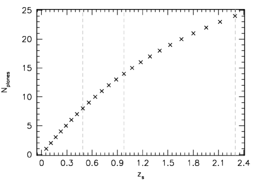
Figure 4: Number of lens planes through which the ray-tracing is performed as a function of the source redshift. The vertical dashed lines show as a reference $z_{s}=0.5$, 1 and 2.3 that we will be considered as reference in presenting some lensing measurements in the following sections.

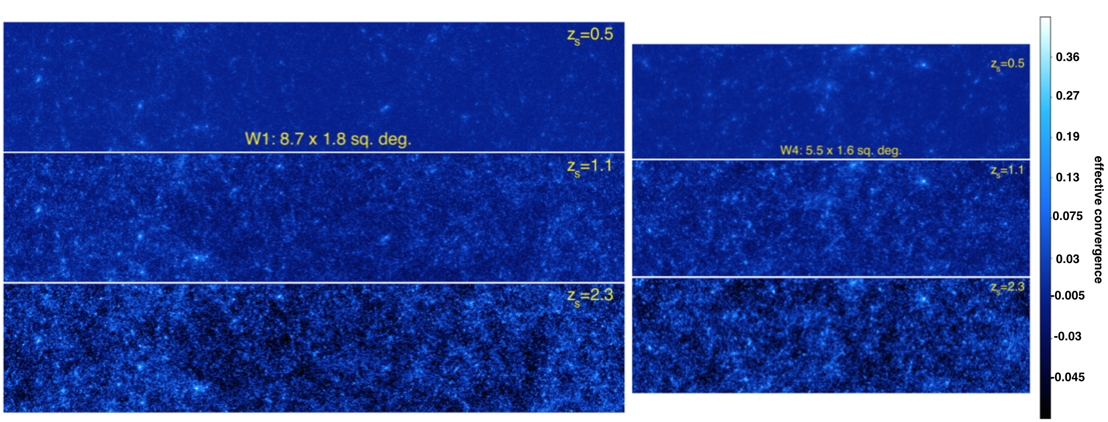
Figure 5: Effective convergence maps of one realisation of the W1 (left) and W4 (right) light-cones for sources located at three different fixed redshifts. From top to bottom we show the effective convergence constructed from our ray-tracing pipeline considering all the mass in the light-cone up to $z_{s}=0.5$, $1.1$ and $2.3$. The convergence maps have the same resolution of the initial mass density maps namely corresponding to an angular resolution of 6 arcsec per pixel.

A few definitions are required. If the angular position on the sky is ${\boldsymbol{\theta}}$ and the position on the source plane expressed as an angle (the unlensed position) is ${\boldsymbol{\beta}}$, then a distortion matrix ${\bf A}$ can be defined as

$${\bf A}\equiv\frac{\partial{\boldsymbol{\beta}}}{\partial{\boldsymbol{\theta}}}=\left(\begin{array}[]{cc}1-\kappa-\gamma_{1}&\gamma_{2}-\varsigma\\ \gamma_{2}+\varsigma&1-\kappa+\gamma_{1}\end{array}\right)\ .$$ (3)

The traditional decomposition of this matrix is shown, where $\kappa$ is called the convergence and ${\boldsymbol{\gamma}}$ represents the shear. The component $\varsigma$ is very small torsion which is related to the rotation of the image. The torsion is of order $\sim|\gamma|^{2}$ (Petkova et al., 2014) and for weak lensing very small, but will be retained here for completeness.

When there is a single lens plane, the convergence can be expressed as a dimensionless surface density,

$$\kappa({\boldsymbol{\theta}})=\frac{\Sigma({\boldsymbol{\theta}})}{\Sigma_{\rm crit}}\ ,$$ (4)

where

$$\Sigma_{\rm crit}\equiv\dfrac{c^{2}}{4\pi G}\dfrac{D_{l}}{D_{s}D_{ls}}$$ (5)

is called the critical density, $c$ is the speed of light, $G$ is Newton’s constant and $D_{l}$ $D_{s}$ and $D_{ls}$ are the angular diameter distances between observer-lens, observer-source and source-lens, respectively. In general, with multiple lens planes, this is not the case however.

The deflection caused by a lens plane, ${\boldsymbol{\alpha}}$, is related to the surface density on the plane, $\Sigma({\bf x})$, through the differential equations

$$\nabla^{2}\phi({\bf x})=\frac{4\pi G}{c^{2}}\Sigma({\bf x})\leavevmode\nobreak\ \leavevmode\nobreak\ \leavevmode\nobreak\ ,\leavevmode\nobreak\ \leavevmode\nobreak\ \leavevmode\nobreak\ {\boldsymbol{\alpha}}({\bf x})=\nabla\phi({\bf x}).$$ (6)

where the derivatives are with respect to the position on the lens plane. These equations are solved on each source plane by performing a Discrete Fourier Transform (DFT) on the density map, multiplying by the appropriate factors and then transforming back to get a deflection map with the same resolution as the density map. With the same DFT method the shear caused by each plane is simultaneously calculated. In order to reduce boundary effects, due to non-periodic conditions, before going in the Fourier space the maps are enclosed in a zero-paddling region. Because the rays are propagated between planes assuming a uniformly distribution of matter, the matter that has been projected onto the planes over-counts the mass in the universe. To correct for this the ensemble average density on each plane is subtracted. This way each plane has zero total mass on average and the average redshift-distance relation is preserved.

After the deflection and shear maps on each plane are calculated the light-rays are traced from the observers through the lens planes out to the desired source redshift. The shear and convergence are also propagated through the planes as detailed in Petkova et al. (2014). GLAMER preforms a complete ray-tracing calculation that takes into account non-linear coupling terms between the planes as well as correlations between the deflection and the shear. No weak lensing assumption is made at this stage. The rays are shot in a grid pattern with the same resolution as the mass maps.

In the Figures 5 we display the convergence maps for one realisation of the W1 (left) and W4 (right) fields at three different source redshifts, increasing from top to bottom as indicated in the caption. We emphasise that in doing the multi-plane ray-tracing we have followed the ray bundles through $N=24$ lens plane up to redshift $2.3$, $15$ up to redshift $1$ and $8$ up to $z=0.5$.

3.3 CFHTLS source redshift distribution

Another important ingredient that needs to be taken into account when producing lensing simulations is the redshift distribution of the sources. Here we consider the CFHTLens source redshift distribution (Hildebrandt et al., 2012) as computed within the W1 and W4 fields. In Fig. 6 we show with the dashed curve the redshift distribution of the sources observed in the two fields by CHFTLens, for comparison the solid histogram displays the distribution extracted from one realisation of the W1 field. Since the impact of the source galaxy clustering on lensing statistics is beyond the purpose of this first work, the location of the sources within the field of view is performed randomly. The tool for extracting the lensing catalogue with a desired source redshift distribution and a generated light-cone is also available in our database. Upon request, users can also ask for an effective convergence map according to a desired source redshift distribution table.

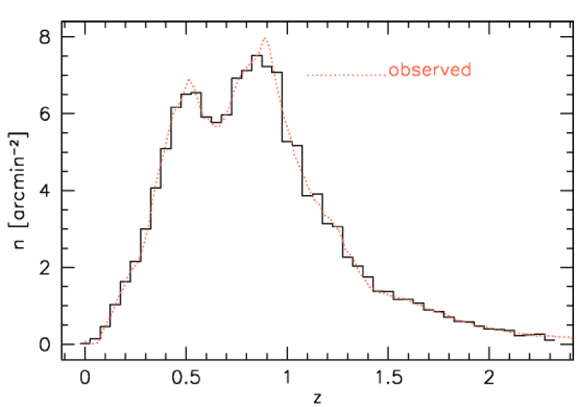
Figure 6: Source redshift distribution adopted to compute the shear catalogue from our light-cone realisations. The dashed curve represents the CFHTLS source redshift distribution, while the solid histogram refers the one obtained from one realisation of the W1 field, randomly distributing the sources in the field-of-view.

Once the redshift and the source positions within the field of view are known, we compute the corresponding lensing properties – convergence and shear – linearly interpolating the quantities in the field and between different planes. In this way we extract self-consistent catalogs for the desired field of view according to a specific source redshift distribution. For each field of view, we randomly draw eight catalogues, hence in total 432 and 891 lensing catalogues for W1 and W4, respectively.

In our online achieve we provide a tool that allows a user to calculate shear and convergence maps and catalogs with any desired source redshift distribution.

4 Cosmic-Shear and Lensing Signals

The convergence power spectrum, to first order, can be expressed as an integral of the 3D matter power spectrum computed from the present time up to the source redshift (Bartelmann & Schneider, 2001). In this section we review the calculation of the cosmic shear power spectrum adopting the Born approximation (light rays travel along unperturbed paths) and the weak lensing proximation (ignore all terms higher than first order in $\kappa$ and $\gamma$). Since our ray-tracing simulations do not make these approximations we can check their validity by comparing the two methods of calculating the shear power spectrum.

Following an unperturbed light-ray through inhomogeneous universe it is possible to calculate the first order convergence, $\kappa$, in terms of the matter over density, $\delta=(\rho-\overline{\rho})/\overline{\rho}$, that it passes through

$$\kappa(w_{s},\boldsymbol{\theta})=\dfrac{3H_{0}\Omega_{m}}{2c^{2}}\int_{0}^{w_{s}}\mathrm{d}w\dfrac{f(w)f(w_{s}-w)}{f(w_{s})}\dfrac{\delta(f(w)\boldsymbol{\theta},w)}{a(w)}$$ (7)

where $f(w)$ represents the radial function:

$$f(w)=\begin{cases}K^{-1/2}\sin\left(K^{1/2}w\right)&\;\;\;(K>0)\\ w&\;\;\;(K=0)\\ (-K)^{-1/2}\sinh\left[\left(-K\right)^{1/2}w\right]&\;\;\;(K<0)\\ \end{cases}$$ (8)

depending on whether the curvature of the universe K is positive, zero or negative; and $a=1/(1+z)$ the scale factor. The convergence power spectrum for sources at a fixed redshift is:

$$\langle\hat{\kappa}(\boldsymbol{l})\hat{\kappa}*(\boldsymbol{l}^{\prime})\rangle=\left(2\pi\right)^{2}\delta_{D}(\boldsymbol{l}-\boldsymbol{l}^{\prime})P_{\kappa}(l)$$ (9)

with

$$P_{\kappa}(l)=\dfrac{9H_{0}^{4}\Omega_{m}^{2}}{4c^{4}}\int_{0}^{w_{s}}\mathrm{d}w\dfrac{f^{2}(w_{s}-w)}{f^{2}(w_{s})a^{2}(w)}P_{\delta}\left(\dfrac{l}{f(w)},w\right)\,.$$ (10)

(Kaiser, 1998, 1992) Considering a normalised source redshift distribution $p(z_{s})\mathrm{d}z_{s}=g(w_{s})\mathrm{d}w_{s}$ we can write down the associated convergence power spectrum of a population of galaxies as

$$P_{\kappa}(l)=\dfrac{9H_{0}^{4}\Omega_{m}^{2}}{4c^{4}}\int_{0}^{w_{s}}\mathrm{d}w\dfrac{W^{2}(w)}{a^{2}(w)}P_{\delta}\left(\dfrac{l}{f(w)},w\right)\,,$$ (11)

where $W(w)$ represents the weighted source redshift distribution:

$$W(w)=\int_{w}^{\infty}\mathrm{d}w^{\prime}g(w^{\prime})\dfrac{f(w^{\prime}-w)}{f(w^{\prime})}\,.$$ (12)

In the same way we can obtain an estimate of the effective convergence map given a source redshift distribution by weighting the contributions of the different constructed planes.

In real space, the direct measurement of weak lensing is the two point shear correlation functions $\xi_{+}$ and $\xi_{-}$ that can be obtained from galaxy ellipticity measurements $\epsilon_{t}$ and $\epsilon_{\times}$ (aligned and at 45 degrees to the line connecting to galaxies)– tangential and cross component, respectively – by averaging over galaxy pairs with angular distance $|\boldsymbol{\theta}_{i}-\boldsymbol{\theta}_{j}|$ in a bin $\theta$:

$$\xi_{\pm}(\theta)=\dfrac{\sum_{ij}\omega_{i}\omega_{j}\left[\epsilon_{t}(\boldsymbol{\theta}_{i})\epsilon_{t}(\boldsymbol{\theta}_{j})\pm\epsilon_{\times}(\boldsymbol{\theta}_{i})\epsilon_{\times}(\boldsymbol{\theta}_{j})\right]}{\sum_{ij}\omega_{i}\omega_{j}}\,$$ (13)

(Schneider et al., 2002) where $\omega$ represents the weight obtained from galaxy shape measurement pipeline. The two point shear correlation functions can be related to the cosmic shear power spectrum by the following relation:

$$\xi_{+/-}=\dfrac{1}{2\pi}\int_{0}^{\infty}\mathrm{d}l\leavevmode\nobreak\ lP_{\kappa}(l)J_{0/4}(l\theta)\,,$$ (14)

where $J_{0}$ and $J_{4}$ are the Bessel functions and we have set the B-mode power spectrum equal to zero in agreement with the weak lensing prediction.

It is also common to measure the variance of the convergence field filtered with window function or aperture

$$M\left(\theta\right)=\int_{0}^{\theta}d^{2}\theta^{\prime}\leavevmode\nobreak\ W(|\theta^{\prime}|)\kappa(\boldsymbol{\theta}^{\prime})$$ (15)

with the normalisation

$$\int_{0}^{\theta}d\theta\leavevmode\nobreak\ W(\theta)=0.$$ (16)

The convergence $\kappa$ is not directly measured in a shear survey, but Schneider (1996) showed that $M\left(\theta\right)$ is equivalent to

$$M\left(\theta\right)=\int_{0}^{\theta}d^{2}\theta^{\prime}\leavevmode\nobreak\ Q(|\theta^{\prime}|)\gamma_{t}(\boldsymbol{\theta}^{\prime})$$ (17)

with

$$Q\left(\theta\right)=\frac{2}{\theta^{2}}\int_{0}^{\theta}d\theta^{\prime}\leavevmode\nobreak\ \theta^{\prime}W(\theta^{\prime})-W(\theta)$$ (18)

which can be measured from the tangential ellipticities of galaxies. We will investigate a few choices for $W(\theta)$ in section 4.

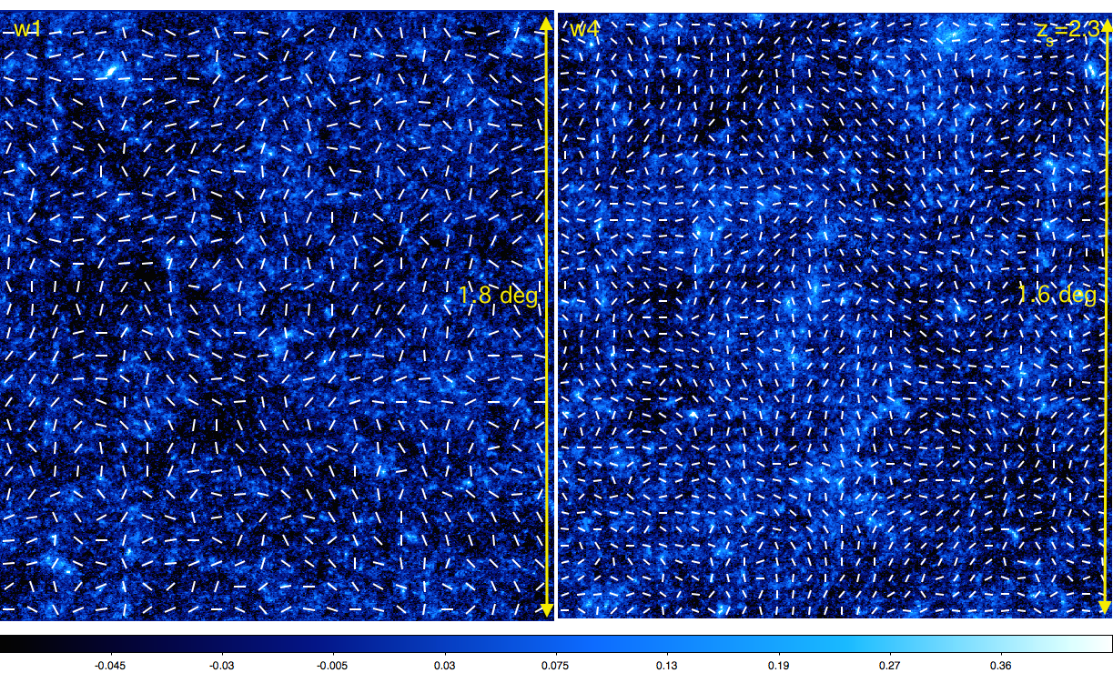
Figure 7: Effective convergence maps for sources at redshift $z_{s}=2.3$ for a square region the W1 (left) and the W4 (right) fields. In this case we show sticks – that in each panel have the same angular size – representing the direction of the corresponding shear field.

In Fig. 7 we show the effective convergence maps of two cropped regions in the W1 and W4 fields of view with 1.8 deg and 1.6 deg on a side, respectively, pixels have a resolution of $6$ arcsec. The convergence maps have been constructed considering all the matter density distribution in the light-cone up to redshift $z_{s}=2.3$. In each squared panel the sticks represent the directions of the corresponding shear field, which are consistently tangentially directed around large density peaks.

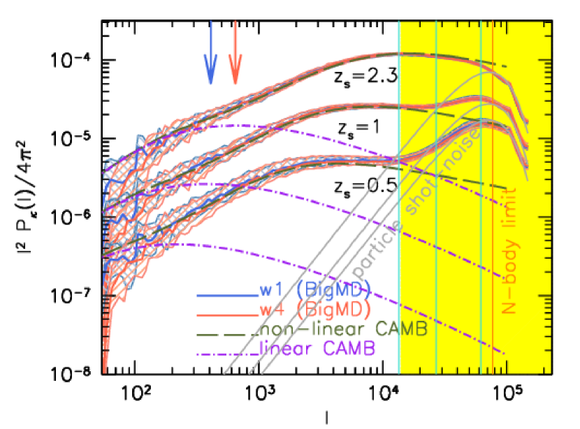
Figure 8: Cosmic-shear power spectrum from the simulation (thick solid curve) considering sources located at different redshifts, as indicated in the label. The cosmic shear power spectrum predictions from the linear and the non-linear Halo-Fit matter power spectrum are also shown in the figure with dashed and dot-dashed curve, respectively. The two coloured vertical arrows indicate, for the corresponding colour type, the multipole scale which sample the largest coordinate within the field of view. The three cyan vertical lines (from left to right) indicate the angular scales mode above which the power spectrum is dominated by particle shot-noise at source redshift $z_{s}=0.5$, $1$ and $2.3$, respectively. The yellow shaded area indicates the region, starting from the mode corresponding to $96$ arcsec, below which any of the considered source redshift maps are not affected by particle shot-noise. The grey curves show the particle shot-noise contribution at the three considered source redshifts.

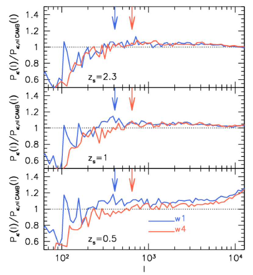
Figure 9: Ratio between the measured cosmic shear power spectra in the simulated fields of view and the non-linear predictions by (Takahashi et al., 2012) at three different redshifts. The two coloured vertical arrows indicate, for the corresponding color type, the multipole scale which sample the largest coordinate within the field of view in the W1 and W4 fields.

In Fig. 8 we show the convergence power spectrum computed for three different fixed source redshifts from the 54 and 99 realisations of the W1 and W4 fields, respectively. The solid blue and red curves represent the median on the different light-cone realisations, while the corresponding shaded region encloses the first and the third quartile of the distribution at fixed $l$. The two coloured vertical arrows indicate, for the corresponding color type, the multipole scale which sample the largest coordinate of the field of view. The three cyan vertical lines indicate the minimum scale (from left to right) up to which the power spectra of the maps at redshift $z_{s}=0.5$, $1$ and $2.3$ are not affected by particle shot-noise. The orange vertical line – labelled as N-body limit – corresponds to $l_{N}=1/\sigma_{N}$ with $\sigma_{N}=0.05N_{part}^{-1/3}$ and $N_{part}=3840^{3}$, as discussed also by Vale & White (2003). The yellow shaded area indicates the region below which any the considered source redshift maps are not affected by particle shot-noise – starting from the mode corresponding to $96$ arcsec. We remind the reader that the minimum scale where particle noise start to become worthy of consideration depends on the source redshift and is of the order of $24$ arcsec for $z_{s}=2.3$. The grey curves show the particle noise contribution (Vale & White, 2003) at the three corresponding source redshifts that can be read as:

$$l^{2}P_{\kappa,\,\textrm{SN}}(l)\propto\dfrac{l^{2}}{N_{part}^{3}}\exp\left(-l^{2}/l^{2}_{SN}\right)\,$$ (19)

with $l_{SN}=2\pi/(3\theta_{pix})$ ($\theta_{pix}=6\,\textrm{arcsec}$).

The dashed green and the dot-dashed magenta curves show the convergence power spectra computed by integrating the linear and non-linear power spectra from CAMB up to the corresponding considered source redshift. From the figure we notice that the agreement between the power spectrum computed from the ray-traced field of view and from non-linear CAMB agree quite well with a difference of the order of only few percents. This is more evident in Fig. 9 where we present the ratio between the convergence power spectrum measured in the two fields W1 and W4 and the one computed using equation (10) adopting the non-linear CAMB matter power spectrum. The figure shows that the agreements between the theoretical modelling of the cosmic shear and the shear measured from ray-tracing simulations agree within $5\%$ up a scale of $l\approx 3000$ which represents the largest multipole up to which future extragalactic surveys are expected to measure the lensing power spectrum. Small differences between simulations and non-linear predictions may be due to non-linear lensing effects, cosmic variance, or to the fact that the non-linear modeling of the power spectrum by (Takahashi et al., 2012) does not quite capture the small scale clustering of the matter in the numerical simulation. In the figure it can be seen that the limited size of the field of view is responsible for the drop in the signal at small multiples (large scales) which gives an idea of the accuracy with which the power spectrum normalisation can be measured given the size of the field of view.

Differences between analytic models and simulations may be also due to the fact that the analytic calculations are made under the assumption of the Born approximation, where the ray paths approximated as what they would be in a homogeneous metric, and discarding lens-lens coupling. To quantify this we re-run GLAMER again on all the fields and realizations turning off the Born approximation. In Figure 10 we show the relative residuals between the median convergence power spectra computed for the two fields with and without the Born approximation, for three different source redshifts. As noticed by Schäfer et al. (2012) performing an analytic perturbative expansion in the light path the Born approximation is an excellent approximation for weak cosmic lensing but fails at small scales where strong and quasi-strong lensing takes place. From the figure we notice also that the relative difference at small scales depends on the number of lens planes considered in the ray-tracing and so on the source redshift.

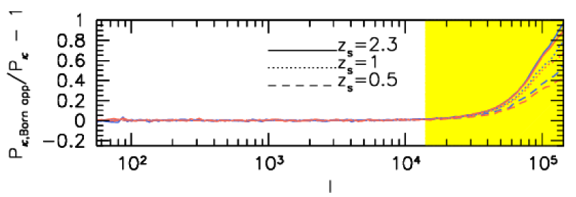
Figure 10: Relative residuals between the median convergence power spectra computed from the different realisations of the two fields assuming or discarding the Born approximation, for the three considered source redshifts. As in the previous figures blue and red colors refer to the W1 and the W4 field, respectively. The yellow shaded area is like in Figure 8.

4.0.1 Power Spectrum Correlation Matrix

To accurately measure the cosmological parameters from the lensing power spectra of the W1 and W4 light-cones, the cross-correlation between measurements of the power at different scales must be known. This can be quantified by the power spectrum correlation matrix that is mainly influenced by the specific survey geometry and the non-Gaussian nature of the density distribution.

From the different light-cones realisations we build up the covariance matrix from the definition:

$$M(l,l^{\prime})=\langle P_{\kappa}(l)-\bar{P}_{\kappa}(l)\rangle\langle P_{\kappa}(l^{\prime})-\bar{P}_{\kappa}(l^{\prime})\rangle$$ (20)

where $\langle\bar{P}_{\kappa}(l)\rangle$ represents the best estimate of the power spectrum at the mode $l$ obtained from the median of all the corresponding light-cone realisations and $P_{\kappa}(l)$ represents the measurement of one realisation. The matrix is then normalised as follows:

$$m(l,l^{\prime})=\dfrac{M(l,l^{\prime})}{\sqrt{M(l,l)M(l^{\prime},l^{\prime})}}\,.$$ (21)

The covariance matrix constructed in this way accounts both for a Gaussian and non-Gaussian contribution arising from mode coupling due to non-linear clustering and for the survey geometry (Scoccimarro et al., 1999; Cooray & Hu, 2001; Harnois-Déraps et al., 2012; Sato & Nishimichi, 2013). Off-diagonal terms with value near unity indicate high correlation while values approaching zero indicate no correlation.

In Fig. 11 we show the normalised covariance matrices for the W1 (top) and the W4 (bottom) fields of view assuming $\Delta l\approx 0.075$. We again show the cases where sources are fixed and located at three different redshifts, increasing from left to right, as indicated in the label. It is interesting that at small redshifts the correlation of the power spectrum between two different $l$-modes is stronger than at higher redshifts. For sources with $z_{s}=2.3$ correlations are present only at small scales, large $l$ modes. The enhancement of the correlation at large $l$ (small scales) at low redshift is intrinsic to the non-Gaussian statistics of the halo clustering. From the figure we also notice that the low redshift covariance matrices depend on the considered field of view. Because W1 is a longer stripe the enhancement in the correlation occur already at larger scales with respect to W4.

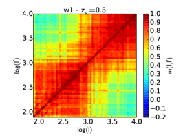
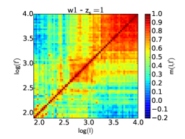
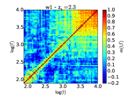
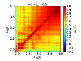
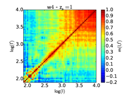
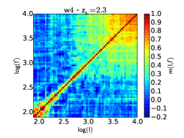
Figure 11: Normalised cosmic shear covariance matrices for the two fields of view – W1 in the top panels and W4 in the bottom, respectively. As indicated in the label the matrices are presented considering sources at three different fixed source redshifts.

4.0.2 one-point probability distributions

The one-point probability distribution of the field can also help in distinguishing the underling cosmological model (Takahashi et al., 2011; Pace et al., 2015; Giocoli et al., 2015). In the top-panels of Fig. 13 shows the probability distribution function of the convergence (left), absolute shear (centre) and magnification (right) averaged over the all 153 realisations of the two fields from the original maps having an pixel resolution of $6$ arcsec.

From the figure the different line style curves, with different corresponding colours, represent the median over all the realisations and the shaded region encloses the first and the third quartile at fixed values. As was done for the power spectrum, we show the distributions for three different fixed source redshifts $z=0.5$, 1 and 2.3. In the convergence PDF we notice that while the average value of the field remains null, the shape of the distribution enlarges as the source redshift increases giving also rise to an high value tail. The same behaviour is reflected in the shear and the magnification even if the average value of the first increases with $z_{s}$. We remind the reader that the distributions depends on the pixel sizes of the maps that have been constructed which in this case is 6 arcsec. To better interpret those results, in Fig 13 we show the median fraction of pixels as a function of the source redshift with convergence, shear and magnification (left, central and right panel, respectively) above a given minimum threshold. The shaded regions enclose the first and the third quartile of the distributions at fixed $z_{s}$. In the bottom panels of Fig. 13 we show the one-point distribution of the maps degraded to a resolution of $96$ arcsec per pixels that, as discussed already for the cosmic shear power spectrum, corresponds to scale at which the different source redshift maps in the light-cone are not affected by particle shot-noise. The small sub-panels show the one-point distributions of the maps with $\theta_{pix}=6$ arcsec in the same axis scales, for a more direct comparison. From the figures we notice that the distribution function of the maps with $\theta_{pix}=96$ arcsec are less spread than those computed from the maps with $\theta_{pix}=6$ arcsec for a combination of two effects ($i$) the quenching of the particle noise mainly present in the maps with $z_{s}=0.5$ and for low values of the distributions and ($ii$) the disappearance of high density peaks due to loss of the resolution and of resolving cluster cores.

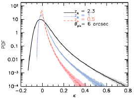
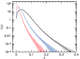
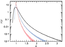
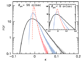
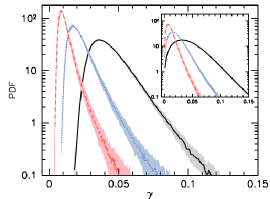
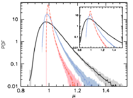
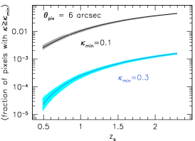
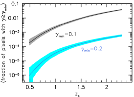
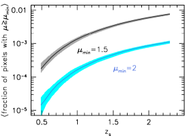
Figure 12: Top panels: median convergence (left), shear (centre) and magnification (right) probability distribution function measured in the different W1 and W4 light-cone realisations for sources at three different redshifts, from the original maps with resolution of $6$ arcsec per pixel. The shaded regions enclose the first and the second quartile of the distributions at fixed value. Bottom panels: median distributions obtained at the three fixed source redshifts from the maps having a resolution of $96$ arcsec per pixel. For comparison, the small sub-panels show, in the same axis scales, the corresponding distributions from the original resolution maps.

Figure 13: Median fraction of pixels, among all the different light-cone realisations of W1 and W4, with convergence (left), shear (centre) and magnification (right) above a given minimum threshold as a function of the source redshift.

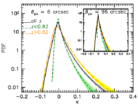
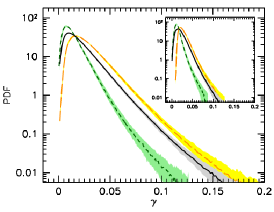
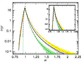
Figure 14: Same as Fig. 13 for maps extracted from the light-cones considering a CFHTLS-like source redshift distribution, considering the original maps with $\theta_{pix}=6$ arcsec. While the black curves show the median of the total source sample, the long-dashed orange and the short-dashed green refer to sources above and below the median source redshift $\langle z\rangle$=0.87, respectively. Shaded regions enclose the first and the third quartile of the distributions at fixed value. The small sub-panels show the same distributions from the maps with $\theta_{pix}=96$ arcsec, corresponding to scale at which the different source redshift maps in the light-cone are not affected by particle shot-noise.

In Fig. 14 we show the median Probability Distribution Functions of convergence, shear and magnification combining different catalogues extracted from the 54 and 99 realisations of W1 and W4 – using the original maps with pixel size equal to $6$ arcsec, respectively. In particular for each field of view we generate 8 different random catalogues sampling the CFHTLS source redshift distribution and randomly locating the sources within the field of view for a total of 1224 catalogues. We do not account for any clustering in the source distribution since this is beyond the purpose of this first work. The black histograms display the case of the whole source sample up to redshift $z_{s}=2.3$, while the short dashed green and the long dashed orange refer to the lensing quantities computed for sources below and above the median value $z_{m}=0.87$, respectively. For each histogram the corresponding shaded regions enclose the first and the third quartile of the distributions at fixed value. The small sub panels show the distributions from the same source redshift distribution obtained from the maps degraded by a factor of $16$ with respect to the original ones. As we have noticed in the bottom panels of Fig. 13 in these case the distributions are less spread and miss of the values regime tails (Takahashi et al., 2011).

4.1 Other Statistics

In this section, we study the predictions for other lensing statistics from the simulated light-cones. Besides the power spectrum, there are other lensing statistics that can be used to probe both the small scale matter density distribution and the dark energy equation of state, as well as the power spectrum normalisation. Among these, the top-hat shear dispersion (equivalent to the variance of the convergence field convolved with a top-hat filter) and the aperture-mass dispersion (equivalent to the variance of the convergence field convolved with a compensated aperture filter) are the most widely used used for cosmological investigation. Comparisons with theoretical models can be easily done considering that these quantities can be analytically computed as weighted integrals of the convergence power spectrum.

The two filter that we will adopt to convolve the convergence maps are:

$$\tilde{W}_{TH}=\dfrac{2J_{1}(l\theta)}{l\theta}$$ (22)

for the top-hat shear dispersion and

$$\tilde{W}_{Ap}=\dfrac{\sqrt{276}J_{4}(l\theta)}{(l\theta)^{2}}$$ (23)

for the aperture-mass dispersion. The functions $J_{1}(x)$ and $J_{4}(x)$ represent the first and the forth order Bessel functions, respectively. To clarify our methodology, in the the first case we will compute the second-order statistics from the following relation:

$$\langle\kappa^{2}\rangle_{TH/Ap}=\dfrac{1}{2\pi}\int\mathrm{d}l\,lP_{\kappa}(l)\tilde{W}^{2}_{TH/Ap}(l\theta)\,;$$ (24)

considering the appropriate weight function in each case and using the $P_{\kappa}(l)$ computed from the convergence maps.

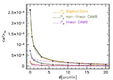
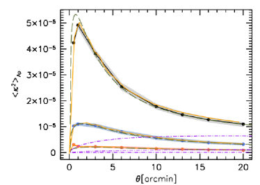
Figure 15: Variance of the convergence field in a top-hat (left) and in a compensated aperture (right) computed averaging over all the light-cone realisations. The various line styles refer to three different source redshifts considered $z=2.3$, 1 and 0.5: solid, dashed and long-dashed, respectively. The shaded regions represent the variance of the measurements in all realisations. The orange solid curves show the predictions computed from the convergence power spectrum at the corresponding redshifts.

These statistics can be calculated by either applying the filter to the two dimensional convergence field and then finding the variance or by finding the power spectrum of the field and then doing the integrals above, the latter being much faster on large fields. It is possible that numerical effects could make these results different in practice. As a cross-check we calculated them in both ways and find they are in very good agreement as will be seen in the plots.

In Fig. 15 we show the top-hat shear (left) and the aperture-mass dispersion (right) as measured in the different realisations of the two considered light-cones with sources at redshift $z_{s}=0.5$, 1 and 2.3 – the corresponding redshift colours have been chosen as in Fig. 13. The coloured lines connecting the data points show the median measurements from the maps, at each corresponding redshift, with the corresponding shaded regions enclosing the first and the third quartile on the different realisations – slow computation. We remind the reader that aperture-mass dispersion data for $z_{s}=0.5$ and $\theta\lesssim 1.6$ arcmin may be affected by particle shot-noise. From the other side small scale particle shot-noise does not appear for the measurements for $z_{s}=1$ and $2.3$.

The solid orange curves, instead, display the measurements done adopting the computed convergence power spectra from the maps in equation (24). The dashed green and the dot-dashed magenta curves show the predictions – from equation (24) – adopting linear and non-linear power spectra as implemented in CAMB. Apart for the linear case, all the measurements are in quite good agreement with each other, indicating the importance of non-linear modelling on the small scale lensing measurements. In the case of a top-hat filter the differences between the linear and nonlinear results start to be significant on scales below $\sim 5-7$ arcmin – depending on the source redshifts, for the compensated aperture the deviations are already evident at 20 arcmin. These behaviours are related to the relative weighs assigned to different scales by the two considered filters. In particular, the compensated aperture filter is very peaked enhancing the non-linearities of the matter density distribution at larger $\theta$ (Schneider et al., 1998).

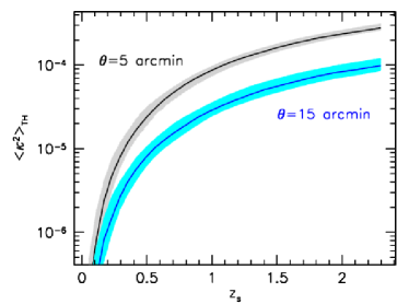
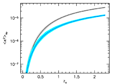
Figure 16: Median variance in a top-hat (left) and in a compensated aperture (right) of the convergence maps as a function of the source redshifts for two different smoothing scales: $\theta=5$ and $15$ arcmin. The curves represent the median of the measurements as performed from the different simulated lensing maps and the shaded regions enclose the first and the third quartile of the distribution at fixed source redshift.

Despite the close agreement between analytic theory and the simulations there are differences which can be seen in Fig.  15. They are most pronounced in the right hand panel, for the aperture-mass dispersion, at small smoothing scale filters and for $z_{s}=2.3$. This discrepancy was also noticed at high redshift in the 3D matter power spectrum as presented in Fig. 1.

For sources at higher redshift the fluctuations in the convergence are larger. As shown in Fig. 16 both the top-hat shear rms and the aperture mass dispersion grow by about two orders of magnitude between a source redshift of $z_{s}=0.2$ and $z_{s}=2$. In the figure we present the median measurement for two filtering scales $\theta=5$ and 15 arcmin – representing the typical scales enclosing the central region of a galaxy cluster; where we notice that for smaller $\theta$ the difference of the non-linear contributions between low and high redshifts structures is more enhanced than for larger filters.

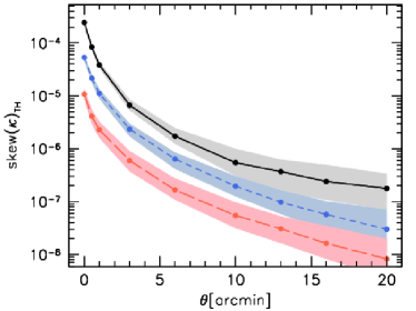
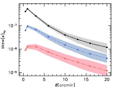
Figure 17: Skewness of the filtered convergence maps with a top-hat (left) and an aperture (right) function measured on all the light-cone realisations as a function of the smoothing scale $\theta$. The different line styles refer to three different source redshifts considered $z=2.3$, 1 and 0.5: solid, dashed and long-dashed, respectively.

Another important probe for understanding the small scale clustering of dark matter and evolution of dark energy evolution are the three point statistics. We compute the skewness of the convergence maps for each light cone realisation both for W1 and W4, for different source redshifts and filtering scales $\theta$ computing:

$$\mathrm{skew}(\kappa)_{TH/Ap}=\dfrac{\langle\kappa^{3}\rangle_{TH/Ap}}{\langle\kappa^{2}\rangle^{3/2}_{TH/Ap}}=\dfrac{\dfrac{1}{n-1}\sum_{i}\left(\tilde{\kappa}_{i}-\langle\tilde{\kappa}\rangle\right)^{3}}{\left[\dfrac{1}{n-1}\sum_{i}\left(\tilde{\kappa}_{i}-\langle\tilde{\kappa}\rangle\right)^{2}\right]^{3/2}}$$ (25)

where the sum is extended up to $n$, equals to the total number of pixels in each map and $\tilde{k}$ represent the filtered converge map. As done previously, we adopt both the top-hat and the compensated aperture filter. In Fig. 17 we show the median of the skewness for three different source redshifts both for the top-hat (left) and the compensated aperture filter (right). Black, blue and red show the cases for sources at redshift $z_{s}=2.3$, 1 and $0.5$, with the corresponding shaded regions enclosing the first and the third quartile of the distribution. The redshift evolution of the skewness, for the two filters, is shown in Fig. 18 again for $\theta=5$ (black) and $15$ arcmin (blue).

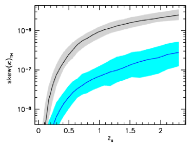
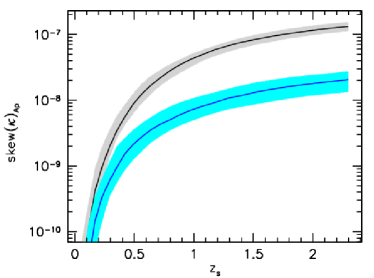
Figure 18: Median skewness in a top-hat (left) and in a compensated aperture (right) of the convergence maps as a function of the source redshifts for two different smoothing scales: $\theta=5$ (higher) and $15$ arcmin (lower).

The last statistic that we address in this section regards the noise from large scale structures to the average tangential shear in a thin circular annuls. This quantity is important to understand the noise induced by uncorrelated structure along the line-of-sight when measuring the tangential shear profile of a galaxy cluster and the accuracy with which its mass and concentration can be recovered (Hoekstra et al., 2011; Giocoli et al., 2014; Petkova et al., 2014). Typically this noise depends on the scale we are looking at and so tends to be different in the weak and the strong lensing regions of a galaxy cluster. While the strong lensing signal appears toward the core of the galaxy cluster, typically scales well below an arcminute, the weak lensing signal extends out to larger scales – from some arcminutes and above. In order to compute this noise from our simulated light-cones we adopt the formalism as presented by Hoekstra (2003) where the convergence field is convolved with the following filtering function in Fourier space:

$$g(l\theta)=\dfrac{J_{2}(l\theta)}{2\pi}\,,$$ (26)

where $J_{2}$ represents the second order Bessel function. The noise from Large Scale Structures (LSS) $\sigma_{LSS}$ will be given by the square root of the variance of the convergence field convolved with $g(l\theta)$. We do this for each realisation of the W1 and the W4 fields and each considered source redshift (see Fig. 4). In Fig. 19 we present the median noise by LSS as a function of the source redshifts for different filtering scales $\theta$. At fixed redshift the noise decreases as a function of $\theta$ and it increases as a function of the source redshift for fixed $\theta$. In the figure we notice also that the measurements for $\theta=0.5$ arcmin at for $z_{s}<0.75$ present a hump due to the discreetness of the particle density distribution in the simulation.

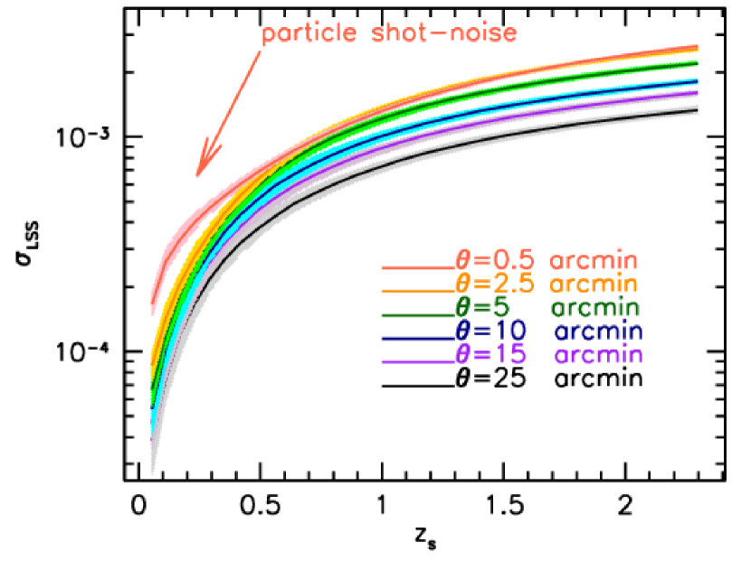
Figure 19: Large scale structure noise in the spherical averaged shear profile as a function of the source redshift and for different filtering scales.

From the figure we can see that from low ($z_{s}$=0.2) to high ($z_{s}=2$) redshift sources the noise in the spherical averaged shear profile increases by approximately one orders of magnitudes.

4.2 Halo-shear lensing signal

We study in this section the cross-correlation signal between halo positions and the surrounding density. For this, we identify dark matter halos and remap their positions into cuboidal coordinates similarly as previously done with the particle density in building up the light-cones. We then compute the halo-shear lensing cross-correlation in comoving coordinates as:

$$\Delta\Sigma(r_{p})=\gamma_{t}(r_{p})\Sigma_{\rm crit},$$ (27)

from the shear catalogs of background source galaxies surrounding each halo centres in projection. To account for the different mass over-density distributions, we divide halos into five mass bins ranging from $10^{12}$ to $10^{15}$ $h^{-1}\rm{M_{\odot}}$. We also compute $\Delta\Sigma(r_{p})$ directly from the projected density map by stacking the particle density around the same halos. The averaged $\Delta\Sigma(r_{p})$ among the various light-cone realisations are shown in Figure 20 and Figure 21 for $z=0.52$ and $z=0.8$ respectively. Error bars correspond to standard deviations among light-cone realisations. These signals are compared with halo model predictions. For the latter, we used the detailed prescription presented in van den Bosch et al. (2013), which accurately includes the halo exclusion effect (in computing the two halo term two haloes cannot be less distant than the sum of their virial radii): distinct haloes. In the model, we assumed NFW halo radial density profiles with a concentration-mass relation as consistently computed by Prada et al. (2012) and used the halo mass and bias functions by Tinker et al. (2010).

First, we found that our cross-correlation and stacking measurements are in good agreement, meaning that our lensing procedure does not introduce any significant noise or smoothing. Second, we found a good agreement with theory on large scale, but some discrepancies on small scale. The dependence of the discrepancies on the halo mass is due to the density contrast estimator $\Delta\Sigma$ applied on the actual density profile $\Sigma(R)$. The amplitude of the discrepancy depends on the map resolution but also on the steepness of the density profile above the background (i.e. the 2-halo term). For the high mass halos, the steep NFW tail is above the background over a large radial range, whereas for the low mass halos, the profile is buried in the background for the most part, and only the inner and shallower part can be distinguished from the background. At very small scale, where the density signal $\Sigma(R)$ in the maps is not properly resolved, the measured density contrast $\Delta\Sigma(R)$ drops. We performed a test by degrading the map by a factor of 4 and observed that the discrepancies were shifted to larger radii in agreement with this explanation.

At redshift $z=0.52$, the difference between the stacking and the cross-correlation measurements is due to the shot noise in the maps, which increases at lower redshift. We also have quantified the impact of shear versus reduced-shear measurements, but at these scales there is no differences even for the highest halo-mass bins. In summary, the discrepancies between theoretical and measured curves in figures 20 and 21 at small angular separation are consistent with numerical resolution limitations.

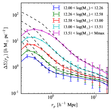
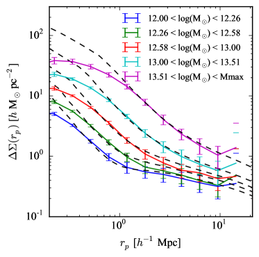
Figure 20: (left) Halo-galaxy lensing signal measured for halos in different mass bins at redshift $z=0.52$ in field W1. Theoretical predictions are shown in dashed lines. (right) Projected density contrast profile obtained by stacking the density field around halos of the same mass bin. Distances and densities are computed in comoving coordinates to ease the comparison with the halo model predictions.

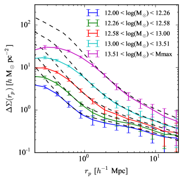
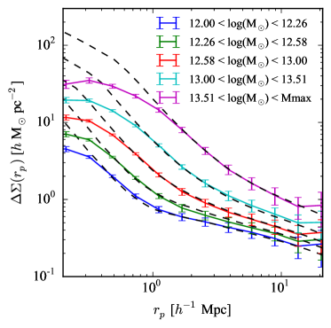
Figure 21: Same as Figure 20 but at redshift $z=0.8$.

5 Summary and Conclusion

In the context of forthcoming large spectroscopic and imaging wide field surveys that aim at high-precision cosmology, it is mandatory to have precise numerical simulations in order to test the methods of analysis, evaluate their predictive power, and estimate errors in the observables.

In this paper, we present the simulations that we are using in several forthcoming papers in which we cross-correlate weak lensing and other observables. The produced light-cones are extracted from the $(2.5\ \mathrm{Gpc}/h)^{3}$ BigMDPL cosmological simulation. They have been designed so that they match the shape of the publicly available VIPERS fields W1 and W4, and cover all redshifts up to $z=2.3$. In total, we produced 845 deg², and 871 deg² of independent light-cone realisations for W1 and W4 respectively. All of them include both lensing and halo mock catalogs with masses $M_{200}>10^{12}M\odot/h$.

We have performed several tests including cosmic shear 2-points and 3-points statistics, as well as halo-galaxy lensing test for different bins of mass and redshifts, and we found good agreement with theoretical predictions down to the scales numerically resolved by the BigMDPL simulation. In particular, the converge power spectra have also been compared with the analytic predictions from CAMB finding small departures well below $5\%$ for all the considered source redshifts, that should be taken into account in future modelling for the coming area of precision cosmology.

We provide a first release of the lensing and halo mock catalogs on the Bologna Lens Factory web site . Tools and particular statistics are also available upon request as well as lensing catalogs for specific source redshift distribution.

References

- Bartelmann & Schneider (2001) Bartelmann M., Schneider P., 2001, Physics Reports, 340, 291
- Carlson & White (2010) Carlson J., White M., 2010, ApJS, 190, 311
- Cooray & Hu (2001) Cooray A., Hu W., 2001, ApJ, 554, 56
- Flaugher (2005) Flaugher B., 2005, International Journal of Modern Physics A, 20, 3121
- Giocoli et al. (2014) Giocoli C., Meneghetti M., Metcalf R. B., Ettori S., Moscardini L., 2014, MNRAS, 440, 1899
- Giocoli et al. (2015) Giocoli C., Metcalf R. B., Baldi M., Meneghetti M., Moscardini L., Petkova M., 2015, MNRAS, 452, 2757
- Guzzo et al. (2014) Guzzo L., Scodeggio M., Garilli B., Granett B. R., Fritz A., Abbas U., Adami C., Arnouts et al. 2014, A&A, 566, A108
- Harnois-Déraps et al. (2012) Harnois-Déraps J., Vafaei S., Van Waerbeke L., 2012, MNRAS, 426, 1262
- Hilbert et al. (2009) Hilbert S., Hartlap J., White S. D. M., Schneider P., 2009, A&A, 499, 31
- Hildebrandt et al. (2012) Hildebrandt H., Erben T., Kuijken K., van Waerbeke L., Heymans C., Coupon J., Benjamin J., et al. 2012, MNRAS, 421, 2355
- Hockney & Eastwood (1988) Hockney R. W., Eastwood J. W., 1988, Computer simulation using particles
- Hoekstra (2003) Hoekstra H., 2003, MNRAS, 339, 1155
- Hoekstra et al. (2011) Hoekstra H., Hartlap J., Hilbert S., van Uitert E., 2011, MNRAS, 412, 2095
- Ivezic et al. (2008) Ivezic Z., Tyson J. A., Abel B., Acosta E., Allsman R., AlSayyad Y., Anderson S. F., Andrew J., for the LSST Collaboration 2008, ArXiv e-prints
- Kaiser (1992) Kaiser N., 1992, ApJ, 388, 272
- Kaiser (1998) Kaiser N., 1998, ApJ, 498, 26
- Klypin & Holtzman (1997) Klypin A., Holtzman J., 1997, ArXiv Astrophysics e-prints
- Klypin et al. (2013) Klypin A., Prada F., Yepes G., Hess S., Gottlober S., 2013, ArXiv e-prints
- Klypin et al. (2014) Klypin A., Yepes G., Gottlober S., Prada F., Hess S., 2014, ArXiv e-prints
- Laureijs et al. (2011) Laureijs R., Amiaux J., Arduini S., Auguères J. ., Brinchmann J., Cole R., Cropper M., Dabin C., Duvet L., et al. 2011, ArXiv e-prints
- Lewis et al. (2000) Lewis A., Challinor A., Lasenby A., 2000, Astrophys. J., 538, 473
- Metcalf & Petkova (2014) Metcalf R. B., Petkova M., 2014, MNRAS, 445, 1942
- Pace et al. (2015) Pace F., Baldi M., Moscardini L., Bacon D., Crittenden R., 2015, MNRAS, 447, 858
- Petkova et al. (2014) Petkova M., Metcalf R. B., Giocoli C., 2014, MNRAS, 445, 1954
- Planck Collaboration et al. (2013) Planck Collaboration Ade P. A. R., Aghanim N., Armitage-Caplan C., Arnaud M., Ashdown M., Atrio-Barandela F., Aumont J., Baccigalupi C., Banday A. J., et al. 2013, ArXiv e-prints
- Prada et al. (2012) Prada F., Klypin A. A., Cuesta A. J., Betancort-Rijo J. E., Primack J., 2012, MNRAS, 423, 3018
- Prada et al. (2014) Prada F., Scoccola C. G., Chuang C.-H., Yepes G., Klypin A. A., Kitaura F.-S., Gottlober S., 2014, ArXiv e-prints
- Riebe et al. (2013) Riebe K., Partl A. M., Enke H., Forero-Romero J., Gottlöber S., Klypin A., Lemson G., Prada F., Primack J. R., Steinmetz M., Turchaninov V., 2013, Astronomische Nachrichten, 334, 691
- Rodriguez et al. (2015) Rodriguez F., Merchán M., Sgró M. A., 2015, A&A, 580, A86
- Sato & Nishimichi (2013) Sato M., Nishimichi T., 2013, Phys.Rev.D, 87, 123538
- Schäfer et al. (2012) Schäfer B. M., Heisenberg L., Kalovidouris A. F., Bacon D. J., 2012, MNRAS, 420, 455
- Schneider (1996) Schneider P., 1996, MNRAS, 283, 837
- Schneider et al. (1998) Schneider P., van Waerbeke L., Jain B., Kruse G., 1998, MNRAS, 296, 873
- Schneider et al. (2002) Schneider P., van Waerbeke L., Kilbinger M., Mellier Y., 2002, A&A, 396, 1
- Scoccimarro et al. (1999) Scoccimarro R., Zaldarriaga M., Hui L., 1999, ApJ, 527, 1
- Smith et al. (2003) Smith R. E., Peacock J. A., Jenkins A., White S. D. M., Frenk C. S., Pearce F. R., Thomas P. A., Efstathiou G., Couchman H. M. P., 2003, MNRAS, 341, 1311
- Spergel et al. (2013) Spergel D., Gehrels N., Breckinridge J., Donahue M., Dressler A., Gaudi B. S., Greene T., Guyon O., Hirata C., et al. K., 2013, arXiv:1305.5422
- Takahashi et al. (2011) Takahashi R., Oguri M., Sato M., Hamana T., 2011, ApJ, 742, 15
- Takahashi et al. (2012) Takahashi R., Sato M., Nishimichi T., Taruya A., Oguri M., 2012, ApJ, 761, 152
- The Dark Energy Survey Collaboration (2005) The Dark Energy Survey Collaboration 2005, ArXiv Astrophysics e-prints
- Tinker et al. (2010) Tinker J. L., Robertson B. E., Kravtsov A. V., Klypin A., Warren M. S., Yepes G., Gottlöber S., 2010, ApJ, 724, 878
- Vale & White (2003) Vale C., White M., 2003, ApJ, 592, 699
- van den Bosch et al. (2013) van den Bosch F. C., More S., Cacciato M., Mo H., Yang X., 2013, MNRAS, 430, 725