Electroweak top-quark pair production at the LHC with $Z^{\prime}$ bosons to NLO QCD in POWHEG

Abstract

We present the calculation of the NLO QCD corrections to the electroweak production of top-antitop pairs at the CERN LHC in the presence of a new neutral gauge boson. The corrections are implemented in the parton shower Monte Carlo program POWHEG. Standard Model (SM) and new physics interference effects are properly taken into account. QED singularities, first appearing at this order, are consistently subtracted. Numerical results are presented for SM and $Z^{\prime}$ total cross sections and distributions in invariant mass, transverse momentum, azimuthal angle and rapidity of the top-quark pair. The remaining theoretical uncertainty from scale and PDF variations is estimated, and the potential of the charge asymmetry to distinguish between new physics models is investigated for the Sequential SM and a leptophobic topcolor model.

1 Introduction

The Standard Model (SM) of particle physics is a very successful theory describing a wealth of experimental data up to collision energies of 13 TeV reached at CERN’s Large Hadron Collider (LHC). This includes the recent observation of a Higgs-like particle with a mass of 125 GeV that seems to corroborate the simplest description of electroweak symmetry breaking Aad:2012tfa ; Chatrchyan:2012ufa ; Aad:2015zhl . However, the SM is based on the unintuitive semi-simple gauge group SU(3)${}_{C}\times$SU(2)${}_{L}\times$U(1)_Y, that together with the running behavior of the associated gauge couplings intriguingly points towards a larger unification at some higher mass scale. The simple gauge group SU(5) can accomodate the complete SM gauge group and its 15 fermions, but not a right-handed neutrino, and it is in addition strongly disfavored by searches for proton decay. It also does not allow to restore parity symmetry and does not provide a natural solution to the neutrino mass hierarchy. Both of these important and perhaps related problems are solved in simple gauge groups of higher rank like $E_{6}$ or SO(10), that can be broken consecutively as in $E_{6}\to$SO(10)$\times$U(1)_ψ and SO(10)$\to$SU(5)$\times$U(1)_χ, respectively. Parity restoration is achieved in left-right symmetric models, SU(3)${}_{C}\times$SU(2)${}_{L}\times$SU(2)${}_{R}\times$U(1)_Y, which together with other models of similar group structure, but different quantum number assignments form a class of general lower-scale models, commonly called $G(221)$ models. They have recently been classified Hsieh:2010zr , and their phenomenology has been studied not only at the LHC Jezo:2012rm ; Jezo:2014wra ; Jezo:2015rha , but also in ultrahigh-energy cosmic rays Jezo:2014kla . Common to all these possible extensions of the SM is their prediction of a new heavy neutral gauge boson ($Z^{\prime}$), that is associated with the additional SU(2) or U(1) subgroup after symmetry breaking Langacker:2008yv ; Agashe:2014kda . In many cases, the $Z^{\prime}$ boson can decay leptonically, making it a prime object of experimental searches at the LHC. For simplification, these searches are mostly based on the (theoretically unmotivated) Sequential SM (SSM), where the $Z^{\prime}$ boson couples to other SM particles like the SM $Z$ boson. In this model and the leptonic (i.e. Drell-Yan) channel, the ATLAS and CMS collaborations have already excluded $Z^{\prime}$ bosons with masses below 2.90 TeV Aad:2014cka and 2.96 TeV CMS:2013qca , respectively. For a recent overview of experimental mass limits see Ref. Jezo:2014wra , where it is also shown that for certain $G(221)$ models the mass limits are enhanced to 3.2-4.0 TeV, when higher-order QCD corrections are included.

In this paper, we focus not only on the SSM, but also on a situation where the $Z^{\prime}$ boson does not couple to leptons, but preferentially to top quarks, so that the above mass limits are invalidated. Models of the $G(221)$ class, where processes of the Drell-Yan type are inaccessible at the LHC, include leptophobic (LP), hadrophobic (HP) and fermiophobic (FP) models, whereas left-right (LR), un-unified (UU) and non-universal (NU) models remain accessible. The LP model with a $W^{\prime}$-boson mass of about 2 TeV has been put forward as a possible explanation for the excesses of $WZ$ and $Wh$ production observed recently by ATLAS and CMS at the LHC Gao:2015irw . As the heaviest particle in the SM with a mass of 173 GeV ATLAS:2014wva , the top quark may very well play a special role in electroweak symmetry breaking. This motivates, e.g., the NU model, where the first and second SU(2) gauge groups couple exclusively to the first/second and third generation fermions, respectively. It also motivates models with new strong dynamics such as the topcolor model Hill:1991at ; Hill:1994hp , which can generate a large top-quark mass through the formation of a top-quark condensate. This is achieved by introducing a second strong SU(3) gauge group which couples preferentially to the third generation, while the original SU(3) gauge group couples only to the first and second generations. To block the formation of a bottom-quark condensate, a new U(1) gauge group and associated $Z^{\prime}$ boson are introduced. Different couplings of the $Z^{\prime}$ boson to the three fermion generations then define different variants of the model Harris:1999ya . A popular choice with the LHC collaborations is the leptophobic topcolor model (also called Model IV in the reference cited above) Harris:2011ez , where the $Z^{\prime}$ couples only to the first and third generations of quarks and has no significant couplings to leptons, but an experimentally accessible cross section.

The strongest limits on $Z^{\prime}$ bosons arise of course from their Drell-Yan like decays into electrons and muons at the LHC. This is due to the easily identifiable experimental signatures Jezo:2014wra . The top-pair signature is more difficult, as top quarks decay to $W$ bosons and bottom quarks, where the latter must be tagged and the two $W$ bosons may decay hadronically, i.e. to jets, or leptonically, i.e. into electrons or muons and missing energy carried away by a neutrino. In addition and in contrast to the Drell-Yan process, the electroweak top-pair production cross section obtains QCD corrections not only in the initial, but also in the final state. For conclusive analyses, precision calculations are therefore extremely important to reduce theoretical uncertainties, arising from variations of the renormalization and factorization scales $\mu_{r}$ and $\mu_{f}$ and of the parton density functions (PDFs) $f_{a/p}(x_{a},\mu_{f})$, and for an accurate description of the possible experimental signal and the SM backgrounds.

At the LHC, the hadronic top-pair production cross section

$$\sigma = \sum_{ab}\int f_{a/p}(x_{a},\mu_{f})f_{b/p}(x_{b},\mu_{f})\,{d\sigma_{ab}\over dt}(\mu_{r})\,dt\,dx_{a}dx_{b}$$ (1)

obtains up to next-to-leading order (NLO) the contributions

$$\sigma_{ab}(\mu_{r}) = \sigma_{2;0}(\alpha_{S}^{2})+{\color[rgb]{1,0,0}\sigma_{0;2}(\alpha^{2})}+\sigma_{3;0}(\alpha_{S}^{3})+\sigma_{2;1}(\alpha_{S}^{2}\alpha)+{\color[rgb]{1,0,0}\sigma_{1;2}(\alpha_{S}\alpha^{2})}+\sigma_{0;3}(\alpha^{3})\,,$$ (2)

where the numerical indices represent the powers of the strong coupling $\alpha_{S}(\mu_{r})$ and of the electromagnetic coupling $\alpha$, respectively. The first and third terms representing the SM QCD background processes $q\bar{q},gg\to t\bar{t}$ and their NLO QCD corrections, including the $qg$ channel, have been computed in the late 1980 Nason:1987xz ; Nason:1989zy ; Beenakker:1988bq ; Beenakker:1990maa . Furthermore, NLO predictions for heavy quark correlations have been presented in Mangano:1991jk , and the spin correlations between the top quark and antiquark have been studied in the early 2000s Bernreuther:2001rq ; Bernreuther:2004jv . The fourth term represents the electroweak corrections to the QCD backgrounds, for which a gauge-invariant subset was first investigated neglecting the interferences between QCD and electroweak interactions arising from box-diagram topologies and pure photonic contributions Beenakker:1993yr and later including also additional Higgs boson contributions arising in 2-Higgs doublet models (2HDMs) Kao:1999kj . The rest of the electroweak corrections was calculated in a subsequent series of papers and included also $Z$-gluon interference effects and QED corrections with real and virtual photons Kuhn:2005it ; Moretti:2006nf ; Bernreuther:2005is ; Bernreuther:2006vg ; Hollik:2007sw . In this paper, we focus on the second and fifth terms in Eq. (2) (highlighted in red), i.e. the contribution $\sigma_{0;2}$ for the $Z^{\prime}$ signal and its interferences with the photon and SM $Z$ boson and the corresponding QCD corrections $\sigma_{1;2}$. Due to the resonance of the $Z^{\prime}$ boson, we expect these terms to be the most relevant for new physics searches. A particular advantage of this choice is that the calculation of $\sigma_{1;2}$ can then be carried out in a model-independent way as long as the $Z^{\prime}$ couplings are kept general, whereas the fourth term $\sigma_{2;1}$ is highly model-dependent due to the rich structure of the scalar sector in many models. The sixth term in Eq. (2) is suppressed by a relative factor $\alpha/\alpha_{s}$ with respect to the fifth and thus small.

The production of $Z^{\prime}$ bosons (and Kaluza-Klein gravitons) decaying to top pairs has been computed previously in NLO QCD by Gao et al. in a factorized approach, i.e. neglecting all SM interferences and quark-gluon initiated diagrams with the $Z^{\prime}$ boson in the $t$-channel, and for purely vector- and/or axial-vector-like couplings as those of the SSM Gao:2010bb . We have verified that we can reproduce their $K$-factors (i.e. the ratio of NLO over LO predictions) of 1.2 to 1.4 (depending on the $Z^{\prime}$ mass) up to 2%, if we reduce our calculation to their theoretical set-up and employ their input parameters. Their result has triggered the Tevatron and LHC collaborations to routinely use a $K$-factor of 1.3 in their experimental analyses (see below). The factorized calculation by Gao et al. has been confirmed previously in an independent NLO QCD calculation by Caola et al. Caola:2012rs . Like us, these last authors include also the additional quark-gluon initiated processes and show that after kinematic cuts they reduce the $K$-factor by about 5 %. However, they still do not include the additional SM interferences, which they claim to be small for large $Z^{\prime}$-boson masses. As we will show, this is not always true due to logarithmically enhanced QED contributions from initial photons. In contrast to us, they also include top-quark decays in the narrow-width approximation with spin correlations and box-diagram corrections to interferences of the electroweak and QCD Born processes ($\sigma_{2;1}$ in Eq. (2)), which are, however, only relevant for very broad resonances. If the (factorizable) QCD corrections to the top-quark decay are included, the $K$-factor is reduced by an additional 15%. The globally smaller $K$-factor of Caola et al. is thus explained by calculational aspects and not by different choices of input parameters.

The SM backgrounds are today routinely calculated not just in NLO QCD, but at NLO combined with parton showers (PS), e.g. within the framework of MC@NLO or POWHEG Frixione:2002ik ; Frixione:2007vw . A particularly useful tool is the POWHEG BOX, in which new processes can be implemented once the spin- and color-correlated Born amplitudes along with their virtual and real NLO QCD corrections are known and where the regions of singular radiation are then automatically determined Alioli:2010xd . Calculations of this type have already been performed by us in the past for the Drell-Yan like production of $Z^{\prime}$ bosons Fuks:2007gk , heavy-quark production in the ALICE experiment Klasen:2014dba , and the associated production of top quarks and charged Higgs bosons Weydert:2009vr ; Klasen:2012wq . In this work, we provide a calculation of the $Z^{\prime}$ signal with a final top-quark pair at the same level of accuracy, including all interferences with SM $Z$ bosons and photons as well as the logarithmically enhanced QED contributions from initial-state photons, which we will discuss in some detail. We also present details about the spin- and color-correlated Born amplitudes, the treatment of $\gamma_{5}$ and renormalization procedure in our calculation of the virtual corrections, as well as the validation of our NLO+PS calculation, which we have performed with the calculation for $Z^{\prime}$ bosons of Gao et al. at NLO Gao:2010bb and for tree-level and one-loop SM matrix elements with MadGraph5_aMC@NLO Alwall:2014hca and GoSam Cullen:2011ac .

Experimental searches for resonant top-antitop production have been performed at the Tevatron and at the LHC mostly for the leptophobic topcolor model with a $Z^{\prime}$-boson coupling only to first and third generation quarks Harris:1999ya ; Harris:2011ez . In this model, the LO cross section is controlled by three parameters: the ratio of the two U(1) coupling constants, $\cot\theta_{H}$, which should be large to enhance the condensation of top quarks, but not bottom quarks, and which also controls both the $Z^{\prime}$ production cross section and decay width, as well as the relative strengths $f_{1}$ and $f_{2}$ of the couplings of right-handed up- and down-type quarks with respect to those of the left-handed quarks. The LO cross sections for this model are usually computed for a fixed small $Z^{\prime}$ width, $\Gamma_{Z^{\prime}}=1.2\%\times m_{Z^{\prime}}$, effectively setting the parameter $\cot\theta_{H}$, and the choices $f_{1}=1$, $f_{2}=0$, which maximize the fraction of $Z^{\prime}$ bosons that decay into top-quark pairs. We have verified that we can reproduce the LO numerical results in the paper by Harris and Jain Harris:2011ez for $Z^{\prime}$ masses above 1 TeV and relative widths of 1% and 1.2%, but not 10%, if we neglect all SM interferences. As stated above, the LO cross sections are routinely multiplied by the experimental collaborations by a $K$-factor of 1.3 Gao:2015irw . At the Tevatron with center-of-mass energy $\sqrt{S}=1.96$ TeV and in the lepton+jets top-quark decay channel, CDF and D0 exclude $Z^{\prime}$ bosons with masses up to 0.915 TeV Aaltonen:2012af and 0.835 TeV Abazov:2011gv , respectively. The weaker D0 limit can be explained by the fact that CDF use the full integrated luminosity of 9.45 fb^-1, while D0 analyze only 5.3 fb^-1 and furthermore do not use a $K$-factor for the signal cross section. At the LHC, the ATLAS and CMS collaborations have analyzed 20.3 fb^-1 and 19.7 fb^-1 of integrated luminosity of the $\sqrt{S}=8$ TeV LHC run employing the $K$-factor of 1.3. The result is that narrow leptophobic topcolor $Z^{\prime}$ bosons are excluded below masses of 1.8 TeV and 2.4 TeV, respectively Aad:2015fna ; Khachatryan:2015sma . At the LHC, the CMS limit is currently considerably stronger than the one by ATLAS despite the slightly smaller exploited luminosity. The reason is that CMS performed a combined analysis of all top-quark decay channels (dilepton, lepton+jets and all hadronic), while ATLAS analyzed only the lepton+jets channel. For $\Gamma_{Z^{\prime}}=10\%\times m_{Z^{\prime}}$, the CMS mass limit is even stronger and is found to be 2.9 TeV. We emphasize that the narrow width assumption employed in most experimental analyses need not be realized in nature and that in this case a proper treatment of SM interference terms as provided in our full calculation is required.

The LHC has just resumed running with an increased center-of-mass energy of 13 TeV, which is planned to be increased to 14 TeV in the near future. We therefore provide numerical predictions in this paper for both of these energies and for two benchmark models, i.e. the SSM and the leptophobic topcolor model. The predictions for the SSM are readily obtained by taking over the $Z^{\prime}$-boson couplings from the SM, with the consequence of again a relatively small width $\Gamma_{Z^{\prime}}\simeq 3\%\times m_{Z^{\prime}}$ for $Z^{\prime}$ masses between 3 and 6 TeV. We focus on the invariant-mass distribution of the top-quark pair, which is the main observable exploited for resonance (and in particular $Z^{\prime}$-boson) searches, but also show results for the distributions that are most sensitive to soft parton radiation beyond NLO, i.e. the transverse momentum $p_{t\bar{t}}$ of the top-antitop pair and their relative azimuthal angle $\phi_{t\bar{t}}$. The forward-backward asymmetry $A_{FB}$ of top-antitop events with positive vs. negative rapidity difference between the two has also been suggested as a very useful observable to distinguish among different models Kamenik:2011wt . At the Tevatron (a $p\bar{p}$ collider, where top quarks are produced predominantly in the direction of the proton beam), long-standing discrepancies of CDF and D0 measurements with the SM prediction at NLO Aaltonen:2011kc ; Abazov:2011rq have triggered numerous suggestions of new physics contributions Kamenik:2011wt , e.g. of light $Z^{\prime}$ bosons coupling in a flavor non-diagonal way to up and top quarks Buckley:2011vc . Only recently the SM prediction at next-to-next-to-leading order (NNLO) Czakon:2014xsa has been brought in agreement with the newest inclusive measurement by CDF Aaltonen:2012it and differential measurement by D0 Abazov:2014cca . At the LHC (a $pp$ collider), a charge asymmetry $A_{C}$ can be defined with respect to the difference in absolute value of the top and antitop rapidities AguilarSaavedra:2012rx . We therefore also provide numerical predictions for this observable in our two benchmark models and at current and future LHC center-of-mass energies.

Our paper is organized as follows: In Sec. 2 we present analytical results of our calculations at LO and the NLO virtual and real corrections, including details about SM interference terms, our treatment of $\gamma_{5}$, our renormalization procedure and the subtraction method employed for the soft and collinear divergences in the real corrections. In Sec. 3 we discuss the implementation of our calculation in POWHEG and present in particular the color- and spin-correlated Born amplitudes, the definition of the finite remainder of the virtual corrections, the implementation of the real corrections with a focus on the rather involved treatment of QED divergences, and the validation of our tree-level matrix elements in the SM against those of the automated tool MadGraph5_aMC@NLO Alwall:2014hca and of the virtual corrections against those of GoSam Cullen:2011ac as well as of our numerical pure $Z^{\prime}$-boson results against those obtained by Gao et al. and Caola et al. Our new numerical predictions for the LHC are shown and discussed in Sec. 4, and Sec. 5 contains our conclusions. Several technical details of our calculation can be found in the Appendix.

2 NLO QCD corrections to electroweak top-pair production

In this section, we present in detail our calculation of the NLO QCD corrections to electroweak top-pair production through photons, SM $Z$ bosons and additional $Z^{\prime}$ bosons with generic vector and axial-vector couplings to the SM fermions. We generate all Feynman diagrams automatically with QGRAF Nogueira:1991ex and translate them into amplitudes using DIANA Tentyukov:1999is . The traces of the summed and squared amplitudes with all interferences are then calculated in the Feynman gauge and $D=4-2\varepsilon$ dimensions in order to regularize the ultraviolet (UV) and infrared (IR) divergences using FORM Vermaseren:2000nd . Traces involving the Dirac matrix $\gamma_{5}$ are treated in the Larin prescription Larin:1993tq by replacing $\gamma_{\mu}\gamma_{5}=i\frac{1}{3!}\varepsilon_{\mu\nu\rho\sigma}\gamma^{\nu}\gamma^{\rho}\gamma^{\sigma}$. To restore the Ward identities and thus preserve gauge invariance at one loop, we perform an additional finite renormalization for vertices involving $\gamma_{5}$.

2.1 Leading-order contributions

The leading-order (LO) Feynman diagrams contributing to the electroweak production of top-quark pairs at ${\cal O}(\alpha)$ through photons, SM $Z$ bosons and new $Z^{\prime}$ bosons are shown summarily in Fig. 1.

Figure 1: Tree-level Feynman diagrams of order $\mathcal{O}(\alpha)$ contributing to electroweak top-pair production through vector bosons $V$, i.e. photons ($\gamma$), SM $Z$ bosons and new $Z^{\prime}$ bosons.

The cross section $d\sigma/dt$, differential in the Mandelstam variable $t$ denoting the squared momentum transfer, is then obtained by summing all three corresponding amplitudes, squaring them, summing/averaging them over final-/initial-state spins and colors and multiplying them with the flux factor $1/(2s)$ of the incoming and the differential phase space $1/(8\pi s)$ of the outgoing particles. The Mandelstam variable $s$ denotes the squared partonic center-of-mass energy. The result, given here for brevity only in four and not $D$ dimensions, is

$${d\sigma_{q\bar{q}}\over dt} = \frac{1}{2s}\frac{1}{8\pi s}{B}_{q\bar{q}}$$

$$= \frac{1}{2s}\frac{1}{8\pi s}\sum_{V,V^{\prime}}\frac{2e^{4}D_{V}D_{V^{\prime}}}{s_{W}^{4}}\left\{s(t-u)\left(A_{V}^{{q}}B_{V^{\prime}}^{{q}}+A_{V^{\prime}}^{{q}}B_{V}^{{q}}\right)\left(A_{V}^{{t}}B_{V^{\prime}}^{{t}}+A_{V^{\prime}}^{{t}}B_{V}^{{t}}\right)\right.$$

$$+ \left.\left(A_{V}^{{q}}A_{V^{\prime}}^{{q}}\!+\!B_{V}^{{q}}B_{V^{\prime}}^{{q}}\right)\left[\left(t^{2}+u^{2}+4sm_{{t}}^{2}-2m_{{t}}^{4}\right)A_{V}^{{t}}A_{V^{\prime}}^{{t}}+\left(t^{2}+u^{2}-2m_{{t}}^{4}\right)B_{V}^{{t}}B_{V^{\prime}}^{{t}}\right]\right\}$$

$$\times \left\{\left[(s\!-\!m_{V}^{2})(s\!-\!m_{V^{\prime}}^{2})+m_{V}m_{V^{\prime}}\Gamma_{V}\Gamma_{V^{\prime}}\right]+i\left[(s\!-\!m_{V}^{2})m_{V^{\prime}}\Gamma_{V^{\prime}}-(s\!-\!m_{V^{\prime}}^{2})m_{V}\Gamma_{V}\right]\right\},$$

where ${B}_{q\bar{q}}$ is the modulus squared of the Born amplitude averaged/summed over initial/final spins and colors, $V,V^{\prime}\in\{\gamma,Z,Z^{\prime}\}$, the superscript $q$ denotes the flavor of the incoming massless quarks, $s,\ t,\ u$ are the partonic Mandelstam variables, and $m_{t}$ is the top-quark mass. Note that we use the Pauli metric, in which the dot-product has an overall minus sign with respect to the Bjorken-Drell metric Veltman:1994wz . The terms $D_{V},D_{V^{\prime}}$ stem from the propagator denominators and take the usual form

$$D_{\gamma}=\frac{1}{s^{2}},\ D_{Z}=\frac{1}{(s-m_{Z}^{2})^{2}+m_{Z}^{2}\Gamma_{Z}^{2}},\ D_{Z^{\prime}}=\frac{1}{(s-m_{Z^{\prime}}^{2})^{2}+m_{Z^{\prime}}^{2}\Gamma_{Z^{\prime}}^{2}}\,.$$ (4)

To take into account the finite widths of the $Z$ and $Z^{\prime}$ bosons, we have introduced complex masses $m_{Z(Z^{\prime})}\rightarrow m_{Z(Z^{\prime})}-i\Gamma_{Z(Z^{\prime})}/2$ with the consequence that $m_{Z(Z^{\prime})}^{2}\to m_{Z(Z^{\prime})}^{2}-\Gamma^{2}_{Z(Z^{\prime})}/4$. The coefficients $A^{{q}}_{V(V^{\prime})},B^{{q}}_{V(V^{\prime})},A^{{t}}_{V(V^{\prime})},B^{{t}}_{V(V^{\prime})}$ are proportional to the axial ($A$) and vector ($B$) couplings of the various gauge bosons to the massless quarks (${q}=u,d,s,c,b$) and the top quark (${t}$),

$$A_{\gamma}^{q} =s_{W}Q_{q}, A_{\gamma}^{{t}} =s_{W}Q_{t}, B_{\gamma}^{q} =0, B_{\gamma}^{{t}} =0,$$

$$A_{Z}^{q} =\frac{a_{Z}^{q}}{4c_{W}}, A_{Z}^{{t}} =\frac{a_{Z}^{t}}{4c_{W}}, B_{Z}^{q} =\frac{b_{Z}^{q}}{4c_{W}}, B_{Z}^{{t}} =\frac{b_{Z}^{t}}{4c_{W}},$$

$$A_{Z^{\prime}}^{q} =\frac{a_{Z^{\prime}}^{q}}{4c_{W}}, A_{Z^{\prime}}^{{t}} =\frac{a_{Z^{\prime}}^{{t}}}{4c_{W}}, B_{Z^{\prime}}^{q} =\frac{b_{Z^{\prime}}^{q}}{4c_{W}}, B_{Z^{\prime}}^{{t}} =\frac{b_{Z^{\prime}}^{{t}}}{4c_{W}}\,,$$ (5)

where $s_{W}\,(c_{W})$ are the sine (cosine) of the weak mixing angle $\theta_{W}$, $Q_{q}$ is the fractional charge of quark flavor $q$, and $a_{V}^{q}$ and $b_{V}^{q}$ are the model-dependent vector and axial-vector couplings of the $Z$ and $Z^{\prime}$ bosons, e.g. $a_{Z}^{u}=1-8/3s_{W}^{2}$, $a_{Z}^{d}=4/3s_{W}^{2}-1$, $b_{Z}^{u}=1$, $b_{Z}^{d}=-1$ for all up- and down-type quarks in the SM. Although individual interference terms may contain imaginary parts, they cancel as expected after summation.

2.2 One-loop virtual corrections

The one-loop virtual corrections contributing to electroweak top-pair production at $\mathcal{O}(\alpha_{s}\alpha^{2})$ originate from the interferences among the one-loop diagrams shown in Fig. 2 with the tree-level diagrams in Fig. 1.

Figure 2: One-loop Feynman diagrams of order $\mathcal{O}(\alpha_{S}\alpha)$ contributing to electroweak top-pair production.

Note that one-loop electroweak corrections to the QCD process $q\bar{q}\to g^{*}\to t\bar{t}$ have zero interference with the electroweak diagrams in Fig. 1, since such contributions are proportional to the vanishing color trace $\mathrm{Tr}(T^{a})$. In particular, the interference term of the box diagram in Fig. 3 with the amplitudes

Figure 3: Example of a box diagram of $\mathcal{O}(\alpha_{S}\alpha)$ leading to a vanishing contribution. This diagram would, however, contribute to electroweak corrections to the QCD Born processes.

in Fig. 1 vanishes, whereas it would of course contribute at $\mathcal{O}(\alpha_{s}^{2}\alpha)$.

As already mentioned, the virtual amplitudes are regularized dimensionally. The appearing 30 distinct loop integrals are then reduced to a basis of three master integrals using integration-by parts identities Tkachov:1981wb ; Chetyrkin:1981qh in the form of the Laporta algorithm Laporta:2001dd as implemented in the public tool REDUZE 2010CoPhC.181.1293S ; vonManteuffel:2012np . One is thus left with the evaluation of three master integrals: the massive tadpole, the equal-masses two-point function, and the massless two-point function. The solutions of these integrals are well known Hooft:1978xw . For completeness, we provide their analytic expressions in App. A.

In dimensional regularization, the UV and IR singularities in the virtual corrections appear as poles of $1/\varepsilon$ and $1/\varepsilon^{2}$. Since neither the couplings nor the top-quark mass have to be renormalized at NLO, the UV singularities can be removed by simply adding the Born cross section multiplied with the quark wave-function renormalization constants

$$\sum_{\psi\in\{{q},\bar{q},{t},\bar{t}\}}\frac{1}{2}\delta Z_{\psi}\,.$$ (6)

We use the on-shell renormalization scheme, in which $\delta Z_{q}=0$ for the initial-state massless quarks and

$$\delta Z_{t}=(4\pi)^{\varepsilon}\Gamma(1+\varepsilon)\left({\mu_{r}^{2}\over m_{t}^{2}}\right)^{\varepsilon}{C_{F}\alpha_{s}\over\pi}\left(-{3\over 4\varepsilon}-{1\over 1-2\varepsilon}\right)$$ (7)

for the final-state top quarks. Since we are using the Larin prescription for $\gamma_{5}$ (see above), we must perform an additional finite renormalization to restore the Ward identities. The corresponding constant has been calculated up to three loops in the $\overline{\mathrm{MS}}$ scheme Larin:1993tq . At one loop, it reads

$$\delta Z_{5}=-{C_{F}\alpha_{s}\over\pi}$$ (8)

and multiplies all appearing factors of $\gamma_{5}$. Once the UV divergences are renormalized, we are left with infrared collinear and soft divergences that match the correct structure given for instance in Refs. Catani:2002hc ; Frixione:1995ms . For completeness, we provide the analytic expressions of the IR poles in App. B.

2.3 Real emission corrections

At $\mathcal{O}(\alpha_{S}\alpha^{2})$, the following $2\rightarrow 3$ tree-level processes contribute: (i) $q+\bar{q}\to t+\bar{t}+g$and (ii) $g+q(\bar{q})\to t+\bar{t}+q(\bar{q})$. The corresponding Feynman diagrams are depicted in Figs. 4 and 5.

Figure 4: Diagrams contributing to the $q+\bar{q}\to t+\bar{t}+g$ subprocess at $\mathcal{O}(\alpha_{S}\alpha^{2})$ with $V\in\{\gamma,Z,Z^{\prime}\}$.

Figure 5: Diagrams contributing to the $g+q\to t+\bar{t}+q$ subprocess at $\mathcal{O}(\alpha_{S}\alpha^{2})$ with $V\in\{\gamma,Z,Z^{\prime}\}$. Similar diagrams contribute to the $g\bar{q}$ channel.

In the $q\bar{q}$ channel, the diagrams in Figs. 4 (a) and (b) only have a singularity when the gluon emitted from the heavy top-quark line becomes soft, whereas those in Figs. 4 (c) and (d) diverge when the radiated gluon becomes soft and/or collinear to the emitting light quark or antiquark. The $gq$ and $g\bar{q}$ channels exhibit at most collinear singularities. While the diagram in Fig. 5 (a) is completely finite, the outgoing quarks in Figs. 5 (b) or (c) and (d) can become collinear to the initial gluon or quark.

As a consequence of the KLN theorem, the soft and soft-collinear divergences cancel in the sum of the real and virtual cross sections, while the collinear singularities are absorbed into the parton distribution functions (PDFs) by means of the mass factorization procedure. The singularities in the real corrections are removed in the numerical phase space integration by subtracting the corresponding unintegrated counter terms Catani:2002hc ; Frixione:1995ms . The fact that the collinear divergences appearing in Figs. 5 (c) and (d) involve a photon propagator has two consequences: (i) we have to introduce a PDF for the photon inside the proton and (ii) the corresponding underlying Born process shown in Fig. 6, $g+\gamma\to t+\bar{t}$, must be included in the calculation.

Figure 6: Photon-induced top-pair production of $\mathcal{O}(\alpha_{S}\alpha)$. These diagrams must be added for a consistent subtraction of the collinear singularities.

The squared modulus of the corresponding Born amplitude, averaged/summed over initial/final state spins and colors, is

$${B}_{g\gamma} = 16\pi^{2}\alpha_{s}\alpha Q_{t}^{2}\left[{t_{t}\over u_{t}}+{u_{t}\over t_{t}}+{4m_{t}^{2}s\over t_{t}u_{t}}\left(1-{m_{t}^{2}s\over t_{t}u_{t}}\right)\right],$$ (9)

with $Q_{t}$ the fractional electric charge of the top quark (2/3), $N_{C}=3$, $C_{F}=4/3$, $t_{t}=t-m_{t}^{2}$ and $u_{t}=u-m_{t}^{2}$. Although this process is formally of $\mathcal{O}(\alpha_{S}\alpha)$ and thus contributes to $\sigma_{1;1}$, it is multiplied by a photon distribution inside the proton of $\mathcal{O}(\alpha)$, so that the hadronic subprocess $p+p\to g+\gamma\to t+\bar{t}$ is effectively of $\mathcal{O}(\alpha_{S}\alpha^{2})$. As we will see in Sec. 4, this channel is indeed numerically important.

3 POWHEG implementation

We now turn to the implementation of our NLO corrections to electroweak top-pair production, described in the previous section, in the NLO+PS program POWHEG Alioli:2010xd . We thus combine the NLO precision of our analytical calculation with the flexibility of parton shower Monte Carlo programs like PYTHIA Sjostrand:2007gs or HERWIG Corcella:2000bw that are indispensible tools to describe complex multi-parton final states, their hadronization, and particle decays at the LHC. Since the leading emission is generated both at NLO and with the PS, the overlap must be subtracted, which is achieved using the POWHEG method Frixione:2007vw implemented in the POWHEG BOX Alioli:2010xd . In the following, we describe the required color- and spin-correlated Born amplitudes, the definition and implementation of the finite remainder of the virtual corrections, and the real corrections with a focus on the subtleties associated with the encountered QED divergences. All other aspects such as lists of the flavor structure of the Born and real-emission processes, the Born phase space, and the four-dimensional real-emission squared matrix elements have either already been discussed above or are trivial to obtain following the POWHEG instructions Alioli:2010xd . We end this section with a description of the numerical validation of our implementation.

3.1 Color-correlated Born amplitudes

The automated calculation of the subtraction terms in POWHEG requires the knowledge of the color correlations between all pairs of external legs $i,j$. The color-correlated squared Born amplitude $\mathcal{B}_{ij}$ is formally defined by

$$\mathcal{B}_{ij} = -N\sum_{\begin{array}[]{c}\text{\scriptsize spins}\\[-5.12128pt] \text{\scriptsize colors}\end{array}}\mathcal{M}_{\{c_{k}\}}\left(\mathcal{M}^{\dagger}_{\{c_{k}\}}\right)_{\begin{array}[]{c}c_{i}\rightarrow c^{\prime}_{i}\\ c_{j}\rightarrow c^{\prime}_{j}\end{array}}T^{a}_{c_{i},c^{\prime}_{i}}T^{a}_{c_{j},c^{\prime}_{j}}\,,$$ (14)

where $N$ is the normalization factor for initial-state spin/color averages and final-state symmetrization, $\mathcal{M}_{\{c_{k}\}}$ is the Born amplitude and $\{c_{k}\}$ are the color indices of all external colored particles. The suffix of $(\mathcal{M}^{\dagger}_{\{c_{k}\}})$ indicates that the color indices of partons $i,j$ must be replaced with primed indices. For incoming quarks and outgoing antiquarks $T^{a}_{c_{i},c_{i}^{\prime}}=t^{a}_{c_{i}c_{i}^{\prime}}$, where $t$ are the color matrices in the fundamental representation of SU(3), for incoming antiquarks and outgoing quarks $T^{a}_{c_{i}c_{i}^{\prime}}=-t^{a}_{c_{i}^{\prime}c_{i}}$, and for gluons $T^{a}_{c_{i}c_{i}^{\prime}}=if_{c_{i}ac_{i}^{\prime}}$, where $f_{abc}$ are the structure constants of SU(3). For the $q\bar{q}$-initiated electroweak top-pair production, one obtains in a straightforward way

$$\mathcal{B}_{ij}=C_{F}{B}_{q\bar{q}}$$ (15)

for two incoming ($i,j=q,\bar{q}$) or outgoing ($i,j=t,\bar{t}$) particles and zero otherwise.

As we have seen in Sec. 2.3, we also have to include the gluon-photon induced pair production process in order to treat the QED divergence occurring in the $gq$ real-emission correction. We thus also have to calculate the color-correlated squared Born matrix element for this process. The color structure of the corresponding Feynman diagrams, see Fig. 6, factorizes in the amplitude, and we can thus directly calculate the color-correlated in terms of the averaged/summed modulus squared of the Born matrix element with color factor $\mathcal{C}=N_{C}C_{F}=(N_{C}^{2}-1)/2$. Applying Eq. (14) to all pairs of colored external legs, we obtain

$$\mathcal{B}_{13} = -\frac{1}{\mathcal{C}}t^{a}_{\alpha\beta}t^{a^{\prime}}_{\beta\alpha^{\prime}}T^{e}_{a,a^{\prime}}T^{e}_{\alpha\alpha^{\prime}}B_{g\gamma}=-t^{a}_{\alpha\beta}t^{a^{\prime}}_{\beta\alpha^{\prime}}if_{aea^{\prime}}(-t^{e}_{\alpha^{\prime}\alpha})\frac{B_{g\gamma}}{\mathcal{C}}$$

$$= -if_{a^{\prime}ea}\mathrm{Tr}(t^{a^{\prime}}t^{e}t^{a})\frac{B_{g\gamma}}{\mathcal{C}}=\frac{1}{2}N_{C}\mathrm{Tr}(t^{a}t^{a})\frac{B_{g\gamma}}{\mathcal{C}}$$

$$= \frac{1}{2}N_{C}B_{g\gamma}\,,$$

$$\mathcal{B}_{14} = \mathcal{B}_{13}=\frac{1}{2}N_{C}B_{g\gamma}\,,$$ (17)

$$\mathcal{B}_{34} = \mathcal{B}_{43}~{}=~{}-\frac{1}{\mathcal{C}}B_{g\gamma}t^{a}_{\alpha\beta}t^{b}_{\beta^{\prime}\alpha^{\prime}}T^{e}_{\beta\beta^{\prime}}T^{e}_{\alpha\alpha^{\prime}}\delta^{ab}=\mathrm{Tr}(t^{a}t^{e}t^{a}t^{e})\frac{1}{\mathcal{C}}B_{g\gamma}=\frac{-1}{2N_{C}}B_{g\gamma}\,.$$ (18)

As is easily verified, a completeness relation coming from color conservation holds:

$$\mathcal{B}_{13}+\mathcal{B}_{14} = \left(\frac{1}{2}N_{C}+\frac{1}{2}N_{C}\right)B_{g\gamma}=N_{C}B_{g\gamma}\,,$$

$$\mathcal{B}_{34}+\mathcal{B}_{31} = \left(\frac{-1}{2N_{C}}+\frac{1}{2}N_{C}\right)B_{g\gamma}=\frac{N_{C}^{2}-1}{2N_{C}}B_{g\gamma}=C_{F}B_{g\gamma}\,,$$ (19)

and similarly for $\mathcal{B}_{41}+\mathcal{B}_{43}$. These cross checks are also performed automatically in POWHEG.

3.2 Spin-correlated Born amplitudes

The spin-correlated squared Born amplitude $B^{\mu\nu}_{j}$ only differs from zero, if leg $j$ is a gluon. It is obtained by leaving uncontracted the polarization indices of this leg, i.e.

$$\mathcal{B}^{\mu\nu}_{j}=N\sum_{\{i\},s_{j},s^{\prime}_{j}}\mathcal{M}(\{i\},s_{j})\mathcal{M}^{\dagger}(\{i\},s^{\prime}_{j})(\varepsilon^{\mu}_{s_{j}})^{\ast}\varepsilon^{\nu}_{s^{\prime}_{j}}\,,$$ (20)

where $\mathcal{M}(\{i\},s_{j})$ is the Born amplitude, $\{i\}$ represents collectively all remaining spins and colors of the incoming and outgoing particles, and $s_{j}$ is the spin of particle $j$. The polarization vectors $\varepsilon^{\mu}_{s_{j}}$ are normalized according to

$$\sum_{\mu,\nu}g_{\mu\nu}(\varepsilon^{\mu}_{s_{j}})^{\ast}\varepsilon^{\nu}_{s^{\prime}_{j}}=-\delta_{s_{j}s^{\prime}_{j}}\,.$$ (21)

Similarly to the color-correlated Born amplitudes, we have a closure relation, namely

$$\sum_{\mu,\nu}g_{\mu\nu}\mathcal{B}^{\mu\nu}_{j}=-{B}\,,$$ (22)

where $B$ is the squared Born amplitude after summing over all polarizations. Since processes without external gluons lead to vanishing contributions, we must only consider the gluon-photon induced top-pair production and then modify POWHEG in such a way that the subtraction terms for the QED divergence in the $gq$ channel can also be constructed. We therefore compute here explicitly the expression for $\mathcal{B}_{2}^{\mu\nu}$, where the subscript $2$ designates the photon leg (see Fig. 6). Applying the above procedure then leads to

$$\mathcal{B}^{\mu\nu}_{2} = {8\pi^{2}\alpha_{s}\alpha Q_{t}^{2}\over m_{t}^{2}z_{1}^{2}y_{1}^{2}}\left(\begin{pmatrix}p_{1}^{\mu}&p_{2}^{\mu}&p_{3}^{\mu}\end{pmatrix}\mathcal{A}_{1}\begin{pmatrix}p_{1}^{\nu}\\ p_{2}^{\nu}\\ p_{3}^{\nu}\end{pmatrix}-\mathcal{A}_{2}g^{\mu\nu}\right)\,,$$ (23)

where

$$\mathcal{A}_{1} = \begin{pmatrix}8z_{1}^{2}&2\mathcal{P}_{2}z_{1}&-8\mathcal{P}_{1}z_{1}\\ 2\mathcal{P}_{2}z_{1}&4(\mathcal{P}_{1}-z_{1})^{2}z_{1}&6\mathcal{P}_{1}z_{1}^{2}-4z_{1}^{3}-2\mathcal{P}_{1}^{2}(2+z_{1})\\ -8\mathcal{P}_{1}z_{1}&6\mathcal{P}_{1}z_{1}^{2}-4z_{1}^{3}-2\mathcal{P}_{1}^{2}(2+z_{1})&8\mathcal{P}_{1}^{2}\end{pmatrix}\,,$$ (24)

$$\mathcal{A}_{2} = m_{t}^{2}\mathcal{P}_{3}(\mathcal{P}_{1}-z_{1})z_{1}\,,$$ (25)

$$\mathcal{P}_{1} = y_{1}+z_{1}\,,$$ (26)

$$\mathcal{P}_{2} = 2(y_{1}+z_{1})+y_{1}^{2}\,,$$ (27)

$$\mathcal{P}_{3} = y_{1}^{2}+z_{1}^{2}\,,$$ (28)

$$y_{1} = \left(1-\frac{t}{m_{t}^{2}}\right)\quad{\rm and}$$ (29)

$$z_{1} = \left(1-\frac{u}{m_{t}^{2}}\right)\,.$$ (30)

As for the color-correlated squared Born matrix element, the closure relation of Eq. (22) is implemented in POWHEG as a consistency check.

3.3 Implementation of the virtual corrections

For the implementation in POWHEG, the virtual corrections must be put into the form

$$\mathcal{V} = \mathcal{N}\frac{\alpha_{S}}{2\pi}\left[\frac{1}{\varepsilon^{2}}a\mathcal{B}+\frac{1}{\varepsilon}\sum_{i,j}c_{ij}\mathcal{B}_{ij}+\mathcal{V}_{\mathrm{fin.}}\right]$$ (31)

with the normalization constant

$$\mathcal{N} = \frac{(4\pi)^{\varepsilon}}{\Gamma(1-\varepsilon)}\left(\frac{\mu_{r}^{2}}{Q^{2}}\right)^{\varepsilon}\,.$$ (32)

General expressions for the coefficients $a$ and $c_{ij}$ can be found, e.g., in App. B of Ref. Frederix:2009yq and in Refs. Jezo:2013 ; Lyonnet:2014wfa . $\mu_{r}$ is the renormalization scale, and $Q$ is an arbitrary scale first introduced by Ellis and Sexton Ellis:1985er and identified in POWHEG with $\mu_{r}$. The finite part $\mathcal{V}_{\rm fin.}$ is then obtained form our calculation of the virtual corrections in Sec. 2.2.

3.4 Real corrections and QED divergences

Like the Born contributions, the real-emission squared amplitudes have been implemented in POWHEG for each individual flavor structure contributing to the real cross section. As already stated above, the diagram in Fig. 5 (a) is finite and does not involve any singular regions. The diagrams in Fig. 4 and Fig. 5 (b) have the same underlying Born structure as the LO process $q\bar{q}\to t\bar{t}$, followed or preceded by singular QCD splittings of quarks into quarks (and gluons) or of gluons into quarks (and antiquarks), so that their singular regions are automatically identified by POWHEG.

The diagrams in Fig. 5 (c) and (d) involve, however, the photon-induced underlying Born diagrams in Fig. 6, preceded by a singular QED splitting of a quark into a photon (and a quark). The corresponding QED singularities were so far not treated properly in POWHEG. Only the singular emission of final-state photons had previously been implemented in Version 2 of the POWHEG BOX in the context of the production of single $W$ bosons Barze:2012tt and the neutral-current Drell-Yan process Barze':2013yca .

We therefore also implemented the photon-induced Born structures in Fig. 6, replaced the POWHEG subtraction for the QCD splitting of initial quarks into gluons (and quarks), which doesn’t occur in our calculation, by a similar procedure for the QED splitting of initial quarks into photons (and quarks), and enabled in addition the POWHEG flag for real photon emission, which then allows for the automatic factorization of the initial-state QED singularity and the use of photonic parton densities in the proton. Note that this also restricts the possible choices of PDF parametrizations, as photon PDFs are provided in very few global fits.

3.5 Validation

Our implementation of the electroweak top-pair production with new gauge-boson contributions has been added to the list of POWHEG processes under the name PBZp. It allows for maximal flexibility with respect to the choices of included interferences between SM photons and $Z$ bosons as well as $Z^{\prime}$ bosons, the vector and axial-vector couplings of the latter, and the choices of renormalization and factorization scales (fixed or running with $\sqrt{p_{T}^{2}+m_{t}^{2}}$ or $s$) in addition to the standard POWHEG options.

The SM Born, real and $1/\varepsilon$-expansion of the virtual matrix elements have been checked against those provided by MadGraph5_aMC@NLO Alwall:2014hca and GoSam Cullen:2011ac , respectively. After including the $Z^{\prime}$-boson contributions, we checked our full implementation with respect to the cancellation of UV and IR divergences. We validated, in addition to the renormalization procedure described in Sec. 2.2, the completeness relations for the color- and spin-correlated Born amplitudes and performed the automated POWHEG checks of the kinematic limits of the real-emission amplitudes. In particular, we have checked explicitly that the variable describing the collinear QED singularity shows a regular behavior after the implementation of our new QED subtraction procedure. Restricting ourselves again to the SM, our total hadronic cross section with the $q\bar{q}$ initial state only could be shown to fully agree with the results in MadGraph5_aMC@NLO, which does not allow for a proper treatment of the QED divergence in the $gq$ initial state.

As already discussed in the introduction, the production of $Z^{\prime}$ bosons decaying to top pairs has been computed previously in NLO QCD by Gao et al. in a factorized approach for purely vector- and/or axial-vector-like couplings as those of the SSM Gao:2010bb . They neglected, however, all SM interferences and quark-gluon initiated diagrams with the $Z^{\prime}$ boson in the $t$-channel. We can reproduce their $K$-factors of 1.2 to 1.4 (depending on the $Z^{\prime}$ mass) up to 2%, if we reduce our calculation to their theoretical set-up and employ their input parameters. In the independent NLO QCD calculation by Caola et al. Caola:2012rs , the authors include also the additional quark-gluon initiated processes and show that they reduce the $K$-factor by about 5 %. However, they still do not include the additional SM interferences, which they claim to be small for large $Z^{\prime}$-boson masses. As we have discussed in detail, this is not always true due to the logarithmically enhanced QED contributions from initial photons. If we exclude SM interferences and the (factorizable) QCD corrections to the top-quark decay, we can also reproduce their $K$-factors.

4 Numerical results

In this section, we present numerical results for electroweak top-quark pair production including $Z^{\prime}$-boson contributions at LO and NLO from our new POWHEG code Alioli:2010xd , which we coupled to the parton shower and hadronization procedure in PYTHIA 8 Sjostrand:2007gs . Our results pertain to $pp$ collisions at the LHC with its current center-of-mass energy of $\sqrt{S}=13$ TeV. Only for total cross sections, we also study how much the reach in $Z^{\prime}$ mass is extended in a future run at $\sqrt{S}=14$ TeV. The top quark is assigned a mass of $m_{t}=172.5$ GeV as in the most recent ATLAS searches for $Z^{\prime}$ bosons in this channel Aad:2015fna and is assumed to be properly reconstructed from its decay products. At the top-pair production threshold, $\alpha(2m_{t})=1/126.89$. The values of $\sin^{2}\theta_{W}=0.23116$, $m_{Z}=91.1876$ GeV and $\Gamma_{Z}=2.4952$ GeV were taken from the Particle Data Group Agashe:2014kda . The width of the $Z^{\prime}$ boson depends on its mass and its sequential Standard Model (SSM) or leptophobic topcolor (TC) couplings. We vary the mass for total cross sections between 2 and 6 TeV and fix it to 3 TeV for differential distributions. As stated in Sec. 1, in the case of TC the $Z^{\prime}$ width is set to 1.2% of its mass, and the couplings are $f_{1}=1$ and $f_{2}=0$. We use the NNPDF23_nlo_as_0118_qed set of parton densities fitted with $\alpha_{s}(m_{Z})=0.118$, which includes the required photon PDF and allows to estimate the PDF uncertainty Ball:2012cx ; Ball:2013hta . The renormalization and factorization scales are varied by individual factors of two, but excluding relative factors of four, around the central value $\mu_{r}=\mu_{f}=\sqrt{s}$. In contrast to the two existing NLO calculations Gao:2010bb ; Caola:2012rs , which take only the $Z^{\prime}$-boson exchange and no SM interferences into account and where $m_{Z^{\prime}}$ was chosen as the central scale, our choice of $\sqrt{s}$ also applies to the SM channels and interpolates between the different physical scales appearing in the process.

4.1 Total cross sections

To illustrate the total number of events to be expected from resonant-only $Z^{\prime}$-boson production at the LHC, we show in Fig. 7 the total NLO cross sections at a

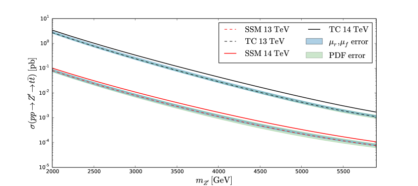
Figure 7: Total cross sections for $pp\to Z^{\prime}\to t\bar{t}$ at the LHC with $\sqrt{S}=13$ TeV (dashed lines) and 14 TeV (full lines) as a function of the $Z^{\prime}$ mass in NLO QCD for the sequential SM (SSM, red) and leptophobic topcolor model (TC, black). For $\sqrt{S}=13$ TeV, we also show the associated scale (blue) and PDF uncertainties (green) (color online).

center-of-mass energy of $\sqrt{S}=13$ TeV in the SSM (dashed red curve) and TC (dashed black curve), together with the associated renormalization and factorization scale uncertainties (blue bands) and PDF uncertainties (green bands). As one can see, in the case of the SSM (lower curves) the PDF uncertainty is larger than the scale uncertainty in the entire range of $m_{Z^{\prime}}$ masses from 2 to 6 TeV considered here. Conversely, for the TC model (upper curves), it is the scale uncertainty which dominates for $m_{Z^{\prime}}\lesssim 5$ TeV, while the PDF uncertainty takes over only at larger values of $m_{Z^{\prime}}$, since the PDFs at large momentum fractions $x_{a,b}$ are less precisely known. The uncertainties at NLO (note that the PS don’t affect the total cross sections) are about $\pm 15$% at low masses and increase to $\pm$35% in the SSM and $\pm 20$% in TC at higher masses. For an integrated luminosity of 100 fb^-1, the number of expected events falls from 10⁴ for $m_{Z^{\prime}}=2$ TeV to 10 for $m_{Z^{\prime}}=6$ TeV in the SSM and is about an order of magnitude larger in TC. When the LHC energy is increased to 14 TeV, the corresponding total cross sections (full curves) at high $Z^{\prime}$-boson mass are larger by about 50%, and the mass reach is extended by about 500 GeV, less of course than the increase in the hadronic energy $\sqrt{S}$, of which only a fraction is transferred to the initial partons and the hard scattering.

Even for resonant-only $Z^{\prime}$-boson production, the $K$-factor is not completely mass-independent, as can be seen in Fig. 8. In TC (lower plot), it increases only modestly from 1.3 to 1.45 in the

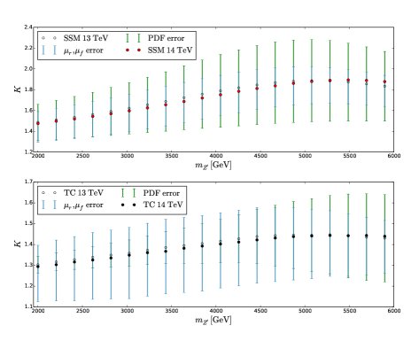
Figure 8: $K$-factors (i.e. ratios of NLO/LO cross sections) at the LHC with $\sqrt{S}=13$ TeV (open circles) and 14 TeV (full circles) as functions of the $Z^{\prime}$ mass for the SSM (top) and TC (bottom). For $\sqrt{S}=13$ TeV, we also show the associated scale (blue) and PDF uncertainties (green) (color online).

mass range considered here, while in the SSM (upper plot) it increases much more from about 1.45 to 1.85. In contrast, it depends very little on the LHC center-of-mass energy of 13 TeV (open circles) or 14 TeV (full circles). In this figure, the scale and PDF uncertainties can also be read off more precisely than in the previous figure.

In Tab. 1 we list the total cross sections in LO for top-pair production at

Table 1: Total cross sections in LO for top-pair production at ${\cal O}(\alpha_{s}^{2})$, ${\cal O}(\alpha_{s}\alpha)$ and ${\cal O}(\alpha^{2})$ in the SM, SSM and TC, together with the corresponding NLO corrections. The $Z^{\prime}$-boson mass is set to 3 TeV.

Order	Processes	Model	$\sigma$ [pb]	$\sigma$ [pb] $(m_{t\bar{t}}>{3\over 4}m_{Z^{\prime}})$
LO	$q\bar{q}/gg\to t\bar{t}$		473.93(7)	0.15202(2)
NLO	$q\bar{q}/gg+qg\to t\bar{t}+q$		1261.0(2)	0.45255(7)
LO	$\gamma g+g\gamma\to t\bar{t}$		4.8701(8)	0.0049727(6)
LO	$\gamma g+g\gamma\to t\bar{t}$ (NLO $\alpha_{s}$ and PDFs)		5.1891(8)	0.004661(6)
LO	$q\bar{q}\to\gamma/Z\to t\bar{t}$	SM	0.36620(7)	0.00017135(3)
NLO	$q\bar{q}\to\gamma/Z\to t\bar{t}$	SM	0.5794(1)	0.00017174(5)
NLO	$q\bar{q}+qg\to\gamma/Z+q\to t\bar{t}+q$	SM	4.176(2)	0.001250(6)
LO	$q\bar{q}\to Z^{\prime}\to t\bar{t}$	SSM	0.0050385(8)	0.0044848(7)
LO	$q\bar{q}\to\gamma/Z/Z^{\prime}\to t\bar{t}$	SSM	0.35892(7)	0.0043464(7)
NLO	$q\bar{q}\to\gamma/Z/Z^{\prime}\to t\bar{t}$	SSM	0.5676(1)	0.005155(3)
NLO	$q\bar{q}+qg\to\gamma/Z/Z^{\prime}+q\to t\bar{t}+q$	SSM	4.172(2)	0.007456(9)
LO	$q\bar{q}\to Z^{\prime}\to t\bar{t}$	TC	0.012175(2)	0.011647(2)
LO	$q\bar{q}\to\gamma/Z/Z^{\prime}\to t\bar{t}$	TC	0.38647(7)	0.011984(2)
NLO	$q\bar{q}\to\gamma/Z/Z^{\prime}\to t\bar{t}$	TC	0.6081(2)	0.01468(1)
NLO	$q\bar{q}+qg\to\gamma/Z/Z^{\prime}+q\to t\bar{t}+q$	TC	4.202(2)	0.01002(1)

${\cal O}(\alpha_{s}^{2})$, ${\cal O}(\alpha_{s}\alpha)$ and ${\cal O}(\alpha^{2})$ in the SM, SSM and TC, i.e. including the SM backgrounds, together with the corresponding NLO corrections. The $Z^{\prime}$-boson mass is set here to 3 TeV, and for our LO predictions we use the NNPDF23_lo_as_0119_qed PDF set, since a set with $\alpha_{s}(m_{Z})=0.118$ is not available at this order. Comparing first the LO results only, we observe that the pure QCD processes of ${\cal O}(\alpha_{s}^{2})$ have a total cross section of about 474 pb, i.e. two orders of magnitude larger than the photon-gluon induced processes of ${\cal O}(\alpha_{s}\alpha)$ with 4.87 pb as naively expected from the ratio of strong and electromagnetic coupling constants in the hard scattering and in the PDFs. The suppression of the pure electroweak with respect to QCD processes is more than three orders of magnitude, as expected from the ratio of coupling constants in the hard scattering and when taking into account that the QCD processes have both quark- and gluon-initiated contributions. The $Z^{\prime}$-mediated processes in the SSM and TC have only cross sections of 5 and 12 fb, respectively compared to 366 fb from the SM channels alone, which therefore clearly dominate the total electroweak cross sections. The interference effects are destructive in the SSM ($-4$%), but constructive in TC ($+2$%).

When a cut on the invariant mass of the top-quark pair of 3/4 of the $Z^{\prime}$ mass (i.e. at 2.25 TeV) is introduced, the SM backgrounds are reduced by more than three orders of magnitude, while the signal cross sections drop only by about 10%. The interference effects then become more important in the SSM ($-7$%), but not in TC ($+2$%) with its very narrow $Z^{\prime}$ width of 1.2% of its mass. While an invariant-mass cut strongly enhances the signal-to-background ratio, the LHC experiments still have to cope with signals that reach only 3 to 8 % of the QCD background, which makes additional cuts on kinetic variables necessary.

The NLO corrections for the QCD processes are well-known and can be computed with the published version of POWHEG (HVQ) Frixione:2007nw . At the LHC with its high gluon luminosity, the $qg$ channels opening up at NLO are known to introduce large $K$-factors, here of about a factor of three. The NLO corrections for the purely electroweak processes are new even in the SM, where we have introduced a proper subtraction procedure for the photon-induced processes. The $K$-factors for the $q\bar{q}$ channel are moderate in the SM (+56%), SSM (+58%) and TC (+56%), where the last two numbers are dominated by SM contributions and therefore very similar. Only after the invariant-mass cut the differences in the models become more apparent in the $K$-factors for the SM ($\pm 0$%), SSM ($+19$%) and TC ($+23$%). However, similarly to the QCD case the $qg$ channel, and also the $\gamma g$ channel opening up for the first time at this order, introduce contributions much larger than the underlying Drell-Yan type Born process. Note that the LO $\gamma g$ cross section computed with NLO $\alpha_{s}$ and PDFs must still be added to the full NLO $q\bar{q}+gg$ cross sections. An invariant-mass cut is then very instrumental to bring down the $K$-factors and enhance perturbative stability, as one can see from the LO $\gamma g$ and in particular the NLO results in the SSM and TC.

4.2 Differential distributions

We now turn to differential cross sections for the electroweak production of top-quark pairs that includes the contribution of a SSM or TC $Z^{\prime}$ boson with a fixed mass of 3 TeV.

The invariant-mass distributions of top-quark pairs in Fig. 9 exhibit steeply falling spectra from the SM background from 10^-2 to 10^-7 pb/GeV together with clearly visible resonance peaks of SSM (top) and TC (bottom) $Z^{\prime}$ bosons at 3 TeV, whose heights and widths differ of course due to the different couplings to SM particles in these two models. In particular, the TC resonance cross section is about an order of magnitude larger than the one in the SSM in accordance with the total cross section results in the previous subsection (see Fig. 7). What becomes also clear from the lower panels in Fig. 9 (top and bottom) is that the $K$-factors are highly dependent on the invariant-mass region and can reach large factors around the resonance region. This is particularly true for TC (bottom), but also for the SSM, and related to the fact that the position of the resonance peak is shifted towards lower invariant masses from LO to NLO due to additional radiation at this order. As one can see, this effect is already present if parton showers are added to the LO calculation, so that the NLO+PS to LO+PS comparison mostly results in an increased $K$-factor at and above the resonance.

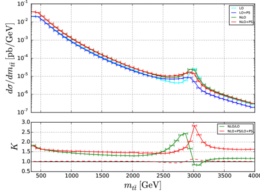
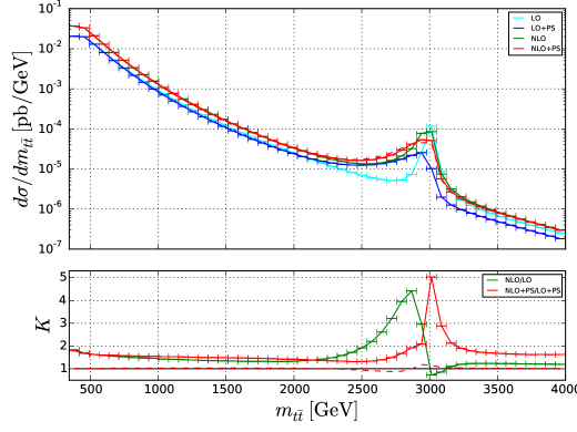
Figure 9: Invariant-mass distributions of top-quark pairs produced through $\gamma$, $Z$ and $Z^{\prime}$ bosons and their interferences at the LHC with $\sqrt{S}=13$ TeV at LO (light blue), LO+PS (dark blue), NLO (green) and NLO+PS (red) accuracy together with the corresponding $K$-factors in the SSM (top) and TC (bottom). The dashed red curves have been obtained with HERWIG 6 Corcella:2000bw instead of PYTHIA 8 Sjostrand:2007gs (color online).

The effect of interferences between SM and new physics contributions is shown in Fig. 10, where the sum of the squared individual contributions (blue) is compared with the square of the sum of all contributions (green) in the SSM (top) and TC (bottom). As one can see, the interference effects shift the resonance peaks to smaller masses, and their sizes are reduced. When the ratios of the two predictions are taken (lower panels), it becomes clear that predictions without interferences overestimate the true signal by a factor of two or more.

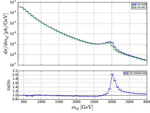
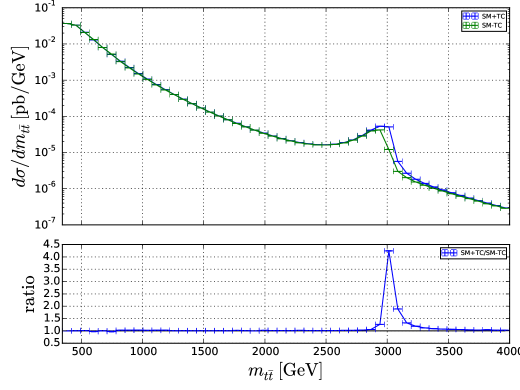
Figure 10: Invariant-mass distributions of top-quark pairs produced through $\gamma$, $Z$ and $Z^{\prime}$ bosons with (green) and without interferences (blue) at the LHC with $\sqrt{S}=13$ TeV at NLO+PS accuracy together with the corresponding ratios in the SSM (top) and TC (bottom) (color online).

The two variables that are particularly sensitive to soft-parton radiation and the associated resummation in NLO+PS Monte Carlo programs are the net transverse momentum of the observed particle (here top-quark) pair ($p_{t\bar{t}}$) and the azimuthal opening angle between them ($\phi_{t\bar{t}}$), which are 0 and $\pi$, respectively, at LO. At NLO they are balanced by just one additional parton and thus diverge and exhibit physical behavior and turnover only at NLO+PS, i.e. after resummation of the left-over kinematical singularities. These well-known facts can also be observed in Figs. 11 and 12, where for obvious reasons the LO $\delta$-distributions at 0 and $\pi$ are not shown. As expected, the NLO (green) predictions diverge close to these end points, while the NLO+PS (red) predictions approach finite asymptotic values. Again, a similar behavior is already observed at LO+PS accuracy, although with different normalization and shape. Interestingly, the resummation works much better for purely $Z^{\prime}$-mediated processes (lower panels) than if SM and interference contributions are included (upper panels). This effect can be traced back to the fact that in the SM-dominated full cross section the top-pair production threshold at $2m_{t}=345$ GeV is almost one order of magnitude smaller than the mass $m_{Z^{\prime}}=3$ TeV governing the exclusive $Z^{\prime}$-boson channel.

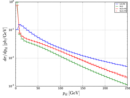
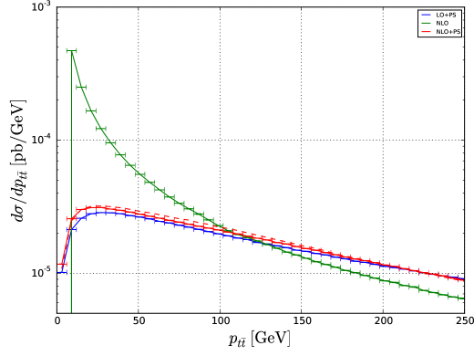
Figure 11: Transverse-momentum distributions of top-quark pairs produced through $\gamma$, $Z$ and $Z^{\prime}$ bosons and their interferences (top) and through $Z^{\prime}$ bosons alone (bottom) at the LHC with $\sqrt{S}=13$ TeV at LO+PS (dark blue), NLO (green) and NLO+PS (red) accuracy in the SSM. The TC distributions look very similar. The dashed red curves have been obtained with HERWIG 6 Corcella:2000bw instead of PYTHIA 8 Sjostrand:2007gs (color online).

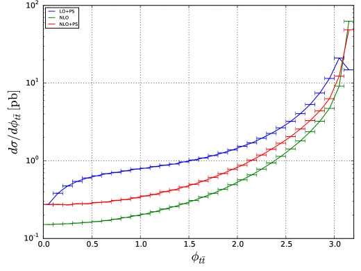
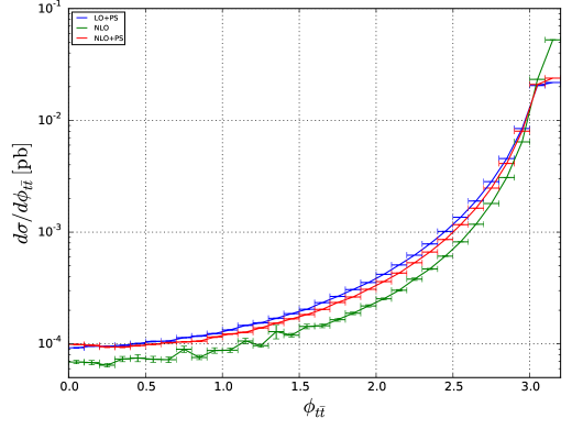
Figure 12: Distributions in the azimuthal opening angle of top-quark pairs produced through $\gamma$, $Z$ and $Z^{\prime}$ bosons and their interferences (top) and through $Z^{\prime}$ bosons alone (bottom) at the LHC with $\sqrt{S}=13$ TeV at LO+PS (dark blue), NLO (green) and NLO+PS (red) accuracy in the SSM. The TC distributions look very similar (color online).

In our discussion of total cross sections in Sec. 4.1, we had included analyses of scale and PDF uncertainties at NLO, but not of the uncertainty coming from different PS implementations, as the PS does not influence total cross sections, but only differential distributions. To estimate this uncertainty, we therefore show in Figs. 9 and 11 also results obtained with the HERWIG 6 PS (dashed red) Corcella:2000bw in addition to those obtained with our standard PYTHIA 8 PS (full red) Sjostrand:2007gs . The dashed red curves in the lower panels of Fig. 9 represent the ratios of the HERWIG 6 over the PYTHIA 8 PS results. As one can see there, the invariant-mass distributions in the SSM and TC are enhanced by the HERWIG 6 PS at the resonance at 3 TeV by about 10%, while the region just below it is depleted by a smaller amount, but over a larger mass region. The PS differences are therefore smaller (by factors of three to six, except for the PDF error in TC) than those of the scale and PDF uncertainties in Fig. 8. The SSM transverse-momentum distribution in Fig. 11 falls off a bit faster with the HERWIG 6 PS than with the PYTHIA 8 PS at large transverse momenta, while in TC it is slightly enhanced at low values, but no significant differences appear between the angularly ordered HERWIG 6 PS and the dipole PS in PYTHIA 8.

The importance of next-to-leading-logarithmic (NLL) contributions that go beyond the leading-logarithmic (LL) PS accuracy can be estimated by a comparison with analytic NLL resummation calculations. These have not been performed for top-quark, but only for lepton final states Fuks:2007gk . In Fig. 5 of this paper, it has been found that the invariant-mass distribution shows no significant difference, while the LL transverse-momentum distribution computed with the HERWIG 6 PS is somewhat smaller than the one obtained with NLL resummation, but that it stays within the residual scale uncertainty of the latter.

Rapidity distributions of the top-quark pair are shown in Figs. 13 and 14. If SM contributions are taken into account (top), they are much flatter than if only the heavy resonance contributes (bottom), i.e. the top-quark pairs are then produced much more centrally. The effect is similar, but somewhat less pronounced in TC (Fig. 14) than in the SSM (Fig. 13) due to the broader resonance in this model. Even for rapidity distributions NLO effects are not simply parametrizable by a global $K$-factor, as it varies from 1.6 to 2.1, when SM contributions are taken into account (blue curves in the upper $K$-factor panels) and drops from 1.6 to 1.4 or even below, if they are not taken into account (blue curves in the lower $K$-factor panels). As expected, the parton showers (green curves in the $K$-factor panels) have little effect on the central parts of the rapidity distributions, and they only slightly influence the forward/backward regions through additional parton radiation from the initial state.

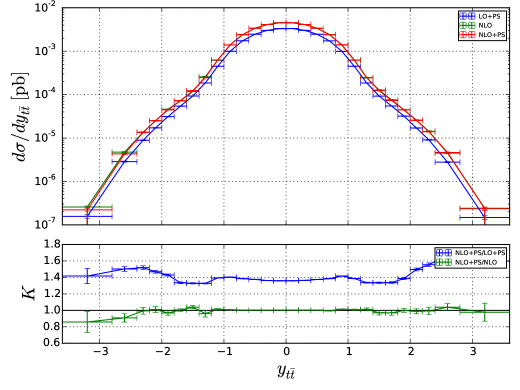
Figure 13: Rapidity distributions of top-quark pairs produced through $\gamma$, $Z$ and $Z^{\prime}$ bosons and their interferences (top) and through $Z^{\prime}$ bosons alone (bottom) at the LHC with $\sqrt{S}=13$ TeV at LO+PS (dark blue), NLO (green) and NLO+PS (red) accuracy together with the corresponding $K$-factors in the SSM. The NLO and NLO+PS curves nearly coincide here (color online).

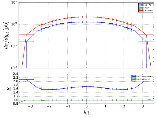
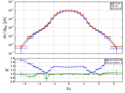
Figure 14: Same as Fig. 13, but for TC (color online).

A particularly sensitive observable for the distinction of new physics models is the forward-backward asymmetry

$$A_{FB} = {N(\Delta y>0)-N(\Delta y<0)\over N(\Delta y>0)+N(\Delta y<0)}$$ (33)

defined at $p\bar{p}$ colliders, where $\Delta y=y_{t}-y_{\bar{t}}$ is the rapidity difference of top and antitop quarks, and the somewhat more complex charge asymmetry

$$A_{C} = {N(\Delta|y|>0)-N(\Delta|y|<0)\over N(\Delta|y|>0)+N(\Delta|y|<0)}$$ (34)

defined at $pp$ colliders, where $\Delta|y|=|y_{t}|-|y_{\bar{t}}|$ is the corresponding difference in absolute rapidity AguilarSaavedra:2012rx . In Fig. 15, the sensitivity of $A_{C}$ to distinguish between the SSM (top) and TC (bottom) is confirmed, as this observable exhibits very different magnitudes at the resonance ($11\pm 1$% vs. $\pm 0.1$%) and far below it ($2.5\pm 0.5$% in both plots), where the SM contributions dominate. Since $A_{C}$ is defined as a ratio of cross sections, NLO and PS corrections cancel to a large extent and are barely visible above the statistical noise. Only for TC, where the rapidity distribution in Fig. 14 (lowest panel) showed distinct features in the ratio of NLO+PS/LO+PS, the transition from the low-mass to the resonance region happens more abruptly in fixed order (NLO) than with PS. If we assume an integrated luminosity of 100 fb^-1 and integrate over an invariant-mass window of 100 GeV around the resonance peak at 3 TeV, one would expect $10^{-5}$ pb/GeV$\times 100$ fb${}^{-1}\times 100$ GeV = 100 events. A 10% asymmetry in the SSM then implies a difference of 10 events with an error of 3, so that $A_{C}=(10\pm 3)\%$. This would be sufficient to distinguish the SSM from the SM and TC.

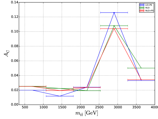
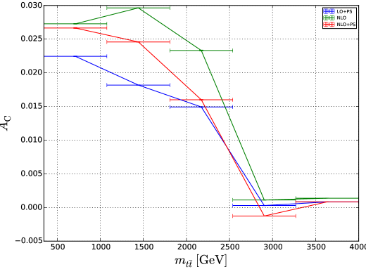
Figure 15: Invariant-mass distributions of the charge asymmetry $A_{C}$ of top-quark pairs produced through $\gamma$, $Z$ and $Z^{\prime}$ bosons and their interferences at the LHC with $\sqrt{S}=13$ TeV at LO+PS (dark blue), NLO (green) and NLO+PS (red) accuracy together with the corresponding $K$-factors in the SSM (top) and TC (bottom) (color online).

5 Conclusions

In this paper we presented the calculation of the ${\mathcal{O}}(\alpha_{S}\alpha^{2})$ corrections to the electroweak production of top-antitop pairs through SM photons, $Z$ and $Z^{\prime}$ bosons, as predicted in the Sequential SM or in tecnicolor models. Our corrections are implemented in the NLO parton shower Monte Carlo program POWHEG. $Z^{\prime}$ reconances are actively searched for by the ATLAS and CMS experiments at the LHC with its now increased center-of-mass energy of 13 TeV. We have consistently included interferences between SM and new physics contributions and have introduced a proper subtraction formalism for QED singularities. With a great variety of numerical predictions, we have demonstrated the mass dependence of the $K$-factor, the changing relative sizes of scale and PDF uncertainties, the large impact of new partonic channels opening up at NLO (in particular of those induced by photon PDFs in the proton), and the non-negligibility of interference effects. Distributions in invariant mass were shown to be particularly sensitive to the latter. The all-order resummation of perturbative corrections implicit in the parton shower has been shown to make the transverse-momentum and azimuthal angle distributions of the top-antitop pair finite and physical. Heavy new gauge-boson contributions were seen to lead to much more centrally produced top pairs, and the charge asymmetry has been shown to be a promising observable to distinguish between different new physics models. Our implementation of this new process in POWHEG, called PBZp, is very flexible, as it allows for the simulation of any $Z^{\prime}$-boson model, and should thus prove to be a useful tool for $Z^{\prime}$-boson searches in the top-antitop channel at the LHC, in particular for leptophobic models.

Acknowledgments

We thank J. Gao for making possible detailed numerical comparisons of our NLO $Z^{\prime}$ calculations as well as R.M. Harris and J. Ferrando for help with matching their LO calculations in the topcolor model. T.J. thanks P. Nason and C. Oleari for useful discussions. This work was partially supported by the BMBF Verbundprojekt 05H2015 through grant 05H15PMCCA, the DFG Graduiertenkolleg 2149, the CNRS/IN2P3 Theory-LHC-France initiative, and the EU program FP7/2007-2013 through grant 302997.

Appendix A Master integrals

The three master integrals needed for the calculation of our NLO corrections are the massive tadpole, $T(m^{2})$, the massless two-point function, $B(0,0,p^{2})$ and the massive two-point function, $B(a,a,p^{2})$. Their analytic expressions in Laurent series of $(D-4)$, up to $\mathcal{O}((D-4))$, are given in the Euclidean region by the following formulas:

$$T(m^{2}) = \mu_{0}^{(4-D)}\int d^{D}k\frac{1}{(k^{2}+m^{2})}\,,$$ (35)

$$= \pi^{\frac{D}{2}}\Gamma\left(3-\frac{D}{2}\right)\,\left(\frac{m^{2}}{\mu_{0}^{2}}\right)^{\frac{D-4}{2}}\!\!\!\!m^{2}\biggl{\{}\frac{2}{(D-4)}-1-\frac{1}{2}(D-4)$$

$$+\mathcal{O}((D-4)^{2})\biggr{\}}\,,$$

$$B(0,0,p^{2}) = \mu_{0}^{(4-D)}\int d^{D}k\frac{1}{k^{2}(p-k)^{2}}\,,$$ (36)

$$= \pi^{\frac{D}{2}}\Gamma\left(3-\frac{D}{2}\right)\,\left(\frac{m^{2}}{\mu_{0}^{2}}\right)^{\frac{D-4}{2}}\biggl{\{}-\frac{2}{(D-4)}+\bigl{[}2+H(0;x)+2H(1;x)\bigr{]}$$

$$+(D-4)\biggl{[}-2+\frac{1}{4}\zeta(2)-H(0;x)-\frac{1}{2}H(0,0;x)-H(0,1;x)$$

$$\hskip 48.36967pt-2H(1;x)-H(1,0;x)-2H(1,1;x)\biggr{]}+\mathcal{O}((D-4)^{2})\biggr{\}}\,,$$

$$B(m^{2},m^{2},p^{2}) = \mu_{0}^{(4-D)}\int d^{D}k\frac{1}{(k^{2}+m^{2})[(p-k)^{2}+m^{2}]}\,,$$ (37)

$$= \pi^{\frac{D}{2}}\Gamma\left(3-\frac{D}{2}\right)\,\left(\frac{m^{2}}{\mu_{0}^{2}}\right)^{\frac{D-4}{2}}\biggl{\{}-\frac{2}{(D-4)}+\biggl{[}2-H(0;x)+\frac{2}{(1-x)}H(0;x)\biggr{]}$$

$$+(D-4)\biggl{[}-2+\frac{1}{(1-x)}\zeta(2)-\frac{1}{2}\zeta(2)-H(-1,0;x)+\frac{2}{(1-x)}H(-1,0;x)$$

$$\hskip 48.36967pt+H(0;x)-\frac{2}{(1-x)}H(0;x)+\frac{1}{2}H(0,0;x)-\frac{1}{(1-x)}H(0,0;x)\biggr{]}$$

$$+\mathcal{O}((D-4)^{2})\biggr{\}}\,,$$

where $p^{2}=m^{2}(1-x)^{2}/x$, $\zeta$ is the Riemann $\zeta$ function and where the functions $H$ denote the harmonic polylogarithms (HPLs) of variable $x$ Remiddi:1999ew ; Goncharov:1998kja .

Appendix B Integrated dipole counter terms

The integrated dipole counter terms are obtained from the general expression Catani:2002hc

$$\mathbb{I}(\varepsilon,\mu_{r}^{2},{p_{i},m_{i}}) = -\frac{\alpha_{S}}{2\pi}\frac{(4\pi)^{\varepsilon}}{\Gamma(1-\varepsilon)}\frac{1}{\mathbb{T}_{i}^{2}}\mathbb{T}_{i}\cdot\mathbb{T}_{j}\times\left[\mathbb{T}_{i}^{2}\left(\frac{\mu_{r}^{2}}{s_{ij}}\right)^{\varepsilon}V_{j}(m_{i},m_{j},\varepsilon)+\Gamma_{j}(m_{j},\varepsilon)\right]\qquad$$

$$+ i\leftrightarrow j+\mathrm{finite\ terms}\,,$$

where $\mathbb{T}^{l}$ denotes the color matrix associated with parton $l$ ($\mathbb{T}^{l}_{cb}=if_{clb}$ for gluons, $\mathbb{T}^{l}_{ab}=t^{l}_{ab}$ and $\mathbb{T}^{l}_{ab}=-t^{l}_{ba}$ for quarks and anti-quarks), $s_{ij}=2p_{i}\cdot p_{j}$, and

$$V_{j}(0,0,\varepsilon) =\frac{1}{\varepsilon^{2}}\,,\ V_{j}(m_{t},m_{t},\varepsilon) =\frac{1}{\varepsilon}\frac{1}{v_{ji}}\ln{\rho}\,,$$ (39)

$$\Gamma_{j}(0,\varepsilon) =\frac{\gamma_{q}}{\varepsilon}\,,\ \Gamma_{j}(m_{j},\varepsilon) =\frac{C_{F}}{\varepsilon}$$ (40)

with $v_{ji}=\sqrt{1-\frac{p_{j}^{2}p_{i}^{2}}{(p_{i}\cdot p_{j})^{2}}}$, $\rho=\sqrt{\frac{1-v_{ji}}{1+v_{ji}}}$ and $\gamma_{q}=3/2C_{F}$. Using Eqs. (B), (39) and (40), we find

$$\mathbb{I}_{\mathrm{init.}} = \frac{2\alpha_{S}}{2\pi}\frac{(4\pi)^{\varepsilon}}{\Gamma(1-\varepsilon)}\left(\left(\frac{\mu_{r}^{2}}{s}\right)^{\varepsilon}\frac{C_{F}}{\varepsilon^{2}}+\frac{\gamma_{q}}{\varepsilon}\right)+\mathrm{finite\ terms}$$ (41)

$$\mathbb{I}_{\mathrm{final}} = \frac{2\alpha_{S}}{2\pi}\frac{(4\pi)^{\varepsilon}}{\Gamma(1-\varepsilon)}\left(\frac{C_{F}}{\varepsilon}\left(\frac{\mu_{r}^{2}}{s-2m_{t}^{2}}\right)^{\varepsilon}\frac{1+x^{2}}{1-x^{2}}\ln{x}+\frac{C_{F}}{\varepsilon}\right)+\mathrm{finite\ terms}\,,$$ (42)

where again $s=m_{t}^{2}(1+x)^{2}/x$ and where the double poles are seen to originate only from initial-state massless quarks. The IR poles are given by the Born cross section multiplied by a factor ${\bf I}_{\rm init}+{\bf I}_{\rm final}$.

References

- (1) ATLAS Collaboration, G. Aad et. al., Observation of a new particle in the search for the Standard Model Higgs boson with the ATLAS detector at the LHC, Phys.Lett. B716 (2012) 1–29, [1207.7214].
- (2) CMS Collaboration, S. Chatrchyan et. al., Observation of a new boson at a mass of 125 GeV with the CMS experiment at the LHC, Phys.Lett. B716 (2012) 30–61, [1207.7235].
- (3) ATLAS, CMS Collaboration, G. Aad et. al., Combined Measurement of the Higgs Boson Mass in Collisions at and 8 TeV with the ATLAS and CMS Experiments, Phys.Rev.Lett. 114 (2015) 191803, [1503.07589].
- (4) K. Hsieh, K. Schmitz, J.-H. Yu, and C.-P. Yuan, Global Analysis of General SU(2) x SU(2) x U(1) Models with Precision Data, Phys.Rev. D82 (2010) 035011, [1003.3482].
- (5) T. Jezo, M. Klasen, and I. Schienbein, LHC phenomenology of general SU(2)xSU(2)xU(1) models, Phys.Rev. D86 (2012) 035005, [1203.5314].
- (6) T. Jezo, M. Klasen, D. R. Lamprea, F. Lyonnet, and I. Schienbein, NLO+NLL limits on and gauge boson masses in general extensions of the Standard Model, JHEP 1412 (2014) 092, [1410.4692].
- (7) T. Jezo, M. Klasen, D. R. Lamprea, F. Lyonnet, and I. Schienbein, NLO+NLL limits on and gauge boson masses, 2015. 1508.03539.
- (8) T. Jezo, M. Klasen, F. Lyonnet, F. Montanet, I. Schienbein, et. al., Can new heavy gauge bosons be observed in ultra-high energy cosmic neutrino events?, Phys.Rev. D89 (2014), no. 7 077702, [1401.6012].
- (9) P. Langacker, The Physics of Heavy Gauge Bosons, Rev.Mod.Phys. 81 (2009) 1199–1228, [0801.1345].
- (10) Particle Data Group Collaboration, K. Olive et. al., Review of Particle Physics, Chin.Phys. C38 (2014) 090001.
- (11) ATLAS Collaboration, G. Aad et. al., Search for high-mass dilepton resonances in pp collisions at TeV with the ATLAS detector, Phys.Rev. D90 (2014), no. 5 052005, [1405.4123].
- (12) CMS Collaboration, C. Collaboration, Search for Resonances in the Dilepton Mass Distribution in pp Collisions at sqrt(s) = 8 TeV, .
- (13) Y. Gao, T. Ghosh, K. Sinha, and J.-H. Yu, G221 Interpretations of the Diboson and Wh Excesses, 1506.07511.
- (14) ATLAS, CDF, CMS, D0 Collaboration, First combination of Tevatron and LHC measurements of the top-quark mass, 1403.4427.
- (15) C. T. Hill, Topcolor: Top quark condensation in a gauge extension of the standard model, Phys. Lett. B266 (1991) 419–424.
- (16) C. T. Hill, Topcolor assisted technicolor, Phys. Lett. B345 (1995) 483–489, [hep-ph/9411426].
- (17) R. M. Harris, C. T. Hill, and S. J. Parke, Cross-section for topcolor Z-prime(t) decaying to t anti-t: Version 2.6, hep-ph/9911288.
- (18) R. M. Harris and S. Jain, Cross Sections for Leptophobic Topcolor Z’ Decaying to Top-Antitop, Eur. Phys. J. C72 (2012) 2072, [1112.4928].
- (19) P. Nason, S. Dawson, and R. K. Ellis, The Total Cross-Section for the Production of Heavy Quarks in Hadronic Collisions, Nucl.Phys. B303 (1988) 607.
- (20) P. Nason, S. Dawson, and R. K. Ellis, The One Particle Inclusive Differential Cross-Section for Heavy Quark Production in Hadronic Collisions, Nucl.Phys. B327 (1989) 49–92.
- (21) W. Beenakker, H. Kuijf, W. van Neerven, and J. Smith, QCD Corrections to Heavy Quark Production in p anti-p Collisions, Phys.Rev. D40 (1989) 54–82.
- (22) W. Beenakker, W. van Neerven, R. Meng, G. Schuler, and J. Smith, QCD corrections to heavy quark production in hadron hadron collisions, Nucl.Phys. B351 (1991) 507–560.
- (23) M. L. Mangano, P. Nason, and G. Ridolfi, Heavy quark correlations in hadron collisions at next-to-leading order, Nucl.Phys. B373 (1992) 295–345.
- (24) W. Bernreuther, A. Brandenburg, Z. Si, and P. Uwer, Top quark spin correlations at hadron colliders: Predictions at next-to-leading order QCD, Phys.Rev.Lett. 87 (2001) 242002, [hep-ph/0107086].
- (25) W. Bernreuther, A. Brandenburg, Z. Si, and P. Uwer, Top quark pair production and decay at hadron colliders, Nucl.Phys. B690 (2004) 81–137, [hep-ph/0403035].
- (26) W. Beenakker, A. Denner, W. Hollik, R. Mertig, T. Sack, et. al., Electroweak one loop contributions to top pair production in hadron colliders, Nucl.Phys. B411 (1994) 343–380.
- (27) C. Kao and D. Wackeroth, Parity violating asymmetries in top pair production at hadron colliders, Phys.Rev. D61 (2000) 055009, [hep-ph/9902202].
- (28) J. H. Kuhn, A. Scharf, and P. Uwer, Electroweak corrections to top-quark pair production in quark-antiquark annihilation, Eur.Phys.J. C45 (2006) 139–150, [hep-ph/0508092].
- (29) S. Moretti, M. Nolten, and D. Ross, Weak corrections to gluon-induced top-antitop hadro-production, Phys.Lett. B639 (2006) 513–519, [hep-ph/0603083].
- (30) W. Bernreuther, M. Fuecker, and Z. Si, Mixed QCD and weak corrections to top quark pair production at hadron colliders, Phys.Lett. B633 (2006) 54–60, [hep-ph/0508091].
- (31) W. Bernreuther, M. Fuecker, and Z.-G. Si, Weak interaction corrections to hadronic top quark pair production, Phys. Rev. D74 (2006) 113005, [hep-ph/0610334].
- (32) W. Hollik and M. Kollar, NLO QED contributions to top-pair production at hadron collider, Phys. Rev. D77 (2008) 014008, [0708.1697].
- (33) J. Gao, C. S. Li, B. H. Li, C.-P. Yuan, and H. X. Zhu, Next-to-leading order QCD corrections to the heavy resonance production and decay into top quark pair at the LHC, Phys.Rev. D82 (2010) 014020, [1004.0876].
- (34) F. Caola, K. Melnikov, and M. Schulze, Complete next-to-leading order QCD description of resonant production and decay into final states, Phys.Rev. D87 (2013), no. 3 034015, [1211.6387].
- (35) S. Frixione and B. R. Webber, Matching NLO QCD computations and parton shower simulations, JHEP 06 (2002) 029, [hep-ph/0204244].
- (36) S. Frixione, P. Nason, and C. Oleari, Matching NLO QCD computations with Parton Shower simulations: the POWHEG method, JHEP 11 (2007) 070, [0709.2092].
- (37) S. Alioli, P. Nason, C. Oleari, and E. Re, A general framework for implementing NLO calculations in shower Monte Carlo programs: the POWHEG BOX, JHEP 06 (2010) 043, [1002.2581].
- (38) B. Fuks, M. Klasen, F. Ledroit, Q. Li, and J. Morel, Precision predictions for - production at the CERN LHC: QCD matrix elements, parton showers, and joint resummation, Nucl. Phys. B797 (2008) 322–339, [0711.0749].
- (39) M. Klasen, C. Klein-Boesing, K. Kovarik, G. Kramer, M. Topp, and J. Wessels, NLO Monte Carlo predictions for heavy-quark production at the LHC: pp collisions in ALICE, JHEP 08 (2014) 109, [1405.3083].
- (40) C. Weydert, S. Frixione, M. Herquet, M. Klasen, E. Laenen, T. Plehn, G. Stavenga, and C. D. White, Charged Higgs boson production in association with a top quark in MC@NLO, Eur. Phys. J. C67 (2010) 617–636, [0912.3430].
- (41) M. Klasen, K. Kovarik, P. Nason, and C. Weydert, Associated production of charged Higgs bosons and top quarks with POWHEG, Eur. Phys. J. C72 (2012) 2088, [1203.1341].
- (42) J. Alwall, R. Frederix, S. Frixione, V. Hirschi, F. Maltoni, O. Mattelaer, H.-S. Shao, T. Stelzer, P. Torrielli, and M. Zaro, The automated computation of tree-level and next-to-leading order differential cross sections, and their matching to parton shower simulations, JHEP 07 (2014) 079, [1405.0301].
- (43) G. Cullen, N. Greiner, G. Heinrich, G. Luisoni, P. Mastrolia, G. Ossola, T. Reiter, and F. Tramontano, Automated One-Loop Calculations with GoSam, Eur. Phys. J. C72 (2012) 1889, [1111.2034].
- (44) CDF Collaboration, T. Aaltonen et. al., Search for Resonant Top-Antitop Production in the Lepton Plus Jets Decay Mode Using the Full CDF Data Set, Phys. Rev. Lett. 110 (2013), no. 12 121802, [1211.5363].
- (45) D0 Collaboration, V. M. Abazov et. al., Search for a Narrow Resonance in Collisions at TeV, Phys. Rev. D85 (2012) 051101, [1111.1271].
- (46) ATLAS Collaboration, G. Aad et. al., A search for resonances using lepton-plus-jets events in proton-proton collisions at TeV with the ATLAS detector, 1505.07018.
- (47) CMS Collaboration, V. Khachatryan et. al., Search for resonant ttbar production in proton-proton collisions at sqrt(s)=8 TeV, 1506.03062.
- (48) J. F. Kamenik, J. Shu, and J. Zupan, Review of New Physics Effects in t-tbar Production, Eur. Phys. J. C72 (2012) 2102, [1107.5257].
- (49) CDF Collaboration, T. Aaltonen et. al., Evidence for a Mass Dependent Forward-Backward Asymmetry in Top Quark Pair Production, Phys. Rev. D83 (2011) 112003, [1101.0034].
- (50) D0 Collaboration, V. M. Abazov et. al., Forward-backward asymmetry in top quark-antiquark production, Phys. Rev. D84 (2011) 112005, [1107.4995].
- (51) M. R. Buckley, D. Hooper, J. Kopp, and E. Neil, Light Z’ Bosons at the Tevatron, Phys. Rev. D83 (2011) 115013, [1103.6035].
- (52) M. Czakon, P. Fiedler, and A. Mitov, Resolving the Tevatron Top Quark Forward-Backward Asymmetry Puzzle: Fully Differential Next-to-Next-to-Leading-Order Calculation, Phys. Rev. Lett. 115 (2015), no. 5 052001, [1411.3007].
- (53) CDF Collaboration, T. Aaltonen et. al., Measurement of the top quark forward-backward production asymmetry and its dependence on event kinematic properties, Phys. Rev. D87 (2013), no. 9 092002, [1211.1003].
- (54) D0 Collaboration, V. M. Abazov et. al., Measurement of the forward-backward asymmetry in top quark-antiquark production in ppbar collisions using the lepton+jets channel, Phys. Rev. D90 (2014), no. 7 072011, [1405.0421].
- (55) J. A. Aguilar-Saavedra, W. Bernreuther, and Z. G. Si, Collider-independent top quark forward-backward asymmetries: standard model predictions, Phys. Rev. D86 (2012) 115020, [1209.6352].
- (56) P. Nogueira, Automatic Feynman graph generation, J.Comput.Phys. 105 (1993) 279–289.
- (57) M. Tentyukov and J. Fleischer, A Feynman diagram analyzer DIANA, Comput.Phys.Commun. 132 (2000) 124–141, [hep-ph/9904258].
- (58) J. Vermaseren, New features of FORM, math-ph/0010025. math-ph/0010025.
- (59) S. Larin, The Renormalization of the axial anomaly in dimensional regularization, Phys.Lett. B303 (1993) 113–118, [hep-ph/9302240].
- (60) M. Veltman, Diagrammatica: The Path to Feynman rules, Cambridge Lect.Notes Phys. 4 (1994) 1–284.
- (61) F. Tkachov, A Theorem on Analytical Calculability of Four Loop Renormalization Group Functions, Phys.Lett. B100 (1981) 65–68.
- (62) K. Chetyrkin and F. Tkachov, Integration by Parts: The Algorithm to Calculate beta Functions in 4 Loops, Nucl.Phys. B192 (1981) 159–204.
- (63) S. Laporta, High precision calculation of multiloop Feynman integrals by difference equations, Int.J.Mod.Phys. A15 (2000) 5087–5159, [hep-ph/0102033].
- (64) C. Studerus, Reduze - Feynman integral reduction in C++, Computer Physics Communications 181 (July, 2010) 1293–1300, [0912.2546].
- (65) A. von Manteuffel and C. Studerus, Reduze 2 - Distributed Feynman Integral Reduction, 1201.4330. arXiv:1201.4330.
- (66) G. ’t Hooft and M. Veltman, Scalar One Loop Integrals, Nucl.Phys. B153 (1979) 365–401.
- (67) S. Catani, S. Dittmaier, M. H. Seymour, and Z. Trocsanyi, The Dipole formalism for next-to-leading order QCD calculations with massive partons, Nucl. Phys. B627 (2002) 189–265, [hep-ph/0201036].
- (68) S. Frixione, Z. Kunszt, and A. Signer, Three jet cross-sections to next-to-leading order, Nucl. Phys. B467 (1996) 399–442, [hep-ph/9512328].
- (69) T. Sjostrand, S. Mrenna, and P. Z. Skands, A Brief Introduction to PYTHIA 8.1, Comput. Phys. Commun. 178 (2008) 852–867, [0710.3820].
- (70) G. Corcella, I. G. Knowles, G. Marchesini, S. Moretti, K. Odagiri, P. Richardson, M. H. Seymour, and B. R. Webber, HERWIG 6: An Event generator for hadron emission reactions with interfering gluons (including supersymmetric processes), JHEP 01 (2001) 010, [hep-ph/0011363].
- (71) R. Frederix, S. Frixione, F. Maltoni, and T. Stelzer, Automation of next-to-leading order computations in QCD: The FKS subtraction, JHEP 10 (2009) 003, [0908.4272].
- (72) T. Jezo, and gauge bosons in SU(2)SU(2)U(1) models: Collider phenomenology at LO and NLO QCD. PhD thesis, LPSC, Grenoble, 2013.
- (73) F. Lyonnet, New heavy resonances: from the Electroweak to the Planck scale. PhD thesis, LPSC, Grenoble, 2014.
- (74) R. K. Ellis and J. C. Sexton, QCD Radiative Corrections to Parton Parton Scattering, Nucl. Phys. B269 (1986) 445.
- (75) L. Barze, G. Montagna, P. Nason, O. Nicrosini, and F. Piccinini, Implementation of electroweak corrections in the POWHEG BOX: single W production, JHEP 04 (2012) 037, [1202.0465].
- (76) L. Barze, G. Montagna, P. Nason, O. Nicrosini, F. Piccinini, and A. Vicini, Neutral current Drell-Yan with combined QCD and electroweak corrections in the POWHEG BOX, Eur. Phys. J. C73 (2013), no. 6 2474, [1302.4606].
- (77) R. D. Ball et. al., Parton distributions with LHC data, Nucl. Phys. B867 (2013) 244–289, [1207.1303].
- (78) NNPDF Collaboration, R. D. Ball, V. Bertone, S. Carrazza, L. Del Debbio, S. Forte, A. Guffanti, N. P. Hartland, and J. Rojo, Parton distributions with QED corrections, Nucl. Phys. B877 (2013) 290–320, [1308.0598].
- (79) S. Frixione, P. Nason, and G. Ridolfi, A Positive-weight next-to-leading-order Monte Carlo for heavy flavour hadroproduction, JHEP 09 (2007) 126, [0707.3088].
- (80) E. Remiddi and J. A. M. Vermaseren, Harmonic polylogarithms, Int. J. Mod. Phys. A15 (2000) 725–754, [hep-ph/9905237].
- (81) A. B. Goncharov, Multiple polylogarithms, cyclotomy and modular complexes, Math. Res. Lett. 5 (1998) 497–516, [1105.2076].