A hard X-ray view of the soft excess in AGN

An excess of X-ray emission below 1 keV, called soft excess, is detected in a large fraction of Seyfert 1-1.5s. The origin of this feature remains debated, as several models have been suggested to explain it, including warm Comptonization and blurred ionized reflection. In order to constrain the origin of this component, we exploit the different behaviors of these models above 10 keV. Ionized reflection covers a broad energy range, from the soft X-rays to the hard X-rays, while Comptonization drops very quickly in the soft X-rays. We present here the results of a study done on 102 Seyfert 1s (Sy 1.0, 1.2, 1.5 and NLSy1) from the Swift BAT 70-Month Hard X-ray Survey catalog. The joint spectral analysis of Swift/BAT and XMM-Newton data allows a hard X-ray view of the soft excess that is present in about 80% of the objects of our sample. We discuss how the soft-excess strength is linked to the reflection at high energy, to the photon index of the primary continuum and to the Eddington ratio. In particular, we find a positive dependence of the soft excess intensity on the Eddington ratio. We compare our results to simulations of blurred ionized-reflection models and show that they are in contradiction. By stacking both XMM-Newton and Swift/BAT spectra per soft-excess strength, we see that the shape of reflection at hard X-rays stays constant when the soft excess varies, showing an absence of link between reflection and soft excess. We conclude that the ionized-reflection model as the origin of the soft excess is disadvantaged in favor of the warm Comptonization model in our sample of Seyfert 1s.

1 Introduction

The typical X-ray spectrum of a Seyfert 1 galaxy is composed of a cut-off power-law continuum, reflection features, low energy absorption, and often an excess in the soft X-ray below 1 keV. The primary continuum power law is believed to stem from Comptonization of optical/UV photons from the accretion disk by energetic electrons in a hot (kT$\sim$100 keV), optically-thin ($\tau\sim 0.5$) corona (Blandford et al. 1990; Zdziarski et al. 1995, 1996; Krolik 1999). The reflection component is composed of a Compton hump peaking at $\sim$ 30 keV and fluorescence lines, the most important of which is the Fe K$\alpha$ line around 6-7 keV. This reflection can be due to reprocessing of the primary X-ray continuum on distant neutral material such as the molecular torus present in the unification model (Antonucci 1993; Jaffe et al. 2004; Meisenheimer et al. 2007; Raban et al. 2009) on the broad- and narrow-line regions (Bianchi et al. 2008; Ponti et al. 2013) or in the accretion disk (George & Fabian 1991; Matt et al. 1991).

While Seyfert 2 galaxies are generally highly absorbed, for example by the dusty torus requested by the unification model (Antonucci 1993), Seyfert 1s are usually not absorbed or only lightly ($N_{\rm\,H}\leq 10^{22}\text{ atoms cm}^{-2}$). When the absorbing material is photoionized, it is referred to as “warm absorber” (George et al. 1998). Absence of absorption allows us to see a soft X-ray emission in excess of the extrapolation of the hard X-ray continuum in many Seyfert 1s below 1 keV. Discovered by Singh et al. (1985) and Arnaud et al. (1985) using HEAO-I and EXOSAT observations, this feature has since then been called soft excess (SE) and is detected in more than 50% of Seyfert 1s (Halpern 1984; Turner & Pounds 1989). This fraction can reach 75% to 90% according to Piconcelli et al. (2005), Bianchi et al. (2009), and Scott et al. (2012). The soft excess was first believed to originate in the inner part of the accretion flow (Arnaud et al. 1985; Pounds et al. 1986), and it has been modeled for a long time using a blackbody with temperatures of $\sim 0.1-0.2$ keV. This model has been ruled out since a standard accretion disk around a supermassive black hole can not lead to such high temperatures (Shakura & Sunyaev 1973). Moreover, the temperature of the blackbody used to model the soft excess has been found to be independent of the black-hole mass, unlike what is expected from a standard accretion disk (Gierliński & Done 2004).

A possible explanation for the soft excess is the “warm” Comptonization scenario: UV seed photons from the disk are upscattered by a Comptonizing corona cooler and optically thicker than the hot corona responsible for the primary X-ray emission. This model has been successfully applied to NGC 5548 (Magdziarz et al. 1998), RE J1034+396 (Middleton et al. 2009), RX J0136.9$-$3510 (Jin et al. 2009), Ark 120 (Matt et al. 2014), and 1H 0419$-$577 (Di Gesu et al. 2014). This Comptonization model is supported by the existence of similarities between the spectral shape (Walter & Fink 1993) and the variability of the optical/UV and soft X-ray emission (Edelson et al. 1996). In a more recent work, Mehdipour et al. (2011) found, in the framework of a multi-wavelength campaign on Mrk 509, a strong correlation between fluxes in the optical/UV and soft X-ray bands, as it would be expected if the soft excess was due to warm Comptonization of the seed photons from the disk. Petrucci et al. (2013) used ten simultaneous XMM-Newton and INTEGRAL observations of Mrk 509 to find that a hot ($kT\sim 100$ keV), optically-thin ($\tau\sim 0.5$) corona is producing the primary continuum and that the soft excess can be modeled well by a warm (kT $\sim$ 1 keV), optically-thick ($\tau\sim$ 10-20) plasma. A warm Comptonization model is also confirmed in Mrk 509 by considering the excess variability in the soft-excess flux on long time scales and variability properties in general (Boissay et al. 2014). Using five observations of Mrk 509 with Suzaku, Noda et al. (2011) showed that the fast variability seen in hard X-rays is not present in the soft X-ray excess. This differential variability rules out a small reflector origin for the soft excess in Mrk 509, similar to what has been shown by Boissay et al. (2014), because the soft X-rays should closely follow the hard X-ray variability in the relativistic ionized reflection models.

Since it is difficult for the Comptonization hypothesis to explain the consistency of the soft-excess feature over a wide range of black-hole masses $M_{\rm\,BH}$, another possible explanation for the soft excess, which is blurred ionized reflection, has been invoked. In this scenario, the emission lines produced in the inner part of the ionized disk are blurred by the proximity of the supermassive black hole (SMBH). Crummy et al. (2006) successfully applied such an ionized-reflection model (reflionx; Ross & Fabian 2005) on a sample of PG quasars to explain the soft excess. Zoghbi et al. (2008) used a similar approach for Mrk 478 and EXO 1346.2+2645. This model has been used to explain the spectral shape, as well as the variability, in MCG$-$6$-$30$-$15 (Vaughan & Fabian 2004) and NGC 4051 (Ponti et al. 2006). Walton et al. (2013) used a sample of 25 bare AGN observed with Suzaku to test the robustness of the reflection interpretation by reproducing the broad-band spectra using the reflionx model (as done by Crummy et al. 2006) and to constrain the black hole spin in many objects of the sample. More advanced blurred ionized-reflection models have been created in recent years, such as relxill, developed by García et al. (2014) and Dauser et al. (2014), which merges the angle-dependent reflection model xillver with a relativistic blurring model relline. This relxill model has already been used to explain the soft excess in Mrk 335 (Parker et al. 2014) and in SWIFT J2127.4+5654 (Marinucci et al. 2014). Vasudevan et al. (2014) showed, using Swift/BAT observations and XMM-Newton/NuSTAR simulations, that a correlation between the reflection and the soft-excess strength is expected if this feature is due to blurred ionized reflection. Parameters obtained when fitting spectra with ionized-reflection models are often extreme. A maximally rotating supermassive black hole and a very steep emissivity are required in most cases (Fabian et al. 2004; Crummy et al. 2006), as well as fine-tuning of the ionization of the disk (Done & Nayakshin 2007). These parameters, which are similar to those obtained when modeling the broad component of the Fe K$\alpha$ line (Fabian et al. 2005), show that in this scenario most of the reprocessed radiation is produced very close to the event horizon. Time delays between iron lines and direct X-ray continuum have been detected in several objects (e.g., 1H 0707$-$495, Fabian et al. 2009; NGC 4151, Zoghbi et al. 2012; MCG$-$5$-$23$-$16 and NGC 7314, Zoghbi et al. 2013; Ark 564 and Mrk 335, Kara et al. 2013). Soft X-ray reverberation lags have been detected in a considerable sample of objects (Cackett et al. 2013; de Marco et al. 2011; De Marco et al. 2013) and are interpreted as a signature of reverberation from the disk, which would support the reflection origin for the soft excess. However, if soft lags are detected on short time scales, the soft X-ray emission can lead the hard band on long time scales, as in PG 1244+026 (Gardner & Done 2014). In this case, the soft excess is interpreted as a combination of intrinsic fluctuations propagating down through the accretion flow giving the soft lead and reflection of the hard X-ray emission giving the soft lag.

Using a sample of six bare Seyfert galaxies, Patrick et al. (2011) modeled the Suzaku broad-band spectra with both ionized reflection and additional Compton scattering components. Combining the two models to reproduce the soft excess provided better fitting results with lower values of the spin and emissivity index. Other works presenting direct tests of the ionized reflection versus warm Comptonization include, for example, analyses from Lohfink et al. (2013) and Noda et al. (2013). Lohfink et al. (2013) used archival XMM-Newton and Suzaku observations of Mrk 841 to test different models for the origin of the soft excess in a multi-epoch fitting procedure. Noda et al. (2013) fit Suzaku spectra of five AGN with different models to reproduce the soft excess and concluded that the thermal Comptonization model reproduces the data better.

The soft excess could also be the signature of strong, relativistically smeared, partially ionized absorption in a wind from the inner disk, as proposed for PG 1211+143 by Gierliński & Done (2004). In the case of a totally covering absorber, extreme parameters are needed to reproduce the observed soft excess, as in the case of blurred ionized-reflection models. For example, a very high smearing velocity ($v\sim 0.3c$) is required, but such a velocity is difficult to reach considering radiatively driven accretion disk winds (Schurch & Done 2007; Schurch et al. 2009). We do not further discuss this model in this paper.

This papers aims to test blurred ionized-reflection models as the origin of the soft excess, in particular in the lamp-post configuration, via a spectral model-independent analysis. Different scenarii of the origin of the soft excess imply different behaviors in the soft and hard X-ray bands, since ionized reflection covers a broad energy range, while Comptonization drops very quickly in the soft X-rays. Because we want to get good constraints on the hard X-ray reflection measurements, we consider sources detected by the Swift/BAT instrument and combine these observations with data from the XMM-Newton satellite to get information about the soft excess. We carry out broad-band (0.5-100 keV) spectral analysis of the sources and explore the relations between the parameters resulting from the fitting procedure. We compare the reflection and soft-excess parameters with those obtained from simulations in a lamp-post configuration. We also study the differences between soft and hard X-ray emission by stacking the XMM-Newton and BAT spectra according to their soft-excess strengths.

2 Sample and data analysis

We use a sample of sources from the Swift (Gehrels et al. 2004) BAT 70-Month Hard X-ray Survey catalog (Baumgartner et al. 2013), which contains 1210 sources including 292 Seyfert 1s. By cross-correlating the Swift/BAT catalog with the Veron catalog (Véron-Cetty & Véron 2010), we selected only narrow-line Seyfert 1s (NLSy1s) and Seyfert 1s - 1.5s (Sy1s - 1.5s). Our sample is in this way composed of 102 sources, divided in 37 Sy1.0s, 18 Sy1.2s, 35 Sy1.5s, and 12 NLSy1s. We selected sources that have been observed with the XMM-Newton satellite (Jansen et al. 2001) as pointed observations with a minimum exposure time of 5 ks (see Table LABEL:tab:epic_info). We selected sources with a flux higher than $10^{-11}\text{ergs}/\text{s}/\text{cm}^{2}$ in the 14-195 keV band. BAT spectra (Barthelmy et al. 2005) have been obtained from the Swift/BAT website .

To study the soft X-ray emission of these objects, we used XMM-Newton observations. In the case of multiple observations for the same source, we considered the observation with the longest exposure time (see Table LABEL:tab:epic_info). Data was reduced on the original data files using the XMM-Newton Standard Analysis Software (SAS v12.0.1 - Gabriel et al. 2004) considering both the PN (Strüder et al. 2001) and MOS (Turner et al. 2001) spectra of each source. Events were filtered using #XMMEA_EP and #XMMEA_EM, for PN and MOS cameras, respectively. Single and double events were selected for extracting PN spectra and single, double, triple, and quadruple events were considered for MOS. The data were screened for any increased flux of background particles. Spectra were extracted from a circular region of 30 arcsec centered on the source. The background was extracted from a nearby source-free region of 40 arcsec in the same CCD as the source. The XMM-Newton data showed evidence of significant pile-up in some objects (see Table LABEL:tab:epic_info), for which the extraction region used was an annulus of inner radius 15 arcsec instead of a simple circle. Response matrices were generated for each source spectrum using the SAS arfgen and rmfgen tasks.

3 Spectral analysis

In this section, we explain the broad-band spectral analysis procedure of all the sources of our sample between 0.5 and 100 keV. More precisely, we fit the 3-100 keV data with a phenomenological model and then quantify the soft excess below 2 keV with respect to this model. We present different fitting models, taking reprocessing into account that is mainly due to distant and/or local reflectors.

3.1 Spectral fitting procedure

3.1.1 Reprocessing mainly due to a distant reflector

The spectral analysis of our sample is performed using the general X-ray spectral-fitting program XSPEC (version 12.8.1, Arnaud 1996). To determine specific parameters for each object of our sample, we analyzed PN and MOS spectra from the XMM-Newton satellite and BAT spectra from Swift.

We first chose to fit PN/MOS and BAT spectra jointly in an energy band in which there is little contamination from the soft excess or absorption (from 3 to 100 keV) with a cut-off power law and a neutral reflection component using the pexmon model (Nandra et al. 2007) from XSPEC. The pexmon model is similar to the pexrav model (Magdziarz & Zdziarski 1995), but includes Fe K$\alpha$, Fe K$\beta$, and Ni K$\alpha$ lines and the Fe K$\alpha$ Compton shoulder (George & Fabian 1991). We use the pexmon model to take the reflection component into account, the cut-off power-law component being modeled by cutoffpl. We also take Galactic absorption (abs${}_{\texttt{Gal}}$) into account, fixing the value of $N_{\rm\,H}^{G}$ to the one found in the literature (Dickey & Lockman 1990) (see Table LABEL:tab:epic_info).

The pexmon model includes the narrow iron lines produced by reflection from distant neutral material, such as the broad-line region (e.g., Bianchi et al. 2008), the molecular torus (e.g., Shu et al. 2011; Ricci et al. 2014), or the region between the torus and the broad-line region (Gandhi et al. 2015). However, assuming that the primary X-ray continuum is also reprocessed in the innermost part of the accretion disk, these iron lines should be broadened by Doppler motion and relativistic effects (e.g., Fabian et al. 1989). To consider these effects, we allow broadening of the iron line from pexmon, by convolving the pexmon model with a Gaussian smoothing model gsmooth ($\sigma$ can vary between 0.0 and 0.5 keV).

XMM-Newton and Swift/BAT observations are not simultaneous because BAT spectra are integrated over 70 months, so variability in flux can occur between XMM-Newton and Swift/BAT spectra. To correct the flux variability during the fitting procedure, we multiply the cut-off power-law of our model by a cross-calibration factor $f$. The pexmon component parameters are fixed to the same value for XMM-Newton and BAT. When doing so, we consider that the reflection component, assumed to be mainly due to a distant reflector, does not vary on the BAT time scale and that only the primary continuum does. The cross-calibration factor $f$ is fixed to 1 for BAT spectra and left free between 0.7 and 1.3 for XMM-Newton spectra ($f$ is found to be consistent with being equal for PN and MOS spectra). Using this $f$ factor, we constrain the fit sufficiently while taking the flux variability of the primary continuum between XMM-Newton and BAT into account.

The resulting model for the fit between 3 and 100 keV is

abs${}_{\texttt{Gal}}$ (f$\times$cutoffpl+gsmooth*pexmon).

When fitting the XMM-Newton and Swift/BAT spectra between 3 and 100 keV, we keep the inclination angle of the disk to its default value of 60^∘. Abundances in pexmon are free to vary between 0.3 and 3 (relative to solar), in order to properly model the iron line as well as the Compton hump. The high-energy cut-off can vary from 100 to 500 keV. The reflection factor $R$, which is the strength of the reflection component relative to what is expected from a slab subtending $2\pi$ solid angle, can have values between 0 and 100. We find the best fit parameter values using the $\chi^{2}$ statistics of XSPEC.

To study the soft X-ray emission of the objects, we fix the parameters of the model described previously to the values found during the fit between 3 and 100 keV and add XMM-Newton data in the 0.5 to 3 keV energy band. We remove the gsmooth component from our model to avoid spurious features at low energy (arising from the convolution at the edge of the spectrum). Suppressing this component will just slightly degrade the $\chi^{2}$ value and give an advantage in computation time.

Since we want this analysis to be model independent, we do not favor any hypothesis here for the origin of the soft excess. To measure the strength of the soft excess, we use a Bremsstrahlung model that provides a good phenomenological representation of its smooth spectral shape. We then find the best-fit parameter values using the $\chi^{2}$ statistics, fitting the spectra between 0.5 and 100 keV. In the majority of the objects of our sample, the soft excess is fit better by two Bremsstrahlung models than by a single one with plasma temperatures between 0 and 1 keV.

We also evaluate the presence of absorption from a cold or ionized medium (abs${}_{\texttt{cold/warm}}$). The presence of a single or double warm absorber (WA), modeled by XSTAR, and/or of a cold absorber, modeled by zwabs, is verified by an F test between the model that takes only the soft excess into account and the one that includes the absorber.

The resulting broad-band-fitting model is

abs${}_{\texttt{Gal}}$$\times$abs${}_{\texttt{cold/warm}}$ (bremss+bremss+f$\times$cutoffpl+pexmon).

3.1.2 Reprocessing mainly due to a local reflector

In Sect. 3.1.1, we considered that the reflection component is mainly due to a distant reflector, which is expressed by the cross-calibration being applied to the power law and not to the pexmon component in the fitting procedure. We also want to study the case where the reflection is mainly due to a local reflector. The model used for this hypothesis to fit the 3 to 100 keV band is

abs${}_{\texttt{Gal}}$$\times$f (cutoffpl+gsmooth*pexmon).

Applying this $f$ cross-calibration factor on the pexmon component this time allows us to consider that the reflection responds with very little lag to the continuum. We fit this new model on our objects with the same ranges of parameters as described in Sect. 3.1.1. The fitting procedure between 0.5 and 100 keV is the same as the one described in Sect. 3.1.1 with the model

abs${}_{\texttt{Gal}}$$\times$abs${}_{\texttt{cold/warm}}$ (bremss+bremss+f (cutoffpl+pexmon)).

3.1.3 Comparison between local and distant reflection models

For each object of our sample, we perform a statistical F test between models of local and distant reflection. We can see in Fig. 1 that, considering the theoretical F values range from the Fisher table for which we can accept the null hypothesis at a 95% significance level (see red area in Fig. 1), only 8% of our objects are better fit by the local reflection model and 3% by the distant reflection model. The average value of F being less than 1 ($\text{F}_{\text{mean}}$=0.98) shows a little preference for the local-reflection model to fit our data, but since $\text{F}_{\text{mean}}$ is inside the acceptance zone, this preference is not significant. We therefore cannot distinguish between the local-reflection and the distant-reflection models here.

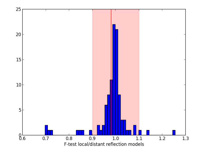
Figure 1: Distribution of the F test results between the local reflection model and the distant reflection model used to fit each object. The red area is the acceptance zone of the null hypothesis. The average F value, represented by the red line, is inside the acceptance zone.

The X-ray spectra of our Seyfert galaxies should present iron emission lines with two components: the narrow line coming from reflection on the dusty torus or the broad-line region and on the broad line thought to be produced in the inner accretion disk. The total reflection factor includes the reflection strengths of both components. In the hypothesis where the soft excess is due to ionized reflection, the broad line is expected to be more important than the narrow one, which is why we use a gsmooth model to allow the broadening of the iron line from the pexmon model. Furthermore, we have just seen that changing the input of the cross-calibration factor to account for local and distant reflections does not allow us to distinguish the models. However, to check that we do not miss any information from the narrow iron lines, we tested a fitting procedure with two pexmon models on 10% of the objects of our sample. One simple pexmon model was used to reproduce the narrow iron line, and the second one, convolved with a gsmooth model, represents the broad component. The sum of the reflection fractions from the two pexmon models is equal to the reflection fraction measured with our one-pexmon fitting procedure. This test was done on ten objects for which we have good signal-to-noise data. As the results are consistent between the two approaches and as the reflection factor is better constrained in our initial fitting procedure, we chose to keep this one-reflection fitting process to model our data.

3.2 Soft excess and absorption properties

The results obtained by our spectral analysis, which is based on the hypothesis of a reflection due mainly to distant material, are presented in Table LABEL:tab:fit. We find that 79 objects (i.e., 80% of our sample) present a soft excess (SE). Among these 79 objects showing a soft excess, 42 do not show the presence of absorption and 37 are hardly absorbed by cold or warm material.

The 24 other objects show the presence of a stronger absorption by a cold or warm absorber with a column density value $N_{\rm\,H}\geq 10^{22}\text{ atoms cm}^{-2}$. These absorbers prevent a good measurement of an eventual soft excess. Twelve of these strongly absorbed objects present a complex absorption and are labeled in Table LABEL:tab:fit:

1. ESO 323$-$77: Miniutti et al. (2014) used multi-epoch spectra from 2006 to 2013 to show that the absorption is due to a clumpy torus, broad-line regions, and two warm absorbers.

2. EXO 055620$-$3820.2: Turner et al. (1996) found by using ASCA observations that the continuum of the source is attenuated by an ionized absorber either fully or partially covering the X-ray source.

3. IC 4329A: Steenbrugge et al. (2005) used XMM-Newton observations to show that the absorber is composed of seven different absorbing systems.

4. MCG$-$6$-$30$-$15: Miyakawa et al. (2012) fit Suzaku data considering absorbers with only a variable covering factor.

5. Mrk 1040: Reynolds et al. (1995) found that the soft spectral complexity visible in ASCA observations could be either explained by a soft excess and by intrinsic absorption or by a complex absorber.

6. Mrk 6: Mingo et al. (2011) showed that the variable absorption visible in XMM-Newton and Chandra observations are probably caused by a clump of gas close to the central AGN in our line of sight.

7. NGC 3227: Beuchert et al. (2014) used Suzaku and Swift observations of a 2008 eclipse event to characterize the variable-density absorption, probably caused by a filamentary, partially covering, and moderately ionized cloud.

8. NGC 3516: Huerta et al. (2014) showed that this object is absorbed by four warm absorbers according to nine XMM-Newton and Chandra observations.

9. NGC 3783: Brenneman et al. (2011) used Suzaku observations to show the presence of a multicomponent warm absorber.

10. NGC 4051: Pounds & King (2013) used a XMM-Newton observation to find a fast, highly ionized wind, launched from the vicinity of the supermassive black hole, that shocked against the interstellar medium (ISM). They speculate that the warm absorbers often observed in AGN spectra result from an accumulation of such shocked winds.

11. NGC 4151: Wang et al. (2011) found, in a Chandra observation, emission features in soft X-rays that are consistent with blended brighter O VII, O VIII, and Ne IX lines. They also found low and high ionization spectral components that are consistent with warm absorbers.

12. UGC 3142: Ricci et al. (2010) used XMM-Newton, Swift, and INTEGRAL data for the spectral analysis. This object is absorbed by two layers of neutral material.

We decide not to include these 23 absorbed objects in our analysis in order to have a clean measurement of the soft-excess intensity.

3.3 Soft-excess strength

For the following analysis, we keep only the 79 objects that show the presence of soft excess and that are absorbed by a material with a $N_{\rm\,H}$ smaller than $10^{22}\text{ atoms cm}^{-2}$. For each of these objects, we define the strength of the soft excess q as the ratio between the flux of the soft excess (i.e., the flux of the Bremsstrahlung models between 0.5 and 2 keV) and the extrapolated flux of the continuum between 0.5 and 2 keV. This definition differs from the one used in Vasudevan et al. (2014), as discussed in Sect. 4.2.

4 Relation between reflection and soft-excess strength

In this section, we compare the reflection and soft-excess strength from data with those obtained from simulations of blurred ionized reflection. These simulations, similar to the ones of Vasudevan et al. (2014), are performed using the lamp-post configuration of the relxill model of García et al. (2014) and Dauser et al. (2014), changing the height of the source that controls the emissivity index and the reflection fraction and changing the mass accretion rate that controls the inner disk ionization. The resulting simulated spectra are then fit with the same phenomenological model than real data to compare the distributions of soft-excess strength versus reflection strength from the real and simulated data.

4.1 $R$ vs $q$ in the sample

To study the evolution of the soft excess with reflection, we plot, in top panel of Fig. 2, the reflection factor measured when fitting XMM-Newton (EPIC PN and MOS) and Swift/BAT spectra as a function of the soft-excess strength $q$. In the case of distant reflection (see Sect. 3.1.1), we find an anti-correlation characterized by a Spearman coefficient of r=-0.33 and a null-hypothesis probability of about 0.3%. We perform a bootstrap on the data, finding a 99.9% confidence interval (CI) for the Spearman correlation coefficient of $-0.62\leq r\leq 0.01$ and a probability of having a negative correlation of 99.8%.

Our sample includes NLSy1s, objects that often present a strong soft excess and a steep spectrum (e.g., Vaughan et al. 1999; Haba et al. 2008; Done et al. 2013). If we do not include the ten NLSy1s in our analysis, we still find a correlation with a Spearman coefficient of $r=-0.31$, a null-hypothesis probability of about 0.7% and a probability of 99% of having a negative correlation between $R$ and $q$.

To look at the effect of the warm absorber in the objects of our sample, we only consider the 42 objects showing a soft excess without absorber. Spearman statistics give a correlation coefficient of r=-0.37 with a null-hypothesis probability of 2% and the probability of having a negative correlation of 98%. The anti-correlation between $R$ and $q$ found with the entire sample of objects showing a soft excess with or without absorber still exists when considering only objects without absorber. In this case, the anti-correlation is less significant because it is based on about half of the sample.

To consider errors in both x and y axes, as well as intrinsic scatter, we performed a linear regression with a Bayesian approach using an IDL procedure called linmix_err (Kelly 2007). The linear regression process results in the relation:

$$R=-0.72\,_{-0.21}^{+0.28}\times q+1.01\,_{-0.11}^{+0.18}.$$ (1)

The intrinsic scatter of $R$ is 0.37. The Markov Chains Monte Carlo (MCMC) created by the IDL procedure allowed us to plot the 99.9% CI for this linear regression (blue contour in top panel of Fig. 2).

Figure 2: Reflection factor $R$ as a function of the strength of the soft excess $q$ (in the case of distant reflection). Top panel: Linear regression performed using the linmix_err procedure is represented by the blue line, and 99.9% CI is given by the blue contour. The red line represents the positive correlation expected if the soft excess is due to ionized reflection (result of relxilllp_ion simulations, see Sect. 4.2). Density contours of the simulations are plotted in red (solid line: 68%; dashed line: 90%). Bottom panel: Blue points represent our 79 objects showing a soft excess. They are mostly contained (75%) in the blue box ($R<2.0$ and $q<0.75$). Red triangles are relxilllp_ion simulation results.

In the case of local reflection (see Sect. 3.1.2), Spearman statistics give a correlation coefficient of r=-0.48 between $R$ and $q$ and a null-hypothesis probability of 0.06%. The linear regression performed with linmix_err results in the relation:

$$R=-0.54\,_{-0.12}^{+0.09}\times q+0.94\,_{-0.01}^{+0.20}.$$ (2)

The intrinsic scatter of $R$ is 0.24.

If we only consider NLSy1 galaxies, Spearman statistics give a correlation coefficient of r=-0.36, a null-hypothesis probability of 31% and a probability of 87% of a negative correlation. The significance of this result is still quite strong considering that our sample contains only ten NLSy1s for which we can measure the soft excess.

4.2 $R$ vs $q$ in simulations of ionized reflection

Vasudevan et al. (2014) performed $\sim$2400 XMM–Newton and NuSTAR simulations of blurred ionized reflection, using reflionx and kdblur and taking neutral reflection with pexrav into account. They used a wide range of values for the iron abundance, the photon index, the ionization, and the ratio between the normalizations of pexrav and reflionx. They fixed the emissivity index and the inclination to intermediate values and fixed the high energy cut-off to $10^{6}$ keV. The strength of the hard excess $R$ was then measured by a neutral reflection model pexrav (the iron line being modeled by a Gaussian component) and the soft excess was modeled by a blackbody. They fixed the normalizations of each component of this model, in order to constrain the blackbody temperature and the Gaussian line energy and width. They defined the soft-excess strength as being the ratio between the luminosity from the blackbody between 0.4 and 3 keV and the power-law luminosity between 1.5 and 6 keV. Their simulations predict the existence of a correlation between $R$ and the soft-excess strength.

We want to determine the expected relation between the reflection factor and the soft-excess strength in the case of ionized reflection, similar to what was done by Vasudevan et al. (2014). But since we want to use a more recent ionized-reflection model and our spectral fitting procedure differs from the one of Vasudevan et al. (2014), we performed simulations using the relxilllp_ion model. The relxilllp_ion model (Dauser et al. 2014) is similar to the relxill model, but adapted for the lamp-post geometry. By simulating this lamp-post configuration, we assumed an explicit link between the smearing and the amount of reflection. For example, for objects, such as 1H 0707$-$495, that have a high emissivity index and are thus strongly smeared, the compact source is thought to be confined to a small region around the rotation axis and close to the black hole (Fabian et al. 2012). The very small height $h$ required predicts a very large reflection fraction $R$ (see the relation between $R$ and $h$ plotted in Figure 2 of Dauser et al. 2014). The ionization of the accretion disk depends on the mass accretion rate $\dot{m}$ and on the density profile of the disk. The density structure assumed in a hydrostatic $\alpha$ disk (Shakura & Sunyaev 1973) is not always appropriate. In particular, it has been shown that the accretion disk cannot be in hydrostatic equilibrium if the soft excess is made via reflection (Done & Nayakshin 2007). In the relxilllp_ion model, the gas in the atmosphere of the accretion disk is assumed to be at a constant density (García et al. 2014).

We simulated Swift/BAT and XMM-Newton/PN spectra with a signal-to-noise ratio comparable to our data (time exposure of 10 ks for XMM-Newton/PN and 1 Ms for Swift/BAT). We performed $\sim$3500 simulations with different values of relxilllp_ion parameters for the reflection factor $R_{rel}$ (from 0 to 100, values that are reachable in a lamp-post configuration for a source very close to the black hole, see Fig. 5 in Miniutti & Fabian 2004), the photon index $\Gamma_{rel}$ (from 1.4 to 2.5), the ionization parameter at the inner edge of the disk ($log(\xi)$ between 0.0 and 4.7, as allowed by the model), the abundances $A_{Fe}$ (from 0.3 to 3.0 in solar unit), the height $h$ of the source (from 1 to 6 $r_{g}$), the inner radius $R_{in}$ (from 1 to 50 $r_{g}$), the density index (from 0 to 4), the mass accretion rate $\dot{m}$ (from 0.01 to 5), and the high-energy cut-off $Ec_{rel}$ (from 100 to 300 keV). To account for the narrow component of the iron line in our simulated spectra, we added a pexmon component to our relxilllp_ion model so as to reproduce the neutral reflection on the dusty torus and broad-line regions, with a reflection factor $R_{narrow}$ varying between 0 and 1. Considering only Seyfert 1s and according to the unification model, we performed simulations for different inclination values $\theta$ between 0^∘ and 60^∘, giving the weight $sin(\theta)$ to each simulation to take the probability of having such an inclination into account.

We fit our simulated relxilllp_ion spectra by using the fitting procedure explained in Sect. 3.1, in order to measure the photon index and the reflection from the pexmon model, as well as the value of the soft-excess strength $q$ and to be able to compare them to the parameters obtained when fitting the real data. We performed a linear regression (red solid line in top panel of Fig. 2) and plotted density contours of the simulated data (red contours in top panel of Fig. 2; solid line: 68%, dashed line: 90%). Similar to Vasudevan et al. (2014), we expected to find a positive correlation between the reflection factor $R$ and the soft-excess strength $q$, if ionized reflection model is the explanation of the soft excess, even if the simulations and the soft-excess strength definition are slightly different. We found such a positive correlation with our simulations, assuming all relxilllp_ion parameters are uncorrelated. Spearman statistics give a correlation coefficient between $R$ and $q$ expected for ionized-reflection model of r=0.55 and a negligible null-hypothesis probability. The expected relation is

$$R=6.17\,_{-0.20}^{+0.19}\times q+2.80\,_{-0.11}^{+0.11}.$$ (3)

The bottom panel of Fig. 2 shows the reflection factor $R$ measured by pexmon as a function of the soft-excess strength $q$ for real and simulated data. Blue points represent the real data, i.e. results of the fitting of the objects of our sample, and red triangles are the parameters obtained by simulating relxilllp_ion models (red contour in top panel of Fig. 2 has been derived from these red triangles). As we can see in bottom panel of Fig. 2, 75% of the blue data points are contained in the blue box ($R<2.0$ and $q<0.75$). Relxilllp_ion simulations result in similar parameters, but also in higher reflection factors and higher soft-excess strengths. Twenty-five percent of our simulated objects are in the blue box, and 75% of them are outside the blue box. We do not observe any high-$R$ objects, unlike what is expected with blurred ionized-reflection models (with the relxilllp_ion model in our simulations, and with the reflionx model in simulations from Vasudevan et al. 2014).

5 Evolution of the photon index of the primary continuum

In this section, we explore the relations between the photon index of the primary continuum and the reflection and soft-excess strength. We compare the parameters derived from data analysis with those obtained from simulations of lamp-post configuration.

5.1 Soft excess and photon index

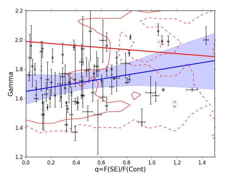
Figure 3: Strength of the soft excess against the power-law slope obtained with XMM-Newton and BAT data (in the case of distant reflection). CI is represented by the blue contour. The red line represents the relation expected in the case of ionized reflection; the red contours are the result of relxilllp_ion simulations (solid line: 68%, dashed line: 90%).

We plot in Fig. 3 the photon index of the primary continuum as a function of the soft-excess strength $q$ (in the case of distant reflection). This plot reveals a hint of a weak correlation between $\Gamma$ and $q$. Indeed, Spearman rank analysis gives a correlation coefficient of r=0.19 and a null-hypothesis probability of about 10%. A bootstrap on the data points gives a probability of 91% of a positive correlation. We use the Bayesian linmix_err procedure to perform a linear regression. We obtain

$$\Gamma=0.14\,_{-0.06}^{+0.05}\times q+1.65\,_{-0.02}^{+0.04}.$$ (4)

The intrinsic scatter of $\Gamma$ is 0.32. CI is the blue contour in Fig. 3.

Removing the NLSy1s from our sample still gives a probability of having a positive correlation of 87%. If we do not consider objects with warm absorber, we have a probability of 85% of a positive correlation.

The possible faint correlation between the photon index of the primary power law and the soft-excess strength is also found in the case of reflection mainly owing to a local reflector with a Spearman correlation coefficient of r=0.14 and a null-hypothesis probability of 21%. We find the relation:

$$\Gamma=0.11\,_{-0.03}^{+0.08}\times q+1.71\,_{-0.06}^{+0.001}.$$ (5)

The intrinsic scatter of $\Gamma$ is 0.30.

If we only consider the ten NLSy1 objects of our sample, Spearman statistics give a correlation coefficient of r=0.50, a null-hypothesis probability of 14%, and a probability of 96% of a positive correlation.

This correlation between the photon index and the soft-excess strength is consistent with the result of Page et al. (2004b), who found a correlation with a $\sim$ 4% null-hypothesis probability obtained with seven objects observed by XMM-Newton.

The red line in Fig. 3 represents the relation between $\Gamma$ and $q$ expected in the case of ionized reflection. Density contours of the relxilllp_ion simulations described in Sect. 4.2 are plotted in red (solid line: 68%; dashed line: 90%). Spearman statistics give a correlation coefficient of r=-0.07 and a null-hypothesis probability of $2\times 10^{-5}$%. The relation is

$$\Gamma=-0.07\,_{-0.01}^{+0.01}\times q+1.99\,_{-0.008}^{+0.008}.$$ (6)

The results of the simulations are inconsistent with our observational results.

5.2 Reflection and photon index

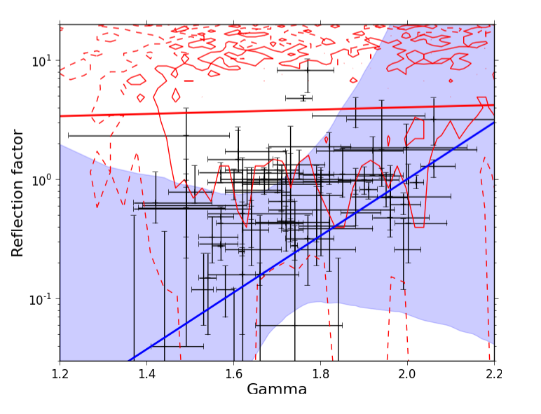
Figure 4: Reflection factor against the power-law slope obtained with XMM-Newton and BAT data (in the case of distant reflection). CI is represented by the blue contour. The red line represents the relation between $R$ and $\Gamma$ in the case of ionized reflection. Density contours are plotted in red (solid line: 68%, dashed line: 90%).

We plot in Fig. 4 the reflection factor as a function of the photon index (in the case of reflection mainly due to a distant reflector). Spearman statistics show that a positive correlation exists between $R$ and $\Gamma$ (r=0.35 with a null-hypothesis probability of 0.02%). Using the Bayesian approach described in the previous sections, we perform a linear regression taking errors in x and y axes and intrinsic scatter into account. It results in the relation

$$R=1.07\,_{-0.37}^{+0.76}\times\Gamma-1.11\,_{-1.34}^{+0.62}.$$ (7)

The intrinsic scatter is 0.17. The CI corresponding to this linear regression is represented by the blue contour in Fig. 4. This correlation between reflection and photon index has already been observed in previous works (Zdziarski et al. 1999; Lubiński & Zdziarski 2001; Perola et al. 2002; Mattson et al. 2007).

When removing the NLSy1s from our sample, the positive correlation between $R$ and $\Gamma$ remains with a Spearman correlation coefficient of r=0.45 and a null-hypothesis probability of 0.006%. Considering objects with soft excess without warm absorber, the probability of having a positive correlation is 99.2%.

In the case of a local-dominated reflection, we also find a steeper relation between $\Gamma$ and $R$. Spearman statistics give a correlation factor of r=0.33 with a null-hypothesis probability of 0.2%. The correlation is characterized by the equation

$$R=1.27\,_{-0.57}^{+0.23}\times\Gamma-0.93\,_{-0.27}^{+0.55}.$$ (8)

The intrinsic scatter is 0.09.

Considering only NLSy1s, we obtain a Spearman correlation coefficient of r=-0.11, a null-hypothesis probability of 76% and a probability of 61% of a negative correlation. However, the very flat slope of -0.007 obtained by linear regression is compatible, in view of its large uncertainties, with the positive relation found with the entire sample. The relation between $R$ and $\Gamma$ when we only consider that NLSy1s is not statistically significant.

The red line and contours in Fig. 4 are the results expected in the case of ionized reflection. We can see that, according to relxilllp_ion simulations described in Sect. 4.2, a weak correlation is expected between $R$ and $\Gamma$ (Spearman correlation coefficient r=0.10 with a null-hypothesis probability of $1\times 10^{-8}$%). The relation is

$$R=0.39\,_{-0.27}^{+0.27}\times\Gamma+5.03\,_{-0.55}^{+0.54}.$$ (9)

The slope found between $R$ and $\Gamma$ in the case of blurred ionized reflection is different from the one found in the data.

6 Spectra stacking

Since we want to study the shape of the spectra for different soft-excess strengths in both soft and hard X-ray energy bands, we stack XMM-Newton EPIC/PN and Swift/BAT spectra for four groups divided on the basis of their soft-excess strengths, considering values of $q$ obtained when fitting the individual spectra in the case of distant-dominated reflection. The choice for the $q$ ranges is made in order to have an equivalent number of spectra in each group (see Table 1).

Before stacking the spectra, we renormalize each PN and BAT spectra to the same flux, to avoid any preponderance of spectral shape from objects with higher fluxes. We then stack XMM-Newton/PN and Swift/BAT spectra per groups of soft-excess strengths, using the addspec tool from FTOOLS (Blackburn 1995). The top panel of Fig. 5 shows the resulting stacked PN and BAT spectra. The figure shows the evidence of different soft-excess strengths in the soft X-ray emission as expected, but no difference in the reflection strengths at higher energy. We measure the photon index and the reflection factor for each of the stacked spectra by fitting them between 3 and 100 keV with a pexmon model. The resulting parameters are presented in Table 1. We see a clear increase in the value of the photon index per increasing soft-excess strength (as the possible correlation shown in Sect. 5.1), but we do not see any trend for the reflection factor, showing that the reflection strength and the soft-excess strength are not linked. The photon indexes vary when fitting the XMM-Newton/PN and Swift/BAT stacked spectra of the four groups of different soft-excess strengths together, although BAT spectra all look the same, because XMM-Newton/PN spectra have a more important weight in the fit than BAT spectra (because of their better signal-to-noise ratios). The value of $\Gamma$ then strongly depends on the shape of XMM-Newton spectra, which look different between 3 and 10 keV for the different soft-excess strengths. When fitting BAT-stacked spectra alone, we cannot see any trend for $\Gamma$ and $R$ as a function of $q$, as photon indexes are similar for the four groups, and reflection factors have failed to be constrained. The absence of evolution of $R$ in the stacked spectra, which is in contradiction with the anti-correlation found in our sample between $R$ and $q$ (see Sect. 4.1), may be due to low statistics.

Table 1: Results of the fitting on the stacked spectra using, on one hand, all the objects of our sample with a soft excess, and on the other hand, NLSy1s alone.

		Total sample			NLSy1s
Group	Soft-excess strength	Objects	$R$	$\Gamma$	Objects	$R$	$\Gamma$
1	$q<0.25$	19	0.69 $\pm$ 0.16	1.75 $\pm$ 0.05	2	0.53 $\pm$ 0.27	1.79 $\pm$ 0.06
2	$0.25\leq q<0.4$	19	0.97 $\pm$ 0.23	1.81 $\pm$ 0.06	3	1.01 $\pm$ 0.71	1.98 $\pm$ 0.08
3	$0.4\leq q<0.6$	20	0.60 $\pm$ 0.29	1.99 $\pm$ 0.08	2	0.59 $\pm$ 0.28	2.15 $\pm$ 0.08
4	$q>0.6$	21	0.84 $\pm$ 0.16	2.04 $\pm$ 0.04	3	0.47 $\pm$ 0.10	2.29 $\pm$ 0.03

The bottom panel of Fig. 5 shows the ratios of stacked spectra, calculated with mathpha (Blackburn 1995). In both panels, we can see that the difference in spectral shape in the soft X-ray band is obvious for different soft-excess strengths. However, we do not notice any spectral shape difference in the hard X-ray band.

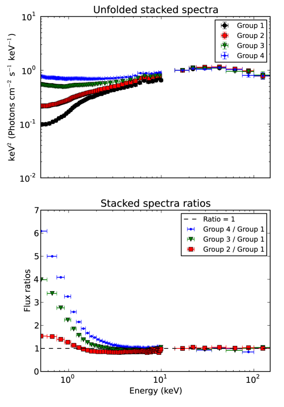
Figure 5: Results of stacking spectra per soft-excess strengths. Top panel: Unfolded stacked XMM-Newton/PN and Swift/BAT spectra for the four groups of different $q$ (normalized to the spectrum with a lower $q$ value, at 15 keV). The $q$ value is increasing for stacked spectra from black circles (Group 1) to red squares (Group 2), to green triangles (Group 3) and to blue dots (Group 4). Bottom panel: Ratios of the stacked XMM-Newton/PN and Swift/BAT spectra. The ratio of stacked spectra of higher $q$ (Group 4) over lower $q$ (Group 1) is represented in blue points. The ratio of stacked spectra from Group 3 over Group 1 is plotted in green triangles. The ratio of Group 2 over Group 1 is in red squares.

If we consider only the NLSy1s present in our sample and stack their XMM-Newton and Swift/BAT spectra for four groups of soft-excess strength, we observe the same trend as the one found for the entire sample. We see in Table 1 that the photon index is increasing for an increasing value of the soft-excess strength, but we do not note any evolution trend for the reflection factor.

7 Relation with the Eddington ratio

For 20 objects of our sample, Eddington ratios have been calculated by Ricci et al. (2013). They used average bolometric corrections $k_{x}$ (taken from the literature) obtained from studies of the AGN spectral energy distribution to calculate the Eddington ratios. Considering black-hole masses from previous works of Woo & Urry (2002) and Vasudevan et al. (2010), we can easily calculate the Eddington ratios for 13 additional objects not studied in Ricci et al. (2013). The Eddington ratio is calculated as

$$\lambda_{Edd}=\frac{L_{Bol}}{L_{Edd}}=\frac{k_{x}\times L_{2-10\,keV}}{1.26\times 10^{38}\times M_{BH}/M_{\odot}}.$$ (10)

We plotted the photon index as a function of the Eddington ratio for the 33 NLSy1, Sy1, and Sy1.5 objects in Fig. 6. A linear regression with linmix_err gives the following relation:

$$\Gamma=0.13\,_{-0.04}^{+0.05}\times log(\lambda_{Edd})+1.89\,_{-0.03}^{+0.08}$$ (11)

with a correlation coefficient of 0.47 and a null-hypothesis probability of 0.4%. The instrinsic scatter of $\Gamma$ is 0.02. Such a positive correlation has already been found in several works performed using ASCA, ROSAT, Swift, and XMM-Newton (Wang et al. 2004; Grupe 2004; Porquet et al. 2004; Bian et al. 2005; Grupe et al. 2010), establishing a relation between $\Gamma$ and $\lambda_{Edd}$ (Shemmer et al. 2008; Risaliti et al. 2009; Jin et al. 2012).

In Fig. 7 we plotted the soft-excess strength as a function of the Eddington ratio. We find

$$q=0.28\,_{-0.15}^{+0.01}\times log(\lambda_{Edd})+0.72\,_{-0.09}^{+0.11}.$$ (12)

A correlation exists with a coefficient of 0.43 and is significant (null-hypothesis probability of 1%). The intrinsic scatter of $q$ is 0.07.

We plotted the reflection factor as a function of the Eddington ratio in Fig. 8. The linear regression process leads to the relation:

$$log(R)=0.06\,_{-0.08}^{+0.09}\times log(\lambda_{Edd})-0.09\,_{-0.12}^{+0.10}.$$ (13)

The correlation between $R$ and $\lambda_{Edd}$ is not significant since the correlation coefficient of 0.17 is obtained with a null-hypothesis probability of 31%. The intrinsic scatter of $log(R)$ is 0.05.

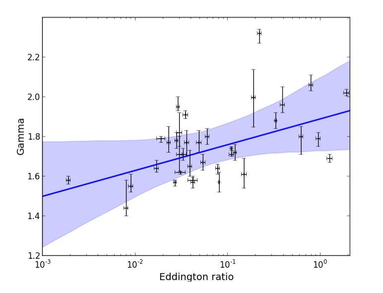
Figure 6: Photon index of the primary continuum as a function of the Eddington ratio. Linear regression is represented by the blue line and 99% CI is given by the blue contour.

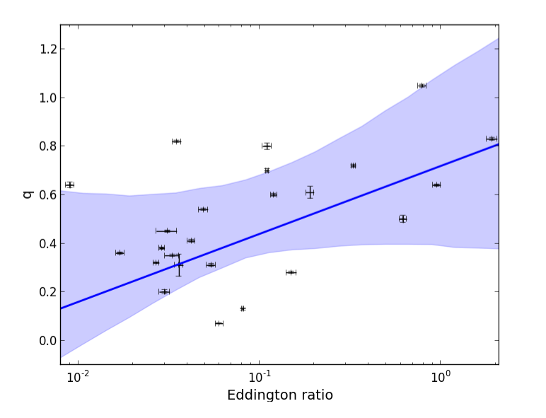
Figure 7: Soft-excess strength as a function of the Eddington ratio. Linear regression is represented by the blue line and 99% CI is given by the blue contour.

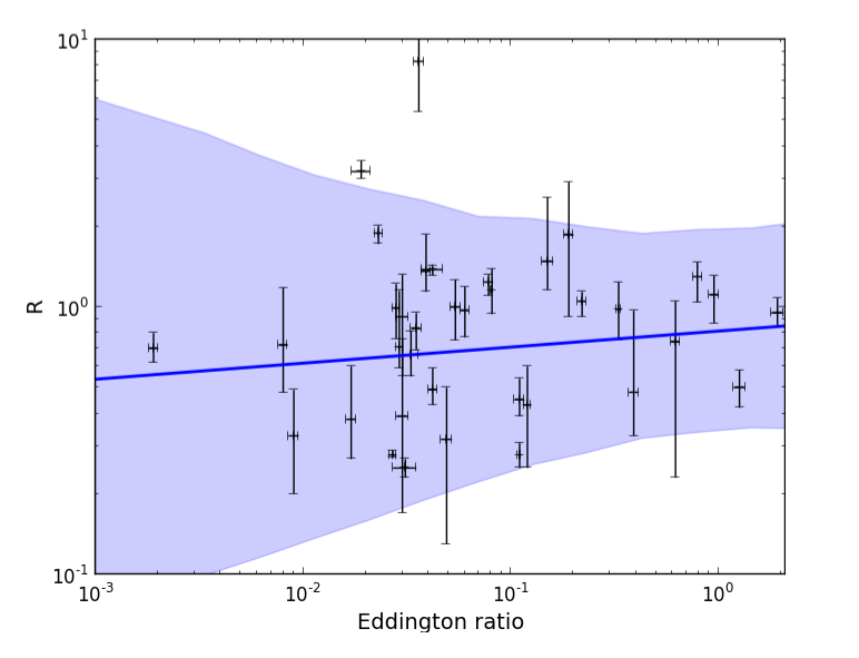
Figure 8: Reflection factor as a function of the Eddington ratio. Linear regression is represented by the blue line and 99% CI is given by the blue contour.

8 Discussion

We studied 102 Seyfert 1s (Sy1.0, 1.2, 1.5, NLSy1) from the Swift/BAT 70-Months Hard X-ray Survey catalog, using Swift/BAT and XMM-Newton observations. The simultaneous spectral analysis of the soft and the hard X-ray emission aimed to study the behavior between the soft excess present in a large number of Seyfert 1s and the reflection component. We have seen that our results are not affected by the presence of NLSy1s in our sample, because the trends are similar or compatible when excluding these objects from our analysis or when considering only NLSy1s (relations found between $q$, $R$, and $\Gamma$ and stacking of spectra). This suggests that the mechanism responsible for the soft excess is similar for all the categories of our sample. We did not find any effect of ionized absorption present in many objects of our sample. Our method of measuring the soft-excess strength is robust even in objects with moderate absorption.

8.1 Link between soft excess and reflection

Vasudevan et al. (2013) studied a sample of AGNs from the 58-month Swift/BAT catalog. Using BAT and XMM-Newton data, they constrained the reflection and the soft-excess strength in 39 sources. A plot of the reflection strength $R$ against the soft-excess strength for the 23 low-absorption sources from Vasudevan et al. (2013) is presented in Figure 1 of Vasudevan et al. (2014). The figure shows strong hints of a correlation. This correlation can be explained by the fact that, in the case of local reflection, higher reflection leads to stronger emission lines below 1 keV that are smeared in the vicinity of the supermassive black hole, inducing a larger smooth bump at low energy, the soft excess.

It is necessary to use simultaneous broad-band data in order to distinguish between mechanisms at the origin of the soft excess. In Vasudevan et al. (2014), XMM-Newton and NuSTAR simulations are done to produce a plot of the strength of the hard X-ray emission (measured by a neutral reflection model) versus the strength of the soft excess (modeled by a blackbody). This figure can be used as a diagnostic plot to determine the soft-excess production mechanism. Indeed, there is no evidence of a correlation between $R$ and the soft-excess strength in the case of ionized absorption, for example. But a correlation exists in the case of ionized reflection.

In our work, we use a larger sample than Vasudevan et al. (2014) (our sample contains $\sim$ 3.5 times more sources) to produce a plot of the reflection factor versus the soft-excess strength, but we did not obtain the same results as the similar plot of Vasudevan et al. (2014). Our work has ten objects in common with their analysis (Vasudevan et al. 2013). For four of them (NGC 4593, NGC 5548, IC 2637, and Mrk 50), $R$ and $q$ values match both studies. For four other sources (Mrk 817, KUG 1141+371, QSO B1419+480, and NGC 4235), very low $R$ and/or $q$ values from the study of Vasudevan et al. (2014) have intermediate $R$ and $q$ values in our work. For NGC 4051, we obtain a smaller reflection factor than Vasudevan et al. (2014), and non-negligible absorption prevents the detection of a soft excess. Mrk 766 gives us a similar value for the soft-excess strength, but a lower value of $R$, compared to results from Vasudevan et al. (2014). We note that, in general, reflection factors measured in our work are rarely higher than 2, as spectral fitting results from Crummy et al. (2006) and Walton et al. (2013), who obtained $R\sim 1$ on average, while Vasudevan et al. (2013) get higher $R$ values. The correlation found in Vasudevan et al. (2014) seems to be driven by objects that show extreme values of $R$ and $q$ but whose measurements are unreliable. These differences between the results can occur because Vasudevan et al. (2013) used a different fitting process. Indeed, they fitted spectra from 1.5 keV with a pexrav model, ignoring the iron energy band (between 5.5 and 7.5 keV), fixing abundances, adding an absorber to the model and using a blackbody to model the soft excess from 0.4 keV. They also used a different definition of $q$ ($L_{BB,0.4-3\,keV}/L_{pow,1.5-6\,keV}$). The cross-calibration method also differs. Indeed, Vasudevan et al. (2013) renormalized some BAT spectra for objects whose soft X-ray observations had been taken within the timeframe of the BAT survey, using the BAT light curve and considering the ratio between BAT flux during the entire survey and BAT flux during the XMM-Newton observation. However, variability in AGN can happen also on time scales shorter than a month, so this ratio might not be indicative of the real difference in flux between the short XMM-Newton observations and the 70-month averaged Swift/BAT flux.

After analyzing our sample of objects spectrally, we do not see any hint of correlation as found in the plot of the reflection versus the soft-excess strength of Vasudevan et al. (2014). We even find evidence of a weak anti-correlation between $R$ and $q$ (see blue contours in top panel of Fig. 2). We used the relxilllp_ion model to simulate spectra, as we measure $q$ and $R$ differently than in the work of Vasudevan et al. (2014). Our simulations are in good agreement with those carried out by Vasudevan et al. (2014). Indeed, as reported by Vasudevan et al. (2014), if the soft excess was entirely due to blurred reflection, one would expect to find a correlation between the reflection factor and the soft-excess strength (see red line in top panel of Fig. 2). In this case, we should obtain high $R$ and high $q$, as well as small $R$ and small $q$ ($R<2.0$ and $q<0.75$, blue box in bottom panel of Fig. 2). That most of the objects of our sample (75%) appear in the blue box is difficult to explain in the blurred ionized-reflection hypothesis, because this model predicts that only 25% of the objects should appear as small-$q$, small-$R$. There is no easy way to restrict the parameter space to match the blue box. In particular, high-$R$, high-$q$ objects are objects with intermediate ionization. Considering our sample of 79 Seyfert 1s, no positive correlation is found between $R$ and $q$ (both in the local and in the distant reflection scenarii) and only low $R$ and $q$ values are measured (see bottom panel of Fig. 2). These contradictions are a strong argument against the ionized-reflection hypothesis as the origin of the soft excess in most objects.

By stacking XMM-Newton/PN and Swift/BAT spectra in different bins of soft-excess intensity (see Fig. 5), we have seen that there is no obvious difference in the spectral shape in the hard X-ray band in the individual stacked spectra and in their ratios. In stacked spectra with the lower soft-excess strength values, absorption can be seen below 1 keV (see black circles and red squares in Fig. 5), as many objects of our sample are slightly absorbed. For higher values of the soft-excess intensity (see green triangles and blue points of Fig. 5), the soft-excess emission compensates for and dominates the absorption, assuming that absorption is equally present in each of the four groups of soft-excess strength. While the spectra are steeper for a stronger soft excess, we do not see any evolution of the reflection factor. We observe the same results when only stacking NLSy1 spectra. The values of the photon index we obtain are consistent with those found by Ricci et al. (2011) by stacking INTEGRAL spectra of type 1 and 1.5 AGN. There is no stronger reflection feature in the hard X-ray band for stronger soft excess, since we would expect in the case where ionized reflection is at the origin of the soft excess. This result suggests that the blurred ionized reflection is not responsible for the existence of the soft excess in most objects of our sample.

8.2 Soft excess and X-ray continuum

Studying our 79 objects with soft excess, we found a possible correlation between the photon index of the primary continuum and the strength $q$ of the soft excess (see blue contours in Fig. 3). This trend is also verified when we consider the objects grouped per soft-excess strength, by fitting spectra stacked per soft-excess strengths (see Table 1). Such a correlation has already been cautiously presented in Page et al. (2004b) with a higher significance than in this work. A possible faint anti-correlation between $\Gamma$ and $q$ is expected in the case of ionized reflection, as shown by relxilllp_ion simulations (see red line and contours in Fig. 3), which is at odds with the possible positive correlation found with our data. A positive correlation like the one found in our sample might suggest a connection between the soft excess and the cooling of the hot corona. As proposed in the case of Mrk 509 (Petrucci et al. 2013), a warm corona could upscatter the optical-UV photons from the accretion disk to produce the soft excess. This soft excess could constitute a non-negligible part of the soft photons Comptonized in the hot corona (producing the primary X-ray continuum), since they would participate in its cooling. Indeed, the warm plasma emission peaks from a few eV to a few hundred eV, so it could be considered by the hot corona as a soft photon field with an intermediate temperature (see Figure 10 in Petrucci et al. 2013). The geometry of a hot photon-starved corona surrounded by an outer cold disk has already been suggested by Abramowicz et al. (1995) and Narayan & Yi (1995) and applied, for example, in NGC 4151 by Lubiński et al. (2010). Petrucci et al. (2013) propose that the plasma responsible for the soft excess in Mrk 509 could be a warm upper layer of this accretion disk. In this case, a higher soft-excess strength $q$ means a more efficient cooling and a softer X-ray emission. The relation between $\Gamma$ and $q$ is an argument in favor of warm Comptonization models to explain the soft excess.

Studying the relation between $R$ and $\Gamma$, we found a correlation with our 79 objects (see blue contours in Fig. 4). A faint correlation is also expected with ionized reflection (see red contours in Fig. 4), but the relation slopes are different. The mean value of $R\sim 5$ for the ionized reflection is due to the chosen parameters for the simulations. Indeed, we chose a reflection factor going up to 100 for the relxilllp_ion model, so the reflection factor R measured with pexmon is high. But this mean value of $R\sim 5$ resulting from simulations does not have a real meaning because the values of the other parameters are not known. Correlations have been found previously between the reflection and the power-law photon index in several works. Using Ginga spectra of radio-quiet Seyfert 1s and narrow emission-line galaxies, Zdziarski et al. (1999) found a very strong correlation between the intrinsic spectral slope in X-rays and the amount of Compton reflection from a cold medium ($R\propto\Gamma^{12}$). They interpreted this as due to a feedback within the source where the cold medium responsible for the reflection emits soft photons that irradiate the X-ray source and participate in the cooling as seeds for Compton upscattering. Fainter correlations have also been found between $R$ and $\Gamma$ and between the spectral slope and the strength of the iron line (Lubiński & Zdziarski 2001; Perola et al. 2002). Mattson et al. (2007) found a relation between $R$ and $\Gamma$ ($R=0.54\Gamma-0.87$), close to the one we found during our analysis ($R=1.07\,_{-0.37}^{+0.76}\times\Gamma-1.11\,_{-1.34}^{+0.62}$), which could be due to degeneracies during modeling process. According to Malzac & Petrucci (2002), the correlation between $R$ and $\Gamma$ could be due to the presence of a remote cold material. Indeed, assuming that disk reflection is negligible and thus that reflection is mainly due to distant cold material, fluctuations in the primary X-ray emission slope at constant flux make the spectrum pivot, inducing a correlation between $\Gamma$ and $R$. The correlation between $R$ and $\Gamma$ that we find for both local and distant reflection scenarii, because it differs from blurred ionized-reflection model expectations in slope, is another argument against the ionized-reflection hypothesis as the origin of the soft excess.

8.3 Relations with the Eddington ratio $\lambda_{Edd}$

A positive correlation has already been found between the photon index of the primary continuum and the Eddington ratio in several works (Wang et al. 2004; Grupe 2004; Porquet et al. 2004; Bian et al. 2005; Kelly 2007; Shemmer et al. 2008; Risaliti et al. 2009; Grupe et al. 2010; Jin et al. 2012). Shemmer et al. (2008) found the relation $\Gamma=0.31\,log(\lambda_{Edd})\,+\,2.11$, consistent with results from Wang et al. (2004) and Kelly (2007). Risaliti et al. (2009) and Jin et al. (2012) find a steeper relation: $\Gamma\propto 0.60\,log(\lambda_{Edd})$. This relation implies a link between the accretion disk and the hot corona that could be due to the fact that the more accretion disk emits optical/UV photons, the more efficient the cooling of the corona. With our sample of 79 Seyfert 1s, we possibly found such a correlation between $\Gamma$ and $\lambda_{Edd}$ (see Fig. 6), with a flatter relation that is inconsistent with previous results ($\Gamma=0.13\,log(\lambda_{Edd})+1.89$). The difference between our result and previous ones may be due to the different fitting procedures, because Shemmer et al. (2008), Risaliti et al. (2009) and Jin et al. (2012) used a simple absorbed power law to fit their data.

As shown in Fig. 7, we found a possible correlation between $\lambda_{Edd}$ and $q$. This might show a link between the accretion disk and the warm corona responsible for the soft excess in the warm Comptonization model. In the case of Mrk 509, Petrucci et al. (2013) propose a geometry where the warm corona is the top layer of the accretion disk. The warm corona heats the deeper layers and Comptonizes their optical/UV photons, creating the soft-excess feature (see Figure 10 in Petrucci et al. 2013). Such a geometry could then explain the correlation between $\lambda_{Edd}$ and $q$, which is an argument in favor of the warm Comptonization hypothesis as the origin of the soft excess. Since we find correlations between $\lambda_{Edd}$ and $q$ and between $\Gamma$ and $\lambda_{Edd}$, a correlation between $\Gamma$ and $q$, such as the one found in Sect. 5.1, is expected, driven by $\lambda_{Edd}$.

The Baldwin effect, which is an anti-correlation between the equivalent width (EW) of the iron K$\alpha$ line and the X-ray luminosity ($EW\propto L_{X}^{-0.20}$ – Iwasawa & Taniguchi 1993), could be explained by the decrease in luminosity when the covering factor of the torus from the unification model increases (Page et al. 2004a; Bianchi et al. 2007). A similar trend has been observed between the EW of the FeK$\alpha$ line and the Eddington ratio. Studying a large sample of unabsorbed AGN, Bianchi et al. (2007) found the relation $EW\propto\lambda_{Edd}^{-0.19}$, while Shu et al. (2010) used a sample of Chandra/HEG observations to find a similar relation of $EW\propto(L_{2-10\,keV}/L_{Edd})^{-0.20}$ when fitting each observation, but a weaker correlation ($EW\propto(L_{2-10\,keV}/L_{Edd})^{-0.11}$) when doing the fits per source. Using results of Shu et al. (2010) and bolometric corrections, Ricci et al. (2013) found the relation $log(EW)=-0.13\,log(\lambda_{Edd})+1.47$.

We found, in our work, an anti-correlation between $R$ and $q$. We also found a positive correlation between $q$ and $\lambda_{Edd}$. We then expect to have an anti-correlation between $R$ and $\lambda_{Edd}$, which is similar to the Baldwin effect, since the EW of the Fe K$\alpha$ line and the reflection factor $R$ are both representative of the reflection strength. Unfortunately, this expected anti-correlation between $R$ and $\lambda_{Edd}$ is not seen in our sample, probably because of intrinsic scatter and large uncertainties.

A possible explanation for this anti-correlation between $R$ and $q$ is the warm Comptonization. In this scenario, a warm plasma, which could be the upper layer of the disk, upscatters the soft optical/UV photons from the disk to reproduce the soft excess. Since the warm plasma at a temperature of $\sim$ 1 keV is highly ionized, reflection on this medium is largely featureless and follows the primary emission. Therefore, a disk covered with a warm plasma sees its reflection factor $R$ decrease compared to the case with little warm plasma or none at all. As a result, the stronger the soft excess, the smaller the reflection factor. The anti-correlation found in data between $R$ and $q$ could then be explained if the soft excess came from a warm plasma.

9 Conclusion

The nature of the soft excess in AGN is still uncertain because physical mechanisms used to model this feature are difficult to distinguish when analyzing soft X-rays spectra. The Swift/BAT and XMM-Newton spectral analysis of a large sample of Seyfert 1s from the Swift/BAT 70-Months Hard X-ray Survey catalog allowed a hard X-ray view of the soft excess in AGN. We fit the 3-100 keV data with phenomenological model and then quantify the soft excess below 2 keV with respect to this model. We found that 80% of the objects of our sample show the presence of a soft excess.

Fitting the spectra of 79 Seyfert 1s lowly absorbed and showing a soft excess, we showed that the soft-excess strength and the reflection factor are not positively correlated. By stacking XMM-Newton/PN and Swift/BAT spectra per soft-excess strengths, we have shown that the reflection characterized by the Compton hump at about 30 keV does not vary with the soft-excess strength. These results contradict the correlation expected from ionized reflection, as shown by our simulations with relxilllp_ion and by simulations of XMM-Newton and NuSTAR spectra from Vasudevan et al. (2014). This contradiction between expectations and measurements is a strong argument against the ionized-reflection hypothesis as the origin of the soft excess in most objects. The possible anti-correlation we found could be explained by a warm Comptonization scenario, where a warm plasma covering the disk would make the reflection featureless.

We have also seen that the strength of the soft excess $q$ is correlated with the spectral index $\Gamma$ and with the Eddington ratio $\lambda_{Edd}$. This could be explained by warm Comptonization scenarii, such as the one described in Petrucci et al. (2013), where a higher $q$ value might mean a more efficient cooling of the hot corona responsible for the primary X-ray emission and hence a steeper spectrum. Furthermore, the relation found between $R$ and $\Gamma$ is different from the one found in relxilllp_ion simulations and can be used as an additional argument against ionized reflection. The correlation could be because the medium responsible for reflection emits soft photons that participate in the cooling of the hot corona.

The relation found between $R$, $\Gamma$, and $q$ are found when assuming a reflection component mainly due to distant material, as well as if this reflection mainly comes from the accretion disk, which we cannot distinguish here.

This work suggests that the soft excess present in 80% of the objects of our sample is, in most cases, likely not due to blurred ionized reflection, but can most probably be explained by warm Comptonization. Future works with NuSTAR and ASTRO-H will shed light on this issue, as the better signal-to-noise data they will provide in the hard X-ray band may allow both models to be spectrally distinguished.

Table 2: List of the sources used for this study, with their spectral types, redshifts $z$, Galactic column densities ($N_{\rm\,H}^{\rm\,G}$ values from Dickey & Lockman (1990)), and soft X-ray observations information (observation date, observation identification and net exposure).

Source	Type	z	$N_{\rm\,H}^{\rm\,G}$	Obs. date	Obs. ID	Net exposure
			[$10^{20}\rm\,cm^{-2}$]	YYYY-MM-DD		[$\rm\,ks$]
1H 0419$-$577	Sy 1.5	0.104	1.83	2010$-$05$-$30	0604720301	100.3
1H 2251$-$179P	Sy 1.5	0.064	2.7	2002$-$05$-$18	0012940101	61.8
1RXS J213944.3+595016	Sy 1.5	0.114	59.7	2008$-$05$-$11	0555321001	8.7
2MASSi J1031543$-$141651	Sy 1.0	0.086	6.45	2004$-$12$-$19	0203770101	34.6
2MASX J18560128+1538059	Sy 1.0	0.084	37.4	2009$-$04$-$06	0550451601	6.2
2MASX J22484165$-$5109338	Sy 1.5	0.100	1.35	2007$-$05$-$15	0510380101	64.5
3C 111.0	Sy 1.0	0.048	32.2	2009$-$02$-$15	0552180101	71.8
3C 382	Sy 1.0	0.058	7.46	2008$-$04$-$28	0506120101	32.4
3C 390.3	Sy 1.5	0.056	4.28	2004$-$10$-$08	0203720201	51.7
4C +74.26	Sy 1.0	0.104	12.2	2004$-$02$-$06	0200910201	31.9
4U 0517+17	Sy 1.5	0.018	22.0	2007$-$08$-$21	0502090501	57.2
6dF J2132022$-$334254P	Sy 1.2	0.030	4.07	2004$-$10$-$30	0201130301	46.0
Ark 120	Sy 1.0	0.032	12.6	2003$-$08$-$25	0147190101	105.3
CGCG 229$-$015	Sy 1.0	0.028	6.25	2011$-$06$-$05	0672530301	23.9
ESO 140$-$43	Sy 1.5	0.014	7.3	2005$-$09$-$08	0300240401	21.8
ESO 141$-$55P	Sy 1.2	0.037	5.1	2007$-$10$-$30	0503750101	77.6
ESO 198$-$024	Sy 1.0	0.046	3.05	2006$-$02$-$04	0305370101	121.9
ESO 209$-$12	Sy 1.5	0.040	23.8	2006$-$03$-$25	0401790301	7.2
ESO 323$-$77	Sy 1.2	0.015	7.4	2006$-$02$-$07	0300240501	25.6
ESO 359$-$ G 019	Sy 1.0	0.055	1.02	2004$-$03$-$09	0201130101	24.0
ESO 548$-$G081P	Sy 1.0	0.014	3.04	2006$-$01$-$28	0312190601	10.0
EXO 055620$-$3820.2	Sy 1.2	0.034	4.0	2006$-$11$-$03	0404260301	75.9
Fairall 1116	Sy 1.0	0.058	3.09	2005$-$08$-$28	0301450301	20.1
Fairall 1146	Sy 1.0	0.032	40.3	2006$-$12$-$12	0401790401	11.6
Fairall 9	Sy 1.2	0.047	3.28	2009$-$12$-$09	0605800401	129.6
GQ Com	Sy 1.2	0.165	1.67	2002$-$05$-$30	0109080101	13.3
GRS 1734$-$292P	Sy 1.0	0.021	76.7	2009$-$02$-$26	0550451501	12.1
$[$HB89$]$ 0052+251	Sy 1.2	0.154	4.93	2005$-$06$-$26	0301450401	19.8
$[$HB89$]$ 0119$-$286	Sy 1.0	0.116	1.65	2003$-$01$-$07	0110950201	5.7
$[$HB89$]$ 0241+622	Sy 1.2	0.044	74.2	2008$-$02$-$28	0503690101	30.0
IC 0486	Sy 1.0	0.027	3.95	2007$-$10$-$28	0504101201	20.1
IC 2637	Sy 1.5	0.029	2.66	2009$-$12$-$20	0601780201	13.2
IC 4329A	Sy 1.2	0.016	4.4	2003$-$08$-$06	0147440101	118.4
IGR J00335+6126	Sy 1.5	0.105	61.6	2010$-$01$-$15	0601740101	21.5
IGR J07597$-$3842	Sy 1.2	0.040	60.3	2006$-$04$-$08	0303230101	15.0
IGR J11457$-$1827	Sy 1.5	0.033	3.5	2004$-$06$-$08	0201130201	31.0
IGR J12172+0710	Sy 1.2	0.008	1.5	2004$-$06$-$09	0204650201	9.3
IGR J13038+5348P	Sy 1.2	0.029	1.6	2006$-$06$-$23	0312192001	9.6
IGR J13109$-$5552	Sy 1.0	0.104	27.6	2009$-$02$-$26	0550450901	17.9
IGR J16119$-$6036	Sy 1.5	0.016	23.1	2009$-$02$-$18	0550451101	13.1
IGR J16185$-$5928	NLSy 1	0.035	24.7	2009$-$02$-$18	0550451201	17.4
IGR J16482$-$3036	Sy 1.0	0.031	17.6	2006$-$03$-$01	0305831001	7.5
IGR J16558$-$5203	Sy 1.2	0.054	30.4	2006$-$03$-$01	0306171201	8.9
IGR J17418$-$1212	Sy 1.2	0.037	20.9	2006$-$04$-$04	0303230501	13.1
IGR J17488$-$3253	Sy 1.0	0.020	53.0	2007$-$03$-$03	0405390101	6.57
IGR J18027$-$1455	Sy 1.0	0.035	49.7	2006$-$03$-$25	0303230601	18.1
IGR J18259$-$0706	Sy 1.0	0.037	71.2	2011$-$03$-$07	0650591501	25.9
IGR J19378$-$0617	Sy 1.5	0.011	14.8	2009$-$04$-$28	0550451701	17.4
IGR J21277+5656	NLSy 1	0.015	78.7	2010$-$11$-$29	0655450101	127.5
IRAS 04392$-$2713	Sy 1.5	0.084	2.49	2005$-$08$-$13	0301450101	20.0
IRAS 15091$-$2107	NLSy 1	0.044	8.42	2005$-$07$-$26	0300240201	18.7
KUG 1141+371	Sy 1.0	0.038	1.90	2009$-$05$-$23	0601780501	5.4
LEDA 168563	Sy 1.0	0.029	54.2	2007$-$02$-$26	0401790201	10.5
MCG $-$02$-$14$-$009	Sy 1.0	0.028	9.23	2009$-$02$-$27	0550640101	79.1
MCG$-$02$-$58$-$022	Sy 1.5	0.047	3.60	2000$-$12$-$01	0109130701	10.3
MCG$-$06$-$30$-$015	Sy 1.5	0.008	4.08	2001$-$08$-$04	0029740801	124.0
MCG+08$-$11$-$011	Sy 1.5	0.020	20.9	2004$-$04$-$09	0201930201	30.4
Mrk 1040	Sy 1.0	0.016	7.22	2009$-$02$-$13	0554990101	66.8
Mrk 1044	NLSy 1	0.016	3.36	2013$-$01$-$27	0695290101	107.2
Mrk 110	NLSy 1	0.035	1.47	2004$-$11$-$15	0201130501	47
Mrk 1152	Sy 1.5	0.052	1.68	2003$-$06$-$15	0147920101	21.5
Mrk 279	Sy 1.0	0.030	1.78	2005$-$11$-$17	0302480501	49.2
Mrk 290	Sy 1.5	0.030	1.70	2006$-$05$-$06	0400360801	18.6
Mrk 335	NLSy 1	0.026	4.03	2006$-$01$-$03	0306870101	117.0
Mrk 352P	Sy 1.0	0.015	5.59	2006$-$01$-$24	0312190101	10.8
Mrk 359	NLSy 1	0.017	4.79	2010$-$07$-$25	0655590201	24.8
Mrk 50	Sy 1.2	0.024	1.77	2010$-$12$-$09	0650590401	15.7
Mrk 509	Sy 1.5	0.034	4.11	2006$-$04$-$25	0306090401	61.8
Mrk 590	Sy 1.0	0.027	2.68	2004$-$07$-$04	0201020201	32.4
Mrk 6	Sy 1.5	0.019	6.39	2001$-$03$-$27	0061540101	26.0
Mrk 684P	NLSy 1	0.046	1.46	2006$-$01$-$24	0300910101	11.1
Mrk 704	Sy 1.2	0.029	3.43	2008$-$11$-$02	0502091601	87.0
Mrk 739E	NLSy 1	0.029	1.90	2009$-$06$-$14	0601780401	10.0
Mrk 766	NLSy 1	0.013	1.71	2001$-$05$-$20	0109141301	121.4
Mrk 771	Sy 1.0	0.063	2.24	2005$-$07$-$09	0301450201	24.3
Mrk 79	Sy 1.2	0.022	5.73	2008$-$04$-$26	0502091001	67.6
Mrk 817P	Sy 1.5	0.031	1.49	2009$-$12$-$13	0601781401	5.6
NGC 3227	Sy 1.5	0.004	2.15	2006$-$12$-$03	0400270101	101.3
NGC 3516	Sy 1.5	0.009	3.05	2001$-$11$-$09	0107460701	119.5
NGC 3783	Sy 1.5	0.010	8.50	2001$-$12$-$19	0112210501	127.5
NGC 4051	NLSy 1	0.002	1.32	2002$-$11$-$22	0157560101	48.2
NGC 4151	Sy 1.5	0.003	1.98	2000$-$12$-$22	0112830201	57.0
NGC 4593	Sy 1.0	0.009	2.31	2000$-$07$-$02	0109970101	10.1
NGC 5548	Sy 1.5	0.017	1.69	2001$-$07$-$09	0089960301	70.2
NGC 6814	Sy 1.5	0.005	12.8	2009$-$04$-$22	0550451801	28.4
NGC 7469	Sy 1.5	0.016	4.87	2004$-$11$-$30	0207090101	84.5
NGC 7603	Sy 1.5	0.030	4.09	2006$-$06$-$14	0305600601	16.4
NGC 985	Sy 1.5	0.043	2.9	2003$-$07$-$15	0150470601	57.6
PG 0804+761	Sy 1.0	0.100	2.98	2010$-$03$-$10	0605110101	42.8
PG 1501+106	Sy 1.5	0.036	2.34	2005$-$01$-$16	0205340201	46
PKS 0558$-$504	NLSy 1	0.137	4.50	2008$-$09$-$11	0555170401	123.3
PKS 2135$-$14	Sy 1.5	0.200	4.70	2001$-$04$-$28	0092850201	27.2
QSO B1419+480	Sy 1.5	0.072	1.65	2002$-$05$-$27	0094740201	20.1
QSO B1821+643	Sy 1.2	0.297	4.04	2007$-$12$-$10	0506210101	13.6
RHS 39	Sy 1.0	0.022	4.88	2007$-$08$-$05	0502090201	108.9
RX J2135.9+4728	Sy 1.0	0.025	38.6	2010$-$11$-$11	0650591701	22.8
SWIFT J0519.5$-$3140	Sy 1.0	0.013	1.76	2010$-$01$-$29	0610180101	76.5
SWIFT J0640.4$-$2554	Sy 1.0	0.026	11.4	2006$-$03$-$07	0312190801	10.3
SWIFT J0917.2$-$6221	Sy 1.0	0.057	19.1	2008$-$12$-$14	0550452601	16
SWIFT J1038.8$-$4942	Sy 1.0	0.060	27.2	2011$-$01$-$11	0650591101	24.9
SWIFT J2009.0$-$6103	Sy 1.5	0.015	4.2	2009$-$03$-$30	0552170301	92.9
UGC 3142	Sy 1.0	0.022	19.0	2007$-$03$-$18	0401790101	9.8
P source presented pile-up and the extraction region used is an annulus of inner radius 15 arcsec

Table 3: EPIC-PN and MOS XMM-Newton and Swift/BAT data analysis.

Source	$\Gamma$	$F_{\text{continuum}}$ (2-10)	$F_{\text{soft excess}}$ (0.5-2)	Model	$q$	R	$\chi^{2}$/dof
		$10^{-11}\rm\,erg\,cm^{-2}\,s^{-1}$	$10^{-11}\rm\,erg\,cm^{-2}\,s^{-1}$
1H 0419$-$577	$1.79\,_{-0.04}^{+0.03}$	$1.08\,_{-0.002}^{+0.002}$	$0.43\,_{-0.003}^{+0.003}$	2brem	$0.64\,_{-0.005}^{+0.005}$	$1.11\,_{-0.24}^{+0.20}$	4347/3996
1H2251$-$179	$1.57\,_{-0.05}^{+0.05}$	$1.87\,_{-0.004}^{+0.004}$	$0.11\,_{-0.003}^{+0.003}$	1brem + WA	$0.13\,_{-0.004}^{+0.004}$	$1.15\,_{-0.21}^{+0.24}$	3378/3199
1RXSJ213944.3+595016	$1.69\,_{-0.05}^{+0.09}$	$0.55\,_{-0.005}^{+0.005}$	–	Absorbed	–	$0.27\,_{-0.14}^{+0.46}$	654/643
2MASSi J1031543$-$141651	$1.73\,_{-0.02}^{+0.03}$	$1.58\,_{-0.004}^{+0.004}$	$0.79\,_{-0.01}^{+0.01}$	2brem	$0.82\,_{-0.011}^{+0.011}$	$0.38\,_{-0.08}^{+0.09}$	3039/3044
2MASX J18560128+1538059	$1.73\,_{-0.07}^{+0.12}$	$1.03\,_{-0.005}^{+0.005}$	$0.10\,_{-0.007}^{+0.007}$	Cold abs + 1brem	$0.17\,_{-0.012}^{+0.012}$	$1.01\,_{-0.33}^{+0.64}$	1489/1540
2MASX J22484165$-$5109338	$1.64\,_{-0.06}^{+0.09}$	$0.38\,_{+0.0009}^{+0.0009}$	$0.10\,_{-0.002}^{+0.002}$	2brem	$0.53\,_{-0.011}^{+0.011}$	$0.79\,_{-0.33}^{+0.47}$	2202/2195
3C 111.0	$1.54\,_{-0.02}^{+0.02}$	$3.92\,_{-0.005}^{+0.005}$	$0.29\,_{-0.006}^{+0.006}$	Cold abs + 1brem	$0.17\,_{-0.004}^{+0.004}$	$0.15\,_{-0.10}^{+0.09}$	3430/3147
3C 382	$1.77\,_{-0.05}^{+0.06}$	$3.48\,_{-0.006}^{+0.006}$	$1.14\,_{-0.01}^{+0.01}$	2brem + WA	$0.54\,_{-0.005}^{+0.005}$	$0.32\,_{-0.19}^{+0.18}$	2794/2652
3C 390.3	$1.57\,_{-0.02}^{+0.01}$	$3.43\,_{-0.007}^{+0.007}$	$0.52\,_{-0.006}^{+0.006}$	2brem + WA	$0.32\,_{-0.004}^{+0.004}$	$0.28\,_{-0.007}^{+0.01}$	4863/4349
4C +74.26	$1.78\,_{-0.04}^{+0.04}$	$1.83\,_{-0.003}^{+0.003}$	–	Absorbed	–	$0.99\,_{-0.23}^{+0.23}$	4069/3680
4U 0517+17	$1.67\,_{-0.05}^{+0.05}$	$2.31\,_{-0.004}^{+0.004}$	$0.10\,_{-0.002}^{+0.002}$	1brem + WA	$0.08\,_{-0.002}^{+0.002}$	$1.01\,_{-0.19}^{+0.21}$	4789/4062
6dF J2132022$-$334254	$1.42\,_{-0.05}^{+0.13}$	$0.79\,_{-0.004}^{+0.004}$	$0.09\,_{-0.003}^{+0.003}$	2brem	$0.32\,_{-0.011}^{+0.011}$	$0.64\,_{-0.21}^{+0.52}$	2167/2193
Ark 120	$1.91\,_{-0.02}^{+0.02}$	$2.97\,_{-0.003}^{+0.003}$	$1.83\,_{-0.008}^{+0.008}$	2brem	$0.82\,_{-0.004}^{+0.004}$	$0.83\,_{-0.14}^{+0.12}$	5219/4654
CGCG 229$-$015	$1.72\,_{-0.12}^{+0.15}$	$0.32\,_{-0.001}^{+0.001}$	$0.08\,_{-0.003}^{+0.003}$	2brem	$0.44\,_{-0.017}^{+0.017}$	$0.96\,_{-0.59}^{+0.79}$	1520/1567
ESO 140$-$43	$1.97\,_{-0.05}^{+0.04}$	$1.80\,_{-0.004}^{+0.004}$	–	2brem + WA	–	$2.15\,_{-0.40}^{+0.28}$	2906/2570
ESO 141$-$55	$1.95\,_{-0.02}^{+0.05}$	$2.82\,_{-0.006}^{+0.006}$	$0.85\,_{-0.01}^{+0.01}$	2brem	$0.38\,_{-0.005}^{+0.005}$	$0.71\,_{-0.12}^{+0.44}$	3230/2789
ESO 198$-$024	$1.64\,_{-0.02}^{+0.04}$	$0.81\,_{-0.001}^{+0.001}$	$0.15\,_{-0.002}^{+0.002}$	2brem	$0.36\,_{-0.005}^{+0.005}$	$0.38\,_{-0.11}^{+0.22}$	2875/2780
ESO 209$-$12	$1.68\,_{-0.05}^{+0.08}$	$0.68\,_{-0.005}^{+0.005}$	$0.25\,_{-0.006}^{+0.006}$	1brem + WA	$0.68\,_{-0.017}^{+0.017}$	$1.14\,_{-0.32}^{+0.70}$	1075/1034
ESO 323$-$77	–	–	–	Clumpy torus + BLR${}^{\text{(a)}}$	–	–	–
ESO 359$-$ G 019	$1.51\,_{-0.06}^{+0.04}$	$0.25\,_{-0.002}^{+0.002}$	$0.05\,_{-0.004}^{+0.004}$	2brem	$0.49\,_{-0.039}^{+0.039}$	$0.79\,_{-0.16}^{+0.53}$	1013/1012
ESO 548$-$G081	$1.55\,_{-0.03}^{+0.06}$	$1.18\,_{-0.008}^{+0.008}$	$0.50\,_{-0.009}^{+0.009}$	1brem + WA	$0.64\,_{-0.012}^{+0.012}$	$0.33\,_{-0.13}^{+0.16}$	1055/1024
EXO 055620$-$3820.2	–	–	–	Ionized absorber${}^{\text{(b)}}$	–	–	–
Fairall 1116	$1.79\,_{-0.04}^{+0.09}$	$0.60\,_{-0.003}^{+0.003}$	$0.18\,_{-0.006}^{+0.006}$	2brem	$0.48\,_{-0.016}^{+0.016}$	$0.41\,_{-0.11}^{+0.54}$	1593/1559
Fairall 1146	$2.07\,_{-0.08}^{+0.07}$	$0.80\,_{-0.006}^{+0.006}$	–	1brem + WA	–	$3.08\,_{-0.71}^{+0.62}$	1633/1583
Fairall 9	$1.71\,_{-0.03}^{+0.03}$	$1.64\,_{-0.002}^{+0.002}$	$0.32\,_{-0.004}^{+0.004}$	2brem	$0.35\,_{-0.004}^{+0.004}$	$0.66\,_{-0.11}^{+0.15}$	3396/2997
GQ Com	$1.62\,_{-0.08}^{+0.13}$	$0.41\,_{-0.004}^{+0.004}$	$0.09\,_{-0.003}^{+0.003}$	2brem	$0.45\,_{-0.016}^{+0.016}$	$0.16\,_{-0.16}^{+0.49}$	649/604
GRS 1734$-$292	$1.70\,_{-0.02}^{+0.04}$	$5.28\,_{-0.02}^{+0.02}$	–	Absorbed	–	$0.19\,_{-0.10}^{+0.14}$	2033/1971
[HB89] 0052+251	$1.62\,_{-0.04}^{+0.09}$	$0.57\,_{-0.003}^{+0.003}$	$0.29\,_{-0.007}^{+0.007}$	2brem	$1.03\,_{-0.025}^{+0.025}$	$0.26\,_{-0.21}^{+0.35}$	1580/1635
[HB89] 0119$-$286	$1.84\,_{-0.10}^{+0.07}$	$0.41\,_{-0.007}^{+0.007}$	$0.22\,_{-0.01}^{+0.01}$	2brem	$0.79\,_{-0.038}^{+0.038}$	$2\times 10^{-6}\,_{-2\times 10^{-6}}{}^{+0.22}$	404/410
[HB89] 0241+622	$1.60\,_{-0.06}^{+0.06}$	$1.89\,_{-0.004}^{+0.004}$	$0.17\,_{-0.004}^{+0.004}$	Cold abs + 1brem	$0.19\,_{-0.005}^{+0.005}$	$0.95\,_{-0.27}^{+0.27}$	3635/3507
IC 0486	$1.57\,_{-0.11}^{+0.16}$	$0.43\,_{-0.004}^{+0.004}$	–	2WA	–	$1.47\,_{-0.22}^{1.16}$	840/709
IC 2637	$1.62\,_{-0.08}^{+0.16}$	$0.36\,_{-0.003}^{+0.003}$	$0.04\,_{-0.0009}^{+0.0009}$	1brem	$0.23\,_{-0.005}^{+0.005}$	$0.52\,_{-0.23}^{1.00}$	861/889
IC 4329A	$1.69\,_{-0.02}^{+0.02}$	$8.17\,_{-0.006}^{+0.006}$	–	3WA + Abs + 1brem${}^{\text{(c)}}$	–	$0.50\,_{-0.08}^{+0.08}$	7521/5093
IGR J00335+6126	$1.88\,_{-0.11}^{+0.15}$	$0.29\,_{-0.003}^{+0.003}$	–	Cold abs + 1brem	–	$5.94\,_{-1.64}^{3.39}$	898/778
IGR J07597$-$3842	$1.63\,_{-0.05}^{+0.08}$	$1.38\,_{-0.006}^{+0.006}$	$0.11\,_{-0.01}^{+0.01}$	1brem + WA	$0.16\,_{-0.02}^{+0.02}$	$0.82\,_{-0.20}^{+0.44}$	2102/2130
IGR J11457$-$1827	$1.66\,_{-0.01}^{+0.01}$	$2.30\,_{-0.005}^{+0.005}$	$1.31\,_{-0.01}^{+0.01}$	2brem	$1.09\,_{-0.009}^{+0.009}$	$0.16\,_{-0.03}^{+0.04}$	2736/2533
IGR J12172+0710	$1.49\,_{-0.11}^{+0.09}$	$0.53\,_{-0.006}^{+0.006}$	$0.03\,_{-0.001}^{+0.001}$	Cold abs + 1brem	$0.14\,_{-0.005}^{+0.005}$	$0.58\,_{-0.25}^{+0.28}$	538/550
IGR J13038+5348	$1.58\,_{-0.02}^{+0.02}$	$1.21\,_{-0.006}^{+0.006}$	$0.21\,_{-0.009}^{+0.009}$	2brem	$0.39\,_{-0.02}^{+0.02}$	$0.12\,_{-0.05}^{+0.07}$	1790/1764
IGR J13109$-$5552	$1.37\,_{-0.06}^{+0.04}$	$0.47\,_{-0.003}^{+0.003}$	$0.06\,_{-0.003}^{+0.003}$	1brem	$0.39\,_{-0.02}^{+0.02}$	$4\times 10^{-9}\,_{-4\times 10^{-9}}{}^{+0.5}$	1167/1159
IGR J16119$-$6036	$1.70\,_{-0.12}^{+0.05}$	$0.60\,_{-0.004}^{+0.004}$	$0.09\,_{-0.007}^{+0.007}$	2brem	$0.27\,_{-0.02}^{+0.02}$	$1.21\,_{-0.44}^{+0.32}$	1232/1196
IGR J16185$-$5928	$1.49\,_{-0.27}^{+0.10}$	$0.17\,_{-0.003}^{+0.003}$	$0.04\,_{-0.002}^{+0.002}$	1brem	$0.57\,_{-0.03}^{+0.03}$	$2.34\,_{-1.35}^{1.63}$	410/412
IGR J16482$-$3036	$1.53\,_{-0.03}^{+0.02}$	$1.61\,_{-0.007}^{+0.007}$	$0.22\,_{-0.005}^{+0.005}$	Cold abs + 1brem	$0.33\,_{-0.008}^{+0.008}$	$0.12\,_{-0.06}^{+0.12}$	2037/1780
IGR J16558$-$5203	$1.64\,_{-0.08}^{+0.11}$	$1.06\,_{-0.007}^{+0.007}$	$0.51\,_{-0.02}^{+0.02}$	2brem	$0.99\,_{-0.04}^{+0.04}$	$0.43\,_{-0.24}^{+0.24}$	1514/1490
IGR J17418$-$1212	$1.88\,_{-0.03}^{+0.06}$	$1.48\,_{-0.007}^{+0.007}$	$0.22\,_{-0.005}^{+0.005}$	Cold abs + 1brem	$0.21\,_{-0.005}^{+0.005}$	$0.53\,_{-0.12}^{+0.29}$	2112/2047
IGR J17488$-$3253	$1.60\,_{-0.03}^{+0.03}$	$1.29\,_{-0.009}^{+0.009}$	$0.05\,_{-0.01}^{+0.01}$	Cold abs +1brem	$0.08\,_{-0.02}^{+0.02}$	$2\times 10^{-3}\,_{-2\times 10^{-3}}{}^{+0.12}$	758/785
IGR J18027$-$1455	$1.49\,_{-0.10}^{+0.14}$	$0.80\,_{-0.006}^{+0.006}$	$0.04\,_{-0.003}^{+0.003}$	Cold abs + 1brem	$0.13\,_{-0.009}^{+0.009}$	$0.61\,_{-0.39}^{+0.51}$	1177/1215
IGR J18259$-$0706	$1.75\,_{-0.06}^{+0.06}$	$0.70\,_{-0.003}^{+0.003}$	$0.12\,_{-0.006}^{+0.006}$	Cold abs + 1brem	$0.29\,_{-0.02}^{+0.02}$	$1.34\,_{-0.32}^{+0.43}$	1926/1872
IGR J19378$-$0617	$2.00\,_{-0.03}^{+0.09}$	$1.98\,_{-0.009}^{+0.009}$	$2.45\,_{-0.03}^{+0.03}$	2brem + WA	$1.43\,_{-0.02}^{+0.02}$	$0.43\,_{-0.23}^{+0.92}$	1175/1139
IGR J21277+5656	$2.04\,_{-0.03}^{+0.04}$	$1.81\,_{-0.002}^{+0.002}$	–	WA	–	$1.50\,_{-0.16}^{+0.25}$	4992/4378
IRAS 04392$-$2713	$2.06\,_{-0.20}^{+0.16}$	$0.49\,_{-0.002}^{+0.002}$	$0.16\,_{-0.003}^{+0.003}$	2brem	$0.51\,_{-0.01}^{+0.01}$	$3.21\,_{-1.27}^{1.65}$	1632/1586
IRAS 15091$-$2107	$1.82\,_{-0.14}^{+0.05}$	$0.61\,_{-0.003}^{+0.003}$	$0.02\,_{-0.003}^{+0.003}$	Cold abs + 1brem	$0.05\,_{-0.007}^{+0.007}$	$1.90\,_{-0.99}^{+0.59}$	1778/1668
KUG 1141+371	$1.49\,_{-0.12}^{+0.15}$	$0.21\,_{-0.003}^{+0.003}$	$0.03\,_{-0.001}^{+0.001}$	1brem	$0.36\,_{-0.013}^{+0.013}$	$0.57\,_{-0.53}^{+0.92}$	289/315
LEDA 168563	$1.66\,_{-0.01}^{+0.01}$	$3.03\,_{-0.007}^{+0.007}$	$2.03\,_{-0.07}^{+0.07}$	2brem	$1.32\,_{-0.05}^{+0.05}$	$2\times 10^{-10}\,_{-2\times 10^{-10}}{}^{+0.5}$	3114/2959
MCG $-$02$-$14$-$009	$1.90\,_{-0.06}^{+0.08}$	$0.51\,_{-0.001}^{+0.001}$	$0.11\,_{-0.003}^{+0.003}$	2brem	$0.29\,_{-0.008}^{+0.008}$	$1.00\,_{-0.25}^{+0.28}$	2073/1984
MCG $-$02$-$58$-$022	$1.74\,_{-0.09}^{+0.08}$	$3.84\,_{-0.009}^{+0.009}$	$0.26\,_{-0.005}^{+0.005}$	1brem	$0.12\,_{-0.002}^{+0.002}$	$0.44\,_{-0.23}^{+0.22}$	1780/1756
MCG $-$06$-$30$-$015	$2.32\,_{-0.05}^{+0.02}$	$4.69\,_{-0.01}^{+0.01}$	–	3WA + Abs${}^{\text{(d)}}$	–	$1.05\,_{-0.13}^{+0.09}$	9970/4823
MCG +08$-$11$-$011	$1.67\,_{-0.04}^{+0.04}$	$3.48\,_{-0.006}^{+0.006}$	$0.56\,_{-0.01}^{+0.01}$	2brem + WA	$0.31\,_{-0.006}^{+0.006}$	$1.00\,_{-0.25}^{+0.26}$	3139/2907
Mrk 1040	$1.80\,_{-0.04}^{+0.04}$	$2.09\,_{-0.002}^{+0.002}$	$0.09\,_{-0.002}^{+0.002}$	Abs + 2WA + 1brem${}^{\text{(e)}}$	$0.07\,_{-0.002}^{+0.002}$	$0.97\,_{-0.20}^{+0.22}$	4896/4336
Mrk 1044	$1.99\,_{-0.03}^{+0.04}$	$0.92\,_{-0.001}^{+0.001}$	$0.90\,_{-0.006}^{+0.006}$	2brem + WA	$1.13\,_{-0.008}^{+0.008}$	$0.62\,_{-0.11}^{+0.15}$	3773/3440
Mrk 110	$1.80\,_{-0.09}^{+0.05}$	$2.43\,_{-0.006}^{+0.006}$	$0.68\,_{-0.02}^{+0.02}$	2brem	$0.50\,_{-0.02}^{+0.02}$	$0.74\,_{-0.51}^{+0.31}$	2041/2010
Mrk 1152	$1.71\,_{-0.14}^{+0.05}$	$0.32\,_{-0.002}^{+0.002}$	$0.06\,_{-0.001}^{+0.001}$	1brem + WA	$0.34\,_{-0.006}^{+0.006}$	$1.01\,_{-0.47}^{+0.17}$	1178/1311
Mrk 279	$1.74\,_{-0.01}^{+0.007}$	$1.69\,_{-0.004}^{+0.004}$	$0.64\,_{-0.006}^{+0.006}$	2brem	$0.70\,_{-0.007}^{+0.007}$	$0.28\,_{-0.03}^{+0.03}$	1564/1557
Mrk 290	$1.61\,_{-0.07}^{+0.08}$	$0.52\,_{-0.002}^{+0.002}$	$0.07\,_{-0.001}^{+0.001}$	1brem + WA	$0.28\,_{-0.004}^{+0.004}$	$1.48\,_{-0.32}^{1.09}$	1613/1569
Mrk 335	$2.06\,_{-0.03}^{+0.05}$	$1.24\,_{-0.001}^{+0.001}$	$1.23\,_{-0.007}^{+0.007}$	2brem + WA	$1.05\,_{-0.006}^{+0.006}$	$1.30\,_{-0.26}^{+0.17}$	4860/4275
Mrk 352	$1.44\,_{-0.03}^{+0.09}$	$0.91\,_{-0.006}^{+0.006}$	$0.31\,_{-0.009}^{+0.009}$	2brem	$0.92\,_{-0.027}^{+0.027}$	$0.04\,_{-0.04}^{+0.33}$	1498/1459
Mrk 359	$1.85\,_{-0.10}^{+0.12}$	$0.60\,_{-0.003}^{+0.003}$	$0.18\,_{-0.006}^{+0.006}$	2brem	$0.44\,_{-0.02}^{+0.02}$	$1.11\,_{-0.40}^{+0.72}$	1313/1307
Mrk 50	$1.92\,_{-0.13}^{+0.07}$	$0.70\,_{-0.002}^{+0.002}$	$0.06\,_{-0.004}^{+0.004}$	2brem	$0.12\,_{-0.008}^{+0.008}$	$1.75\,_{-0.67}^{+0.55}$	1993/1857
Mrk 509	$1.72\,_{-0.04}^{+0.04}$	$3.58\,_{-0.004}^{+0.004}$	$1.22\,_{-0.01}^{+0.01}$	2brem + WA	$0.60\,_{-0.005}^{+0.005}$	$0.43\,_{-0.18}^{+0.17}$	4846/4325
Mrk 590	$1.57\,_{-0.03}^{+0.03}$	$0.49\,_{-0.001}^{+0.001}$	$0.09\,_{-0.001}^{+0.001}$	1brem	$0.41\,_{-0.005}^{+0.005}$	$0.49\,_{-0.06}^{+0.10}$	2614/2513
Mrk 6	$1.44\,_{-0.04}^{+0.14}$	$1.16\,_{-0.008}^{+0.008}$	–	2WA + Abs + 1brem${}^{\text{(f)}}$	–	$0.72\,_{-0.24}^{+0.46}$	1095/1058
Mrk 684	$1.74\,_{-0.09}^{+0.11}$	$0.36\,_{-0.003}^{+0.003}$	$0.15\,_{-0.005}^{+0.005}$	2brem	$0.72\,_{-0.03}^{+0.03}$	$0.06\,_{-0.06}^{+0.35}$	803/848
Mrk 704	$1.94\,_{-0.06}^{+0.05}$	$1.24\,_{-0.002}^{+0.002}$	$0.13\,_{-0.009}^{+0.009}$	1brem + 2WA	$0.13\,_{-0.009}^{+0.009}$	$1.08\,_{-0.20}^{+0.17}$	4115/3649
Mrk 739E	$1.96\,_{-0.09}^{+0.14}$	$0.67\,_{-0.003}^{+0.003}$	$0.02\,_{-0.002}^{+0.002}$	Cold abs + 1brem	$0.04\,_{-0.004}^{+0.004}$	$0.72\,_{-0.34}^{+0.59}$	1121/1171
Mrk 766	$2.02\,_{-0.02}^{+0.02}$	$1.70\,_{-0.002}^{+0.002}$	$1.25\,_{-0.008}^{+0.008}$	2WA + 2brem	$0.83\,_{-0.005}^{+0.005}$	$0.95\,_{-0.11}^{+0.13}$	4276/2981
Mrk 771	$1.79\,_{-0.04}^{+0.09}$	$0.42\,_{-0.003}^{+0.003}$	$0.15\,_{-0.003}^{+0.003}$	2brem	$0.57\,_{-0.01}^{+0.01}$	$0.26\,_{-0.07}^{+0.30}$	1379/1338
Mrk 79	$1.77\,_{-0.07}^{+0.06}$	$0.32\,_{-0.001}^{+0.001}$	$0.06\,_{-0.009}^{+0.009}$	1brem + WA	$0.31\,_{-0.05}^{+0.05}$	$8.29\,_{-2.92}^{1.98}$	2309/2226
Mrk 817	$2.00\,_{-0.15}^{+0.14}$	$0.97\,_{-0.009}^{+0.009}$	$0.51\,_{-0.02}^{+0.02}$	2brem	$0.61\,_{-0.03}^{+0.03}$	$1.86\,_{-0.94}^{1.07}$	750/733
NGC 3227	$1.58\,_{-0.02}^{+0.02}$	$2.97\,_{-0.003}^{+0.003}$	–	3WA + 2brem${}^{\text{(g)}}$	–	$0.70\,_{-0.08}^{+0.10}$	5787/4816
NGC 3516	$1.79\,_{-0.02}^{+0.01}$	$1.91\,_{-0.009}^{+0.009}$	–	3WA${}^{\text{(h)}}$	–	$3.21\,_{-0.19}^{+0.31}$	8131/4424
NGC 3783	$1.64\,_{-0.03}^{+0.02}$	$4.06\,_{-0.005}^{+0.005}$	–	2WA + 2brem${}^{\text{(i)}}$	–	$1.24\,_{-0.14}^{+0.08}$	2332/1896
NGC 4051	$1.77\,_{-0.05}^{+0.08}$	$0.84\,_{-0.002}^{+0.002}$	–	WA + 1brem(j)	–	$1.89\,_{-0.17}^{+0.12}$	7602/2576
NGC 4151	$1.58\,_{-0.002}^{+0.01}$	$6.70\,_{-0.02}^{+0.02}$	–	2WA + Abs(k)	–	$1.38\,_{-0.07}^{+0.04}$	19675/4849
NGC 4593	$1.71\,_{-0.01}^{+0.03}$	$2.73\,_{-0.01}^{+0.01}$	$1.22\,_{-0.02}^{+0.02}$	2brem + WA	$0.80\,_{-0.01}^{+0.01}$	$0.45\,_{-0.06}^{+0.09}$	1191/1195
NGC 5548	$1.62\,_{-0.009}^{+0.005}$	$2.92\,_{-0.003}^{+0.003}$	$0.64\,_{-0.006}^{+0.006}$	2brem + 2WA	$0.45\,_{-0.004}^{+0.004}$	$0.25\,_{-0.02}^{+0.02}$	3526/3230
NGC 6814	$1.71\,_{-0.09}^{+0.09}$	$1.90\,_{-0.004}^{+0.004}$	$0.22\,_{-0.01}^{+0.01}$	2brem	$0.20\,_{-0.009}^{+0.009}$	$0.92\,_{-0.37}^{+0.40}$	2641/2453
NGC 7469	$1.88\,_{-0.04}^{+0.04}$	$2.42\,_{-0.003}^{+0.003}$	$1.26\,_{-0.01}^{+0.01}$	2brem + WA	$0.72\,_{-0.006}^{+0.006}$	$0.98\,_{-0.23}^{+0.26}$	1701/1734
NGC 7603	$1.82\,_{-0.07}^{+0.10}$	$2.11\,_{-0.01}^{+0.01}$	$0.78\,_{-0.02}^{+0.02}$	2brem	$0.56\,_{-0.02}^{+0.02}$	$0.39\,_{-0.22}^{+0.37}$	1035/1007
NGC 985	$1.65\,_{-0.05}^{+0.08}$	$0.82\,_{-0.004}^{+0.004}$	–	1brem + WA	–	$1.36\,_{-0.22}^{+0.51}$	3034/2710
PG 0804+761	$1.96\,_{-0.04}^{+0.09}$	$1.11\,_{-0.005}^{+0.005}$	$0.57\,_{-0.008}^{+0.008}$	2brem	$0.64\,_{-0.009}^{+0.009}$	$0.48\,_{-0.15}^{+0.49}$	1841/1784
PG 1501+106	$1.61\,_{-0.03}^{+0.11}$	$0.80\,_{-0.004}^{+0.004}$	$0.23\,_{-0.007}^{+0.007}$	2brem + WA	$0.61\,_{-0.02}^{+0.02}$	$1.73\,_{-0.27}^{1.02}$	2022/1998
PKS 0558$-$504	$1.99\,_{-0.02}^{+0.04}$	$1.15\,_{-0.002}^{+0.002}$	$1.05\,_{-0.006}^{+0.006}$	2brem	$1.08\,_{-0.006}^{+0.006}$	$0.26\,_{-0.14}^{+0.21}$	1864/1626
PKS 2135$-$14	$1.57\,_{-0.05}^{+0.04}$	$0.43\,_{-0.002}^{+0.002}$	$0.08\,_{-0.002}^{+0.002}$	2brem	$0.41\,_{-0.01}^{+0.01}$	$0.29\,_{-0.08}^{+0.20}$	1889/1964
QSO B1419+480	$1.73\,_{-0.05}^{+0.24}$	$0.52\,_{-0.004}^{+0.004}$	$0.14\,_{-0.003}^{+0.003}$	1brem + WA	$0.39\,_{-0.009}^{+0.009}$	$0.56\,_{-0.17}^{2.24}$	1333/1274
QSO B1821+643	$1.94\,_{-0.11}^{+0.22}$	$0.96\,_{-0.004}^{+0.004}$	$0.34\,_{-0.01}^{+0.01}$	2brem	$0.45\,_{-0.01}^{+0.01}$	$1.79\,_{-0.76}^{2.87}$	1830/1762
RHS 39	$1.80\,_{-0.04}^{+0.03}$	$1.37\,_{-0.002}^{+0.002}$	$0.59\,_{-0.004}^{+0.004}$	2brem	$0.68\,_{-0.005}^{+0.005}$	$1.10\,_{-0.22}^{+0.16}$	4788/4368
RX J2135.9+4728	$1.88\,_{-0.10}^{+0.16}$	$0.51\,_{-0.002}^{+0.002}$	$0.01\,_{-0.004}^{+0.004}$	1brem + WA	$0.03\,_{-0.01}^{+0.01}$	$3.45\,_{-0.73}^{1.43}$	1962/1893
SWIFT J0519.5$-$3140	$1.76\,_{-0.04}^{+0.02}$	$0.47\,_{-0.001}^{+0.001}$	$0.02\,_{-0.007}^{+0.007}$	1brem + WA	$0.03\,_{-0.01}^{+0.01}$	$4.83\,_{-0.27}^{+0.26}$	3845/3582
SWIFT J0640.4$-$2554	$1.61\,_{-0.03}^{+0.03}$	$1.94\,_{-0.009}^{+0.009}$	–	Absorbed	–	$0.27\,_{-0.27}^{+0.50}$	2261/2120
SWIFT J0917.2$-$6221	$1.88\,_{-0.07}^{+0.06}$	$1.25\,_{-0.01}^{+0.01}$	–	2WA + Abs + 2brem	–	$0.60\,_{-0.15}^{+0.23}$	1194/1039
SWIFT J1038.8$-$4942	$1.58\,_{-0.17}^{+0.05}$	$0.64\,_{-0.01}^{+0.01}$	–	2WA + Abs + 2brem	–	$0.99\,_{-1.86}^{+0.54}$	750/576
SWIFT J2009.0$-$6103	$1.77\,_{-0.05}^{+0.04}$	$1.56\,_{-0.004}^{+0.004}$	–	2WA	–	$0.98\,_{-0.22}^{+0.18}$	7232/4266
UGC 3142	$1.41\,_{-0.03}^{+0.02}$	$2.18\,_{-0.02}^{+0.02}$	–	2WA + Abs + 3brem(l)	–	$0.61\,_{-0.06}^{+0.05}$	1543/1223
Models: brem: Bremsstrahlung models; WA: warm absorption; Abs/Cold abs: cold absorption.
References: (a) Miniutti et al. (2014); (b) Turner et al. (1996); (c) Steenbrugge et al. (2005); (d) Miyakawa et al. (2012); (e) Reynolds et al. (1995);
(f) Mingo et al. (2011); (g) Noda et al. (2014); (h) Huerta et al. (2014); (i) Brenneman et al. (2011); (j) Pounds & King (2013); (k) Wang et al. (2011); (l) Ricci et al. (2010).