The stability of polarisation singularities in disordered photonic crystal waveguides

Abstract

The effects of short range disorder on the polarisation characteristics of light in photonic crystal waveguides were investigated using finite difference time domain simulations with a view to investigating the stability of polarisation singularities. It was found that points of local circular polarisation (C-points) and contours of linear polarisation (L-lines) continued to appear even in the presence of high levels of disorder, and that they remained close to their positions in the ordered crystal. These results are a promising indication that devices exploiting polarisation in these structures are viable given current fabrication standards.

I Introduction

A polarisation singularity occurs at a position in a vector field where one of the parameters describing the local polarisation ellipse (handedness, eccentricity or orientation) becomes singular Nye (1983). With the vector nature of electromagnetic fields, optics is an obvious place for the study and application of polarisation singularities, and they can be found in systems ranging from tightly focused beams Schoonover and Visser (2006) to speckle fields Egorov et al. (2008); Flossmann et al. (2008) to photonic crystals Burresi et al. (2009) and others Flossmann et al. (2005); Berry et al. (2004); Bliokh and Nori (2015). For example, at circular polarisation points, the orientation of the polarisation ellipse is singular, whereas along contours of linear polarisation the handedness is singular. The former are called C-points and the latter L-lines. Recently, the use of polarisation singularities for quantum information applications is generating much interest, as they can couple the spin-states of electrons confined to quantum dots to the optical modes of a waveguide Young et al. (2015). For example, at a circular point (C-point), the sign of the local helicity/polarisation is governed by the propagation direction of the optical mode, which allows for spin-photon coupling to one direction only, sometimes referred to as the ”chiral waveguide” effect Coles et al. (2015); Petersen et al. (2014); Mitsch et al. (2014); Shomroni et al. (2014); Rodríguez-Fortuño et al. (2013) Note: most ”chiral waveguide” systems have positions in the electric field where the polarisation ellipse approaches circular with typical ellipticity reaching 0.92. In contrast photonic crystal waveguides display circular points (with ellipticity of $\pm 1$.).

A photonic crystal (PhC) is a periodic modulation of the refractive index, typically provided by etching holes in a transparent membrane, such as a semiconductor above its band-edge. PhC waveguides (PhCWGs) are strong candidates for finding applications for polarisation singularities. As Bloch waves, the eigenmodes of PhCWGs possess a strong longitudinal, as well as transverse, component of their electric field profile. The spatial dependence of both these components and the phase between them ensures a rich and complex polarisation landscape in the vicinity of the waveguide, and leads to the occurrence of polarisation singularities Burresi et al. (2009); le Feber et al. (2015); Söllner et al. (2015). However, any real system will inevitably contain imperfections that deviate away from this perfectly periodic pattern — for example, the hole size and position can vary, or surface roughness caused by the etching. To be useful in applications, the polarisation structure should be robust to such real-world disorder. However, to date no studies of how disorder affects the complex polarisation structure and existence of polarisation singularities has been conducted.

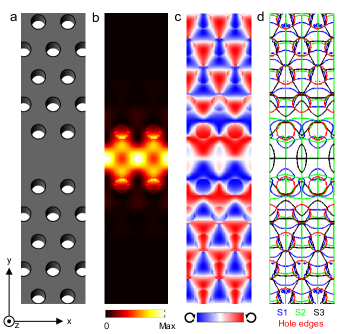
Figure 1: Polarisation of eigenmode of ideal waveguide. (a) Schematic of PhCWG, showing gallium arsenide membrane ($n=3.54$) etched with air holes. (b) Eigenmode of ideal waveguide $|E|^{2}$. (c) $S_{3}$, the extent to which the light is circularly polarised. (d) Zero-contours of the Stokes parameters $S_{1,2,3}$ shown by lines of the indicated shades. This figure, and all others in this paper, shows the fields at z=0 (centre of the slab).

In this work, we use calculations of the eigenmodes of disordered PhCWGs to demonstrate that the polarisation singularities (C-points and L-lines) present in the ideal waveguide persist far beyond realistically expected levels of disorder. By calculating the positions of these C-points and L-lines for a statistical ensemble of disordered waveguides, we demonstrate that not only do they persist, but their mean positions are close to those predicted for the ideal structure.

II Methods

Our PhCWG (shown in fig.1 (a)) is a single row of missing air holes from an hexagonal lattice of holes spaced $a$ apart and with a diameter of $d=0.48a$ in a dielectric slab with refractive index $n=3.54$ and thickness $h=0.56a$. The lattice constant $a$ can be chosen freely for different operating regimes, but with $a=250$ nm these values are suitable for a PhCWG in a GaAs membrane embedded with quantum dots emitting at 900 nm. We choose to work with a mode located at $ka/2\pi=0.35$ with a eigenfrequency of $\omega a/2\pi c=0.255$ and group velocity $v_{g}=c/7$. We chose this mode as it possesses a significant number of C-points in the vicinity of the waveguide core, making it well suited to collect statistics when disorder is introduced. Also the relatively modest slow-down factor ensures that the disorder localisation length remains longer than our waveguide supercell length, even for the largest disorder considered, ensuring that we remain in the ballistic photon transport regime and avoid complications caused by the formation of localised states in the disordered waveguides Mazoyer et al. (2010). The eigenmodes are calculated using a finite-difference time-domain (FDTD) method Oskooi. et al. (2010) with a grid resolution of $a/24$ and periodic boundary conditions in the direction of the waveguide (absorbing boundaries on all other edges). In the course of the simulation a large number of modes are excited by dipole sources placed in the waveguide, but letting the simulation evolve in time causes most of these modes to decay such that the remaining power is in the waveguide’s eigenmode $\mathbf{E}(\mathbf{r})$, as shown in fig.1 (b).

After finding the eigenmodes $\mathbf{E}(\mathbf{r})$, the polarisation structure in the vicinity of the waveguide is examined by calculating the four Stokes parameters, $S_{0,1,2,3}$, as a function of position $\mathbf{r}$. Together, the Stokes parameters completely specify the polarisation of the electric field on the Poincaré sphere Collett (2005):

$$S_{0}(\mathbf{r})=|E_{x}(\mathbf{r})|^{2}+|E_{y}(\mathbf{r})|^{2},$$ (1)

$$S_{1}(\mathbf{r})=(|E_{x}(\mathbf{r})|^{2}-|E_{y}(\mathbf{r})|^{2})/S_{0}(\mathbf{r}),$$

$$S_{2}(\mathbf{r})=2*Re(E_{x}^{*}(\mathbf{r})E_{y}(\mathbf{r}))/S_{0}(\mathbf{r}),$$

$$S_{3}(\mathbf{r})=2*Im(E_{x}^{*}(\mathbf{r})E_{y}(\mathbf{r}))/S_{0}(\mathbf{r}).$$

$S_{0}$ specifies the total electric field strength, $|\mathbf{E}|^{2}$, and $-1\leq S_{1,2,3}\leq 1$ are the positions on the Poincaré sphere. Figure 1 (b) shows the calculated value of $S_{0}$ in the central plane ($z=0$) of the membrane for the ideal photonic crystal waveguide, and Figure 1 (c) shows the value of $S_{3}$. $S_{3}$ is of particular interest to us, as it measures the extent of circular polarisation in the electric field profile. Positions where $S_{3}=\pm 1$ are C-points with fully left and right circularly polarised fields, whereas contours where $S_{3}=0$ are L-lines with linear polarisation. $S_{1}$ and $S_{2}$ indicate the degree of linear polarisation in the rectilinear and diagonal basis; specifically the values of $\pm 1$ in $S_{1}$ denotes vertical and horizontal polarization, while in $S_{2}$ they denote diagonal and anti-diagonal polarisation. Figure 1 (d) shows the contours of $S_{1,2,3}=0$ for our PhCWG, with blue, green and black lines respectively. The $S_{3}=0$ contour marks the L-lines, whereas the C-points are marked by the crossing of the $S_{1}=0$ and $S_{2}=0$ contours (so points where $S_{1}=S_{2}=0$) , which coincide with positions where $S_{3}=\pm 1$ (see Figure 2 (b)) Freund et al. (2002).

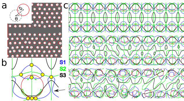
Figure 2: Effect of disorder on Stokes parameters. (a) Schematic of the disorder, the positions of the air holes in the ideal waveguide are shown in with lines, with a specific instance of a disordered crystal shaded in grey. Inset: the disorder model for an individual hole. (b) The zero-contours of $S_{1,2,3}$ are shown in blue, green and black respectively. The large circle denotes an air hole. C-points are marked with circles and L-lines by black lines. (c) More zero-contours (same colours), this time for supercells in three specific simulation runs with $\delta=$ 0, 0.03 and 0.09.

III Disorder Results

We now consider the effect of disorder on the Stokes parameters. All disorder and imperfections in the waveguide are modelled as a random shift in the positions of the holes, with each hole displaced a small distance selected from a normal distribution with a mean of zero and a standard deviation of $a\delta$ in a random direction $\theta$ (selected from a uniform distribution $0\leq\theta<\pi$). The parameter $\delta$ therefore characterises the level of disorder in the simulation. Although this model may not realistically represent all of the errors that occur in a typical fabrication process (it ignores the ellipticity, hole-size variation, side-wall roughness and angle), the displacement of the holes can be exaggerated in order to crudely account for these effects, and similar models of disorder are widely used Minkov et al. (2013); O’Faolain et al. (2007); Smolka et al. (2011); Moon and Yang (2013); Beggs et al. (2005). Each simulation of a disordered waveguide used a supercell of dimensions $15a$ x $24a$ x $5a$, containing 15 unit-cells along the direction of the waveguide. This length of 15 unit cells was chosen by checking that it is longer than the distance over which individual cells are significantly correlated with their neighbours whilst being significantly shorter than the disorder localisation length (see discussion in supplementary information). An example part of disordered supercell is illustrated in Figure 2 (a).

As described above, the position of the C-points are found in the eigenmodes of the disordered waveguides by examining where the zero contours of $S_{1}$ and $S_{2}$ cross, which is equivalent to finding positions where $S_{3}=\pm 1$. Figure 2 (b) shows the position of the C-points in one half of the unit cell of the ideal structure, in the vicinity of the hole closest to the waveguide. The contours of $S_{1,2,3}=0$ are shown by blue, green and black lines respectively, and the C-points are shown by the yellow dots. The L-lines are located simply by the contours where $S_{3}=0$ (black lines). Figure 2 (c) shows the response of the polarisation landscape to the introduction of disorder in the waveguide. The top panel shows the ideal case ($\delta=0$), the middle shows $\delta=0.03$ and the bottom $\delta=0.09$.

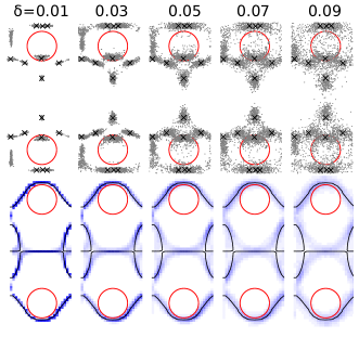
Figure 3: Top: the locations of C-points. Each panel shows all the C-points found for a particular choice of $\delta$ folded into a single unit cell (using data from 32 separate simulations). Crosses: locations of the C-points with no disorder. Bottom: probability density of L-lines. Black lines: locations of the L-lines with no disorder. The circles (in both sets of panels) show the positions of the air holes (without disorder).

The most obvious feature apparent in fig.2 (c) is that the zero-contours of the the Stokes parameters $S_{1,2,3}$ lose all sense of the symmetries present in the ideal structure. In particular, the L-lines ($S_{3}=0$) lose the crossings seen in the core of the ideal waveguide, even for small disorder. However, despite the apparent lack of order in fig.2 (c), a more through analysis reveals that the polarisation singularities are remarkably robust to disorder.

Although not shown by fig.2 (c) the number of points where the zero-contours of each Stokes parameter crosses itself falls rapidly with the introduction of disorder. Self crossings of this type imply the existence of two regions in which the Stokes parameter takes positive values and two where it takes negative ones meeting at a corner in a “chess board” like arrangement. In principle even the smallest amount of disorder will be sufficient to disturb this arrangement, creating a bridge connecting either the positive regions or the negative ones Freund and Shvartsman (1994); Nye (1983). We find that these points disappear extremely rapidly with the introduction of disorder, and believe that the surviving cases can be attributed to the finite resolution of the simulations.

Figure 3 shows a summary of the main findings of this work. The top row considers the C-points. Each panel in the top row marks with a blue dot the calculated positions of C-points found in each unit cell after 32 calculations performed with an independent realisation of the disordered structure for the values of the disorder parameter $\delta=$ 0.01, 0.03, 0.05, 0.07 and 0.09. The black crosses mark the positions of the C-points in the ideal structure. The bottom row considers the L-lines. Each panel in the bottom row shows the location of the L-lines in the same disordered waveguides. Specifically the probability of finding an L-line crossing a pixel in the calculation grid is plotted using a colour scale of white (zero probability) to dark blue (high probability) is shown. The L-lines in the ideal waveguide are shown by black lines.

Firstly, it is clear that the existence of polarisation singularities is largely robust to the addition of disorder. A few C-points are eliminated, but the majority survive in displaced locations (see below). For the smallest levels of disorder, the C-points and L-lines cluster very closely to their positions in the ordered waveguide, but they gradually move away with increasing disorder. For $\delta=0.01$, the C-points move a mean distance of just $0.06a$ away from their positions in the ideal case, and the L-line just $0.04a$, although these distances steadily increase with disorder, as shown in fig.4 (b).

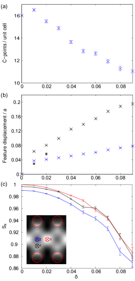
Figure 4: (a) The occurrence of C-points as a function of disorder. (b) Crosses (stars): mean distance of C-points (L-line vertices) in simulations of disordered structures from the nearest C-point (L-line) in a simulation of the ideal structure. Circles: mean displacement of C-points when newly created C-points are ignored. (c) The change in polarisation with disorder is plotted for three points, one of right circular polarisation (1) and two of transverse linear polarisation (2,3), for each the relevant Stokes parameter is plotted (3,1,1 respectively). Note that they do not begin at exactly 1; this is a result of finite resolution. The inset shows the locations of points 1,2 and 3 relative to the air holes.

As well as the elimination and displacement of C-points, the addition of disorder also causes their creation. Such C-points are apparent in fig.3, where clusters of C-points form that are not associated with any from the ideal waveguide (bottom- and top-left of each panel). In the ideal structure near these locations, there exist regions where the the ellipticity is high ($>0.9$), despite a C-point not being formed. The zero-contours of $S_{1}$ and $S_{2}$ come very close to crossing in the ideal waveguide (indicated by the arrow in fig.2 (b)), and when disorder is introduced, these contours move and can sometimes cross and thus form extra C-points. In fact, for the smallest levels of disorder considered ($\delta<0.02$), there are on average more C-points found in the disordered waveguides than in the ideal one. However, for $\delta>0.02$, the number of C-points found per unit cell falls slowly with increasing disorder, until for the highest levels of disorder considered, a mean of 11.1 $\pm 0.3$ from the original 16 per unit cell remain. Figure 4 (a) shows a plot of the mean number of C-points found per unit cell as a function of the disorder parameter $\delta$.

The creation of these new C-points increases the average separation between the C-points in disordered structures and those in the ideal structure. The two circles in fig.4 (b) show the mean displacement of C-points when the new C-points are excluded.

To further examine the effects of disorder on the polarisation singularities, we plot the mean values of the Stokes parameters at several key positions in the waveguide. These positions are at a C-point and on an L-line, and are shown in detail by the inset in fig.4 (c). The first point (labelled ”1”) is located at a C-point in the ideal structure, near the centre of the waveguide. Figure 4 (c) shows the mean value of $S_{3}$ averaged over all unit cells in all simulations as a function of the disorder parameter $\delta$ at this position. Being at a (right-handed) C-point means that the value in the ideal waveguide is $S_{3}=1$, but this reduces as disorder is introduced and the C-point is displaced or destroyed.

Also shown are two points (label ”2” and ”3”) that are both located on an L-line in the centre of the waveguide. Both these points have $S_{1}=1$ and $S_{3}=0$ in the ideal waveguide, and the mean value of $S_{1}$ averaged over the disordered structures are shown in fig.4 (c) as a function of $\delta$. Again, as disorder is introduced, the mean value of $S_{1}$ deceases, slowly at first, but then faster for higher disorders. The pattern is very similar to that of the value of the ellipticity $S_{3}$ at the C-point. Using the value of $S_{1}$ as a proxy for the ”amount of L-line-ness” at the points considered, it can thus be said that the L-lines and C-points display remarkably similar robustness to the introduction of disorder.

Taking fig.3 and 4 as a whole, we conclude that the existence of C-points and L-lines are remarkably robust to disorder in the waveguide, and that their positions in the disordered waveguides are on average very close to the positions in the ideal waveguide.

Our analysis so far has concentrated on the extremal points of polarisation (i.e. the C-points and L-lines). However, many applications may only require a large degree of polarisation to be viable. For example, while C-points with $S_{3}=\pm 1$ are strictly the only locations in the waveguide where a circular dipole will emit light in only one direction (unit directionality), regions possessing a high value of ellipticity $|S_{3}|$ will emit predominantly in one direction, as the directionality is equal to the ellipticity. Figure 4 (c) shows the decay of the ellipticity or directionality at the position of the C-point nearest to the centre of the waveguide, and from it we note that disorder parameters of $\delta\leq 0.085$ possess a mean directionality of greater than 90% at this position, and $\delta\leq 0.065$ a mean directionality of greater than 95%.

Figure 5 shows the regions where a circular dipole emitter embedded in the waveguide would possess a high directionality for a particular instance of a disordered waveguide; directionality above 0.9 in the lightly shaded regions and above 0.95 in the darker ones. It can be seen that moderate disorder ($\delta\leq 0.03$, middle panel) does not greatly impact these regions, but that very high disorder ($\delta=0.09$, bottom panel) has a large detrimental impact.

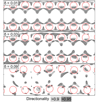
Figure 5: Regions of high directionality ($\equiv$ ellipticity) for three specific instances of disorder. Circles show the locations of the air holes.

IV Conclusion

We have shown that polarisation singularities in photonic crystal waveguides are remarkably robust to disorder in the waveguide, at least for this choice of mode. Using comparisons between experiment and calculations using a similar disorder model to ours in ref. Liu et al. (2014), we estimate that real photonic crystal waveguides display a level of disorder equivalent to $\delta=0.003$, more than 3 times smaller than the lowest disorder considered in this paper (note that the comparison used a InGaAsP photonic crystal with a hole spacing of $a=400$ nm for wavelengths around 1550 nm). Waveguide modes with smaller group velocities may be less robust than the mode studied here (with $v_{g}=c/7$), but our calculations suggest that even in the case of modes that are an order of magnitude more sensitive to disorder there will still be usable polarisation singularities. One proposal is to place a quantum dot at a C-point, where the electron spin will be coupled with the path information in the waveguide, useful in quantum information applications. For a quantum emitter placed at the C-point closest to the waveguide core, we find that the emission directionality is 99.6% $\pm$ 0.3% for a disorder of $\delta=0.01$. Given that site-control placement of quantum dots can be achieved with 50nm accuracy Schneider et al. (2008), our results indicate that a fabrication yield of 54% can be expected for emission directionality $>90$%, a number almost independent of the disorder parameter (for small $\delta$). For comparison of quantum dots grown randomly in the waveguide vicinity 21% can be expected to have an emission directionality $>90$% (dropping only to 20% for small $\delta$). The route to higher yields is to improve the quantum dot placement rather than the disorder in the PhCWG.

By outlining the tolerances to disorder, our results are an important step to realising spin-to-path behaviour in PhCWGs using current fabrication technologies.

See pages ,1,,2,,3,,4,,5,,6,,7 of supplement.pdf