Max-Cut under Graph Constraints

Abstract

An instance of the graph-constrained max-cut ($\mathsf{GCMC}$) problem consists of (i) an undirected graph $G=(V,E)$ and (ii) edge-weights $c:{V\choose 2}\rightarrow\mathbb{R}_{+}$ on a complete undirected graph. The objective is to find a subset $S\subseteq V$ of vertices satisfying some graph-based constraint in $G$ that maximizes the weight $\sum_{u\in S,v\not\in S}c_{uv}$ of edges in the cut $(S,V\setminus S)$. The types of graph constraints we can handle include independent set, vertex cover, dominating set and connectivity. Our main results are for the case when $G$ is a graph with bounded treewidth, where we obtain a $\frac{1}{2}$-approximation algorithm. Our algorithm uses an LP relaxation based on the Sherali-Adams hierarchy. It can handle any graph constraint for which there is a (certain type of) dynamic program that exactly optimizes linear objectives.

Using known decomposition results, these imply essentially the same approximation ratio for $\mathsf{GCMC}$ under constraints such as independent set, dominating set and connectivity on a planar graph $G$ (more generally for bounded-genus or excluded-minor graphs).

1 Introduction

The max-cut problem is an extensively studied combinatorial-optimization problem. Given an undirected edge-weighted graph, the goal is to find a subset $S\subseteq V$ of vertices that maximizes the weight of edges in the cut $(S,V\setminus S)$. Max-cut has a 0.878-approximation algorithm [14] which is known to be best-possible assuming the “unique games conjecture” [17]. It also has a number of practical applications, e.g., in circuit layout, statistical physics and clustering.

In some applications, one needs to solve the max-cut problem under additional constraints on the subset $S$. Consider for example, the following clustering problem. The input is an undirected graph $G=(V,E)$ representing, say, a social network (vertices $V$ denote users and edges $E$ denote connections between users), and a weight function $c:{V\choose 2}\rightarrow\mathbb{R}_{+}$ representing, a dissimilarity measure between pairs of users. The goal is to find a subset $S\subseteq V$ of users that are connected in $G$ while maximizing the weight of edges in the cut $(S,V\setminus S)$. This corresponds to finding a cluster of connected users that is as different as possible from its complement set. This “connected max-cut” problem also arises in image segmentation applications [22, 16].

Designing algorithms for constrained versions of max-cut is also interesting from a theoretical standpoint. For max-cut under certain types of constraints (such as cardinality or matroid constraints) good approximation algorithms are known, e.g., [2, 1]. In fact, many of these results have since been extended to the more general setting of submodular objectives [12, 9]. However, not much is known for max-cut under “graph-based” constraints as in the example above.

In this paper, we study a large class of graph-constrained max-cut problems and present unified approximation algorithms for them. Our results require that the constraint be defined on a graph $G$ of bounded treewidth. (Treewidth is a measure of how similar a graph is to a tree structure — see §2 for definitions.) We note however that for a number of constraints (including the connectivity example above), we can combine our algorithm with known decomposition results [10, 11] to obtain essentially the same approximation ratios when the constraint graph $G$ is planar/bounded-genus/excluded-minor.

Problem definition.

The input to the graph-constrained max-cut ($\mathsf{GCMC}$) problem consists of (i) an $n$-vertex undirected graph $G=(V,E)$ which implicitly specifies a collection ${\cal C}_{G}\subseteq 2^{V}$ of feasible vertex subsets, and (ii) (symmetric) edge-weights $c:{V\choose 2}\rightarrow\mathbb{R}_{+}$. The $\mathsf{GCMC}$ problem is then as follows:

$$\max_{S\in{\cal C}_{G}}\quad\sum_{u\in S,v\not\in S}c(u,v).$$ (1)

In this paper, we assume that the constraint graph $G$ has bounded treewidth. We also assume that the graph constraint ${\cal C}_{G}$ admits an exact dynamic program for optimizing a linear objective, i.e. for:

$$\max_{S\in{\cal C}_{G}}\quad\sum_{u\in S}f(u),\qquad\mbox{where $f:V\rightarrow\mathbb{R}$ is any given vertex weights}.$$ (2)

Note that the $\mathsf{GCMC}$ objective (1) is a quadratic function of the solution $S$, whereas our assumption (2) involves a linear function of the solution $S$. See §2 for more precise definitions/assumptions.

1.1 Our Results and Techniques

Our main result can be stated informally as follows.

Theorem 1.1 ($\mathsf{GCMC}$ result — informal)

Consider any instance of the $\mathsf{GCMC}$ problem on a bounded-treewidth graph $G=(V,E)$. Suppose there is an exact dynamic program for optimizing any linear function subject to constraint ${\cal C}_{G}$. Then we obtain a $\frac{1}{2}$-approximation algorithm for $\mathsf{GCMC}$.

This algorithm uses a linear-programming relaxation for $\mathsf{GCMC}$ based on the dynamic program (for linear objectives) which is further strengthened via the Sherali-Adams LP hierarchy. The resulting LP has polynomial size whenever the number of dynamic program states associated with a single tree-decomposition node is constant (see §2 for the formal definition). The rounding algorithm is a natural top-down procedure that randomly chooses a “state” for each tree-decomposition node using the LP’s probability distribution conditional on the choices at its ancestor nodes. The final solution is obtained by combining the chosen states at each tree-decomposition node, which is guaranteed to satisfy constraint ${\cal C}_{G}$ due to properties of the dynamic program. We note that the choice of variables in the Sherali-Adams LP as well as the rounding algorithm are similar to those used in [15] for the sparsest cut problem on bounded-treewidth graphs. An important difference in our result is that we apply the Sherali-Adams hierarchy to a non-standard LP that is defined using the dynamic program for linear objectives. (If we were to apply Sherali-Adams to the standard LP, then it is unclear how to enforce the constraint ${\cal C}_{G}$ during the rounding algorithm.) Another difference is that our rounding algorithm needs to make a correlated choice in selecting the states of sibling nodes in order to satisfy constraint ${\cal C}_{G}$— this causes the number of variables in the Sherali-Adams LP to increase, but it still remains polynomial since the tree-decomposition has constant degree.

The requirement in Theorem 1.1 on the graph constraint ${\cal C}_{G}$ is satisfied by several interesting constraints and thus we obtain approximation algorithms for all these $\mathsf{GCMC}$ problems. See Section 4 for details.

Theorem 1.2 (Applications)

There is a $\frac{1}{2}$-approximation algorithm for $\mathsf{GCMC}$ under the following constraints in a bounded-treewidth graph: independent set, vertex cover, dominating set, connectivity.

We note that many other constraints such as precedence, connected dominating set, and triangle matching also satisfy our requirement. In the interest of space, we only present details for the constraints mentioned in Theorem 1.2. We also note that for some of these constraints (e.g., independent set) one can come up with a problem specific algorithm where the approximation ratio depends on the treewidth $k$. Our result is stronger since the algorithm is more general, and the ratio is independent of $k$.

For many of the constraints above, we can use known decomposition results [10, 11] to obtain approximation algorithms for $\mathsf{GCMC}$ when the constraint graph has bounded genus or excludes some fixed minor (e.g., planar graphs).

Corollary 1

There is a $(\frac{1}{2}-\epsilon)$-approximation algorithm for $\mathsf{GCMC}$ under the following constraints in an excluded-minor graph: independent set, vertex cover, dominating set. Here $\epsilon>0$ is a fixed constant.

Corollary 2

There is a $(\frac{1}{2}-\epsilon)$-approximation algorithm for connected max-cut in a bounded-genus graph. Here $\epsilon>0$ is a fixed constant.

Our approach can also handle other types of objectives. If $g:2^{V}\rightarrow\mathbb{R}_{+}$ is the sum of a polynomial number of functions each of which is monotone, submodular and defined on a constant-size subset of $V$, then we obtain a $(1-\frac{1}{e})$-approximation algorithm for the problem of maximizing $g(S)$ subject to $S\in{\cal C}_{G}$. The graph constraint ${\cal C}_{G}$ is as above. The main idea is to use the correlation gap of monotone submodular function.[3, 9]

1.2 Related Work

For the basic undirected max-cut problem, there is an elegant 0.878-approximation algorithm [14] via semidefinite programming. This is also the best one can hope for, assuming the unique games conjecture [17].

Most of the prior work on constrained max-cut has focused on cardinality, matroid and knapsack constraints [2, 1, 12, 9, 18, 19]. Constant-factor approximation algorithms are known for max-cut under the intersection of any constant number of such constraints — these results hold in the substantially more general setting of non-negative submodular functions. The main techniques used here are local search and the multilinear extension [8] of submodular functions. These results made crucial use of certain exchange properties of the underlying constraints, which are not true for graph-based constraints that we consider.

Closer to our setting, a version of the connected max-cut problem was studied recently in [16], where the connectivity constraint as well as the weight function were defined on the same graph $G$. The authors obtained an $O(\log n)$-approximation algorithm for general graphs, and an exact algorithm on bounded-treewidth graphs (which implied a PTAS for bounded-genus graphs); their algorithms relied heavily on the uniformity of the constraint/weight graphs. In contrast, we consider the connected max-cut problem where the connectivity constraint and the weight function are unrelated; in particular, our problem generalizes max-cut even when $G$ is a trivial graph (e.g., a star). Moreover, our algorithms work for a much wider class of constraints. We note however that our results require graph $G$ to have bounded treewidth — this is also necessary since some of the constraints we consider (e.g., independent set) are inapproximable in general graphs. (For connected max-cut itself, obtaining a non-trivial approximation ratio when $G$ is a general graph remains an open question.)

In terms of techniques, the closest work to ours is [15]. We use ideas from [15] in formulating the (polynomial size) Sherali-Adams LP as well as in the rounding algorithm. There are important differences too, as discussed in §1.1.

Finally, our result adds to a somewhat small list [6, 20, 5, 4, 15, 13] of algorithmic results based on the Sherali-Adams [21] LP hierarchy. We are not aware of a more direct approach to obtain a constant-factor approximation algorithm even for connected max-cut when the constraint graph $G$ is a tree.

2 Preliminaries

Basic definitions. For an undirected complete graph on vertices $V$ and subset $S\subseteq V$, let $\delta S$ be the set of edges with exactly one end-point in $S$. For any weight function $c:{V\choose 2}\rightarrow\mathbb{R}_{+}$ and subset $F\subseteq{V\choose 2}$, we use $c(F):=\sum_{e\in F}c_{e}$.

Tree Decomposition. Given an undirected graph $G=(V,E)$, this consists of a tree ${\cal T}=(I,F)$ and a collection of vertex subsets $\{X_{i}\subseteq V\}_{i\in I}$ such that:

• for each $v\in V$, the nodes $\{i\in I:v\in X_{i}\}$ are connected in ${\cal T}$, and

• for each edge $(u,v)\in E$, there is some node $i\in I$ with $u,v\in X_{i}$.

The width of such a tree-decomposition is $\max_{i\in I}(|X_{i}|-1)$, and the treewidth of $G$ is the smallest width of any tree-decomposition for $G$.

We will work with “rooted” tree-decompositions that also specify a root node $r\in I$. The depth $d$ of such a tree-decomposition is the length of the longest root-leaf path in ${\cal T}$. The depth of any node $i\in I$ is the length of the $r-i$ path in ${\cal T}$.

For any $i\in I$, the set $V_{i}$ denotes all the vertices at or below node $i$, that is

$$V_{i}\quad:=\quad\cup_{k\in{\cal T}_{i}}\,\,X_{k},\quad\mbox{where }{\cal T}_{i}=\{k\in I:k\mbox{ in subtree of ${\cal T}$ rooted at }i\}.\vspace{-1mm}$$

The following known result provides a convenient representation of ${\cal T}$.

Theorem 2.1 (Balanced Tree Decomposition [7])

Let $G=(V,E)$ be a graph of treewidth $k$. Then $G$ has a rooted tree-decomposition $({\cal T}=(I,F),\{X_{i}|i\in I\})$ where ${\cal T}$ is a binary tree of depth $2\lceil\log_{\frac{5}{4}}(2|V|)\rceil$ and treewidth at most $3k+2$. This tree-decomposition can be found in $O(|V|)$ time.

Dynamic program for linear objectives.

We assume that the constraint ${\cal C}_{G}$ admits an exact dynamic programming (DP) algorithm for optimizing linear objectives, i.e. for the problem (2). There is some additional notation that is needed to formally describe the DP: this is necessary due to the generality of our results.

Definition 1 (DP)

With any tree-decomposition $({\cal T}=(I,F),\{X_{i}|i\in I\})$, we associate the following:

1. For each node $i\in I$, there is a state space $\Sigma_{i}$.

2. For each node $i\in I$ and $\sigma\in\Sigma_{i}$, there is a collection ${\cal H}_{i,\sigma}\subseteq 2^{V_{i}}$ of subsets.

3. For each node $i\in I$, its children nodes $\{j,j^{\prime}\}$ and $\sigma\in\Sigma_{i}$, there is a collection ${\cal F}_{i,\sigma}\subseteq\Sigma_{j}\times\Sigma_{j^{\prime}}$ of valid combinations of children states.

Assumption 1 (Linear objective DP for ${\cal C}_{G}$)

Let $({\cal T}=(I,F),\{X_{i}|i\in I\})$ be any tree-decomposition. Then there exist $\Sigma_{i}$, ${\cal F}_{i,\sigma}$ and ${\cal H}_{i,\sigma}$ (see Definition 1) that satisfy the following:

1. (bounded state space) $\Sigma_{i}$ and ${\cal F}_{i,\sigma}$ are all bounded by constant, that is, $\max_{i}{|\Sigma_{i}|}=t$ and $\max_{i,\sigma}{|{\cal F}_{i,\sigma}|}=p$, where $t,p=O(1)$.

2. (required state) For each $i\in I$ and $\sigma\in\Sigma_{i}$, the intersection with $X_{i}$ of every set in ${\cal H}_{i,\sigma}$ is the same, denoted $X_{i,\sigma}$, that is $S\cap X_{i}=X_{i,\sigma}$ for all $S\in{\cal H}_{i,\sigma}$.

3. (subproblem) For each non-leaf node $i\in I$ with children $\{j,j^{\prime}\}$ and $\sigma\in\Sigma_{i}$,

   $${\cal H}_{i,\sigma}\quad=\quad\left\{X_{i,\sigma}\cup S_{j}\cup S_{j^{\prime}}\,\,:\,\,S_{j}\in{\cal H}_{j,w_{j}},\,S_{j^{\prime}}\in{\cal H}_{j^{\prime},w_{j^{\prime}}},\,(w_{j},w_{j^{\prime}})\in{\cal F}_{i,\sigma}\right\}.$$

   By condition 2, for any leaf $\ell\in I$ and $\sigma\in\Sigma_{\ell}$, we have ${\cal H}_{\ell,\sigma}=\{X_{\ell,\sigma}\}$ or $\emptyset$.

4. (cover all constraints) At the root node $r$, we have ${\cal C}_{G}=\bigcup_{\sigma\in\Sigma_{r}}{{\cal H}_{r,\sigma}}$.

The most restrictive assumption is the first condition. To the best of our knowledge, all natural constraints that admit a dynamic program on bounded-treewidth graphs (for linear objectives) satisfy conditions 2-4. Even in cases when condition 1 is not true, a relaxed version holds (where $t$ and $p$ are polynomial), and our approach gives a quasi-polynomial time $\frac{1}{2}$-approximation algorithm.

Example:

Here we outline how independent set satisfies the above requirements.

• The state space of each node $i\in I$ consists of all independent subsets of $X_{i}$.

• The subsets ${\cal H}_{i,\sigma}$ consist of all independent subsets $S\subseteq V_{i}$ with $S\cap X_{i}=\sigma$.

• The valid combinations ${\cal F}_{i,\sigma}$ consist of all tuples $(w_{j},w_{j^{\prime}})$ where the child states $w_{j}$ and $w_{j^{\prime}}$ are “consistent” with state $\sigma$ at node $i$.

A formal proof of why the independent-set constraint satisfies Assumption 1 appears in Section 4. There, we also discuss a number of other graph constraints satisfying our assumption.

The following result follows from Assumption 1.

Claim 1

For any $S\in{\cal C}_{G}$, there is a collection $\{b(i)\in\Sigma_{i}\}_{i\in I}$ such that:

• for each node $i\in I$ with children $j$ and $j^{\prime}$, $(b(j),b(j^{\prime}))\in{\cal F}_{i,b(i)}$,

• for each leaf $\ell$ we have ${\cal H}_{\ell,b(\ell)}\neq\emptyset$, and

• $S=\bigcup_{i\in I}X_{i,b(i)}$.

Moreover, for any vertex $u\in V$, if $\overline{u}\in I$ denotes the highest node containing $u$ then $u\in S\iff u\in X_{\overline{u},b(\overline{u})}$.

Proof

We define the states $b(i)$ in a top-down manner; we will also define an associated subset $B_{i}\in{\cal H}_{i,b(i)}$ at each node $i$. At the root, we set $b(r)=\sigma$ such that $S\in{\cal H}_{r,\sigma}$: this is well-defined by Assumption 1(4). We also set $B_{r}=S$. Having set $b(i)$ and $B_{i}\in{\cal H}_{i,b(i)}$ for any node $i\in I$ with children $\{j,j^{\prime}\}$, we use Assumption 1(3) to write

$$B_{i}=X_{i,b(i)}\cup S_{j}\cup S_{j^{\prime}}\quad\mbox{where }S_{j}\in{\cal H}_{j,w_{j}},\,S_{j^{\prime}}\in{\cal H}_{j^{\prime},w_{j^{\prime}}}\mbox{ and }(w_{j},w_{j^{\prime}})\in{\cal F}_{i,b(i)}.$$

Then we set $b(j)=w_{j}$ and $B_{j}=S_{j}$ for all the children $J$ of node $i$. It is now easy to verify the first three conditions in the claim.

Since $S=\bigcup_{i\in I}X_{i,b(i)}$, it is clear that $u\in X_{\overline{u},b(\overline{u})}\implies u\in S$. In the other direction, suppose $u\not\in X_{\overline{u},b(\overline{u})}$: we will show $u\not\in S$. Since $\overline{u}$ is the highest node containing $u$, it suffices to show that $u\not\in B_{\overline{u}}$ above. But this follows directly from Assumption 1(2) since $B_{\overline{u}}\in{\cal H}_{\overline{u},b(\overline{u})}$, $u\in X_{\overline{u}}$ and $u\not\in X_{\overline{u},b(\overline{u})}$.  

Sherali-Adams LP hierarchy.

This is one of the several “lift-and-project” procedures that, given a $\{0,1\}$ integer program, produces systematically a sequence of increasingly tighter convex relaxations. The Sherali-Adams procedure [21] involves generating stronger LP relaxations by adding new variables and constraints. The $r^{th}$ round of this procedure has a variable $y(S)$ for every subset $S$ of at most $r$ variables in the original integer program — the new variable $y(S)$ corresponds to the joint event that all the original variables in $S$ are one.

3 Approximation Algorithm for $\mathsf{GCMC}$

In this section, we prove:

Theorem 3.1

Consider any instance of the $\mathsf{GCMC}$ problem on a bounded-treewidth graph $G=(V,E)$. If the graph constraint ${\cal C}_{G}$ satisfies Assumption 1 then we obtain a

$\frac{1}{2}$-approximation algorithm.

Algorithm outline:

We start with a balanced tree-decomposition ${\cal T}$ of graph $G$, as given in Theorem 2.1; recall the associated definitions from §2. Then we formulate an LP relaxation of the problem using Assumption 1 (i.e. the dynamic program for linear objectives) and further strengthened by applying the Sherali-Adams operator. Finally we use a natural top-down rounding that relies on Assumption 1 and the Sherali-Adams constraints.

3.1 Linear Program

We start with some additional notation related to the tree-decomposition ${\cal T}$ (from Theorem 2.1) and our dynamic program assumption (Assumption 1).

• For any node $i\in I$, $T_{i}$ is the set of nodes on the $r-i$ path along with the children of all nodes except $i$ on this path. See also Figure 1.

• ${\cal P}$ is the collection of all node subsets $J$ such that $J\subseteq T_{\ell_{1}}\cup T_{\ell_{2}}$ for some pair of leaf-nodes $\ell_{1},\ell_{2}$. See also Figure 1.

• $s(i)\in\Sigma_{i}$ denotes a state at node $i$. Moreover, for any subset of nodes $N\subseteq I$, we use the shorthand $s(N):=\{s(k):k\in N\}$.

• $\bar{u}\in I$ denotes the highest tree-decomposition node containing vertex $u$.

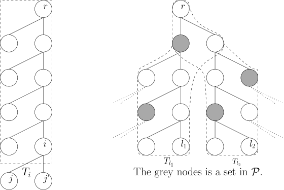
Figure 1: Examples of (i) a set $T_{i}$ and (ii) a set in ${\cal P}$.

The variables in our LP are $y(s(N))$ for all $\{s(k)\in\Sigma_{k}\}_{k\in N}$ and $N\in{\cal P}$. Variable $y(s(N))$ corresponds to the joint event that the solution (in ${\cal C}_{G}$) “induces” state $s(k)$ (in terms of Assumption 1) at each node $k\in N$.

We also use variables $z_{uv}$ defined in constraint (3) that measure the probability of an edge $(u,v)$ being cut. Constraints (4) are the Sherali-Adams constraints that enforce consistency among the $y$ variables. Constraints (5)-(7) are from the dynamic program (Assumption 1) and require valid state selections.

$$\mbox{maximize }\sum_{\{u,v\}\in{V\choose 2}}{c_{uv}z_{uv}}$$ (LP)

$$z_{uv}\,\,=\,\,\sum_{\begin{subarray}{c}s(\bar{u})\in\Sigma_{\bar{u}}\\ u\in X_{\bar{u},s(\bar{u})}\end{subarray}}\sum_{\begin{subarray}{c}s(\bar{v})\in\Sigma_{\bar{v}}\\ v\not\in X_{\bar{v},s(\bar{v})}\end{subarray}}{y(s(\{\bar{u},\bar{v}\}))}+\sum_{\begin{subarray}{c}s(\bar{u})\in\Sigma_{\bar{u}}\\ u\not\in X_{\bar{u},s(\bar{u})}\end{subarray}}\sum_{\begin{subarray}{c}s(\bar{v})\in\Sigma_{\bar{v}}\\ v\in X_{\bar{v},s(\bar{v})}\end{subarray}}{y(s(\{\bar{u},\bar{v}\}))},$$

$$\qquad\qquad\qquad\qquad\qquad\qquad\qquad\qquad\qquad\qquad\qquad\qquad\forall\{u,v\}\in{V\choose 2};$$ (3)

$$y(s(N))\,\,=\,\,\sum_{s(i)\in\Sigma_{i}}{y(s(N\cup\{i\}))},\qquad\forall N\in{\cal P},\,i\notin N\,:\,N\cup\{i\}\in{\cal P};$$ (4)

$$\sum_{s(r)\in\Sigma_{r}}y(s(r))=1;$$ (5)

$$y(s(\{i,j,j^{\prime}\}))\,=\,0,\qquad\qquad\quad\forall i\in I,\,s(i)\in\Sigma_{i},\,(s(j),s(j^{\prime}))\notin{\cal F}_{i,s(i)};$$ (6)

$$y(s(\ell))\,=\,0,\qquad\qquad\qquad\qquad\qquad\quad\,\,\,\forall\ell\in I,s(\ell)\in\Sigma_{\ell}:{\cal H}_{\ell,s(\ell)}=\emptyset;$$ (7)

$$0\,\,\leq\,\,y(s(N))\,\,\leq\,\,1,\qquad\qquad\qquad\qquad\qquad\forall N\in{\cal P},\,\{s(k)\in\Sigma_{k}\}_{k\in N}.$$ (8)

Claim 2

For any node $i\in I$ with children $j,j^{\prime}$ and $s(k)\in\Sigma_{k}$ for all $k\in T_{i}$,

$$y(s(T_{i}))\,\,=\,\,\sum_{s(j)\in\Sigma_{j}}\,\,\sum_{s(j^{\prime})\in\Sigma_{j^{\prime}}}{y(s(T_{i}\cup\{j,j^{\prime}\})}.$$ (9)

Proof

Note that $T_{i}\cup\{j,j^{\prime}\}\subseteq T_{\ell}$ for any leaf node $\ell$ in the subtree below $i$. So $T_{i}\cup\{j,j^{\prime}\}\in{\cal P}$ and the variables $y(s(T_{i}\cup\{j,j^{\prime}\})$ are well-defined. The claim now follows by two applications of constraint (4).  

In constraint (6), we use $j$ and $j^{\prime}$ to denote the two children of node $i\in I$.

3.2 The Rounding Algorithm

We start with the root node $r\in I$. Here $\{y(s(r))\,:\,s(r)\in\Sigma_{r}\}$ defines a probability distribution over the states of $r$. We sample a state $a(r)\in\Sigma_{r}$ from this distribution. Then we continue top-down: given the chosen state $a(i)$ of any node $i$, we sample states for both children of $i$ simultaneously from their joint distribution given at node $i$.

Input : Optimal solution of LP.

Output : A vertex set in ${\cal C}_{G}$.

1 Sample a state $a(r)$ at the root node by distribution $y(s(r))$;

2 Do process all nodes $i$ in ${\cal T}$ in order of increasing depth :

3       Sample states $a(j),a(j^{\prime})$ for the children of node $i$ by joint distribution

$$\Pr[a(j)=s(j)\mbox{ and }a(j^{\prime})=s(j^{\prime})]\,\,=\,\,\frac{y(s(T_{i}\cup\{j,j^{\prime}\}))}{y(s(T_{i}))},$$ (10)

where $s(T_{i})=a(T_{i})$.

4 end

5Do process all nodes $i$ in ${\cal T}$ in order of decreasing depth :

6       $R_{i}=X_{i,a(i)}\cup R_{j}\cup R_{j^{\prime}}$ where $j,j^{\prime}$ are the children of $i$.

7 end

8$R=R_{r}$;

return $R$.

Algorithm 1 Rounding Algorithm for LP

3.3 Algorithm Analysis

Lemma 1

(LP) is a valid relaxation of $\mathsf{GCMC}$.

Proof

Let $S\in{\cal C}_{G}$ be any feasible solution to the $\mathsf{GCMC}$ instance. Let $\{b(i)\}_{i\in I}$ denote the states given by Claim 1 corresponding to $S$. For any subset $N\in{\cal P}$ of nodes, and for all $\{s(i)\in\Sigma_{i}\}_{i\in N}$, set

$$y(s(N))=\left\{\begin{array}[]{ll}1,&\mbox{ if $s(i)=b(i)$ for all }i\in N;\\ 0,&\mbox{ otherwise.}\end{array}\right.$$

It is easy to see that constraints (4) and (8) are satisfied. By the first two properties in Claim 1, it follows that constraints (6) and (7) are also satisfied. The last property in Claim 1 implies that $u\in S\iff u\in X_{\overline{u},b(\overline{u})}$ for any vertex $u\in V$. So any edge $\{u,v\}$ is cut exactly when one of the following occurs:

• $u\in X_{\overline{u},b(\overline{u})}$ and $v\not\in X_{\overline{v},b(\overline{v})}$;

• $u\not\in X_{\overline{u},b(\overline{u})}$ and $v\in X_{\overline{v},b(\overline{v})}$.

Using the setting of variable $z_{uv}$ in (3) it follows that $z_{uv}$ is exactly the indicator of edge $\{u,v\}$ being cut by $S$. Thus the objective value in  (LP) is $c(\delta S)$.  

Lemma 2

(LP) has a polynomial number of variables and constraints. Hence the overall algorithm runs in polynomial time.

Proof

There are ${n\choose 2}=O(n^{2})$ variables $z_{uv}$. Since the tree is binary, we have $|T_{i}|\leq 2d$ for any node $i$, where $d=O(\log n)$ is the depth of the tree-decomposition. Moreover there are only $O(n^{2})$ pairs of leaves as there are $O(n)$ leaf nodes. For each pair $\ell_{1},\ell_{2}$ of leaves, we have $|T_{\ell_{1}}\cup T_{\ell_{2}}|\leq 4d$. Thus $|{\cal P}|\leq O(n^{2})\cdot 2^{4d}=poly(n)$. By Assumption 1, we have $\max|{\cal H}_{i,\sigma}|=t=O(1)$, so the number of $y$-variables is at most $|{\cal P}|\cdot t^{4d}=poly(n)$. This shows that  (LP) has polynomial size and can be solved optimally in polynomial time. Finally, it is easy to see that the rounding algorithm runs in polynomial time.  

Lemma 3

The algorithm’s solution $R$ is always feasible.

Proof

Note that the distribution used in Step 1 is always valid due to Claim 2; so the states $a(i)$s are well-defined.

We now show that for any node $i\in I$ with children $j,j^{\prime}$ we have $(a(j),a(j^{\prime}))\in{\cal F}_{i,a(i)}$. Indeed, at the iteration for node $i$ (when $a(j)$ and $a(j^{\prime})$ are set) using the probability distribution in (10) and by constraint (6), we obtain that $(a(j),a(j^{\prime}))\in{\cal F}_{i,a(i)}$ with probability one.

We show that for each node $i\in I$, the subset $R_{i}\in{\cal H}_{i,a(i)}$ by induction on the height of $i$. The base case is when $i$ is a leaf. In this case, due to constraint (7) (and the validity of the rounding algorithm) we know that ${\cal H}_{i,a(i)}\neq\emptyset$. So $R_{i}=X_{i,a(i)}\in{\cal H}_{i,a(i)}$ by Assumption 1(3). For the inductive step, consider node $i\in I$ with children $j,j^{\prime}$ where $R_{j}\in{\cal H}_{j,a(j)}$ and $R_{j^{\prime}}\in{\cal H}_{j^{\prime},a(j^{\prime})}$. Moreover, from the property above, $(a(j),a(j^{\prime}))\in{\cal F}_{i,a(i)}$. Now using Assumption 1(3) we have $R_{i}=X_{i,a(i)}\cup R_{j}\cup R_{j^{\prime}}\in{\cal H}_{i,a(i)}$. Thus the final solution $R\in{\cal C}_{G}$.  

Claim 3

A vertex $u$ is contained in solution $R$ if and only if $u\in X_{\bar{u},a(\bar{u})}$.

Proof

This proof is identical to that of the last property in Claim 1.  

In the rest of this section, we show that every edge $(u,v)$ is cut by solution $R$ with probability at least $z_{uv}/2$, which would prove the algorithm’s approximation ratio. Lemma 4 handles the case when $\bar{u}\in T_{\bar{v}}$ (the case $\bar{v}\in T_{\bar{u}}$ is identical). And Lemma 5 handles the (harder) case when $\bar{u}\not\in T_{\bar{v}}$ and $\bar{v}\not\in T_{\bar{u}}$.

We first state some useful claims before proving the lemmas.

Observation 1 (see [15] for a similar use of this principle)

Let $X,Y$ be two jointly distributed $\{0,1\}$ random variables. Then $\Pr(X=1)\Pr(Y=0)+\Pr(X=0)\Pr(Y=1)\geq\frac{1}{2}[\Pr(X=0,Y=1)+\Pr(X=1,Y=0)]$.

Proof

Let $\Pr(X=0,Y=0)=x$, $\Pr(X=0)=a$, $\Pr(Y=0)=b$. The probability table is as below:

$\quad x\quad$	$a-x$	$a$
$\quad b-x\quad$	$\quad 1+x-a-b\quad$	$1-a$
$b$	$1-b$

Then we want to show $a(1-b)+b(1-a)\geq\frac{1}{2}(a+b-2x)\Leftrightarrow a+b+2x\geq 4ab$. Since each probability is in $[0,1]$, we have $0\leq x\leq\min\{a,b\}$ and $a+b-1\leq x$.

If $a+b>1$, we have $a+b+2x\geq 3a+3b-2>1$. If $ab<\frac{1}{4}$, it is done. If $\frac{1}{4}\leq ab\leq 1$, we have $6\sqrt{ab}-2\geq 4ab$. Then $a+b+2x\geq 3a+3b-2\geq 4ab$.

If $a+b\leq 1$, we have $a+b+2x\geq a+b\geq 2\sqrt{ab}\geq 4ab$.

Combine the above two cases, we have the observation is true.  

Claim 4

For any node $i$ and state $s(k)\in\Sigma_{k}$ for all $k\in T_{i}$, the rounding algorithm satisfies $\Pr[a(T_{i})=s(T_{i})]=y(s(T_{i}))$.

Proof

We proceed by induction on the depth of node $i$. It is clearly true when $i=r$, i.e. $T_{i}=\{r\}$. Assuming the statement is true for node $i$, we will prove it for $i$’s children. Let $j,j^{\prime}$ be the children nodes of $i$; note that $T_{j}=T_{j^{\prime}}=T_{i}\cup\{j,j^{\prime}\}$. Then using (10), we have

$$\Pr[a(T_{j})=s(T_{j})\,\,|\,\,a(T_{i})=s(T_{i})]\quad=\quad\frac{y(s(T_{i}\cup\{j,j^{\prime}\}))}{y(s(T_{i}))}.$$

Combined with $\Pr[a(T_{i})=s(T_{i})]=y(s(T_{i}))$ we obtain $\Pr[a(T_{j})=s(T_{j})]=y(s(T_{j}))$ as desired.  

Claim 5

For any $u,v\in V$, $s(\bar{u})\in\Sigma_{\bar{u}}$ and $s(\bar{v})\in\Sigma_{\bar{v}}$, we have

$$y(s(\{\bar{u},\bar{v}\}))=\sum_{\begin{subarray}{c}s(k)\in\Sigma_{k}\\ k\in T_{i}\setminus\bar{u}\setminus\bar{v}\end{subarray}}y(s(T_{i}\cup\{\bar{u},\bar{v}\})),$$

where $i$ is the least common ancestor of $\bar{u}$ and $\bar{v}$.

Proof

Since $i$ is the least common ancestor of $\bar{u}$ and $\bar{v}$, we have $T_{i}\cup\{\bar{u},\bar{v}\}\in{\cal P}$. Then the claim follows by repeatedly applying constraint (4).  

Lemma 4

Consider any $u,v\in V$ such that $\bar{u}\in T_{\bar{v}}$. Then the probability that edge $(u,v)$ is cut by solution $R$ is $z_{uv}$.

Proof

Applying Claim 4 with node $i=\bar{v}$, for any $\{s(k)\in\Sigma_{k}:k\in T_{\bar{v}}\}$, we have $\Pr[a(T_{\bar{v}})=s(T_{\bar{u}})]=y(s(T_{\bar{u}}))$. Let $D_{u}=\{s(\bar{u})\in\Sigma_{\bar{u}}|u\in s(\bar{u})\}$ and $D_{v}=\{s(\bar{v})\in\Sigma_{\bar{v}}|v\in s(\bar{v})\}$. Since $\bar{u}\in T_{\bar{v}}$,

$$\Pr[u\in R,v\not\in R]=\sum_{s(\bar{u})\in D_{u}}\sum_{s(\bar{v})\not\in D_{v}}\sum_{\begin{subarray}{c}s(k)\in\Sigma_{k}\\ k\in T_{\bar{v}}\setminus\bar{u}\setminus\bar{v}\end{subarray}}y(s(T_{\bar{u}}))=\sum_{s(\bar{u})\in D_{u}}\sum_{s(\bar{v})\not\in D_{v}}y(s(\bar{u},\bar{v}))$$

The last equality above is by repeated application of constraint (4). Similarly we have

$$\Pr[u\not\in R,v\in R]=\sum_{s(\bar{u})\not\in D_{u}}\sum_{s(\bar{v})\in D_{v}}y(s(\bar{u},\bar{v})),$$

which combined with constraint (5) implies $\Pr[|\{u,v\}\cap R|=1]=z_{uv}$.  

Lemma 5

Consider any $u,v\in V$ such that $\bar{u}\not\in T_{\bar{v}}$ and $\bar{v}\not\in T_{\bar{u}}$. Then the probability that edge $(u,v)$ is cut by solution $R$ is at least $z_{uv}/2$.

Proof

In order to simplify notation, we define:

$$z^{+}_{uv}\,\,=\,\,\sum_{\begin{subarray}{c}s(\bar{u})\in\Sigma_{\bar{u}}\\ u\in X_{\bar{u},s(\bar{u})}\end{subarray}}\sum_{\begin{subarray}{c}s(\bar{v})\in\Sigma_{\bar{v}}\\ v\not\in X_{\bar{v},s(\bar{v})}\end{subarray}}{y(s(\{\bar{u},\bar{v}\}))},\quad z^{-}_{uv}\,\,=\,\,\ \sum_{\begin{subarray}{c}s(\bar{u})\in\Sigma_{\bar{u}}\\ u\not\in X_{\bar{u},s(\bar{u})}\end{subarray}}\sum_{\begin{subarray}{c}s(\bar{v})\in\Sigma_{\bar{v}}\\ v\in X_{\bar{v},s(\bar{v})}\end{subarray}}{y(s(\{\bar{u},\bar{v}\}))}.$$

Note that $z_{uv}=z_{uv}^{+}+z_{uv}^{-}$.

Let $D_{u}=\{s(\bar{u})\in\Sigma_{\bar{u}}|u\in s(\bar{u})\}$ and $D_{v}=\{s(\bar{v})\in\Sigma_{\bar{v}}|v\in s(\bar{v})\}$. Let $i$ denote the least common ancestor of nodes $\bar{u}$ and $\bar{v}$. For any choice of states $\{s(k)\in\Sigma_{k}\}_{k\in T_{i}}$ define:

$$z^{+}_{uv}(s(T_{i}))=\sum_{s(\bar{u})\in D_{u}}\sum_{s(\bar{v})\not\in D_{v}}\frac{y(s(T_{i}\cup\{\bar{u},\bar{v}\}))}{y(s(T_{i}))},$$

and similarly $z^{-}_{uv}(s(T_{i}))$.

In the rest of the proof we fix states $\{s(k)\in\Sigma_{k}\}_{k\in T_{i}}$ and condition on the event ${\cal E}$ that $a(T_{i})=s(T_{i})$. We will show:

$$\Pr[|\{u,v\}\cap R|=1\,|\,{\cal E}]\,\,\geq\,\,\frac{1}{2}\left(z^{+}_{uv}(s(T_{i}))+z^{-}_{uv}(s(T_{i}))\right).$$ (11)

By taking expectation over the conditioning $s(T_{i})$, this would imply Lemma 5.

We now define the following indicator random variables (conditioned on ${\cal E}$).

$$I_{u}=\begin{cases}0\quad\mbox{ if }a(\bar{u})\not\in D_{u}\\ 1\quad\mbox{ if }a(\bar{u})\in D_{u}\end{cases}\quad\mbox{and}\quad I_{v}=\begin{cases}0\quad\mbox{ if }a(\bar{v})\not\in D_{v}\\ 1\quad\mbox{ if }a(\bar{v})\in D_{v}\end{cases}.$$

Observe that $I_{u}$ and $I_{v}$ (conditioned on ${\cal E}$) are independent since $\bar{u}\not\in T_{\bar{v}}$ and $\bar{v}\not\in T_{\bar{u}}$. So,

$$\Pr[|\{u,v\}\cap R|=1\,|\,{\cal E}]\,\,=\,\,\Pr[I_{u}=1]\cdot\Pr[I_{v}=0]+\Pr[I_{u}=0]\cdot\Pr[I_{v}=1]$$ (12)

For any $s(k)\in\Sigma_{k}$ for $k\in T_{\bar{u}}\setminus T_{i}$, we have by Claim 4 and $T_{i}\subseteq T_{\bar{u}}$ that

$$\Pr[a(T_{\bar{u}})=s(T_{\bar{u}})\,|\,a(T_{i})=s(T_{i})]=\frac{\Pr[a(T_{\bar{u}})=s(T_{\bar{u}})]}{\Pr[a(T_{i})=s(T_{i})]}=\frac{y(s(T_{\bar{u}}))}{y(s(T_{i}))}.$$

Therefore

$$\Pr[I_{u}=1]\,\,=\,\,\sum_{s(\bar{u})\in D_{u}}\,\,\sum_{\begin{subarray}{c}k\in T_{\bar{u}}\setminus T_{i}\setminus\{\bar{u}\}\\ s(k)\in\Sigma_{k}\end{subarray}}\frac{y(s(T_{\bar{u}}))}{y(s(T_{i}))}=\sum_{s(\bar{u})\in D_{u}}\frac{y(s(T_{i}\cup\{\bar{u}\}))}{y(s(T_{i}))}.$$

The last equality follows from the (4) constraint. Similarly,

$$\Pr[I_{v}=1]\,\,=\,\,\sum_{s(\bar{v})\in D_{v}}\frac{y(s(T_{i}\cup\{\bar{v}\}))}{y(s(T_{i}))}.$$

Now define $\{0,1\}$ random variables $X$ and $Y$ jointly distributed as:

$$\begin{array}[]{|c|c|c|}\hline\cr&Y=0&Y=1\\ \hline\cr X=0&\Pr[I_{v}=1]-z_{uv}^{-}(s(T_{i}))&z_{uv}^{-}(s(T_{i}))\\ \hline\cr X=1&z_{uv}^{+}(s(T_{i}))&\Pr[I_{u}=1]-z_{uv}^{+}(s(T_{i}))\\ \hline\cr\end{array}$$

Note that $\Pr[X=1]=\Pr[I_{u}=1]$ and $\Pr[Y=1]=\Pr[I_{v}=1]$. So, applying Observation 1 and using (12) we have:

$$\Pr[|\{u,v\}\cap R|=1\,|\,{\cal E}]\,\,\geq\,\,\frac{1}{2}\left(\Pr[X=0,Y=1]+\Pr[X=1,Y=0]\right),$$

which implies (11).  

4 Applications

In this section, we show a number of graph constraints that satisfy Assumption 1 and thereby obtain $\frac{1}{2}$-approximation algorithms for $\mathsf{GCMC}$ under these constraints (on bounded-treewidth graphs).

Recall that the underlying graph $G$ is given by its tree-decomposition $({\cal T}=(I,F),\{X_{i}|i\in I\})$ from Theorem 2.1. Recall also the definition of a dynamic program on this tree-decomposition, as given in Definition 1.

4.1 Independent Set

Given graph $G=(V,E)$ and edge-weights $c:{V\choose 2}\rightarrow\mathbb{R}_{+}$ we want to maximize $c(\delta S)$ where $S$ is an independent set in $G$.

For each node $i\in I$ define state space $\Sigma_{i}=\{\sigma\subseteq X_{i}\,|\,\sigma\mbox{ is an independent set}\}$. For each node $i\in I$ and $\sigma\in\Sigma_{i}$, we define:

• set $X_{i,\sigma}=\sigma$.

• collection ${\cal H}_{i,\sigma}=\{S\subseteq V_{i}\,|\,X_{i}\cap S=\sigma\mbox{ and $S$ is an independent set in }G[V_{i}]\}$.

• ${\cal F}_{i,\sigma}=\{(w_{j_{1}},w_{j_{2}})\,|\,\mbox{for each }j\in\{j_{1},j_{2}\},\,w_{j}\in\Sigma_{j}\mbox{ such that }w_{j}\cap X_{i}=\sigma\cap X_{j}\}$ which denotes valid combinations. Note that the condition $w_{j}\cap X_{i}=\sigma\cap X_{j}$ enforces $w_{j}$ to agree with $\sigma$ on vertices of $X_{i}\cap X_{j}$.

We next show that these satisfy all the conditions in Assumption 1.

Assumption 1 part 1. We have $t=\max{|\Sigma_{i}|}\leq 2^{k}=O(1)$ for bounded-treewidth $k$. Also $p=\max{|{\cal F}_{i,\sigma}|}\leq t^{2}$ since each node has at most two children.

Assumption 1 part 2. By definition, for any $S\in{\cal H}_{i,\sigma}$ we have $S\cap X_{i}=\sigma=X_{i,\sigma}$.

Assumption 1 part 3. For any leaf $\ell\in I$ and $\sigma\in\Sigma_{\ell}$ it is clear that ${\cal H}_{\ell,\sigma}=\{X_{i,\sigma}\}$.

Consider now any non-leaf node $i$ and $\sigma\in\Sigma_{i}$. Let

$${\cal Z}\,\,=\,\,\{X_{i,\sigma}\cup S_{j_{1}}\cup S_{j_{2}}\,:\,S_{j_{1}}\in{\cal H}_{j_{1},w_{j_{1}}},S_{{j_{2}}}\in{\cal H}_{j_{2},w_{j_{2}}},(w_{j_{1}},w_{j_{2}})\in{\cal F}_{i,\sigma}\}.$$ (13)

We first prove ${\cal H}_{i,\sigma}\subseteq{\cal Z}$. For any $S\in{\cal H}_{i,\sigma}$ and child $j\in\{j_{1},j_{2}\}$ let $S_{j}=S\cap V_{j}$ and $w_{j}=S\cap X_{j}$; since $S$ is independent $S_{j}$ is also an independent set, and $S_{j}\in{\cal H}_{j,w_{j}}$. Note that $S\cap X_{i}=X_{i,\sigma}$. Since $V_{i}=X_{i}\cup V_{j_{1}}\cup V_{j_{2}}$, we have $S=X_{i,\sigma}\cup S_{j_{1}}\cup S_{j_{2}}$. Moreover, we have $\sigma\cap X_{j}=S\cap X_{i}\cap X_{j}=w_{j}\cap X_{i}$ for each $j\in\{j_{1},j_{2}\}$. So we have $(w_{j_{1}},w_{j_{2}})\in{\cal F}_{i,\sigma}$ and hence $S\in{\cal Z}$.

We next prove ${\cal Z}\subseteq{\cal H}_{i,\sigma}$. Consider any $S=X_{i,\sigma}\cup S_{j_{1}}\cup S_{j_{2}}$ as in (13). For $j\in\{j_{1},j_{2}\}$ by definition of ${\cal F}_{i,\sigma}$ and ${\cal H}_{j,w_{j}}$, we have $\sigma\cap X_{j}=w_{j}\cap X_{i}=(S_{j}\cap X_{j})\cap X_{i}$; since $X_{i}\cap(V_{j}\setminus X_{j})=\emptyset$ (by definition of the tree-decomposition) we have $X_{i}\cap S_{j}=X_{i}\cap X_{j}\cap S_{j}=\sigma\cap X_{j}$. Thus we have $X_{i}\cap S=\sigma$. It just remains to prove that $S$ is an independent set in $G[V_{i}]$. Since $S_{j_{1}}$, $S_{j_{2}}$ and $X_{i,\sigma}$ are independent sets, if $S$ were not independent then we must have an edge $(u,v)$ where $u\in V_{j_{1}}\cup X_{i}$ and $v\in V_{j_{2}}\setminus X_{i}$ (or the symmetric case); this is not possible due to the tree-decomposition. So $S\in{\cal H}_{i,\sigma}$.

Assumption 1 part 4. This follows directly from the definition of ${\cal H}_{i,\sigma}$.

4.2 Connectivity

Given graph $G=(V,E)$ and edge-weights $c:{V\choose 2}\rightarrow\mathbb{R}_{+}$ we want to maximize $c(\delta S)$ where $S$ is a connected vertex-set in $G$.

For each node $i\in I$ define the state space

$$\Sigma_{i}=\{(B_{i},P_{i})\,|\,B_{i}\subseteq X_{i},\,P_{i}\mbox{ is a partition of }B_{i}\}.$$

Here a state $\sigma=(B_{i},P_{i})$ specifies which subset $B_{i}$ of the vertices (in $X_{i}$) are included in the solution and what is the connectivity pattern $P_{i}$ among them.

For each node $i\in I$ and $\sigma=(B_{i},P_{i})\in\Sigma_{i}$, we define:

• set $X_{i,\sigma}=B_{i}$.

• if $i=r$ (at the root) $\Sigma_{r}=\{(B_{r},P_{r})\,|\,B_{r}\subseteq X_{r},\,P_{r}=\{B_{r}\}\}$.

• if $i\neq r$ then ${\cal H}_{i,\sigma}=\{S\subseteq V_{i}\,|\,X_{i}\cap S=B_{i}$, each part of $P_{i}$ is connected in $G[S]$ and every connected component of $G[S]$ contains some vertex of $B_{i}\}$.

• partition $\bar{P}_{i}$ denotes the connected components in $G[B_{i}]$.

• ${\cal F}_{i,\sigma}$ consists of $(w_{j_{1}},w_{j_{2}})$ where for $j\in\{j_{1},j_{2}\}$, $w_{j}=(B_{j},P_{j})\in\Sigma_{j}$ such that $B_{i}\cap X_{j}=B_{j}\cap X_{i}$ and each part of $P_{j}$ contains some vertex of $B_{i}$, and $P_{i}$ is satisfied by $\bar{P}_{i}\cup P_{j_{1}}\cup P_{j_{2}}$. Note that for some states there may be no such pair $(w_{j_{1}},w_{j_{2}})$ : in this case ${\cal F}_{i,\sigma}$ is empty.

Assumption 1 part 1. For each node $i$, the possible number of vertex subsets $B_{i}$ is at most $2^{k}$ and the possible number of partitions $P_{i}$ is at most $k^{k}$, where $k$ is the treewidth. So for a bounded-treewidth $k$, we have $t=\max{|\Sigma_{i}|}\leq k^{k+1}=O(1)$. Then $p=\max|{\cal F}_{i,\sigma}|\leq t^{2}=O(1)$.

Assumption 1 part 2. This follows directly from the definition of ${\cal H}_{i,\sigma}$ and $X_{i,\sigma}$.

Assumption 1 part 3. Let ${\cal Z}$ be as in (13) with the new definitions of ${\cal H}$ and ${\cal F}$ for connectivity (as above). The leaf case is trivial, so we consider a non-leaf node $i\in I$ and $\sigma=(B_{i},P_{i})\in\Sigma_{i}$. To reduce notation we just use $j$ to denote a child of $i$; we will not specify $j\in\{j_{1},j_{2}\}$ each time.

We first prove ${\cal H}_{i,\sigma}\subseteq{\cal Z}$. For any $S\in{\cal H}_{i,\sigma}$, let $S_{j}=V_{j}\cap S$ and $B_{j}=X_{j}\cap S$. Let $P_{j}$ be a partition of $B_{j}$ with a part $C\cap B_{j}$ for every connected component $C$ in $G[S_{j}]$. Let $w_{j}=(B_{j},P_{j})$. We will show that $S_{j}\in{\cal H}_{j,w_{j}}$ and $(w_{j_{1}},w_{j_{2}})\in{\cal F}_{i,\sigma}$.

• $S_{j}\in{\cal H}_{j,w_{j}}$. By definition of $B_{j}$, we have $X_{j}\cap S_{j}=X_{j}\cap V_{j}\cap S=X_{j}\cap S=B_{j}$. We only need to prove each connected component of $G[S_{j}]$ has at least one vertex of $B_{j}$. We will in fact show that each component of $G[S_{j}]$ has at least one vertex of $B_{i}$ (i.e. in $B_{j}\cap B_{i}$). Suppose (for contradiction) there is some connected component $C$ in $G[S_{j}]$ which does not have any vertex of $B_{i}$. By $S\in{\cal H}_{i,\sigma}$ we know that in the (larger) graph $G[S]$ component $C$ has to be connected to some vertex $u\in B_{i}$. Then there is a path $\pi$ in $G[S]$ from some vertex $u^{\prime}\in C$ to $u$ such that $u^{\prime}$ is the only vertex of $C$ on $\pi$ (see also Figure 2). Let $(u^{\prime},v^{\prime})$ be the first edge of $\pi$, so $u^{\prime}\in C\subseteq S_{j}$ and $v^{\prime}\in S\setminus S_{j}$. By tree-decomposition, there is some node containing both $u^{\prime}$ and $v^{\prime}$. Since $u^{\prime},v^{\prime}\in V_{i}$ and $u^{\prime}\in S_{j},v^{\prime}\not\in S_{j}$, that node can only be $i$. This means $u^{\prime}\in B_{i}$, contrary to our assumption. Therefore we have $S_{j}\in{\cal H}_{j,w_{j}}$.

• $(w_{j_{1}},w_{j_{2}})\in{\cal F}_{i,\sigma}$. We have $B_{i}\cap X_{j}=B_{j}\cap X_{i}$ by definition of $w_{j}$. Since we already proved that each connected component of $G[S_{j}]$ has at least one vertex of $B_{j}\cap B_{i}$, we know that each part of partition $P_{j}$ has at least one vertex of $B_{i}$. By tree-decomposition we have $G[V_{i}]=G[X_{i}]\cup G[V_{j_{1}}]\cup G[V_{j_{2}}]$, so $G[S]=G[B_{i}]\cup G[S_{j_{1}}]\cup G[S_{j_{2}}]$. Hence partition $P_{i}$ is satisfied by $\bar{P}_{i}\cup P_{j_{1}}\cup P_{j_{2}}$. Thus $(w_{j_{1}},w_{j_{2}})\in{\cal F}_{i,\sigma}$.

Figure 2: Maximal connected component of $G[S_{j}]$

Next we prove ${\cal Z}\subseteq{\cal H}_{i,\sigma}$. Consider any $S\in{\cal Z}$ given by $S=B_{i}\cup S_{j_{1}}\cup S_{j_{2}}$ as in (13). The fact that $S\cap X_{i}=B_{i}$ follows exactly as in the case of an independent-set constraint. Since $P_{i}$ is satisfied by $\bar{P}_{i}\cup P_{j_{1}}\cup P_{j_{2}}$ and $S_{j}$ connects up each part of $P_{j}$, it follows that $G[S]=G[B_{i}]\cup G[S_{j_{1}}]\cup G[S_{j_{2}}]$ connects up each part of $P_{i}$. It remains to show that each connected component of $G[S]$ has a vertex of $B_{i}$. Since $(w_{j_{1}},w_{j_{2}})\in{\cal F}_{i,\sigma}$ we know that each part of $P_{j}$ has a $B_{i}$-vertex. By $S_{j}\in{\cal H}_{j,w_{j}}$, we know that each component of $G[S_{j}]$ contains some vertex $u\in B_{j}$, and this vertex $u$ is connected to some vertex $v\in B_{i}$ (as each part of $P_{j}$ contains a $B_{i}$-vertex); so every component of $G[S_{j}]$ contains some vertex of $B_{i}$. Hence each component of $G[S]=G[B_{i}]\cup G[S_{j_{1}}]\cup G[S_{j_{2}}]$ also contains some vertex of $B_{i}$.

Assumption 1 part 4. By our definition of $\Sigma_{r}$, any solution given by ${\cal H}_{r,\sigma}$ requires all chosen vertices to be connected. Thus this assumption is satisfied.

4.3 Vertex Cover

Given graph $G=(V,E)$ and edge-weights $c:{V\choose 2}\rightarrow\mathbb{R}_{+}$ we want to maximize $c(\delta S)$ where $S$ is a vertex cover in $G$ (i.e. $S$ contains at least one end-point of each edge in $E$).

For each node $i\in I$ define the state space $\Sigma_{i}=\{\sigma\subseteq X_{i}\,|\,\sigma\mbox{ is a vertex cover in }G[X_{i}]\}$. For each node $i\in I$ and $\sigma\in\Sigma_{i}$, we define:

• set $X_{i,\sigma}=\sigma$.

• collection ${\cal H}_{i,\sigma}=\{S\subseteq V_{i}\,|\,X_{i}\cap S=\sigma\mbox{ and $S$ is a vertex cover in }G[V_{i}]\}$.

• ${\cal F}_{i,\sigma}=\{(w_{j_{1}},w_{j_{2}})\,|\,\mbox{for each }j\in\{j_{1},j_{2}\},\,w_{j}\in\Sigma_{j}\mbox{ such that }w_{j}\cap X_{i}=\sigma\cap X_{j}\}$ which denotes valid combinations. Note that the condition $w_{j}\cap X_{i}=\sigma\cap X_{j}$ enforces $w_{j}$ to agree with $\sigma$ on vertices of $X_{i}\cap X_{j}$.

The proof of the above notation satisfying Assumption 1 is identical to the independent set proof.

4.4 Dominating Set

Given graph $G=(V,E)$ and edge-weights $c:{V\choose 2}\rightarrow\mathbb{R}_{+}$ we want to maximize $c(\delta S)$ where $S$ is a dominating set in $G$ (i.e. every vertex in $V$ is either in $S$ or a neighbor of some vertex in $S$).

For each node $i\in I$ define the state space

$$\Sigma_{i}=\{(B_{i},Y_{i})\,|\,B_{i}\subseteq X_{i},\,Y_{i}\subseteq X_{i}\}.$$

For vertex set $S\subseteq V$, we use $N(S)$ to denote $S$ and the neighbor vertices of $S$.

Here a state $\sigma=(B_{i},Y_{i})$ specifies which subset $B_{i}$ of the vertices (in $X_{i}$) are included in the solution and what subset $Y_{i}$ of the vertices (in $X_{i}$) should be dominated.

For each node $i\in I$ and $\sigma=(B_{i},Y_{i})\in\Sigma_{i}$, we define:

• set $X_{i,\sigma}=B_{i}$

• if $i=r$ (at the root) $\Sigma_{r}=\{(B_{r},Y_{r})\,|\,B_{r}\subseteq X_{r},\,Y_{r}=\emptyset\}$.

• if $i\neq r$ then ${\cal H}_{i,\sigma}=\{S\subseteq V_{i}|\,X_{i}\cap S=B_{i},S$ is a dominating set of $V_{i}\setminus Y_{i}$ in $G[V_{i}]\}$

• ${\cal F}_{i,\sigma}$ consists of $(w_{j_{1}},\,w_{j_{2}})$ where for $j\in\{j_{1},\,j_{2}\}$, $w_{j}=(B_{j},Y_{j})\in\Sigma_{j}$ such that $B_{i}\cap X_{j}=B_{j}\cap X_{i}$ and $V_{i}\setminus Y_{i}\subseteq(V_{j_{1}}\setminus Y_{j_{1}})\cup(V_{j_{2}}\setminus Y_{j_{2}})\cup N(B_{i})$. Note that for some states there may be no such pair $(w_{j_{1}},\,w_{j_{2}})$ : in this case ${\cal F}_{i,\sigma}$ is empty.

Assumption 1 part 1. For each node $i$, the possible number of vertex subsets $X_{i}$, $Y_{i}$ is at most $2^{k}$, where $k$ is the treewidth. So for a bounded-treewidth $k$, we have $t=\max{|\Sigma_{i}|}\leq 2^{2k}=O(1)$. Then $p=\max|{\cal F}_{i,\sigma}|\leq t^{2}=O(1)$.

Assumption 1 part 2. This follows directly from the definition of ${\cal H}_{i,\sigma}$ and $X_{i,\sigma}$.

Assumption 1 part 3. Let ${\cal Z}$ be as in (13) with the new definitions of ${\cal H}$ and ${\cal F}$ for dominate set (as above). The leaf case is trivial, so we consider a non-leaf node $i\in I$ and $\sigma=(B_{i},Y_{i})\in\Sigma_{i}$. To reduce notation we just use $j$ to denote a child of $i$; we will not specify $j\in\{j_{1},j_{2}\}$ each time.

We first prove ${\cal H}_{i,\sigma}\subseteq{\cal Z}$. For any $S\in{\cal H}_{i,\sigma}$, let $S_{j}=V_{j}\cap S$ and $B_{j}=X_{j}\cap S$. Let $Y_{j}=X_{j}\setminus N(S_{j})$. Let $w_{j}=(B_{j},Y_{j})$. We will show that $S_{j}\in{\cal H}_{j,w_{j}}$ and $(w_{j_{1}},w_{j_{2}})\in{\cal F}_{i,\sigma}$.

• $S_{j}\in{\cal H}_{j,w_{j}}$. By definition of $B_{j}$, we have $X_{j}\cap S_{j}=X_{j}\cap V_{j}\cap S=X_{j}\cap S=B_{j}$. We only need to prove $S_{j}$ is a dominating set of $V_{j}\setminus Y_{j}$ in $G[V_{j}]$. For all $v\in V_{j}\setminus Y_{j}$: If $v\in X_{i}$, since $v\in V_{j}$, we have $v\in X_{j}$. Since $v\not\in Y_{j}$ and $v\in X_{j}$, by $Y_{j}=X_{j}\setminus N(S_{j})$, we have $v\in N(S_{j})$ by tree-decomposition, that is $v$ is dominated by $S_{j}$. If $v\not\in X_{i}$, we have $v\in V_{i}\setminus Y_{i}$. Then $v$ is dominated by $S$. There is some $u\in S$ such that $(u,v)\in E$. Then by tree-decomposition, since $v\in V_{j}$ and $v\not\in X_{i}$, we have $u\in V_{j}$. Then since $S_{j}=S\cap V_{j}$, we have $u\in S_{j}$. $v$ is dominated by $S_{j}$. Then we have $S_{j}$ will dominate $V_{j}\setminus Y_{j}$. Thus we have $S_{j}\in{\cal H}_{j,w_{j}}$.

• $(w_{j_{1}},w_{j_{2}})\in{\cal F}_{i,\sigma}$. We have $B_{i}\cap X_{j}=B_{j}\cap X_{i}$ and $Y_{j}=X_{j}\cap(Y_{i}\cup N(B_{j}))$ by definition of $w_{j}$. It remains to show that $V_{i}\setminus Y_{i}\subseteq(V_{j_{1}}\setminus Y_{j_{1}})\cup(V_{j_{2}}\setminus Y_{j_{2}})\cup N(B_{i})$. For all $v\in V_{i}\setminus Y_{i}$, we have $v$ is dominated by $S$. There is $u\in S$ such that $(u,v)\in E$. If $u\in X_{i}$, then we have $u\in B_{i}$ thus $v\in N(B_{i})$. If $u\in V_{j}\setminus X_{i}$, we have $u\in S_{j}$. By tree-decomposition, $u\not\in X_{i}$, $u\in V_{j}$ and $(u,v)\in E$ gives us $v\in V_{j}$. If $v\not\in X_{j}$, we have $v\in V_{j}\setminus Y_{j}$. If $v\in X_{j}$, since $u\in S_{j}$, $v\in N(u)$, we have $v\in N(S_{j})$. Then by $Y_{j}=X_{j}\setminus N(S_{j})$, we have $v\not\in Y_{j}$. Thus $v\in V_{j}\setminus Y_{j}$. Therefore, for all $v\in V_{i}\setminus Y_{i}$, we have $v\in(V_{j_{1}}\setminus Y_{j_{1}})\cup(V_{j_{2}}\setminus Y_{j_{2}})\cup N(B_{i})$. Thus $V_{i}\setminus Y_{i}\subseteq(V_{j_{1}}\setminus Y_{j_{1}})\cup(V_{j_{2}}\setminus Y_{j_{2}})\cup N(B_{i})$.

Next we prove ${\cal Z}\subseteq{\cal H}_{i,\sigma}$. Consider any $S\in{\cal Z}$ given by $S=B_{i}\cup S_{j_{1}}\cup S_{j_{2}}$ as in (13). The fact that $S\cap X_{i}=B_{i}$ follows exactly as in the case of an independent-set constraint. It remains to show that $S$ is a dominating set of $V_{i}\setminus Y_{i}$. For all $v\in V_{i}\setminus Y_{i}$, we have $v\in(V_{j_{1}}\setminus Y_{j_{1}})\cup(V_{j_{2}}\setminus Y_{j_{2}})\cup N(B_{i})$. Since $S_{j}$ is a dominate set of $V_{j}\setminus Y_{j}$ and $B_{i}$ is a dominate set of $N(B_{i})$, we have $v$ is dominated by $B_{i}\cup S_{j_{1}}\cup S_{j_{2}}$, $v$ is dominated by $S$. Thus we have $S$ is a dominating set of $V_{i}\setminus Y_{i}$. $S\in{\cal H}_{i,\sigma}$.

Assumption 1 part 4. By our definition of $\Sigma_{r}$, any solution given by ${\cal H}_{r,\sigma}$ requires all vertices are dominated. Thus this assumption is satisfied.

5 Bounded-genus and Excluded-minor Graphs

Here we use known decomposition results to show that our results can be extended to a larger class of graphs, and prove Corollary 1 and 2.

5.1 Excluded-minor graph

Recall the following decomposition of any excluded-minor graph into graphs of bounded treewidth.

Theorem 5.1

[11] For a fixed graph $H$, there exists a constant $c_{H}$ such that, for any integer $h\geq 1$ and for every $H$-minor-free graph $G$, the vertices of $G$ can be partitioned into $h+1$ sets such that any $h$ of that sets induce a graph of treewidth at most $c_{H}h$. Furthermore, such partition can be found in polynomial time.

Algorithm 2 for Corollary 1 is given below. For a subset $V_{i}\subseteq V$, let $G_{i}$ be the graph obtained by contracting $V_{i}$ to $v_{new}$. Then the edge weight on $G_{i}$ is defined as

$$c_{i}(u,v)=\begin{cases}c(u,v),\mbox{ if $u,v\in V\setminus V_{i}$}\\ \sum_{w\in V_{i}}c(u,w),\mbox{ if $u\in V\setminus V_{i},v=v_{new}$}\end{cases}$$ (14)

We have $v_{new}$ can increase treewidth by at most one since we can add it to each tree node and give a feasible tree-decomposition.

Input : $H$-minor-free graph $G$

Output : A vertex set in ${\cal C}_{G}$

1 Use Theorem 5.1 to partition $V$ into $V_{1},\dots,V_{h}$;

2

3if independent-set constraint then

4       for $i=1$ to $h$ do

5             Solve $\mathsf{GCMC}$ in $G[V\setminus V_{i}]$ with edge-weight $c$;

6             Let $S_{i}$ be the solution.;

7             $S=\operatorname*{arg\,max}_{S\in\{S_{i}\}}{c(\delta S_{i})}$

8       end for

9      

10 end if

11if vertex-cover or dominating-set constraint then

12       for $i=1$ to $h$ do

13             Solve $\mathsf{GCMC}$ in $G_{i}$ with edge-weight $c_{i}$ and require $v_{new}$ to be part of the solution;

             /* this requirement can be achieved by adding constraints $y(s(r))=0$ for all $v_{new}\not\in s(r)$ to (LP) */

14             Let $S^{\prime}_{i}$ be the solution.;

15             $S_{i}=S^{\prime}_{i}\setminus\{v_{new}\}\cup V_{i}$;

16             $i=\operatorname*{arg\,max}_{j=1\dots h}{c(\delta(S_{j}))}$;

17             $S=S_{i}$;

18            

19       end for

20      

21 end if

22return S;

Algorithm 2 Algorithm for excluded minor graph

We will show Corollary 1 with the following claims.

Claim 6

Let $V_{1},\dots,V_{h}$ be a partition of $V$. Let $S^{\prime}$ be any vertex subset of $V$. Then there is some $i$ such that $c(\delta(S^{\prime}\setminus V_{i}))\geq(1-\frac{2}{h})c(\delta S^{\prime})$.

Proof

Since $V_{i},\dots,V_{h}$ is a partition of $V$, we have $\sum_{i=1}^{h}{c(\delta(S^{\prime}\cap V_{i}))}\leq 2c(\delta S^{\prime})$. Then $\min_{i}{c(\delta(S^{\prime}\cap V_{i}))}\leq\frac{2}{h}c(\delta S^{\prime})\Leftrightarrow\max_{i}{c(\delta(S^{\prime}\setminus V_{i}))}\geq(1-\frac{2}{h})c(\delta S^{\prime})$.  

Claim 7

Let $V_{1},\dots,V_{h}$ be a partition of $V$. Let $S^{\prime}$ be any vertex subset of $V$. Then there is some $i$ such that $c(\delta(S^{\prime}\cup V_{i}))\geq(1-\frac{2}{h})c(\delta S^{\prime})$.

Proof

Since $V_{i},\dots,V_{h}$ is a partition of $V$, we have $\sum_{i=1}^{h}{(c(\delta S^{\prime})-c(\delta(S^{\prime}\cup V_{i})))}\leq 2c(\delta S^{\prime})$. Then $\min_{i}{(c(\delta S^{\prime})-c(\delta(S^{\prime}\cup V_{i})))}\leq\frac{2}{h}c(\delta S^{\prime})\Leftrightarrow\max_{i}{c(\delta(S^{\prime}\cup V_{i}))}\geq(1-\frac{2}{h})c(\delta S^{\prime})$.  

Claim 8

Let $V_{i}$ be a subset of $V$. Suppose $S^{\prime}$ is a feasible solution of some $\mathsf{GCMC}$ problem and $S\setminus V_{i}$ is a feasible solution in $G[V\setminus V_{i}]$ with same graph constraint. Then the solution $S_{i}$ given by $\mathsf{GCMC}$ algorithm in $G[V\setminus V_{i}]$ has cut value $c(\delta S_{i})\geq\frac{1}{2}c(\delta S^{\prime}\setminus V_{i})$.

Proof

Since $S\setminus V_{i}$ is a feasible solution in $G[V\setminus V_{i}]$, we have the optimal solution, $S^{*}$ in $G[V\setminus V_{i}]$ has cut value $c(\delta S^{*})\geq c(\delta S^{\prime}\setminus V_{i})$. By Theorem 3.1, we have $c(\delta S_{i})\geq\frac{1}{2}c(\delta S^{*})$, thus we have $c(\delta S_{i})\geq\frac{1}{2}c(\delta S^{\prime}\setminus V_{i})$.  

Claim 9

Let $V_{i}$ be a subset of $V$. Let $G_{i}$ and $c_{i}$ be defined as (14). Suppose $S^{\prime}$ is a feasible solution of some $\mathsf{GCMC}$ problem and $S^{\prime}\setminus V_{i}\cup\{v_{new}\}$ is a feasible solution in $G_{i}$ with same graph constraint. Then the solution $S_{i}$ given by $\mathsf{GCMC}$ algorithm in $G_{i}$ has cut value $c_{i}(\delta S_{i})\geq\frac{1}{2}c(\delta(S^{\prime}\cup V_{i}))$ and $c(\delta(S_{i}\setminus\{v_{new}\}\cup V_{i}))=c_{i}(\delta S_{i})$.

Proof

Since $S^{\prime}\setminus V_{i}\cup\{v_{new}\}$ is a feasible solution in $G_{i}$, we have the optimal solution, $S^{*}$ in $G_{i}$ has cut value $c_{i}(\delta S^{*})\geq c_{i}(\delta(S^{\prime}\setminus V_{i}\cup\{v_{new}\}))$. By Theorem 3.1, we have $c_{i}(\delta S_{i})\geq\frac{1}{2}c_{i}(\delta S^{*})$. Then by definition of $c_{i}$ we have $c_{i}(\delta S_{i})\geq\frac{1}{2}c(\delta(S^{\prime}\cup V_{i}\}))$ and $c(\delta(S_{i}\setminus\ \{v_{new}\}\cup V_{i}))=c_{i}(\delta S_{i})$.  

Claim 10

Let $S^{*}$ be the optimal solution of $\mathsf{GCMC}$ with independent-set constraint. The solution $S$ given by the Algorithm 2 is a feasible solution to the original $\mathsf{GCMC}$ problem and $c(\delta S)\geq\frac{1}{2}(1-\frac{2}{h})c(\delta S^{*})$.

Proof

Since $S$ is an independent set in $G[V\setminus V_{i}]$, then it is an independent set in $G$. $S$ is a feasible solution to the original $\mathsf{GCMC}$ problem. Also we have that $S^{*}\setminus V_{i}$ is a feasible solution in $G[V\setminus V_{i}]$. Then by Claim 8, we have $c(\delta S)\geq\frac{1}{2}c(\delta(S^{*}\setminus V_{i}))$ and by Claim 6, we have $c(\delta(S^{*}\setminus V_{i}))\geq(1-\frac{2}{h})c(\delta S^{*}).$ Combine the last two inequalities, we have $c(\delta S)\geq\frac{1}{2}(1-\frac{2}{h})c(\delta S^{*})$.  

Claim 11

Let $S^{*}$ be the optimal solution of $\mathsf{GCMC}$ with vertex-cover constraint. The solution $S$ given by the Algorithm 2 is a feasible solution to the original $\mathsf{GCMC}$ problem and $c(\delta S)\geq\frac{1}{2}(1-\frac{6}{h})c(\delta S^{*})$.

Proof

Since $S^{\prime}_{i}$ is a vertex cover of $G_{i}$. Then by definition of $G_{i}$, $S_{i}\cup V_{i}$ is a vertex cover of $G$. And by definition of $G_{i}$ and $c_{i}$, we have $S^{*}\cup\{v_{new}\}\setminus V_{i}$ is a feasible solution for $G_{i}$. Then by Claim 9, $c(\delta S)\geq\frac{1}{2}c(\delta S^{*}\cup V_{i})$. And by Claim 7, we have $c(\delta S^{*}\cup V_{i})\geq(1-\frac{2}{h})c(\delta S^{*})$. Combine the last two inequalities, we have $c(\delta S)\geq\frac{1}{2}(1-\frac{2}{h})c(\delta S^{*})$.  

Claim 12

Let $S^{*}$ be the optimal solution of $\mathsf{GCMC}$ with dominating-set constraint. The solution $S$ given by the Algorithm 2 is a feasible solution to the original $\mathsf{GCMC}$ problem and $c(\delta S)\geq\frac{1}{2}(1-\frac{2}{h})c(\delta S^{*})$.

Proof

Since $S^{\prime}_{i}$ is a dominating set of $G_{i}$. Then by definition of $G_{i}$, $S_{i}\cup V_{i}$ is a dominating set of $G$. And by definition of $G_{i}$ and $c_{i}$, we have $S^{*}\cup\{v_{new}\}\setminus V_{i}$ is a feasible solution for $G_{i}$. Then by Claim 9, $c(\delta S)\geq\frac{1}{2}c(\delta S^{*}\cup V_{i})$. And by Claim 7, we have $c(\delta S^{*}\cup V_{i})\geq(1-\frac{2}{h})c(\delta S^{*})$. Combine the last two inequalities, we have $c(\delta S)\geq\frac{1}{2}(1-\frac{2}{h})c(\delta S^{*})$.  

5.2 Bounded-genus graph

Here we use:

Theorem 5.2

[10] For a bounded-genus graph $G$ and an integer $h$, the edge of $G$ can be partitioned in $h$ color classes $E_{1},\dots,E_{h}$ such that contracting all the edges in any color class leads to a graph with treewidth $O(h)$. Further, the color classes are obtained by a radial coloring and have the following property: If edge $e=(u,v)$ is in class $i$, then every edge $e^{\prime}$ such that $e\cap e^{\prime}\neq\emptyset$ is in class $i-1$ or $i$ or $i+1$.

The proof of Corollary 2 using Theorem 5.2 is identical to the proof in [16] for the “uniform” connected max-cut problem. For each $E_{i}$, let $S_{i}$ be the solution in $G$ with $E_{i}$ contracted, then $S^{\prime}_{i}=\{v|v\in S_{i}\mbox{ or }v$ is contracted to some vertex of $S_{i}\}$ is connected in $G$. Although our edge-weights $c$ are defined on a complete graph, the proof of [16] still works. The main reason is that each vertex gets contracted in at most 3 of the graphs $G$ with $E_{i}$ contracted.

References

- [1] Ageev, A.A., Hassin, R., Sviridenko, M.: A 0.5-approximation algorithm for MAX DICUT with given sizes of parts. SIAM J. Discrete Math. 14(2), 246–255 (2001)
- [2] Ageev, A.A., Sviridenko, M.: Approximation algorithms for maximum coverage and max cut with given sizes of parts. In: IPCO. pp. 17–30 (1999)
- [3] Agrawal, S., Ding, Y., Saberi, A., Ye, Y.: Price of Correlations in Stochastic Optimization. Operations Research 60(1), 150–162 (2012)
- [4] Bansal, N., Lee, K.W., Nagarajan, V., Zafer, M.: Minimum congestion mapping in a cloud. SIAM J. on Comput. 44(3), 819–843 (2015)
- [5] Bateni, M., Charikar, M., Guruswami, V.: Maxmin allocation via degree lower-bounded arborescences. In: STOC. pp. 543–552 (2009)
- [6] Bienstock, D., Özbay, N.: Tree-width and the Sherali-Adams operator. Discrete Optimization 1(1), 13–21 (2004)
- [7] Bodlaender, H.L.: NC-algorithms for graphs with small treewidth. In: Graph-theoretic concepts in computer science (Amsterdam, 1988), pp. 1–10 (1989)
- [8] Călinescu, G., Chekuri, C., Pál, M., Vondrák, J.: Maximizing a monotone submodular function subject to a matroid constraint. SIAM J. Comp. 40(6), 1740–66 (2011)
- [9] Chekuri, C., Vondrák, J., Zenklusen, R.: Submodular function maximization via the multilinear relaxation and contention resolution schemes. SIAM J. Comput. 43(6), 1831–1879 (2014)
- [10] Demaine, E.D., Hajiaghayi, M.T., Kawarabayashi, K.: Algorithmic graph minor theory: Decomposition, approximation, and coloring. In: FOCS. pp. 637–646 (2005)
- [11] Demaine, E.D., Hajiaghayi, M., Kawarabayashi, K.: Contraction decomposition in h-minor-free graphs and algorithmic applications. In: STOC. pp. 441–450 (2011)
- [12] Feldman, M., Naor, J., Schwartz, R.: A unified continuous greedy algorithm for submodular maximization. In: FOCS. pp. 570–579 (2011)
- [13] Friggstad, Z., Könemann, J., Kun-Ko, Y., Louis, A., Shadravan, M., Tulsiani, M.: Linear programming hierarchies suffice for directed steiner tree. In: IPCO. pp. 285–296 (2014)
- [14] Goemans, M.X., Williamson, D.P.: Improved approximation algorithms for maximum cut and satisfiability problems using semidefinite programming. J. Assoc. Comput. Mach. 42(6), 1115–1145 (1995)
- [15] Gupta, A., Talwar, K., Witmer, D.: Sparsest cut on bounded treewidth graphs: algorithms and hardness results. In: STOC. pp. 281–290 (2013)
- [16] Hajiaghayi, M., Kortsarz, G., MacDavid, R., Purohit, M., Sarpatwar, K.: Approximation algorithms for connected maximum cut and related problems. In: ESA. pp. 693–704 (2015)
- [17] Khot, S., Kindler, G., Mossel, E., O’Donnell, R.: Optimal inapproximability results for MAX-CUT and other 2-variable csps? SIAM J. Comput. 37(1), 319–357 (2007)
- [18] Lee, J., Mirrokni, V.S., Nagarajan, V., Sviridenko, M.: Maximizing nonmonotone submodular functions under matroid or knapsack constraints. SIAM J. Discrete Math. 23(4), 2053–2078 (2010)
- [19] Lee, J., Sviridenko, M., Vondrák, J.: Submodular maximization over multiple matroids via generalized exchange properties. Math. Op. Res. 35(4), 795–806 (2010)
- [20] Magen, A., Moharrami, M.: Robust algorithms for on minor-free graphs based on the sherali-adams hierarchy. In: APPROX. pp. 258–271 (2009)
- [21] Sherali, H.D., Adams, W.P.: A hierarchy of relaxations between the continuous and convex hull representations for zero-one programming problems. SIAM J. Discrete Math. 3(3), 411–430 (1990)
- [22] Vicente, S., Kolmogorov, V., Rother, C.: Graph cut based image segmentation with connectivity priors. In: CVPR (2008)