Non-Ergodic Complexity Management

Abstract

Linear response theory (LRT), the backbone of non-equilibrium statistical physics, has recently been extended to explain how and why non-ergodic renewal processes are insensitive to simple perturbations aquino10 , such as in habituation. It was established that a permanent correlation resulted between an external stimulus and the response of a complex system generating non-ergodic renewal processes, when the stimulus is a similar non-ergodic process. This is the principle of complexity management (PCM), whose proof relies on ensemble distribution functions aquino11 . Herein we extend the proof to the non-ergodic case using time averages and a single time series, hence making it usable in real life situations where ensemble averages cannot be performed because of the very nature of the complex systems being studied.

The mathematician Norbert Wiener, in the middle of the last century wiener48 , speculated that a system high in energy can be controlled by one that is low in energy. The necessary force is produced by the low energy system being high in information content, and the high energy system being low in information content. Consequently, there is an information gradient that produces the force by which the low energy system controls the high energy system, through a flow of information against the traditional energy gradient. Quantifying the transfer of information from a complex system high in information to one low in information is the first articulation of a universal principle of network science and we refer to this speculation as Wiener’s Rule.

In a modern context Wiener’s Rule can be understood as an entropic force, used to explain such diverse phenomena as the elasticity of freely-jointed polymer molecules neumann77 , oceanic forces holloway09 and the conscious states in the human brain, through neuroimaging harris14 . Over the past decade the nascent field of network science has been applied to determining the conditions under which the Wiener’s Rule is facilitated or suppressed. After half a century Wiener’s Rule has been shown to be correct and has been superseded by the more detailed Principle of Complexity Management aquino10 ; aquino11 .

One result of the many analyses of information transfer, that is being continually rediscovered, is that complex networks in living systems exist at, or on the edge of, phase transitions (collective, cooperative behavior), which optimizes both intra- and inter-network information transmission beggs03 . Moreover, the statistical distributions of a diverse collection of complex systems are inverse power law, whether modeling the connectivity of the internet or social groups, the frequency or magnitude of earthquakes, the number of solar flares, the time intervals in conversational turn taking, and many other phenomena, see for example west11 . The power-law index is the measure of complexity in each system.

Traditional methods of non-equilibrium statistical physics have not been successful in addressing the question of information transfer between complex networks. For example, in studying the response of complex systems to harmonic perturbations it was determined by many authors, among which are sokolov01 ; barbi05 ; weron08 ; magdziarz08 , that linear response theory (LRT), a cornerstone of physics, was ”dead”. An assessment of this premature death was made by Aquino et al. aquino10 ; aquino11 , resulting in a generalization of LRT (GLRT) that was successfully applied to the question of information transfer. In their discussion these latter authors focused on the intimate connection between neural organization and information theory, as well as the production of $1/f$ noise. This gave solid ground to the observation that 1/f signals are encoded and transmitted by sensory neurons with greater efficiency than are white noise signals yu05 . Psychologists interpret the generation of $1/f$ noise as a manifestation of cognition gilden01 ; orden05 , although no psychologically well founded model for the origin of $1/f$ noise yet exists farrell06 . However, experimental observation of brain dynamics either monitoring EEG activity allegrini15 or through actigraphy ochab14 confirm that the awake condition of the brain is a source of $1/f$ noise allegrini09 .

Despite its successes, GLRT suffers from a fundamental limitation that hinders its application to many real world systems. In this letter we review the current results obtained using GLRT, overcome its fundamental limitation using theoretical arguments and verify the theory using numerical simulations.

It is useful to introduce the notion of a renewal event, which is an event associated with a reorganization of the system under study. It is customary to call the time between two renewal events a laminar region. As the word “renewal” suggests, the lengths of two consecutive laminar regions are independent. Our study includes the many complex systems that exhibit dynamical behavior described by inverse power-law statistical distributions. A good approximation for the waiting time distribution (WTD) between two renewal events in these systems (equivalent to the distribution of the lengths of the laminar regions) is :

$$\psi(t)=\frac{(\mu-1)T^{\mu-1}}{(T+t)^{\mu}}$$ (1)

where $T$ and $\mu$ are parameters characterizing the complex system under study. The power-law index $\mu$ is also called the index of complexity; it must be larger than one in order for $\psi$ to be normalizable. With simple calculations it can be shown that the second moment of the WTD is finite when $\mu>3$. Thus, systems with $\mu$ in this range satisfy the central limit theorem, hence they are in the Gauss basin of attraction annunziato01 . When $2<\mu<3$ the second moment is infinite, so these systems obey the generalized central limit theorem annunziato01 and are in the Lévy basin of attraction. Finally, when $1<\mu<2$, the mean time also becomes infinite; in this case the generalized central limit theorem does not apply. These systems are non-ergodic as will be made clear subsequently.

Equation (1) can be used to calculate the probability of having a laminar region that is at least as long as $t$ (survival probability):

$$\Psi(t)=1-\int_{0}^{t}\!\psi(t)\,\text{{d}}t=\left(\frac{T}{T+t}\right)^{\mu-1}$$ (2)

Another useful quantity that will play a key role in this Letter is the rate $R(t)$ at which new events are generated, given that an event occured at $t=0$. When $2<\mu<3$ we have allegrini15b $R(t)\approx\overline{t}^{-1}[1+T^{\mu-2}(3-\mu)^{-1}t^{2-\mu}]$, where $\overline{t}$ is the first moment. In this case the system is Poissonian only in the infinite time limit. Finally, in the non-ergodic regime, Feller feller71 demonstrated that the rate at which new events are generated is:

$$R(t)\propto t^{\mu-2},\quad 1<\mu<2$$ (3)

In this case the system is often referred to as non-Poissonian. The main implication of this result is that a system with $1<\mu<2$ is in a perennial non-equilibrium state, as the rate at which events are generated keeps decreasing forever (notice the difference with the usual Poissonian case, where this rate is constant). A direct consequence of Eq.(3) is that performing ensemble averages of statistical properties, related to renewal events for systems that have an event at $t=0,$ is different from making time averages of the same properties on a single system that was prepared at $t=0$, since the latter averages change with time. This change of statistical properties with time is a consequence of the fact that they are linked to the rate of event generation. In other words, by definition, these latter systems are non-ergodic, as we anticipated while discussing the properties of the moments of $\psi$.

In order to create a time series $\xi(t)$ for a complex system characterized by the above statistical properties, a value 1 or -1 is associated with each laminar region. At each renewal event a fair coin is tossed to decide wether to switch from one value to the other. The time series $\xi(t)$ allows us to define the autocorrelation function $\Phi(t,t^{\prime})\equiv\left\langle\xi(t)\xi(t^{\prime})\right\rangle$ that is needed when the LRT and GLRT are introduced.

As an aside, we notice that the power spectrum of $\xi(t)$ also depends on $\mu$. In the Gauss basin of attraction annunziato01 , $\mu>3$, the spectrum $S(f)$ for $f\ll 1$ is very flat as $\mu\rightarrow\infty$. For $2<\mu(=3-\beta)<3$, in the asymptotic region $t\gg T$, we have $S(f)\propto 1/f^{\beta}$ annunziato01 , which is $1/f$ noise with $\beta<1$. When $\mu<2$, we have lukovic08 $S(f)\propto L^{\mu-2}f^{-\beta}$, where $L$ is the length of the time series. We also notice that, under the conditions $t\ll T/(\mu-2)$ and $\mu>2$, we have $S(f)\propto 1/f^{2}$, the same result as that obtained for flicker noise.

As we stated before, a complex system characterized by the properties described above does not respond to a periodic perturbation, hence the idea that LRT was mistakenly believed to be “dead”. Aquino et al. aquino10 ; aquino11 demonstrated that LRT can be generalized and successfully applied GLRT to the case of one complex system perturbing another. In the following, the former is denoted by P (perturbing system), while the latter is denoted by S (responding system). Thus, the S-system is characterized by the global variable $\xi_{S}(t)$ and is perturbed by the global variable $\xi_{P}(t)$. Conventional LRT kubo85 is given by:

$$\left\langle\xi_{S}(t)\right\rangle=\epsilon\int_{0}^{t}\chi(t,t^{\prime})\xi_{P}\left(t^{\prime}\right)dt^{\prime}$$ (4)

where the symbol $\left\langle\xi_{S}(t)\right\rangle$ denotes the Gibbs ensemble average over infinitely many realizations of the response of $\xi_{S}(t)$ to $\xi_{P}(t)$. Without loss of generality, in the absence of perturbation this average is assumed to vanish. $\epsilon<<1$ is the stimulus strength. LRT predicts the response of S on the basis of the unperturbed autocorrelation function $\Phi_{S}(t,t^{\prime})$ of $\xi_{S}(t)$. In fact, the function $\chi(t,t^{\prime})$, called the linear response function (LRF), is related to the derivative of the autocorrelation function, normalized so that its quadratic mean value is one. In LRT the autocorrelation function is assumed to depend only on the difference between $t^{\prime}$ and $t$ (hence it is stationary, by definition), consequently the derivative with respect to either time, $t$ or $t^{\prime}$, can be taken, differing only by a change of sign kubo85 .

However, when the statistics are non-stationary the generalized LRF (GLRF) is aquino10 :

$$\chi\left(t,t^{\prime}\right)=\frac{d\Phi_{S}(t,t^{\prime})}{dt^{\prime}}=R_{S}\left(t^{\prime}\right)\Psi_{S}(t-t^{\prime}).$$ (5)

Where the subscript indicates that the rate of generation of new events $R(t)$, the autocorrelation function $\Phi(t)$ and the survival probability $\Psi(t)$, are those of the resonding system. The Principle of Complexity Management (PCM) is obtained by studying the cross correlation between $\xi_{S}$ and $\xi_{P}$, normalized to $\epsilon$, as a function of $\mu_{S}$ and $\mu_{P}$, as $t\rightarrow\infty$: $\Phi_{\infty}=\lim\limits_{t\rightarrow\infty}\left\langle\xi_{S}(t)\xi_{P}(t)\right\rangle/\epsilon$. The calculations made by Aquino et al. aquino10 ; aquino11 show a number of remarkable properties. For example, if the S-system is ergodic and the P-system is non-ergodic, the cross-correlation is maximum: this means that there is a flux of information from the P-system to the S-system (Wiener’s Rule). When the P-system is ergodic and the S-system is non-ergodic, the asymptotic cross-correlation vanishes; thus, there is no residual response of the S-system to the P-stimulus. Note that this was the domain that earlier investgators prematurely interpreted as the death of LRT. In the case in which both systems are ergodic, there is a partial positive correlation between S and P that changes with $\mu_{S}$ and $\mu_{P}$; as is the case when both systems are non-ergodic.

The extraordinary results obtained using the asymptotic cross-correlation function have a fundamental limitation, however, because the predictions of this form of PCM rely on ensemble averages. Thus, the predictions based on the cross-correlation are not necessarily valid when we have only a single non-ergodic time series for each system, that is, when we cannot apply the equivalence between ensemble averages and time averages. This is a common situation, since many interesting systems cannot be replicated. Consider the response of a single molecule to its environment singlemolecule or a single brain to a unique stimulus: in both examples the response time series is one of a kind.

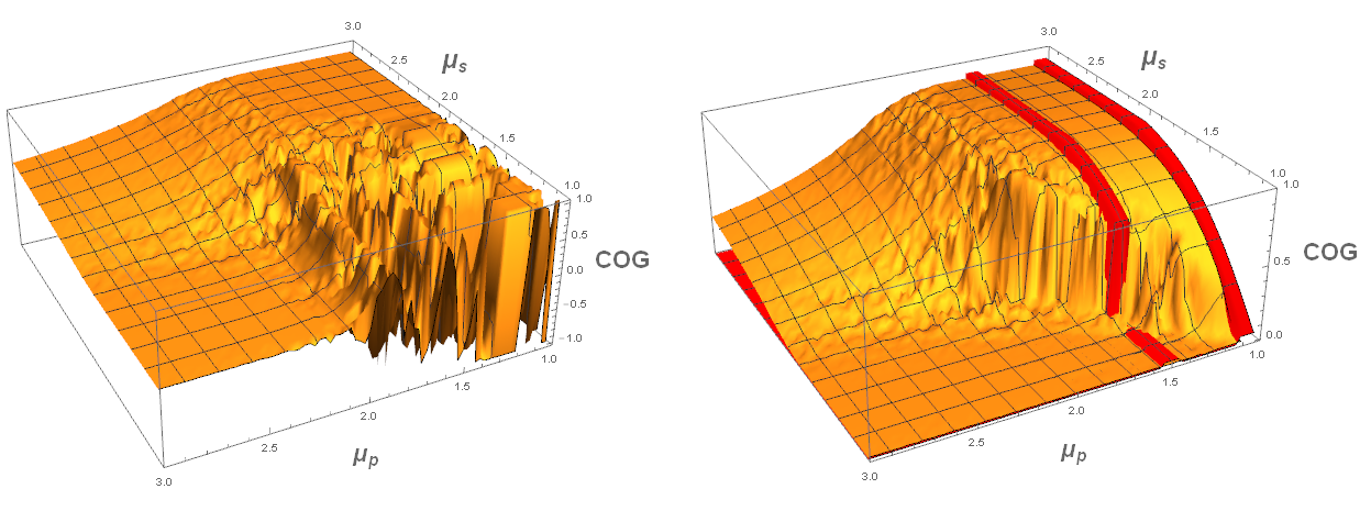
Figure 1: (Color online) COG as a function of the inverse power-law indexes $\mu_{S}$ and $\mu_{P}$. Left panel: The time sequence of length $L$ is divided into $L/T_{W}$ intervals of length $T_{W}$. The cross-correlation function of Eq. (6) is evaluated for each interval and the landscape is obtained plotting the mean of the resulting distribution of values. Right panel: The times $t_{i}$ of Eq. (6) are the times of event occurrence and the landscape is obtained by plotting the mean of the resulting distribution of values. The exact prediction of Eqs. (10) and (11) is shown by the two red lines.

We begin to address the limitation of a single time series by describing how the S-system is stimulated. Recalling Eq. (1), we note that there are two parameters that can be perturbed: $\mu$ and $T$. Since $\mu$ quantifies the complexity of the system, it is reasonable to expect that it can be forced to change only in response to very strong stimulation. A non-invasive perturbation, therefore, is expected to only change $T$. This restriction is in keeping with the dynamical approach to LRT used in silvestri09 , to design the GLRT aquino10 ; aquino11 that led to such remarkably good agreement with experimental observation.

The P-system exerts its influence on the S-system as follows: if S has an event at time $t$ and if its next laminar region is assigned a value with the same sign as $\xi_{P}(t)$, then S is perturbed so that its next laminar region tends to be longer, by assigning to its parameter $T$ in Eq. (1) the value $T_{+}=T(1+\epsilon)$. On the contrary, if the next laminar region of S has a value with the opposite sign to that of $\xi_{P}(t)$, then the value $T_{-}=T(1-\epsilon)$ is used, thus tending to make the next laminar region shorter.

In order to assess the influence of P on S for a single time series, using this perturbation procedure, it is natural to consider a time window of size $T_{W}$ and analyze the time averaged cross-correlation function:

$$C\left(t_{0},T_{W}\right)\equiv\frac{1}{T_{W}}\int_{t_{0}}^{t_{0}+T_{W}}dt^{\prime}\xi_{S}(t^{\prime})\xi_{P}(t^{\prime}).$$ (6)

By moving the starting point $t_{0}$ of the window and evaluating $C$, a density plot for the time averaged cross-correlation can be created as a function of the power-law indices. A measure of the influence of the P-system on the S-system is the center of gravity (COG) of this density plot. In the domain $1<\mu_{S},\mu_{P}<2$, the COG of the density plot is erratic; in sharp contrast with the smooth behavior found in the calculations of the cross-correlation function in this region obtained using ensemble distribution functions by Aquino et al. aquino10 ; aquino11 . This is clearly shown in the left panel of Fig. (1), where $C/\epsilon$ is plotted as a function of $\mu_{S}$ and $\mu_{P}$. It is worth noting that different realizations of the figure lead to different landscapes in the non-ergodic quadrant. The reasons behind this behavior will become clear shortly.

The main contribution of this Letter has two parts. The first part is a new data processing prescription that enables one to eliminate the erratic behavior observed in the left panel of Fig. (1) and produce the smooth behavior of the right panel. In the second part we provide a theoretical justification for this prescription and calculate the asymptotic cross-correlation function analytically.

The prescription is to locate the beginning $t_{0}$ of the window at which each $C$ is evaluated on an event of either the perturbing or the perturbed system.

We now turn our attention to presenting the theoretical foundations that led to the data processing prescription given above. We start by considering the following random quantity: $\overline{\xi_{S}}=\int_{0}^{t}dt^{\prime}\xi_{S}(t^{\prime})/t$ based on different realizations of the unperturbed $\xi_{S}$ that was prepared so as to have an event at $t_{0}=0$. Notice that the beginning of the window is always located at $t=0$, in contrast to Eq.(6). In the case of $\mu_{S}<2$, it was shown by performing ensemble averages annunziato01 that $\overline{\xi_{S}}$ is characterized by the Lamperti probability density function lamperti58 :

$$\Pi(\overline{\xi_{S}})=\frac{2}{\pi}\frac{\left(1-\overline{\xi_{S}}^{2}\right)^{\alpha-1}sin\pi\alpha}{\left(1-\overline{\xi_{S}}\right)^{2\alpha}+\left(1+\overline{\xi_{S}}\right)^{2\alpha}+\left(1-\overline{\xi_{S}}^{2}\right)^{\alpha}cos\pi\alpha},$$ (7)

where $\alpha$ is $\mu-1$. Whose graph is depicted as the symmetric curve in Fig. (2). We notice that this distribution is clearly non-ergodic as a single realization is most probably located around 1 or -1, while the ensemble average is zero.

We now consider the time-averaged quantity $\overline{\xi}\equiv\frac{1}{T_{W}}\int_{0}^{T_{W}}dt\xi_{S}(t)\xi_{P}(t),$ that is Eq. (6) when $t_{0}=0$ and we employ the same procedure followed in the calculation of $\overline{\xi_{S}}$. Bologna et al bologna10 , as well as Akimoto akimoto12 , demonstrated that the resulting distribution is a skewed Lamperti distribution given by:

$$\Pi(\overline{\xi})=\frac{2}{\pi}\frac{\left(1-\overline{\xi}^{2}\right)^{\alpha-1}sin\pi\alpha}{\left(1-\overline{\xi}\right)^{2\alpha}\eta+\left(1+\overline{\xi}\right)^{2\alpha}\frac{1}{\eta}+\left(1-\overline{\xi}^{2}\right)^{\alpha}cos\pi\alpha}.$$ (8)

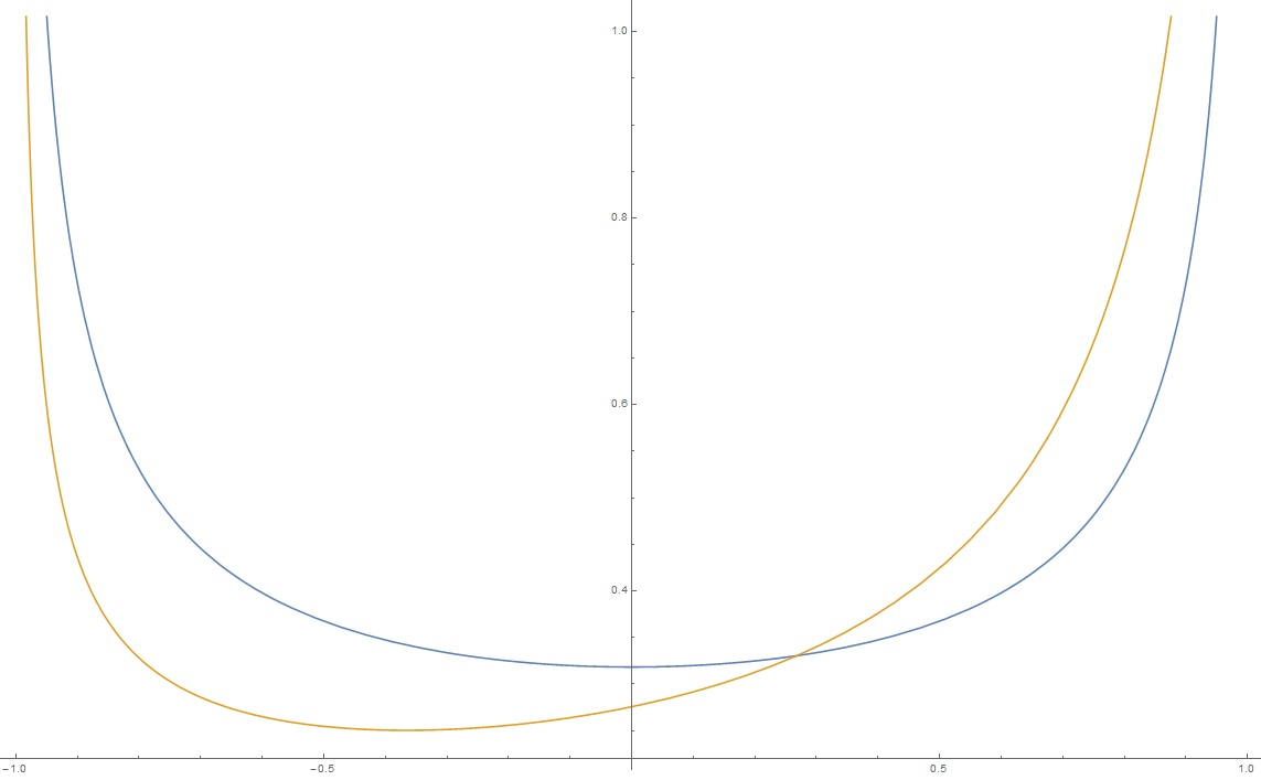
Figure 2: (Color online) Unperturbed ($\epsilon=0$) and perturbed ($\epsilon=0.5$) Lamperti distributions with $\mu=1.5$

The parameter $\eta$ is responsible for the asymmetry of the curve in Fig. (2) and is related to the intensity of the perturbation $\epsilon$ by:

$$\eta\equiv\left(\frac{1-\epsilon}{1+\epsilon}\right)^{\alpha}.$$ (9)

The COG of the density plot is given by

$$B\left(\mu_{P},\mu_{S}\right)=\epsilon\frac{1-\left(\frac{1-\epsilon}{1+\epsilon}\right)^{\mu_{S}-1}}{1+\left(\frac{1-\epsilon}{1+\epsilon}\right)^{\mu_{S}-1}}$$ (10)

These results are exact for $t_{0}=0$, but, as we discussed, in many real applications the distribution of $C$ is necessarily determined from a moving time window. In order to understand how these results can be useful in the latter case, we make some intuitive observations, followed by additional theory. We already noted that, when $\mu<2$, the mean length of the laminar regions of a system is infinity. This explains why we obtain the erratic plot in the left panel of Fig. (1): for most of the duration of the time series there are no events, thus the cross-correlation is either 1 or -1. This fact can be exploited to obtain the regular behavior of the right panel of Fig. (1): when one of the two systems has an event, it is most probably embedded in a long laminar region of the other system. If the P-system has an event, then it is most likely embedded in a long laminar region of the S-system. In this case the resulting value of $C$ follows the statistics of the unperturbed Lamperti distribution given by Eq. (7), as the S-system has no influence on the P-system and the latter is non-ergodic. If the S-system has an event, then it is most likely embedded in a long laminar region of the P-system, which is equivalent to saying that S is subject to constant stimulation. In this case the computed value of $C$ follows the statistics of the perturbed Lamperti distribution given by Eq. (8). The probability $W_{S}$ of having an event in S at time $t$ is given by:

$$W_{S}(t)=\frac{R_{S}(t)}{R_{S}(t)+R_{P}(t)},$$ (11)

with $R(t)$ given by Eq. (3) with the $\mu$ of the corresponding system. The probability $W_{P}$ can be obtained from (11) by exchanging the roles of S and P. When $t\rightarrow\infty$, if $\mu_{S}>\mu_{P}$, we have $W_{S}=1$ and $W_{P}=0$; if $\mu_{S}<\mu_{P}$ then $W_{S}=0$ and $W_{P}=1$. As a side note we observe that this argument implies that the perturbed system does not respond asymptotically to simple perturbations, which corresponds to the phenomenon of habituation.

The red stripes superimposed on the numerical calculations in the right panel of Fig (1) are determined using Eqs. (10) and (11) and show excellent agreement with the numerical simulations. The above derivation is valid also in the case in which one of the systems is ergodic and the other is not ergodic: in the long time limit, only the former has events. This fact and the considerations above imply that, in complete agreement with PCM, the response of an ergodic system to a non-ergodic system is maximal. On the other hand, the response of a non-ergodic system to an ergodic system vanishes. In the case in which both sytems are ergodic, the above theory is not applicable, but, given the equivalence (by definition) of ensemble averages and time averages, in this case we again recover the results of PCM, as expected.

In conclusion, this Letter extends GLRT, by indicating how to apply PCM to single time series and determining how information is transfered between systems. The issue was addressed at a formal level, in order to provide results that are valid for a range of systems, that is, systems in the physical, social and life sciences. These guidelines can be used to apply the PCM to real experimental data, so as to assess, for instance, the response of the brain to noninvasive stimuli, with the condition of analyzing the crucial renewal events of the brain that are detectable and observable, as shown by allegrini09 ; allegrini07 . In the literature there is an increasing interest in criticality as well as in intelligence-induced criticality chialvo10 ; haimovici13 ; beggs15 ; couzin07 ; plenz14 and the theory along with the practical rules to detect correlation in the non-ergodic case, afforded by this Letter, are expected to contribute to the advance of this field of research.

acknowledgment NP, DL and GP thank Welch for financial support through Grant No. B-1577 and ARO for financial support through Grant W911NF-15-1-0245.

References

- (1) G. Aquino, M. Bologna, P. Grigolini and B.J. West, Phys. Rev. Lett. 105, 040601-1 (2010).
- (2) G. Aquino, M. Bologna, B.J. West and P. Grigolini, Phys. Rev. E 83, 051130-1 (2011).
- (3) N. Wiener, Ann. NY Acad. Sci (YEAR).
- (4) R.M. Neumann, The Journal of Chemical Physics 66, 870 (1977).
- (5) G. Holloway, Entropy 11, 390 (2009).
- (6) R. L. Carhart-Harris, R. Leech, P.J. Hellyer, M. Shanahan, A. Feilding, E. Tagliazucchi, D.R. Chialvo and D. Nutt, Front. Hum. Neurosci., 03 February 2014 http://dx.doi.org/10.3389/fnhum.2014.00020
- (7) J.M. Beggs and D. Plenz, J. Neurosci. 23, 11167 (2003); O. Kinouchi et al., Nature Phys. 2, 348 (2006).
- (8) B.J. West and P. Grigolini, Complex Webs, Anticipating the Improbable, Cambridge University Press, cambridge, UK (2011).
- (9) I. M. Sokolov et al., Physica (Amsterdam) 302A, 268 (2001); I.M. Sokolov and J. Klafter, Phys. Rev. Lett. 97, 140602 (2006); I.M. Sokolov, Phys. Rev. E 73, 067102 (2006).
- (10) F. Barbi et al., Phys. Rev. Lett. 95, 220601 (2005).
- (11) A. Weron, et al., Phys. Rev. E 77, 036704 (2008).
- (12) M. Magdziarz et al., Phys. Rev. Lett. 101, 210601 (2008).
- (13) Y. Yu et al., Phys. Rev. Lett. 94, 108103 (2005).
- (14) D. L. Gilden, Psychological Review 108, 33-56 (2001).
- (15) G. C. Van Orden, J. G. Holden, M. T. Turvey, Journal of Experimental Psychology:General 134,117-123 (2005).
- (16) S. Farrell, E.-J. Wagenmakers, R. Ratcliff, Psychonomic Bulletin & Review 13, 737-741 (2006).
- (17) P. Allegrini, P. Paradisi, D. Menicucci, M. Laurino, A. Piarulli,A. Gemignani, Phys. Rev. E 92, 032808, 1-9 (2015).
- (18) J. K. Ochab, J. Tyburczyk, E. Beldzik, D. R. Chialvo, A. Domagalik, M. Fafrowicz, E. Gudowska-Nowak, T. Marek, M. A. Nowak, H. Oginska, J. Szwed, PLOS ONE 9, e107542, 1-12 (2014).
- (19) P. Allegrini, D. Menicucci, R. Bedini, L. Fronzoni, A. Gemignani, P. Grigolini, B. J. West, P. Paradisi, Phys. Rev. E 80, 061914, 1-13 (2009).
- (20) M. Annunziato, P. Grigolini, B. J. West, Phys. Rev. E 64, 011107, 1-13 (2001).
- (21) P. Allegrini, J. Bellazzini, G. Bramanti, M. Ignaccolo, P. Grigolini, and J. Yang, Phys. Rev. E 66, 015101-1 (2015).
- (22) W. Feller, An Introduction to Probability Theory and Its Applications, John Wiley & Sons, New York (1971).
- (23) M. Lukovic and P. Grigolini, J. Chem. Phys. 129, 184102, 1-11 (2008).
- (24) R. Kubo, M. Toda, and N. Hashitsume, Statistical Physics II: Nonequilibrium Statistical Mechanics, Springer-Verlag, Berlin (1985).
- (25) S. Burov et al., Phys. Chem. Chem. Phys 13, 1800-1812 (2011).
- (26) L. Silvestri, L. Fronzoni, P. Grigolini, P. Allegrini, Phys. Rev. Lett. 102, 014502, 1-4 (2009).
- (27) J. Lamperti, Trans. Am. Math. Soc. 88, 380 (1958).
- (28) M. Bologna,G. Ascolani, P. Grigolini, J. Math. Phys. 51, 043303, 1-17 (2010).
- (29) T. Akimoto, Phys. Rev. Lett. 108, 164101-1 (2012).
- (30) P. Allegrini, M. Bologna, P. Grigolini, B. J. West, Phys. Rev. Lett. 99, 010603, 1-4 (2007).
- (31) D. Chialvo, Nature Physics 6, 744-750 (2010).
- (32) A. Haimovici, E. Tagliazucchi, P. Balenzuela, D. R. Chialvo, Phys. Rev. Lett. 110, 178101, 1-4 (2013).
- (33) J. Beggs, Phys. Rev. Lett. 114, 220001, 1-1 (2015).
- (34) I. Couzin, Nature (London) 445, 715 (2007).
- (35) D. Plenz and E. Niebur (Editors), Criticality in Neural Systems, Wiley-VCH (2014).
- (36) G. Margolin and E. Barkai, J. Stat. Phys. 122, 137 (2006).
- (37) P. Allegrini, G. Aquino, P. Grigolini, L Palatella, A. Rosa, Phys. Rev. E 68, 1-11 056123 (2003).
- (38) E. Barkai, Phys. Rev. Lett. 90, 104101 (2003).