Abstract

We consider a three-Higgs doublet scenario in this paper, invariant under the discrete group $S_{3}$, and probe its high-scale validity by allowing the model parameters to evolve under renormalisation group. We choose two particular alignments of vacuum expectation values (vev) for our study, out of a set of several such possible ones. All three doublets receive non-zero vacuum expectation values in the first case, and in the second case, two of the doublets remain without vev. The constraints on the parameter space at low energy, including the measured value of the Higgs mass and the signal strengths, oblique corrections and also measurements of relic density and direct detection rates are juxtaposed with the conditions of vacuum stability, perturbativity and unitarity at various scales. We find that the scenario with three non-zero vevs is not valid beyond $10^{7}$ GeV, assuming no additional physics participates at the intermediate scales. On the contrary, the scenario with only one non-zero vev turns out to be a successful model for cold dark matter phenomenology, which also turns out to be valid up to the Planck scale at the same time. Stringent restrictions are obtained on the model parameter space in each case. Thus, the $S_{3}$ symmetric scalar sector emerges as an ultraviolet (UV) complete theory.

1 Introduction

The discovery of a scalar boson around 125 GeV[1, 2] has been the most important finding at the LHC so far. It has gradually unfurled that the newly discovered boson has properties largely consistent with the Standard Model (SM) Higgs[3, 4, 5]. There is however one pressing issue that a SM Higgs around 125 GeV leads to an instability in the electroweak vaccum around $10^{8-9}$ GeV if the top quark mass $(M_{t})$ and the strong coupling constant $(\alpha_{s})$ are on the upper edges of their respective uncertainty bands. A recent next-to-next-to-leading order (NNLO) study [6, 7] reports that absolute stability up to the Planck scale requires

$$M_{h}[\rm GeV]>129.4+1.4(\frac{M_{t}[\rm GeV]-173.1}{0.7})-0.5(\frac{\alpha_{s}(M_{Z})-0.1184}{0.0007})\pm 1.0_{th}$$ (1.1)

As a possible remedy to alleviate the vacuum stability problem, the SM Higgs can be made to couple to additional bosonic degrees of freedom. In such a case, the extra scalar loops contributing to the running of the Higgs coupling can generate the required positive contribution to prevent the Higgs self coupling from turning negative. Thus ensuring a stable Elecroweak vacuum (EW) up to the GUT and Planck scales, forms our main motivation to add new scalars to the theory. Apart from this, various cosmological and astrophysical evidences of Dark Matter (DM) also necessiate physics beyond the SM. Attempts have been made to explore the yet unknown particle nature of DM and the most successful proposal is that DM is constituted of Weakly Interacting Massive Particles (WIMPs)[8].

It is however not possible to predict the actual number of scalar doublets present in nature from fundamental principles. The discovered scalar resonance around 125 GeV could very well arise from a multiple scalar doublet scenario with the additional parameters arranged suitably to give to it, SM-like couplings to fermions and gauge bosons. Of course, detection of the extra scalars at the colliders is the only direct way to pin down on the exact scalar structure present. Nonetheless these extra scalars could be fingerprinted through their role in stabilizing and unitarizing of the scalar potential. Moreover, the scalars originating from the extra doublets could possible be successful canditates for DM. While studies combining together vacuum stability and DM phenomenology have been done in the past in context of two-Higgs doublet models (2HDM)[9], these could be generalized to a higher number of doublets as well. There has been a rising interest in three-Higgs doublet models (3HDM) in the recent past[10, 12, 13, 14, 15, 16, 17, 18, 19, 20, 11]. The chief phenomenological motivation of which is that the existence of three scalar doublets, replicating the three fermion families, sheds light on the flavor problem. 3HDMs have rather wide scalar spectrum. In fact, invariance under SU(2) $\times$ U(1) tells us that there are four neutral scalars, and a pair of charged scalars obtainable from a generic 3HDM. It is reminded that 3HDMs come in various types, depending upon the global symmetry present. One of them is the 3HDM endowed with a global $S_{3}$ symmetry[21, 22, 23, 24, 25, 26]. This $S_{3}$ symmetry is already important from the perspective of flavor, it reproduces the lepton masses and mixings accurately [27, 28, 29, 30, 31, 32]. The scalar sector is also interesting since there is an economy of parameters compared to a more generic 3HDM. In fact the eight dimensionless parameters can be fully traded off in favour of the seven masses and one mixing angle. The $S_{3}$-symmetric scalar sector has spurred some investigation in the past, and some standalone studies related to DM phenomenology have also occurred[33]. However, the present study is mainly directed towards analysing the Higgs sector, and, it includes the following features which have not been highlighted before.

• We derive the renormalisation group equations at one-loop for the dimensionless parameters in an $S_{3}$ symmetric Higgs potential. Using these, we probe high-scale behaviour of the scalar potential. That is, we evolve the scalar quartic couplings and require that the model remains perturbative and keeps vacuum stability intact at each intermediate energy scale. Through this exercise, we try to identify the parameter space at the input scale that keeps the model valid till very high scales.

• Electroweak Symmetry Breaking (EWSB) is triggered when one or more doublet receives a vacuum expectation value (vev). While several such configurations of the vevs can be there in principle, we consider two such cases which not only are more relevant from the phenomenological point of view, but also demonstrative of the high-scale validity of the $S_{3}$ potential. For instance, we analyse a ’two inert doublet’ scenario where only one doublet gets a vev, and predicts existence of stable scalars through some remnant symmetry. This scenario thus stands as a potential canditate for describing DM.

• The parameter space allowing for high-scale validity is also subject to various low energy constraints, i.e., the ones originating from the oblique S, T and U parameters, signal strength measurements for the 125 GeV Higgs, and also DM searches.

This paper is organized as follows. In Section 2, we briefly discuss the salient features of the model, particularly the scalar and Yukawa sectors. The various constraints taken are listed in Section 3. The numerical results so obtained are detailed in Section 4, and finally, we summarize in Section 5. Relevant expressions and equations can be found in the Appendix Appendix..

2 The $S_{3}$ symmetric three-Higgs-doublet model ($S_{3}$HDM) in brief.

2.1 Scalar sector.

The scalar sector consists of three scalar doublets $\phi_{1}$, $\phi_{2}$ and $\phi_{3}$. The most general renormalizable scalar potential consistent with the gauge and $S_{3}$ symmetries can be cast as [34],

$$V(\phi) = \mu_{11}^{2}(\phi_{1}^{\dagger}\phi_{1}+\phi_{2}^{\dagger}\phi_{2})+\mu_{33}^{2}\phi_{3}^{\dagger}\phi_{3}$$ (2.1a)

$$+\lambda_{1}(\phi_{1}^{\dagger}\phi_{1}+\phi_{2}^{\dagger}\phi_{2})^{2}+\lambda_{2}(\phi_{1}^{\dagger}\phi_{2}-\phi_{2}^{\dagger}\phi_{1})^{2}+\lambda_{3}\left\{(\phi_{1}^{\dagger}\phi_{2}+\phi_{2}^{\dagger}\phi_{1})^{2}+(\phi_{1}^{\dagger}\phi_{1}-\phi_{2}^{\dagger}\phi_{2})^{2}\right\}$$

$$+\lambda_{4}\left\{(\phi_{3}^{\dagger}\phi_{1})(\phi_{1}^{\dagger}\phi_{2}+\phi_{2}^{\dagger}\phi_{1})+(\phi_{3}^{\dagger}\phi_{2})(\phi_{1}^{\dagger}\phi_{1}-\phi_{2}^{\dagger}\phi_{2})+{\rm h.c.}\right\}$$

$$+\lambda_{5}(\phi_{3}^{\dagger}\phi_{3})(\phi_{1}^{\dagger}\phi_{1}+\phi_{2}^{\dagger}\phi_{2})+\lambda_{6}\left\{(\phi_{3}^{\dagger}\phi_{1})(\phi_{1}^{\dagger}\phi_{3})+(\phi_{3}^{\dagger}\phi_{2})(\phi_{2}^{\dagger}\phi_{3})\right\}$$

$$+\lambda_{7}\left\{(\phi_{3}^{\dagger}\phi_{1})(\phi_{3}^{\dagger}\phi_{1})+(\phi_{3}^{\dagger}\phi_{2})(\phi_{3}^{\dagger}\phi_{2})+{\rm h.c.}\right\}+\lambda_{8}(\phi_{3}^{\dagger}\phi_{3})^{2}\,.$$

A 3HDM is usually known to have CP violating phases [35] in the scalar sector. For example a complex $\lambda_{4}$ and $\lambda_{7}$ in this case leads to CP non-conservation, although the phases are severely constrained by measurements of Electric Dipole Moment of the Neutron (EDMN)[36]. The high-scale stability of a 2HDM is found intact regardless of the CP phase[37]. Thus, the overall conclusions regarding validity of the $S_{3}$HDM at high scales is expected to remain unaffected by the introduction of CP phases. So we choose $\lambda_{4}$ and $\lambda_{7}$ to be real henceforth.

Electro-Weak Symmetry Breaking (EWSB) assigns vacuum expectation values (vevs) $v_{1}$, $v_{2}$ and $v_{3}$ to the doublets $\phi_{1}$, $\phi_{2}$ and $\phi_{3}$ respectively. However, they all are not independent as the $S_{3}$ invariance forces relationships among them through the minimization conditions below,

$$2\mu_{11}^{2} = -2\lambda_{1}(v_{1}^{2}+v_{2}^{2})-2\lambda_{3}(v_{1}^{2}+v_{2}^{2})-v_{3}\{6\lambda_{4}v_{2}+(\lambda_{5}+\lambda_{6}+2\lambda_{7})v_{3}\}\,,$$ (2.2a)

$$2\mu_{11}^{2} = -2\lambda_{1}(v_{1}^{2}+v_{2}^{2})-2\lambda_{3}(v_{1}^{2}+v_{2}^{2})-\frac{3v_{3}}{v_{2}}\lambda_{4}(v_{1}^{2}-v_{2}^{2})-(\lambda_{5}+\lambda_{6}+2\lambda_{7})v_{3}^{2}\,,$$ (2.2b)

$$2\mu_{33}^{2} = \lambda_{4}\frac{v_{2}}{v_{3}}(v_{2}^{2}-v_{1}^{2})-(\lambda_{5}+\lambda_{6}+2\lambda_{7})(v_{1}^{2}+v_{2}^{2})-2\lambda_{8}v_{3}^{2}\,.$$ (2.2c)

The self-consistency of Eqs. (2.2a) and (2.2b) gives rise to the following possibilities,

$$\lambda_{4} = 0\,,$$ (2.3a)

$${\rm or,}~{}~{}v_{1} = \sqrt{3}v_{2}\,,$$ (2.3b)

$${\rm or,}~{}~{}v_{1} = v_{2}=0,~{}v_{3}=246~{}\rm GeV\,.$$ (2.3c)

The first case causes a physical scalar to turn massless as reported in [38]. This directs us towards the other two cases that we outline below.

The doublets are parameterized in the following fashion,

$$\phi_{i}=\frac{1}{\sqrt{2}}\begin{pmatrix}\sqrt{2}w_{i}^{+}\\ v_{i}+h_{i}+iz_{i}\end{pmatrix}~{}\rm{for}~{}\textit{i}=1,2,3.$$ (2.4)

The physical scalar spectrum of a generic CP-conserving 3HDM consists of three CP even neutral scalars, $H_{1}$, $H_{2}$ and $h$; two CP-odd neutral scalars $A_{1}$ and $A_{2}$; and two charged scalars $H_{1}^{+}$ and $H_{2}^{+}$. We define tan$\beta$ = $\frac{2v_{2}}{v_{1}}$ for Scenario A (Eqn.2.3b). For this vev-alignment, only two mixing angles $\alpha$ and $\beta$ are sufficient to parameterize the transformation matrices connecting the SU(2) eigenbasis to the physical basis, somewhat resembling a 2HDM. The model is more conveniently described in terms of physical quantities like masses and mixing angles. The eight $\lambda_{i}$ can be traded for the seven masses and the mixing angle $\alpha$ (See [39] for definition.) using the following equations,

$$\lambda_{1} = \frac{1}{2v^{2}\sin^{2}\beta}\left\{\left(m_{h}^{2}\cos^{2}\alpha+m_{H_{1}}^{2}\sin^{2}\alpha\right)+\left(m_{H^{+}_{1}}^{2}-m_{H^{+}_{2}}^{2}\cos^{2}\beta-\frac{1}{9}m_{H_{2}}^{2}\right)\right\}\,,$$ (2.5a)

$$\lambda_{2} = \frac{1}{2v^{2}\sin^{2}\beta}\left\{(m_{H^{+}_{1}}^{2}-m_{A_{1}}^{2})-(m_{H^{+}_{2}}^{2}-m_{A_{2}}^{2})\cos^{2}\beta\right\}\,,$$ (2.5b)

$$\lambda_{3} = \frac{1}{2v^{2}\sin^{2}\beta}\left(\frac{4}{9}m_{H_{2}}^{2}+m_{H^{+}_{2}}^{2}\cos^{2}\beta-m_{H^{+}_{1}}^{2}\right)\,,$$ (2.5c)

$$\lambda_{4} = -\frac{2}{9}\frac{m_{H_{2}}^{2}}{v^{2}}\frac{1}{\sin\beta\cos\beta}\,,$$ (2.5d)

$$\lambda_{5} = \frac{1}{v^{2}}\left\{\frac{\sin\alpha\cos\alpha}{\sin\beta\cos\beta}\left(m_{H_{1}}^{2}-m_{h}^{2}\right)+2m_{H^{+}_{2}}^{2}+\frac{1}{9}\frac{m_{H_{2}}^{2}}{\cos^{2}\beta}\right\}\,,$$ (2.5e)

$$\lambda_{6} = \frac{1}{v^{2}}\left(\frac{1}{9}\frac{m_{H_{2}}^{2}}{\cos^{2}\beta}+m_{A_{2}}^{2}-2m_{H^{+}_{2}}^{2}\right)\,,$$ (2.5f)

$$\lambda_{7} = \frac{1}{2v^{2}}\left(\frac{1}{9}\frac{m_{H_{2}}^{2}}{\cos^{2}\beta}-m_{A_{2}}^{2}\right)\,,$$ (2.5g)

$$\lambda_{8} = \frac{1}{2v^{2}\cos^{2}\beta}\left\{\left(m_{h}^{2}\sin^{2}\alpha+m_{H_{1}}^{2}\cos^{2}\alpha\right)-\frac{1}{9}m_{H_{2}}^{2}\tan^{2}\beta\right\}\,.$$ (2.5h)

We also put forth the Scenario B (Eqn.2.3c) as an alternate symmetry breaking pattern. In this case, $\phi_{3}$ is the only active doublet, which is in fact a singlet under $S_{3}$. Consequently, all the fermions couple to $\phi_{3}$ alone and thus they too are $S_{3}$-singlets. The remaining doublets $\phi_{1}$ and $\phi_{2}$ remain inert. A $Z_{2}$ symmetry is found unbroken for $\lambda_{4}$ = 0, and it forbids mixing among scalars coming from different doublets thus enabling one to express the doublets directly in terms of the physical fields as,

$$\phi_{3}=\frac{1}{\sqrt{2}}\begin{pmatrix}\sqrt{2}w^{+}\\ v+h+iz\end{pmatrix}~{}$$ (2.6)

$$\phi_{i}=\frac{1}{\sqrt{2}}\begin{pmatrix}\sqrt{2}H_{i}^{+}\\ H_{i}+iA_{i}\end{pmatrix}~{}\rm{for}~{}\textit{i}=1,2.$$ (2.7)

With $m^{2}_{h}$ = $2\lambda_{8}v^{2}$ now, the $S_{3}$ symmetry leads to a mass degeneracy in the inert sector,

$$m^{2}_{H_{1}} = m^{2}_{H_{2}}=\mu^{2}_{11}+\frac{1}{2}\lambda_{L}v^{2}$$ (2.8)

$$m^{2}_{A_{1}} = m^{2}_{A_{2}}=\mu^{2}_{11}+\frac{1}{2}\lambda_{A}v^{2}$$ (2.9)

$$m^{2}_{H^{+}_{1}} = m^{2}_{H^{+}_{2}}=\mu^{2}_{11}+\frac{1}{2}\lambda_{5}v^{2}$$ (2.10)

Here $-\lambda_{L}v$ and $-\lambda_{A}v$ denote the $H_{1}$-$H_{1}$-$h$ and $A_{1}$-$A_{1}$-$h$ couplings respectively. This mass degeneracy can be lifted in this case, for example, by introducing an $S_{3}$ breaking quadratic term of the form $-\mu_{12}^{2}(\phi_{1}^{\dagger}\phi_{2}+\phi_{2}^{\dagger}\phi_{1})$. However, implications of a broken $S_{3}$ symmetry are outside the scope of this paper.

It is interesting to probe the parameter space arising out of such a vev alignment by proposing $H_{1}$ and $H_{2}$ as possible DM canditates. For the $S_{3}$HDM to qualify as a good DM model, its predictions of relic-density and direct detection rates must be matched against corresponding experimental data. We arrange for the hierarchy $m_{H_{1}}$ $\textless$ $m_{A_{1}}$, $m_{H^{+}_{1}}$ throughout our numerical analysis ($H_{1}$ and $A_{1}$ are similar to each other in terms of the masses and couplings, the only difference being the sign of $\lambda_{7}$. Thus a flip in the sign of $\lambda_{7}$ would tantamount to interchanging $H_{1}$ and $A_{1}$. In that case, $A_{1}$ would be the DM candiate and the hierarchy required would be $m_{A_{1}}$ $\leq$ $m_{H_{1}},m_{H^{+}_{1}}$. The overall physics thus remains unchanged.). LEP constraints on the direct search for charged and pseudoscalar Higgs bosons are evaded by taking $m_{H^{+}_{i}}$ and $m_{A_{i}}$ $\textgreater$ 100 GeV[40]. Similar to the previous case, we describe the model parameter space in terms of the physical parameters $\{$ $\lambda_{1}$, $\lambda_{2}$, $\lambda_{3}$, $m_{H_{1}},m_{A_{1}},m_{H^{+}_{1}}$, $\lambda_{L}$ $\}$.

Our main motivation is to study the high-scale stability of the $S_{3}$HDM for the two different vev assignments discussed above. In doing that we juxtapose the constraints coming from oblique parameters, Higgs signal strengths in the first case, and also the ones coming from relic-density and direct detection in the second case. In principle there can be other such vev configurations as well, and our choice is not exhaustive in that sense. Nonetheless, this paper takes into account two representative cases. The first one defines an active 3HDM scenario, i.e, when all three $\phi_{1}$, $\phi_{2}$ and $\phi_{3}$ receive non-zero vevs. The second one describes an inert scenario, where these inert scalars do not mix with the 125 GeV Higgs that comes from $\phi_{3}$.

2.2 Yukawa Sector.

The most general Yukawa lagrangian consistent with the gauge and $S_{3}$ symmetries, for the up-type quarks is given by,

$$-\mathscr{L}_{Y}^{u} = \hbox{}y_{1}^{u}\Big{(}\bar{Q}_{1}\tilde{\phi}_{3}u_{1R}+\bar{Q}_{2}\tilde{\phi}_{3}u_{2R}\Big{)}+y_{2}^{u}\Big{\{}\Big{(}\bar{Q}_{1}\tilde{\phi}_{2}+\bar{Q}_{2}\tilde{\phi}_{1}\Big{)}u_{1R}+\Big{(}\bar{Q}_{1}\tilde{\phi}_{1}+\bar{Q}_{2}\tilde{\phi}_{2}\Big{)}u_{2R}\Big{\}}$$ (2.11)

$$\hbox{}+y_{3}^{u}\bar{Q}_{3}\tilde{\phi}_{3}u_{3R}+y_{4}^{u}\bar{Q}_{3}\Big{(}\tilde{\phi}_{1}u_{1R}+\tilde{\phi}_{2}u_{2R}\Big{)}+y_{5}^{u}\Big{(}\bar{Q}_{1}\tilde{\phi}_{1}+\bar{Q}_{2}\tilde{\phi}_{2}\Big{)}u_{3R}+{\rm h.c.}$$

The lower component of the $SU(2)$ doublets of Higgs multiplets are uncharged in the convention we use. A standard abbreviation reads $\tilde{\phi}_{i}=i\sigma_{2}\phi_{i}^{*}$. The Yukawa couplings of the $d_{R}$ quarks can be obtained by replacing $u_{iR}$ by $d_{iR}$, $y_{i}^{u}$ by $y_{i}^{d}$, and $\tilde{\phi}_{i}$ by $\phi_{i}$ in $\mathscr{L}_{Y}^{u}$ and similarly for leptons. The Yukawa couplings are in general complex, which can be responsible for $CP$ violation. More elaborate discussions on $S_{3}$ symmetric Yukawa textures can be found in [42, 43, 44, 45].

After symmetry breaking, the mass matrix that arises in the up-type quark sector is the following, (In the $u,c,t$ basis):

$${\cal M}_{u}=\begin{pmatrix}(y_{1}^{u}v_{3}+y_{2}^{u}v_{2})/\sqrt{2}&y_{2}^{u}v_{1}/\sqrt{2}&y_{5}^{u}v_{1}/\sqrt{2}\\ y_{2}^{u}v_{1}/\sqrt{2}&y_{1}^{u}v_{3}-y_{2}^{u}v_{2}/\sqrt{2}&y_{5}^{u}v_{2}/\sqrt{2}\\ y_{4}^{u}v_{1}/\sqrt{2}&y_{4}^{u}v_{2}/\sqrt{2}&y_{3}^{u}v_{3}/\sqrt{2}\\ \end{pmatrix}\,,\qquad{\rm with~{}}v_{1}=\surd 3v_{2}\,.$$ (2.12)

The texture is of the same form for the down-type quarks and charged leptons. In principle, one can retain all the paramaters in the Yukawa matrix and fine-tune them appropriately in order to reproduce the correct fermion masses and mixings. However that would make the analysis using RG complicated and unwieldy and hence, we look for a simplification. Choosing $y_{4}^{u}$, $y_{5}^{u}$ = 0 brings ${\cal M}_{u}$ to a 2 $\times$ 2 $\oplus$ 1 $\times$ 1 block-diagonal form. The quark masses in the SM can be straightforwardedly reproduced by diagonalising the remaining the 2 $\times$ 2 block and then tuning the parameters appropriately. For example, the choice $y_{1}^{u}$ $\textless$ $y_{2}^{u}$ $\textless$ $\textless$ $y_{3}^{u}$ reproduces the observed up-type quark mass hierarchy. The advantage of this choice is that only $y_{3}^{u}$ = $\frac{v}{v_{3}}y^{SM}_{t}$ gets a value large enough to cast an impact on the RG evolution, where $y^{SM}_{t}$ is the SM t-quark Yukawa coupling and, all other Yukawa couplings have a negligible bearing. In addition, even if we invoke a non-zero $y_{4}^{u}$ and $y_{5}^{u}$, the observed quark-mixings will always render them small. Exactly this approximation is applied to the bottom quark and lepton sectors also. It is easy to see that then $y_{3}^{u}$: $y_{3}^{b}$: $y_{3}^{l}$ = $m_{t}$: $m_{b}$: $m_{\tau}$, i.e, this particular approximation scheme preserves the hierarchy of Yukawa couplings observed in the SM. Hence we infer that only the $t$-quark can contribute significantly to the beta functions through the parameter $y_{3}^{u}$ and the effect of all other fermions can be safely neglected in this context. Thus effectively with only one Yukawa into the picture, as far as high-scale stability is concerned, it becomes easier to throw light on the scalar sector.

In the inert case, all the fermion generations are $S_{3}$-singlets and hence couple only to $\phi_{3}$.

3 Constraints imposed.

Parameter space of the scenario at hand is surveyed throughly by generating random model-points in the $\{$tan$\beta,m_{H^{+}_{1}},m_{H^{+}_{2}},m_{A_{1}},m_{A_{2}},m_{H_{1}},m_{H_{2}},c_{\beta-\alpha}$ $\}$ basis in scenario A and, $\{\lambda_{1},\lambda_{2},\lambda_{3},m_{H_{1}},m_{A_{1}},m_{H^{+}_{1}},\lambda_{L}\}$ in scenario B. We discuss below the various theoretical and experimental constraints imposed to shape the results.

3.1 Theoretical constraints.

The $S_{3}$HDM remains a calculable theory if the model parameters fulfil the respective perturbativity constraints, $|\lambda_{i}|\leq 4\pi$, $|y_{t}|,|g_{1}|,|g_{2}|,|g_{3}|\leq\sqrt{4\pi}$. A more stringent choice is to demand all of the couplings $\leq\sqrt{4\pi}$. We however stick to 4$\pi$, since this projects out the maximally allowed parameter space.

The 2$\rightarrow$2 amplitude matrix corresponding to scattering of the longitudinal components of the gauge bosons can be mapped to a corresponding matrix for the scattering of the goldstone bosons[46, 47, 48, 49]. The theory respects unitarity if each eigenvalue of the aforementioned amplitude matrix does not exceed 8$\pi$.

$$|a_{i}^{\pm}|,~{}|b_{i}|\leq 8\pi,~{}\mbox{for}~{}i=1,2,\ldots,6\,.$$ (3.1)

The expressions for the individual eigenvalues[39] in terms of quartic couplings are given below :

$$a^{\pm} = \left(\lambda_{1}-\lambda_{2}+\frac{\lambda_{5}+\lambda_{6}}{2}\right)\pm\sqrt{\left(\lambda_{1}-\lambda_{2}+\frac{\lambda_{5}+\lambda_{6}}{2}\right)^{2}-4\left\{(\lambda_{1}-\lambda_{2})\left(\frac{\lambda_{5}+\lambda_{6}}{2}\right)-\lambda_{4}^{2}\right\}}\,,$$ (3.2a)

$$b^{\pm} = \left(\lambda_{1}+\lambda_{2}+2\lambda_{3}+\lambda_{8}\right)\pm\sqrt{\left(\lambda_{1}+\lambda_{2}+2\lambda_{3}+\lambda_{8}\right)^{2}-4\left\{\lambda_{8}(\lambda_{1}+\lambda_{2}+2\lambda_{3})-2\lambda_{7}^{2}\right\}}\,,$$ (3.2b)

$$c^{\pm} = \left(\lambda_{1}-\lambda_{2}+2\lambda_{3}+\lambda_{8}\right)\pm\sqrt{\left(\lambda_{1}-\lambda_{2}+2\lambda_{3}+\lambda_{8}\right)^{2}-4\left\{\lambda_{8}(\lambda_{1}-\lambda_{2}+2\lambda_{3})-\frac{\lambda_{6}^{2}}{2}\right\}}\,,$$ (3.2c)

$$d^{\pm} = \left(\lambda_{1}+\lambda_{2}+\frac{\lambda_{5}}{2}+\lambda_{7}\right)\pm\sqrt{\left(\lambda_{1}+\lambda_{2}+\frac{\lambda_{5}}{2}+\lambda_{7}\right)^{2}-4\left\{(\lambda_{1}+\lambda_{2})\left(\frac{\lambda_{5}}{2}+\lambda_{7}\right)-\lambda_{4}^{2}\right\}}\,,$$ (3.2d)

$$e^{\pm} = \left(5\lambda_{1}-\lambda_{2}+2\lambda_{3}+3\lambda_{8}\right)$$ (3.2e)

$$\pm\sqrt{\left(5\lambda_{1}-\lambda_{2}+2\lambda_{3}+3\lambda_{8}\right)^{2}-4\left\{3\lambda_{8}(5\lambda_{1}-\lambda_{2}+2\lambda_{3})-\frac{1}{2}(2\lambda_{5}+\lambda_{6})^{2}\right\}}\,,$$

$$f^{\pm} = \left(\lambda_{1}+\lambda_{2}+4\lambda_{3}+\frac{\lambda_{5}}{2}+\lambda_{6}+3\lambda_{7}\right)$$ (3.2f)

$$\pm\sqrt{\left(\lambda_{1}+\lambda_{2}+4\lambda_{3}+\frac{\lambda_{5}}{2}+\lambda_{6}+3\lambda_{7}\right)^{2}-4\left\{(\lambda_{1}+\lambda_{2}+4\lambda_{3})\left(\frac{\lambda_{5}}{2}+\lambda_{6}+3\lambda_{7}\right)-9\lambda_{4}^{2}\right\}}\,,$$

$$h_{1} = \lambda_{5}+2\lambda_{6}-6\lambda_{7}\,,$$ (3.2g)

$$h_{2} = \lambda_{5}-2\lambda_{7}\,,$$ (3.2h)

$$h_{3} = 2(\lambda_{1}-5\lambda_{2}-2\lambda_{3})\,,$$ (3.2i)

$$h_{4} = 2(\lambda_{1}-\lambda_{2}-2\lambda_{3})\,,$$ (3.2j)

$$h_{5} = 2(\lambda_{1}+\lambda_{2}-2\lambda_{3})\,,$$ (3.2k)

$$h_{6} = \lambda_{5}-\lambda_{6}\,.$$ (3.2l)

In addition to the above, the scalar potential must be bounded from below in order to render the electroweak vacuum stable. Demanding absolute stability of the vacuum leads to the following conditions[39],

$$\rm vsc1:\lambda_{1} > 0\,,$$ (3.3)

$$\rm vsc2:\lambda_{8} > 0\,,$$ (3.4)

$$\rm vsc3:\lambda_{1}+\lambda_{3} > 0\,,$$ (3.5)

$$\rm vsc4:2\lambda_{1}+(\lambda_{3}-\lambda_{2}) > |\lambda_{2}+\lambda_{3}|\,,$$ (3.6)

$$\rm vsc5:\lambda_{5}+2\sqrt{\lambda_{8}(\lambda_{1}+\lambda_{3})} > 0\,,$$ (3.7)

$$\rm vsc6:\lambda_{5}+\lambda_{6}+2\sqrt{\lambda_{8}(\lambda_{1}+\lambda_{3})} > 2|\lambda_{7}|\,,$$ (3.8)

$$\rm vsc7:\lambda_{1}+\lambda_{3}+\lambda_{5}+\lambda_{6}+2\lambda_{7}+\lambda_{8} > 2|\lambda_{4}|\,.$$ (3.9)

This conditions can be arrived at by demanding the scalar potential remains positive along various directions in the field space in the $\phi_{i}\rightarrow\infty$ limit. We do not consider metastable vacua configurations in this paper [50, 51], which are expected to project a more relaxed parameter space in this context.

3.2 Oblique parameters.

The $S_{3}$HDM induces modification in the $S$, $T$ and $U$ parameters through the additional scalars participating in the loops of the gauge-boson self energies. One discerns the 3HDM contribution from the SM as,

$$S=S_{SM}+\Delta S$$ (3.10a)

$$T=T_{SM}+\Delta T,$$ (3.10b)

$$U=U_{SM}+\Delta U$$ (3.10c)

Here $\Delta S$, $\Delta T$ and $\Delta U$ denote the $S_{3}$HDM contributions. These have been derived following the approach outlined in[52]. Relevant expressions to can be found in the Appendix A. The central value is the contribution coming from the standard model with the reference values $m_{h,\rm{ref}}=125.0$ GeV and $M_{t,\rm{ref}}=173.1$ GeV where $M_{t}$ denotes the pole mass of the top quark. We have used 1$\sigma$ limits of $S$,$T$ and $U$ following [53].

3.3 Higgs Signal-strengths

The ATLAS and CMS collaborations have measured the production cross section for a $\sim$125 GeV Higgs multiplied by its branching ratios to various possible channels. The results so far are increasingly in favor of the SM predictions. An extended Higgs sector, such as the $S_{3}$HDM although can very well contain a scalar with mass around 125 GeV, but yet can potentially modify the signal strength predictions through its modified higgs-gauge boson and higgs-fermion couplings. For example, the $hVV$ and $hb\bar{b}$ couplings get scaled by sin($\beta-\alpha$) and $\frac{sin\alpha}{cos\beta}$ w.r.t the SM, in the case with three non-zero vevs. The loop induced decay widths to $\gamma\gamma$ and $Z\gamma$ final states are also modified. However, one can always arrange for $\alpha=\beta-\frac{\pi}{2}$ which reproduces exact SM couplings. This so called alignment limit is present in two-higgs doublet models as well[54]. We explore a case where this limit is not strictly enforced, rather sin$(\beta-\alpha)$ = 0.98 is taken. The reader is reminded that the tree level couplings of $h$ to fermions and gauge bosons remain identical to the SM in the presence of additional inert doublets.

In order to check the consistency of a 2HDM with the measured rates in various channels, we theoretically compute the signal strength $\mu^{i}$ for the $i$-th channel using the relation:

$$\mu^{i}=\frac{R_{\rm{prod}}\times R_{\rm{decay}}^{i}}{R_{\rm{width}}}~{}.$$ (3.11)

Here $R_{\rm{prod}}$, $R_{\rm{decay}}^{i}$ and $R_{\rm{width}}$ denote respectively the ratios of the theoretically calculated production cross section, the decay rate to the $i$-th channel and the total decay width for a $\sim$125 GeV Higgs to their corresponding SM counterparts. For our numerical analysis, we have taken gluon fusion to be the dominant production mode for the SM-like Higgs. The predicted signal-strengths to $ZZ$, $WW$, $b\bar{b}$ channels are in excellent agreement with the SM once the alignment limit is invoked. $\mu_{\gamma\gamma}$ still needs to be controlled since the charged scalars do not decouple from the theory in spite of an exact alignment (see Appendix C). In an exact-alignment scenario, the total width of $h$ hardly deviates from its SM value and $\mu_{\gamma\gamma}$ settles approximately to $\frac{\Gamma^{S_{3}\rm HDM}_{h\rightarrow\gamma\gamma}}{\Gamma^{\rm SM}_{h\rightarrow\gamma\gamma}}$. Latest measurements from ATLAS and CMS give $\mu_{\gamma\gamma}$ = $1.17^{+0.27}_{-0.27}$ and $1.12^{+0.24}_{-0.24}$ respectively [55, 56]. We use the cited limits at 2$\sigma$.

We make the passing remark that in-house codes have been employed to carry out the computations related to oblique parameters and signal strengths. In particular, the RG equations have been numerically solved by implementing the Runge-Kutta (RK4) algorithm in the same.

3.4 Dark matter relic density and direct detection

In the one active + two inert doublet case, we impose that the relic density must be away by at most 3$\sigma$ limits from the PLANCK[57] central value. That is,

$$0.1118\leq\Omega h^{2}\leq 0.1199.$$ (3.12)

A more relaxed requirement is to impose only the upper limit, in which case it implies that the $S_{3}$ inert scalars only partially account for the observed relic density. Relic density calculations in this work are done using the publicly available code micrOMEGAs [58].

Experiments like XENON100[59], LUX[60] have placed upper limits on WIMP-nucleon scattering cross sections. We again use micrOMEGAs to compute the cross sections and adhere to the more stringent constraints by LUX. Given that WIMP-nucleon scattering in this model occurs only through a t-channel $h$ exchange, the cross section computation is plagued by the uncertainty in the strange quark form factor. We have resorted to the micrOMEGAs default parameters in this regard. We have imposed an upper bound of $10^{-46}$ $\rm cm^{2}$ on the spin-independent WIMP-nucleon cross section throughout our analysis.

3.5 Evolution under Renormalisation Group.

The main motivation of this paper is to study the behaviour of the $S_{3}$HDM parameters under Renormalisation Group (RG). The strategy adopted is, we select parameter points consistent with the constraints discussed above. The parameter space obtained in the process is allowed to evolve under RG. The one loop beta functions employed for this analysis are listed in the appendix. They were derived by demanding scale-invariance of the one-loop corrected scalar potential following [61], and, cross checked by a standard Feynman diagrammatic calculation. Constraints stemming from perturbativity, unitarity and vacuum stability are demanded to be fulfilled throughout the course of evolution, up to some cut-off $\Lambda$. There is however, no natural choice for $\Lambda$, given the fact we assume that $S_{3}$HDM is the only physics up to this scale. We aim to push $\Lambda$ to as high as the GUT scale, or the Planck scale, and explore the consequences on our scenario. Incorporation of these constraints in the RG evolution tightens up the parameter space at the electroweak scale.

Discussion of the RG constraints is crucial in context of a non-minimal Higgs sector such as the $S_{3}$HDM, owing to the fact that the additional scalars could ameliorate the vacuum instability problem in the SM[62]. However, due to the additional bosonic content, quartic couplings tend to rise fast and hit the Landau pole even though vacuum stability is preserved. To strike a balance between these extremes, the model parameters have to be judiciously tuned. This is precisely what we aim to do in context of an $S_{3}$HDM.

4 Impact of the constraints on the parameter space.

4.1 Scenario A: $v_{1}$ = $\sqrt{3}v_{2}$.

Model points are sampled randomly through a scan of the parameter space within the specified ranges,

$$\rm tan\beta\in[0.1,50]$$

$$m_{H_{1}},m_{H_{2}}\in[125~{}\rm GeV,1000~{}\rm GeV]$$

$$m_{A_{1}},m_{A_{2}}\in[100~{}\rm GeV,1000~{}\rm GeV]$$

$$m_{H^{+}_{1}},m_{H^{+}_{2}}\in[80~{}\rm GeV,1000~{}\rm GeV]$$

Demanding perturbativity at the electroweak scale puts upper bounds on the scalar masses and tan$\beta$. In particular, all the scalar masses lie below $\sim$ 800 GeV and tan$\beta$ $\in$ [0.3, 13.6]. The upper bounds on the masses and tan$\beta$ settle at 1 TeV and 17.3 respectively upon relaxing the perturbativity constraint. In that case the bounds are put by unitarity alone, an observation in consonance with the findings in [39]. Any value of tan$\beta$ outside the quoted limit is responsible for making the theory non-perturbative through the large values it gives to the quartic couplings in the process. This can be revealed through an inspection of Eqn.(2.5).

The next part of the analysis involves evolution under RG. The key finding here is that this scenario is not valid beyond $10^{7}$ GeV. This as attributed to the following two reasons (i) Quartic couplings are large at the input scale itself, they hit the perturbative limit around the multi-TeV scale. This can be understood using the following logic, the quartic couplings at the input scale are typically $\sim$ $\frac{m^{2}}{v^{2}}$ (see Eqn.(2.5)), where $m$ refers to any physical $S_{3}$HDM mass. Thus for an $m$ below the TeV scale, at least one quartic coupling becomes large enough to make the theory non-perturbative. (ii) tan$\beta\textgreater 3$ in particular destabilises the vacuum by enhancing the t-Yukawa with respect to its SM value. It so happens that for many parameter points, the Yukawa coupling itself evolves to non-perturbvative value below the instability scale, however this is a subleading effect. The $T$ parameter constraint negates a large number of scan points, many of which otherwise clear the RG constraints up to the highest permissible cut-off $10^{7}$ GeV. This we show in Fig.(2). $\Delta S$ mostly stays within its 1$\sigma$ limit. We also prepare the following two benchmarks models (Table  1) to reinforce our observation on a violated vacuum stability or unitarity.

Benchmark	tan$\beta$	$m_{A_{1}}$(GeV)	$m_{A_{2}}$(GeV)	$m_{H^{+}_{1}}$(GeV)	$m_{H^{+}_{2}}$(GeV)	$m_{H_{1}}$(GeV)	$m_{H_{2}}$(GeV)
BP1	3.54	265.12	392.00	146.00	105.00	233.77	143.05
BP2	1.02	102.22	167.78	119.80	107.00	214.95	132.35

Table 1: Benchmark points chosen to illustrate the behaviour under RGE. $\Lambda$ denotes the maximum extrapolation scale up to which vacuum stability and perturbativity are ensured.

BP1 leads to a destabilised vacuum through $\lambda_{8}\textless 0$ occuring below the TeV scale. On the other hand, $\lambda_{1}$ in BP2 rises rapidly and quickly becomes non-perturbative just after crossing $10^{6}$ GeV. The running of $\lambda_{8}$ and $\lambda_{1}$ in the two cases is displayed in Fig.(1).

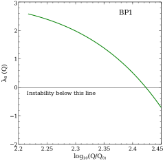
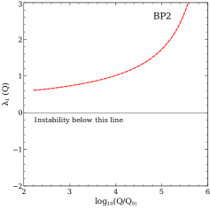
Figure 1: Running of $\lambda_{8}$ corresponding to BP1 (left) and $\lambda_{1}$ corresponding to BP2 (right). $m_{h}$ = 125 GeV and an exact alignment sin($\beta-\alpha$) = 1.0 taken in both.

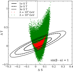
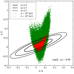
Figure 2: Contribution of the $S_{3}$HDM scalars to the oblique paramaters for sin($\beta-\alpha$) = 1.0 (Left) and sin($\beta-\alpha$) = 0.98 (Right). The ellipses denote the 1$\sigma$ (solid), 2$\sigma$ (dashed) and 3$\sigma$ (dotted) limits. The green and red points indicate validity till $10^{4}$ GeV and $10^{6}$ GeV respectively. We notice that the oblique parameters do not change appreciably for a slight departure from exact alignment.

The bounds finally obtained on $\lambda_{i}$, taking into account the oblique parameter and the diphoton constraints, are are summarised in the Table 2.

Parameter	$\Lambda=10^{3}$ GeV	$\Lambda=10^{4}$ GeV	$\Lambda=10^{6}$ GeV
$\lambda_{1}\in$	[0, 2.7]	[0, 1.4]	[0, 0.7]
$\lambda_{2}\in$	[-2.7, 2.5]	[-1.4, 1.3]	[-0.6, 0.6]
$\lambda_{3}\in$	[-2.2, 2.6]	[-1.0, 1.3]	[-0.2, 0.6]
$\lambda_{4}\in$	[-2.1, -0.1]	[-0.9, -0.1]	[-0.4, -0.1]
$\lambda_{5}\in$	[-2.7, 5.5]	[-1.1, 3.0]	[-0.4, 1.5]
$\lambda_{6}\in$	[-5.3, 4.0]	[-2.6, 1.9]	[-1.1, 0.7]
$\lambda_{7}\in$	[-2.2, 0.9]	[-1.0, 0.3]	[-0.4, 0]
$\lambda_{8}\in$	[0, 3.8]	[0, 1.9]	[0.1, 1.1]

Table 2: Bounds on the quartic couplings, for $\Lambda=10^{3},10^{4},10^{6}$ GeV. Oblique parameter and diphoton constraints are also taken into account. We show the numbers up to the first decimal place.

The $h\rightarrow\gamma\gamma$ rate diminishes with respect to the SM throughout the parameter space, however only for a strict imposition of sin($\beta-\alpha$) = 1[39]. We have projected the $S_{3}$HDM $\mu_{\gamma\gamma}$ values versus $m_{H^{+}_{1}}$ and $m_{H^{+}_{2}}$ in Fig.(3). The dimensionful $hH^{+}_{i}H^{-}_{i}$ denoted by $g_{hH^{+}_{i}H^{-}_{i}}$ is conveniently expressed through  $g_{hH^{+}_{i}H^{-}_{i}}=\frac{2\kappa_{i}m^{2}_{H^{+}_{i}}}{v}$ , where $\kappa_{i}$ are dimensionless. Whenever $\alpha=\beta-\frac{\pi}{2}$, it is seen that $\kappa_{i}=-\Big{(}1+\frac{m^{2}_{h}}{2m^{2}_{H^{+}_{i}}}\Big{)}$ [39] (exact expression given in Appendix C). A decrement in $\mu_{\gamma\gamma}$, in an exact alignment case thus becomes inevitable, since both $\kappa_{1}$ and $\kappa_{2}$ are always negative (see Appendix C). In fact, $\mu_{\gamma\gamma}$ never exceeds 0.82 for validity till $10^{6}$ GeV, given that $|\kappa_{1}|$, $|\kappa_{2}|$ $\geq$ 1.39 in that case. Following a similar trend, the points valid till $\Lambda$ = $10^{7}$ GeV give $\mu_{\gamma\gamma}$ $\textless$ 0.63 and hence are not phenomenologically acceptable. The bounds put on $\lambda_{i}$ translate into corresponding bounds on tan$\beta$ and the non-standard scalar masses, as shown in Fig.4. We point out that while $m_{H_{2}}$ could be up to 270 GeV for $\Lambda$ = $10^{6}$ GeV, the other masses do not exceed 210 GeV for most parameter points. It is to be noted that $\kappa_{1}$ and $\kappa_{2}$ can take either sign for departure from exact alignment, and hence an increment in the diphoton rate is possible there. (See Fig.(3) for sin($\beta-\alpha$) = 0.98.)

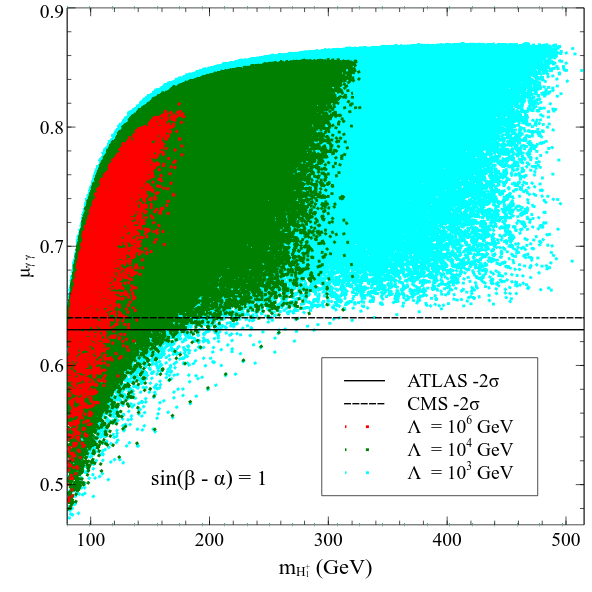
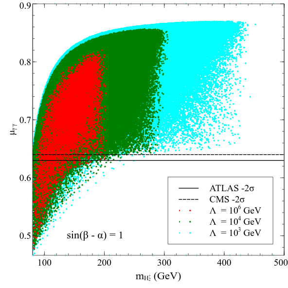
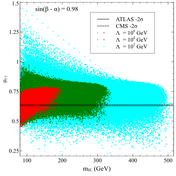
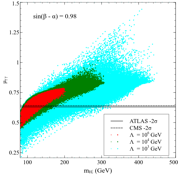
Figure 3: $h\rightarrow\gamma\gamma$ rates for an $S_{3}$HDM valid till a cut-off $\Lambda$. The cyan, green and red points are respectively for $\Lambda=10^{3},10^{4}~{}\rm and~{}10^{6}$ GeV. The solid and dotted lines denote the 2$\sigma$ limits below the central value given by ATLAS and CMS respectively .

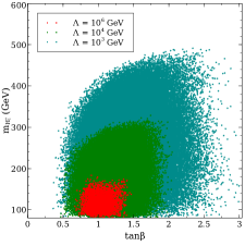
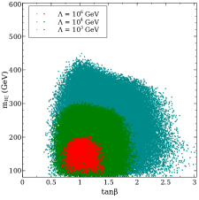
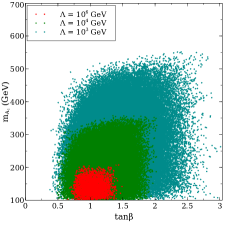
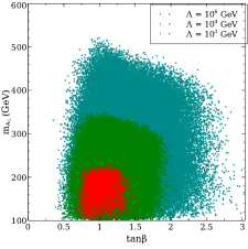
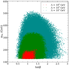
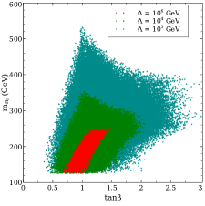
Figure 4: Regions consistent with the theoretical constraints up to a given cut-off. The cyan, green and red points are valid till $10^{3}$ GeV, $10^{4}$ GeV and $10^{6}$ GeV respectively. Oblique parameter and diphoton constraints are also taken into account. Points valid till $10^{7}$ GeV get disallowed by the diphoton constraint and are hence not displayed. An exact alignment is chosen and it has been checked that the bounds do not change for a small deviation from exact alignment.

A generic feature in context of Scenario A is that, the mass parameters $m^{2}_{11}$ and $m^{2}_{33}$ get traded off through the tadpole conditions, making $\lambda_{i}$ expressible in terms of the physical scalars only. Thus for physical scalars luking below 1TeV, $\lambda_{i}$ are already $\mathcal{O}$(1) or even larger at the input scale. This does not lead to a model that is perturbative at a high scale. As a possible remedy, additional mass parameters in the equations relating $\lambda_{i}$ to the physical masses could induce cancellations keeping the quartics further small at the EW scale. This could be achieved either through inclusion of quadratic terms violating $S_{3}$, or through invoking an inert vev structure where all of $m^{2}_{11}$ and $m^{2}_{33}$ do get not eliminated. These terms can elevate the non-standard masses to around $\sim$ 1 TeV and can also lead to $\mu_{\gamma\gamma}\textgreater$ 1. Since a broken $S_{3}$ group is beyond the ambit of the present study, we focus on the inert case (Scenario B) in the subsequent section.

4.2 Scenario B: $v_{1}$ = $v_{2}$ = 0, $v_{3}$ = 246 GeV.

One needs to put $\lambda_{4}$ = 0 in order to keep the DM stable through an unbroken $Z_{2}$ symmetry. Correct relic density is obtained in the mass regimes $m_{H_{1}}\textless~{}\rm~{}80~{}GeV$ and $m_{H_{1}}\textgreater~{}\rm 370~{}GeV$. We discuss below the phenomenology in detail.

4.2.1 $m_{H_{1}}\textless~{}\rm 80~{}GeV$.

DM particles dominantly annihilate to the $b\bar{b}$ final state through an $h$ in the s-channel, in this mass regime. A sharp decline in relic abundance is noted for $m_{H_{1}}\textgreater~{}\rm 80~{}GeV$, when the $VV$ ($V$ denoting a vector boson.) mode opens up. Maintaining appropriate mass gaps amongst $H_{1}$, $A_{1}$ and $H^{+}_{1}$ turns advantageous in the two following ways. Firstly, the DM relic abundance does not deplete fast through co-annihilations brought in by by a narrow mass splitting. Secondly, it gives sizable values to $\lambda_{5}$, $\lambda_{6}$ and $\lambda_{7}$ which in turn aid to stabilize the vacuum far beyond the SM instability scale, even up to the Planck scale. Overall, the phenomenology in this mass regime is broadly similar to the case with a single inert doublet.

Benchmark	$m_{H_{1}}$(GeV)	$m_{A_{1}}$(GeV)	$m_{H^{+}_{1}}$(GeV)	$\lambda_{L}$	$\Omega h^{2}$	$\sigma_{SI}(cm^{2})$	$\Lambda$(GeV)
BP3	57.00	102.00	120.00	0.0042	0.1170	$4.63\times 10^{-47}$	$10^{19}$

Table 3: Benchmark point illustrating the behaviour under RGE. $\Lambda$ denotes the maximum extrapolation scale up to which vacuum stability and perturbativity are ensured.

The displayed benchmark BP3 (Table 3) keeps BR($h\rightarrow\rm invisible$) $\textless$ 19 $\%$ owing to the tiny $\lambda_{L}$. A perturbative theory at high scales requires $m_{A_{1}}$ and $m_{H^{+}_{1}}$ to obey sharp upper bounds, a feature not reflected by the DM constraints alone. For instance, we need $m_{A_{1}}$, $m_{H^{+}_{1}}$ $\textless$ 135 GeV in order to salvage perturbativity till the GUT scale.

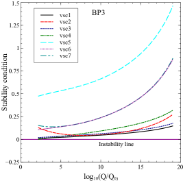
Figure 5: Evolution of BP3 under RG. Colour coding is explained in the legends and the vacuum instability line is highlighted.

4.2.2 $m_{H_{1}}\textgreater~{}\rm 370~{}GeV$.

In this region, dark matter relic density tends to diminish due to prohibitively large annihilation to $VV$ final states. Annihilations in this case are the interference of $H_{1}-H_{1}-V-V$ four-point coupling and the $t/u$ channel diagrams with $H^{+}_{1}/A_{1}$ in the propagator. However, a small splitting among the masses of the inert scalars induces cancellation between these two classes of diagrams thereby burgeoning relic density to the desired range. Larger is $m_{H_{1}}$, higher is the annihilation to the longitudinal gauge bosons and hence higher becomes $\lambda_{L}$. While a similar phenomenology occurs in case of a single inert doublet, apart from the DM mass $\textless$ 80 GeV region, $\Omega h^{2}$ is $\sim$ 0.1 again only when the DM mass $\textgreater$ 500 GeV. For example, for $m_{H_{1}}$ = 387.5, $m_{A_{1}}$ = 390.5, $m_{H^{+}_{1}}$ = 389.6, $\lambda_{L}$ = 0.056, the dominant annihilation channels are $H_{1}H_{1}$ $\rightarrow$ $WW$ 12$\%$, $H_{2}H_{2}$ $\rightarrow$ $WW$ 12$\%$, $H_{1}H_{1}$ $\rightarrow$ $ZZ$ 10$\%$, $H_{2}H_{2}$ $\rightarrow$ $ZZ$ 10$\%$, $H^{+}_{1}H^{-}_{1}$ $\rightarrow$ $WW$ 6$\%$, $H^{+}_{2}H^{-}_{2}$ $\rightarrow$ $WW$ 6$\%$, $H^{+}_{1}H_{1}$ $\rightarrow$ $\gamma W^{+}$ 6$\%$, $H^{+}_{2}H_{2}$ $\rightarrow$ $\gamma W^{+}$ 6$\%$. For a spectrum $m_{H_{1}}$ = 904.1, $m_{A_{1}}$ = 912.1, $m_{H^{+}_{1}}$ = 904.3, the requisite $\lambda_{L}$ for a correct relic increases to $\sim$ 0.49. One thus requires a small mass splitting and an appropriately adjusted $\lambda_{L}$ to generate correct relic density.

To examine high-scale validity of this scenario, model points are generated in the following range.

$$\lambda_{L}\in[-4\pi,4\pi]$$ (4.1)

$$m_{H_{1}}\in[300.0~{}\rm GeV,1000.0~{}\rm GeV]$$ (4.2)

$$m_{A_{1}}\in[m_{H_{1}},m_{H_{1}}+100.0~{}\rm GeV]$$ (4.3)

$$m_{H^{+}_{1}}\in[m_{H_{1}},m_{H_{1}}+100.0~{}\rm GeV]$$ (4.4)

We also fix $\lambda_{1}$ = $\lambda_{2}$ = $\lambda_{3}$ = 0.01 at the initial scale, since these couplings do not enter into the calculations of relic density and WIMP-nucleon cross sections. This choice is rather judicious, an higher value mostly makes the couplings non-perturbative at high scales. Fig.6 displays the variation of relic density corresponding to model points valid up to three different cut-offs $\Lambda=10^{3}$ GeV, $10^{16}$ GeV and $10^{19}$ GeV. Fig.7 projects spin-independent WIMP-nucleon cross section.

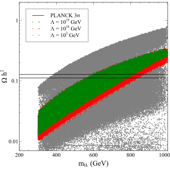
(a)

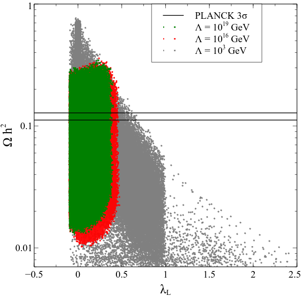
(b)

Figure 6: The dark matter relic density versus $m_{H_{1}}$ (left) and the coupling of $H_{1}$ pair to the Higgs boson $\lambda_{L}$ (right). The grey, green and red points preserve validity up to 1TeV, the GUT scale $10^{16}$ GeV and the Planck scale $10^{19}$ GeV respectively. The horizontal black lines denote the 3$\sigma$ limits of the PLANCK data. .

An inspection of Fig.6 and Fig.7 points out that one can render the $S_{3}$HDM stable upto GUT and Planck scales with initial conditions consistent with the observations of relic density and direct detection. We highlight this fact as the most important conclusion in this part. This, however happens only if $m_{H_{1}}\textgreater$ 550 GeV. This result be understood as follows. The evolution of $\lambda_{8}$ and hence vacuum stability is crucially dictated by the values of $\lambda_{5}$, $\lambda_{6}$ and $\lambda_{7}$ at the initial scale. They can be expressed in terms of the masses as,

$$\lambda_{5} = \lambda_{L}+\frac{2}{v^{2}}(m_{H^{+}_{1}}^{2}-m_{H_{1}}^{2})$$ (4.5)

$$\lambda_{6} = \frac{1}{v^{2}}(m_{H_{1}}^{2}+m_{A_{1}}^{2}-2m_{H^{+}_{1}}^{2})$$ (4.6)

$$\lambda_{7} = \frac{1}{2v^{2}}(m_{H_{1}}^{2}-m_{A_{1}}^{2})$$ (4.7)

We find that for an $H_{1}$ below 600 GeV, $\lambda_{5}$, $\lambda_{6}$ and $\lambda_{7}$ are not sizable enough to ensure $\lambda_{8}(Q)\textgreater 0$ up to the GUT scale. On the other hand, perturbative unitarity restricts the mass splitting to $\sim$ 50 GeV which is automatically consistent with the $T$ parameter constraint. While the stability condition $\lambda_{5}+2\sqrt{\lambda_{8}(\lambda_{1}+\lambda_{3})}~{}\textgreater~{}0$ disfavours large negative values of $\lambda_{5}$, tight upper bounds are imposed by perturbative unitarity. This translates into $-0.1\textless\lambda_{L}\textless 0.4$ for a model valid up to $M_{Pl}$ (see Fig.6).

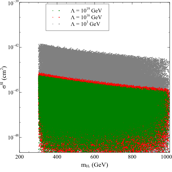
(a)

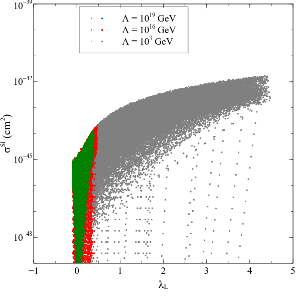
(b)

Figure 7: Spin independent WIMP-nucleon scattering cross section vs $m_{H_{1}}$ (left) and the coupling of $H_{1}$ pair to the Higgs boson $\lambda_{L}$ (right). The grey, green and red points preserve validity up to 1TeV, the GUT scale $10^{16}$ GeV and the Planck scale $10^{19}$ GeV respectively. Note that a large proportion of model points do obey the LUX upper bound while fulfilling stability requirements.

For a more comprehensive understanding, the parameter space negotiating all the imposed constraints successfully is displayed as correlation plots in Fig.8. Our demand of $\sigma^{\rm SI}\textless 10^{-46}$ $\rm cm^{2}$ throughout in Fig.8 automatically complies with the LUX results. The DM masses are strongly restricted by the requirements of DM searches, and high-scale validity till a given $\Lambda$. For instance we note $m_{H_{1}}\in$ [550 GeV, 830 GeV] and [550 GeV, 750 GeV] for $\Lambda$ = $M_{\rm GUT}$ and $\Lambda$ = $M_{Pl}$ respectively (see Fig.8).

(a)

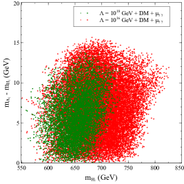
(b)

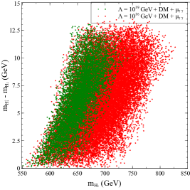
(c)

Figure 8: The viable $S_{3}$HDM parameter space projected on the $\lambda_{L}$ vs $m_{H_{1}}$ (top left), $m_{A_{1}}-m_{H_{1}}$ vs $m_{H_{1}}$ (top right), $m_{H^{+}_{1}}-m_{H_{1}}$ vs $m_{H_{1}}$ (bottom) planes. ”$\Lambda$ + DM + $\mu_{\gamma\gamma}$” in the legends refers to validity up to $\Lambda$ as well as consistency with DM searches and diphoton signal strength. The green and red points correspond to $\Lambda=10^{16}$ GeV and $\Lambda=10^{19}$ GeV respectively.

A situation, where $\mu_{\gamma\gamma}\textless 1$ (Fig.9) for most part of the parameter space is attributed to a mostly non-negative $\lambda_{5}$ (or a very small negative value). The reader should note that unlike the previous case, one can in principle have $\mu_{\gamma\gamma}\textgreater 1$ in this case, however subject to stability constraints. With $\lambda_{1}=\lambda_{3}=0.01$ at the input scale, $\lambda_{5}$ gets bounded from below at $\simeq$ -0.1 by the vacuum stability condition $\lambda_{5}\textgreater-2\sqrt{\lambda_{8}(\lambda_{1}+\lambda_{3})}$.

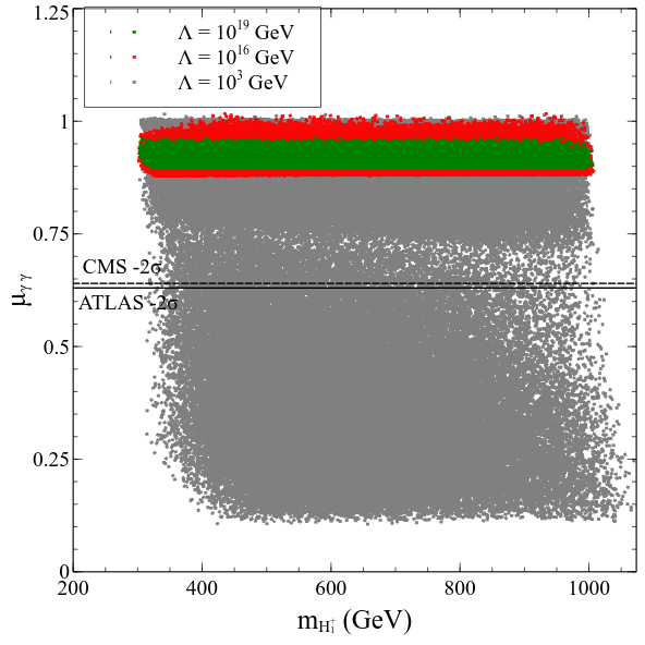
(a)

Figure 9: Distribution of parameter points valid till $10^{3}$ GeV (grey), $10^{16}$ (red) GeV and $10^{19}$ (green) GeV in the $\mu_{\gamma\gamma}$ vs $m_{H^{+}_{1}}$ plane. The solid and dotted lines denote the 2$\sigma$ limits below the central value given by ATLAS and CMS respectively .

One can get a deeper lower bound, and hence a $\mu_{\gamma\gamma}$ substantially larger than unity for larger values of $\lambda_{1}$ and $\lambda_{3}$, but in that case one does not have a perturabtive theory till $10^{19}$ GeV. Very low values of $\mu_{\gamma\gamma}$ seen in Fig.9 are possible for points valid only up to the TeV scale, where a positive $\lambda_{5}$ as large as $\sim$ 6.5 is allowed without causing a breakdown of perturbativity below 1TeV. Parameter points valid till the GUT and Planck scales rarely correspond a diphoton signal strength less than 0.87. This indeed is within the 2$\sigma$ limit from both the ATLAS and CMS central values. This very observation that validity till very high scales always predicts a depletion in the diphoton rate, but still can be kept within the experimental bounds emerges as an important consequence in this regard. The diphoton rate thus bears fingerprints of an extended Higgs sector such as the $S_{3}$HDM, whose tree level couplings could mimic the corresponding SM ones. This calls for its accurate measurements in 13 TeV LHC for instance, or at the other upcoming colliders.

To sum up, DM phenomenology plays a vital role in deciding the fate of this scenario at high scales. The interplay of various effects involved is captured through the benchmarks in Table 4. The RG running of these benchmarks is shown in Fig.10 The first benchmark BP4 can possibly describe physics nearly up to the GUT scale, beyond which perturbativity breaks down. However, BP4 predicts a relic density below the observed limit. This is attributed to the relatively large mass splittings amongst the $S_{3}$ scalars, which generate such sizable $\lambda_{5}$, $\lambda_{6}$ and $\lambda_{7}$ at the initial scale that can ensure $\lambda_{8}$(Q) $\textgreater$ 0 throughout. However we pay the price of a diminished co-annihilation, and thereby a relic density below the desired range. A fall out of this relatively large $\lambda_{5}$ in this case is a suppressed $\mu_{\gamma\gamma}$. BP5 highlights the fact that correct relic density and direct detection rates are achievable in this model for a DM around 390 GeV, a feature not observed in the model with a single inert doublet. The maximal mass difference in such a case is restricted to $\sim$ 13 GeV. However, BP5 does not keep the EW vacuum stable beyond $10^{8}$ GeV.

Benchmark	$m_{H_{1}}$(GeV)	$m_{A_{1}}$(GeV)	$m_{H^{+}_{1}}$(GeV)	$\lambda_{L}$	$\Omega h^{2}$	$\sigma_{SI}(cm^{2})$	$\Lambda$(GeV)
BP4	479.200	480.475	494.525	-0.0236	0.0635	2.13 $\times$ $10^{-47}$	$10^{19}$
BP5	390.000	391.000	392.000	0.0050	0.1200	1.44 $\times$ $10^{-48}$	$10^{8}$
BP6	707.400	720.000	713.500	0.032	0.1214	1.80 $\times$ $10^{-47}$	Just below $10^{16}$
BP7	718.600	727.450	727.225	0.0268	0.1263	1.22 $\times$ $10^{-47}$	$10^{19}$

Table 4: Benchmark points chosen to illustrate the behaviour under RGE. $\Lambda$ denotes the maximum extrapolation scale up to which vacuum stability and perturbativity are ensured.

BP6 and BP7 are conservative choices which predict relic density and direct-detection rates in the correct ballpark, and also extrapolate the model to the GUT and Planck scales respectively. We note here that in BP4, BP6 and BP7, vsc1, vsc3, vsc4, vsc5, vsc6, vsc7 rise with $Q$, whereas in BP5, vsc5 and vsc6 go down. This observation has its root in the structure of the $S_{3}$HDM beta functions (see Appendix.A), which mostly guarantee vsc1, vsc3, vsc4, vsc5, vsc6, vsc7 $\textgreater$ 0 throughout the evolution once they start with positive values at the EW scale. We remark here that BP6 and BP7 correspond to $\mu_{\gamma\gamma}$ = 0.935 and 0.911 respectively,which are within the 2$\sigma$ limit from the central value.

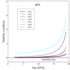
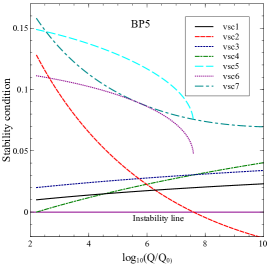
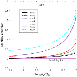
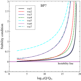
Figure 10: RG Evolution of BP4, BP5, BP6 and BP7. Colour coding is explained in the legends and the vacuum instability line is highlighted. Note that vsc5 and vsc6 are not defined whenever $\lambda_{8}$ $\textless$ 0.

In the same connection, we have found that an $m_{H_{1}}\textgreater$ 1 TeV can render the EW vacuum stable at least up to the SM instability scale. However that pushes $\mu_{11}$ to yet higher values, thereby introducing a so-called intermediate scale into the picture. It is then implied that the $S_{3}$ scalars are practically decoupled below $\mu_{11}$, and that it would be more appropriate to solve the RG equations in a piecewise fashion, i.e., evolve from the EW scale to $\mu_{11}$ using the SM beta functions only, and then invoke $S_{3}$HDM above the $\mu_{11}$ threshold. However we mostly encounter $\mu_{11}$ $\lesssim$ 600 GeV for $S_{3}$ masses $\textless$ 1 TeV. We have checked that for such a $\mu_{11}$, a piecewise evolution practically gives the same numerical results.

5 Conclusions and future work

3HDMs offer a rich scalar spectrum and can give rise to prominent signatures at the colliders[21, 22]. In this paper, we have tried to investigate an $S_{3}$-symmetric Higgs sector in the light of various theoretical as well as experimental constraints. Robust regimes of the model parameter space were surveyed using the latest data on the 125 GeV Higgs and oblique parameters. The high-scale behaviour was probed by evolving the model couplings under the RGEs, and this study appears to be the first attempt in that direction in context of 3HDMs. A unitary and perturbative theory, along with a stable EW vacuum was ensured at each step of evolution. We have illustrated our findings in context of two specific alignment of the doublet vevs. The salient features of the numerical results that emerge are highlighted below.

• In the first case, non-zero vevs are assigned to all three of the doublets while maintaining $v_{1}=\surd 3v_{2}$. It is found that this scenario is not stable beyond $10^{7}$ GeV, an effect brought about by an interplay of perturbative unitarity and vacuum stability. Stringent upper bounds are placed on the scalar masses and tan$\beta$ in this case. In particular we note tan$\beta$ $\textless$ 1.3 and the $S_{3}$ scalar masses lie below 270 GeV for $\Lambda$ = $10^{6}$ GeV, the maximum phenomenologically accepted scale.

• The second case is a scenario with two inert doublets. There lies an identifiable region in the parameter space in this case that extends validity of the model till the Planck scale. Moreover, this parameter space is robust enough to accomodate a successful canditate for dark matter. High-scale stability in this case manifests itself by placing upper bounds on the coupling of the DM to the 125 GeV Higgs, the DM mass, as well on the mass splitting amongst the inert scalars. The bounds get sharper when both the DM as well as high-scale stability constraints are imposed simultaneously. In a word, a connection emerges between DM phenomenology at the low scale and a good UV behaviour at high scales. This finding is qualitatively similar to the model with a single inert doublet[9]. However, the addition of the extra inert doublet narrows down the gap between the low and high DM mass regions, with respect to what is observed in the single inert doublet case.

• Scenario B predicts a decrement in the diphoton decay width with respect to the SM value, so does Scenario A for an exact alignment. This particular feature of Scenario B is not seen by considering tree-level stability constraints alone and is an explicit consequence of renormalisation group evolution. The numerical predictions however can be made to lie within the current experimental limits without running into conflict with high-scale stability.

Altogether then, we conclude that the inert scenario fares much better than the non-inert one in terms of high-scale validity and signal strength measurements. It is thus safe to comment that the $S_{3}$HDM can certainly alleviate the vacuum stability problem, however not for all permissible vev structures. Several extensions of the present study are possible. One could analyze a more general $S_{3}$-symmetric Yukawa texture in a similar context, admittedly though such texture would give rise to Flavor-Changing Neutral Currents (FCNC)[32] at the tree level. It was shown in [63] that raising the $S_{3}$ masses to $\sim$10 TeV suppresses the possible FCNCs. The requirement of such heavy scalars necessiates the inclusion of $S_{3}$ violating quadratic terms[24]. Another motivation of a broken $S_{3}$ symmetry is in the context of DM. In scenario B for instance, it will lead to a non-degenrate spectrum and hence a modified DM phenomenology, at least at the quantitative level. Indirect detection signatures of such a DM scenario could be of special importance in light of latest data. Adding further to it, the large number of bosonic degrees of freedom offered by the $S_{3}$HDM could favour a strong first order electroweak phase transition, thereby making way for baryogenesis, something already looked at for a more generic 3HDM with two inert doublets. [64].

6 Acknowledgements

I thank Aritra Gupta for useful discussions, Arijit Dutta for a computational aid, and Biswarup Mukhopadhyaya for his insightful comments on the manuscript. I also acknowledge the funding available from the Department of Atomic Energy, Government of India, for the Regional Centre for Accelerator based Particle Physics (RECAPP), Harish-Chandra Research Institute.

Appendix.

Appendix A Renormalisation group (RG) equations

We list the one-loop RG equations for the model couplings used throughout the analysis. For the gauge couplings, they are given by [65],

$$16\pi^{2}\frac{dg_{s}}{dt} = -7g_{s}^{3},$$ (A.1a)

$$16\pi^{2}\frac{dg}{dt} = -\frac{17}{6}g^{3},$$ (A.1b)

$$16\pi^{2}\frac{dg^{\prime}}{dt} = \frac{43}{6}{g^{\prime}}^{3}.$$ (A.1c)

The quartic couplings evolve according to,

$$16\pi^{2}\beta_{\lambda_{1}} = 32\lambda_{1}^{2}+8\lambda_{2}^{2}+16\lambda_{3}^{2}+4\lambda_{4}^{2}+2\lambda_{5}^{2}+\frac{1}{2}\lambda_{6}^{2}-8\lambda_{1}\lambda_{2}+16\lambda_{1}\lambda_{3}$$ (A.2a)

$$+2\lambda_{5}\lambda_{6}+2\lambda_{7}^{2}+\frac{3}{8}(g^{\prime 4}+3g^{4})-\lambda_{1}(9g^{2}+3g^{\prime 2})\$$

$$16\pi^{2}\beta_{\lambda_{2}} = 24\lambda_{1}\lambda_{2}-24\lambda_{2}^{2}-16\lambda_{2}\lambda_{3}-\frac{1}{2}\lambda_{6}^{2}+2\lambda_{7}^{2}-\frac{3}{4}g^{\prime 2}g^{2}$$ (A.2b)

$$-\lambda_{2}(9g^{2}+3g^{\prime 2})\$$

$$16\pi^{2}\beta_{\lambda_{3}} = 16\lambda_{3}^{2}+8\lambda_{4}^{2}+24\lambda_{1}\lambda_{3}+8\lambda_{2}\lambda_{3}+8\lambda_{4}^{2}+\frac{1}{2}\lambda_{6}^{2}+2\lambda_{7}^{2}+\frac{3}{4}g^{\prime 2}g^{2}$$ (A.2c)

$$-\lambda_{3}(9g^{2}+3g^{\prime 2})\$$

$$16\pi^{2}\beta_{\lambda_{4}} = \lambda_{4}(12\lambda_{1}+4\lambda_{2}+24\lambda_{3}+6\lambda_{5}+8\lambda_{6}+20\lambda_{7})$$ (A.2d)

$$-\lambda_{4}(9g^{2}+3g^{\prime 2}-3y_{t}^{2})\,,$$

$$16\pi^{2}\beta_{\lambda_{5}} = 4\lambda_{5}^{2}+2\lambda_{6}^{2}+8\lambda_{4}^{2}+8\lambda_{7}^{2}+20\lambda_{1}\lambda_{5}-4\lambda_{2}\lambda_{5}+8\lambda_{3}\lambda_{5}+8\lambda_{1}\lambda_{6}$$ (A.2e)

$$+12\lambda_{5}\lambda_{8}+4\lambda_{6}\lambda_{8}+\frac{3}{4}(g^{\prime 4}-2g^{\prime 2}g^{2}+3g^{4})-\lambda_{5}(9g^{2}+3g^{\prime 2}-6y_{t}^{2})\,,$$

$$16\pi^{2}\beta_{\lambda_{6}} = 20\lambda_{4}^{2}+4\lambda_{6}^{2}+32\lambda_{7}^{2}+4\lambda_{1}\lambda_{6}-4\lambda_{2}\lambda_{6}+8\lambda_{3}\lambda_{6}+8\lambda_{5}\lambda_{6}+4\lambda_{8}\lambda_{6}+3g^{\prime 2}g^{2}$$ (A.2f)

$$-\lambda_{6}(9g^{2}+3g^{\prime 2}-6y_{t}^{2})\,,$$

$$16\pi^{2}\beta_{\lambda_{7}} = 4\lambda_{7}(\lambda_{1}+\lambda_{2}+2\lambda_{3}+2\lambda_{5}+3\lambda_{6}+\lambda_{8})+10\lambda_{4}^{2}$$ (A.2g)

$$-\ \lambda_{7}(9g^{2}+3g^{\prime 2}-6y_{t}^{2})\,,$$

$$16\pi^{2}\beta_{\lambda_{8}} = 4\lambda_{5}^{2}+4\lambda_{5}\lambda_{6}+2\lambda_{6}^{2}+8\lambda_{7}^{2}+24\lambda_{8}^{2}+\frac{3}{8}(g^{\prime 4}+2g^{\prime 2}g^{2}+3g^{4})$$ (A.2h)

$$-\ \lambda_{8}(9g^{2}+3g^{\prime 2}-12y_{t}^{2})-6y_{t}^{4}\,,$$

Neglecting the effect of other quarks, the t-quark Yukawa coupling has the beta function,

$$16\pi^{2}\beta_{y_{t}} = y_{t}\left(-8g_{s}^{2}-\frac{9}{4}g^{2}-\frac{17}{12}g^{\prime 2}+\frac{9}{2}y_{t}^{2}\right)\,$$ (A.3)

Appendix B Oblique parameters

The expressions for the oblique parameters in the $S_{3}$HDM are given. A shorthand notation sin$(\beta-\alpha)$ = $s_{\beta-\alpha}$, cos$(\beta-\alpha)$ = $c_{\beta-\alpha}$ is adopted,

$$\Delta S = (2s_{W}^{2}-1)^{2}G(m_{H^{+}_{1}}^{2},m_{H^{+}_{1}}^{2},m_{Z}^{2})+(2s_{W}^{2}-1)^{2}G(m_{H^{+}_{2}}^{2},m_{H^{+}_{2}}^{2},m_{Z}^{2})+G(m_{H_{2}}^{2},m_{A_{1}}^{2},m_{Z}^{2})$$ (B.1a)

$$+c_{\beta-\alpha}^{2}G(m_{h}^{2},m_{A_{2}}^{2},m_{Z}^{2})+s_{\beta-\alpha}^{2}G(m_{H_{1}}^{2},m_{A_{2}}^{2},m_{Z}^{2})+c_{\beta-\alpha}^{2}G(m_{H_{1}}^{2},m_{H_{1}}^{2},m_{Z}^{2})$$

$$-s_{\beta-\alpha}^{2}G(m_{h}^{2},m_{h}^{2},m_{Z}^{2})-2{ln(m_{H^{+}_{1}}^{2})}-2ln(m_{H^{+}_{2}}^{2})+ln(m_{H_{2}}^{2})+ln(m_{H_{1}}^{2})+ln(m_{A_{1}}^{2})$$

$$+ln(m_{A_{2}}^{2})$$

$$\Delta T = F(m_{H^{+}_{1}}^{2},m_{H_{2}}^{2})+F(m_{H^{+}_{1}}^{2},m_{A_{1}}^{2})+c_{\beta-\alpha}^{2}F(m_{H^{+}_{2}}^{2},m_{h}^{2})+s_{\beta-\alpha}^{2}F(m_{H^{+}_{2}}^{2},m_{H_{1}}^{2})-F(m_{H_{2}}^{2},m_{A_{1}}^{2})$$ (B.1b)

$$-c_{\beta-\alpha}^{2}F(m_{h}^{2},m_{A_{2}}^{2})-s_{\beta-\alpha}^{2}F(m_{H_{1}}^{2},m_{A_{2}}^{2})+3c_{\beta-\alpha}^{2}(F(m_{Z}^{2},m_{H_{1}}^{2})-F(m_{W}^{2},m_{H_{1}}^{2}))$$

$$-3c_{\beta-\alpha}^{2}(F(m_{Z}^{2},m_{h}^{2})-F(m_{W}^{2},m_{h}^{2}))$$

$$\Delta U = \frac{1}{24\pi}[G(m_{H^{+}_{1}}^{2},m_{H_{2}}^{2},m_{W}^{2})+G(m_{H^{+}_{1}}^{2},m_{A_{1}}^{2},m_{W}^{2})+c_{\beta-\alpha}^{2}G(m_{H^{+}_{2}}^{2},m_{h}^{2},m_{W}^{2})$$ (B.1c)

$$+s_{\beta-\alpha}^{2}G(m_{H^{+}_{2}}^{2},m_{H_{1}}^{2},m_{W}^{2})+G(m_{H^{+}_{2}}^{2},m_{A_{2}}^{2},m_{W}^{2})+c_{\beta-\alpha}^{2}\hat{G}(m_{H_{1}}^{2},m_{W}^{2})-\hat{G}(m_{H_{1}}^{2},m_{Z}^{2})$$

$$-c_{\beta-\alpha}^{2}\hat{G}(m_{h}^{2},m_{W}^{2})-\hat{G}(m_{h}^{2},m_{Z}^{2})-G(m_{H_{2}}^{2},m_{A_{1}}^{2},m_{Z}^{2})-c_{\beta-\alpha}^{2}G(m_{h}^{2},m_{A_{2}}^{2},m_{Z}^{2})$$

$$-s_{\beta-\alpha}^{2}G(m_{H_{1}}^{2},m_{A_{2}}^{2},m_{Z}^{2})-(2s_{W}^{2}-1)^{2}G(m_{H^{+}_{1}}^{2},m_{H^{+}_{1}}^{2},m_{Z}^{2})$$

$$-(2s_{W}^{2}-1)^{2}G(m_{H^{+}_{2}}^{2},m_{H^{+}_{2}}^{2},m_{Z}^{2})]$$

where,

$$F\left(m_{1}^{2},m_{2}^{2}\right)\equiv\left\{\begin{array}[]{lcl}\displaystyle{\frac{m_{1}^{2}+m_{2}^{2}}{2}-\frac{m_{1}^{2}m_{2}^{2}}{m_{1}^{2}-m_{2}^{2}}\,\ln{\frac{m_{1}^{2}}{m_{2}^{2}}}}&;&m_{1}^{2}\neq m_{2}^{2},\\[8.53581pt] 0&;&m_{1}^{2}=m_{2}^{2}.\end{array}\right.$$ (B.2)

$$G\left(m_{1}^{2},m_{2}^{2},q^{2}\right) \equiv -\frac{16}{3}+\frac{5\left(m_{1}^{2}+m_{2}^{2}\right)}{q^{2}}-\frac{2\left(m_{1}^{2}-m_{2}^{2}\right)^{2}}{(q^{2})^{2}}$$ (B.3)

$$+\frac{3}{q^{2}}\left[\frac{m_{1}^{4}+m_{2}^{4}}{m_{1}^{2}-m_{2}^{2}}-\frac{m_{1}^{4}-m_{2}^{4}}{q^{2}}+\frac{\left(m_{1}^{2}-m_{1}^{2}\right)^{3}}{3q^{4}}\right]\ln{\frac{m_{1}^{2}}{m_{2}^{2}}}+\frac{r}{(q^{2})^{3}}\,f\left(t,r\right)~{}~{}~{}~{}~{}~{}~{}~{}~{}$$

$$\tilde{G}\left(m_{1}^{2},m_{2}^{2},q^{2}\right)\equiv-2+\left(\frac{m_{1}^{2}-m_{2}^{2}}{q^{2}}-\frac{m_{1}^{2}+m_{2}^{2}}{m_{1}^{2}-m_{2}^{2}}\right)\ln{\frac{m_{1}^{2}}{m_{2}^{2}}}+\frac{f\left(t,r\right)}{q^{2}}.$$ (B.4)

$$\hat{G}\left(m^{2},q^{2}\right)\equiv G\left(m^{2},m^{2},q^{2}\right)+12~{}\tilde{G}\left(m^{2},m^{2},q^{2}\right)$$ (B.5)

$$t\equiv m_{1}^{2}+m_{2}^{2}-q^{2}\quad\mbox{and}\quad r\equiv(q^{2})^{2}-2q^{2}\left(m_{1}^{2}+m_{2}^{2}\right)+\left(m_{1}^{2}-m_{2}^{2}\right)^{2}$$ (B.6)

$$f\left(t,r\right)\equiv\left\{\begin{array}[]{lcl}{\displaystyle\sqrt{r}\,\ln{\left|\frac{t-\sqrt{r}}{t+\sqrt{r}}\right|}}&;&r>0,\\[8.53581pt] 0&;&r=0,\\[5.69054pt] {\displaystyle 2\,\sqrt{-r}\,\tan^{-1}{\frac{\sqrt{-r}}{t}}}&;&r<0.\end{array}\right.$$ (B.7)

These are standard functions arising in a one-loop calculation.

Appendix C $h\rightarrow\gamma\gamma$ decay width

The partial decay width of the SM-like Higgs to a pair of photons in this case has the expression[66],

$$\Gamma(h\to\gamma\gamma)=\frac{\alpha^{2}g^{2}}{2^{10}\pi^{3}}\frac{m_{h}^{3}}{M_{W}^{2}}\Big{|}sin(\beta-\alpha)F_{W}+\Big{(}-\frac{sin\alpha}{cos\beta}\Big{)}\frac{4}{3}F_{t}+\sum_{i=1}^{2}\kappa_{i}F_{i+}\Big{|}^{2}\,,$$ (C.1)

The functions ${F}_{W}$, ${F}_{t}$ and ${F}_{i+}$ capture the effects of a W-boson, a t-quark and a charged scalar running in the loop and shall be defined as,

$$F_{W} = 2+3\tau_{W}+3\tau_{W}(2-\tau_{W})f(\tau_{W})\,,$$ (C.2a)

$$F_{t} = -2\tau_{t}\big{[}1+(1-\tau_{t})f(\tau_{t})\big{]}\,,$$ (C.2b)

$$F_{i+} = -\tau_{i+}\big{[}1-\tau_{i+}f(\tau_{i+})\big{]}\,.$$ (C.2c)

$$f(\tau) = \left[\sin^{-1}\left(\sqrt{1/\tau}\right)\right]^{2}\,.$$ (C.3)

$$\rm with,~{}\tau = \frac{4m^{2}_{a}}{m^{2}_{h}}$$ (C.4)

Here, $a$ = $t$, $W$ and $H^{+}_{i}$.

For Scenario A:

$$\kappa_{1} = -\frac{1}{6v}(2\cos\alpha\ \textrm{cosec}\beta(-6m^{2}_{H_{1}}+3m^{2}_{H_{2}}-3m^{2}_{h}+m^{2}_{H_{2}}+3m^{2}_{H^{+}_{2}}\cos 2\beta)+$$ (C.5a)

$$(6m^{2}_{H^{+}_{2}}+2m^{2}_{H_{2}}+m^{2}_{H^{+}_{2}}\rm cos2\beta)\rm sec\beta~{}\rm sin\alpha)\,,$$

$$\kappa_{2} = \frac{1}{9v}((9(-2m^{2}_{H^{+}_{2}}+m^{2}_{h})\cos\beta-9m^{2}_{h}\textrm{sec}\beta+m^{2}_{H_{2}}\rm sec^{3}\beta)\sin\alpha+$$ (C.5b)

$$((9m^{2}_{h}+m^{2}_{H_{2}})\textrm{cosec}\beta+18m^{2}_{H^{+}_{2}}\sin\beta-9m^{2}_{h}\sin\beta+m^{2}_{H_{2}}\textrm{sec}\beta\tan\beta)\cos\alpha)$$

For Scenario B:

$$\kappa_{1} = \kappa_{2}=-\frac{\lambda_{5}}{2}\,.$$ (C.6a)

References

- [1] ATLAS Collaboration, G. Aad et al., Observation of a new particle in the search for the Standard Model Higgs boson with the ATLAS detector at the LHC, Phys.Lett. B716 (2012) 1–29, [arXiv:1207.7214].
- [2] CMS Collaboration, S. Chatrchyan et al., Observation of a new boson at a mass of 125 GeV with the CMS experiment at the LHC, Phys.Lett. B716 (2012) 30–61, [arXiv:1207.7235].
- [3] A. Freitas and P. Schwaller, Higgs CP Properties From Early LHC Data, Phys. Rev. D87 (2013), no. 5 055014, [arXiv:1211.1980].
- [4] A. Djouadi, R. M. Godbole, B. Mellado, and K. Mohan, Probing the spin-parity of the Higgs boson via jet kinematics in vector boson fusion, Phys. Lett. B723 (2013) 307–313, [arXiv:1301.4965].
- [5] A. Djouadi and G. Moreau, The couplings of the Higgs boson and its CP properties from fits of the signal strengths and their ratios at the 7+8 TeV LHC, Eur. Phys. J. C73 (2013), no. 9 2512, [arXiv:1303.6591].
- [6] G. Degrassi, S. Di Vita, J. Elias-Miro, J. R. Espinosa, G. F. Giudice, G. Isidori, and A. Strumia, Higgs mass and vacuum stability in the Standard Model at NNLO, JHEP 08 (2012) 098, [arXiv:1205.6497].
- [7] D. Buttazzo, G. Degrassi, P. P. Giardino, G. F. Giudice, F. Sala, A. Salvio, and A. Strumia, Investigating the near-criticality of the Higgs boson, JHEP 12 (2013) 089, [arXiv:1307.3536].
- [8] G. Bertone, D. Hooper, and J. Silk, Particle dark matter: Evidence, candidates and constraints, Phys. Rept. 405 (2005) 279–390, [hep-ph/0404175].
- [9] A. Goudelis, B. Herrmann, and O. Stål, Dark matter in the Inert Doublet Model after the discovery of a Higgs-like boson at the LHC, JHEP 09 (2013) 106, [arXiv:1303.3010].
- [10] A. Aranda, C. Bonilla, and J. L. Diaz-Cruz, Three generations of Higgses and the cyclic groups, Phys. Lett. B717 (2012) 248–251, [arXiv:1204.5558].
- [11] I. de Medeiros Varzielas, O. Fischer, and V. Maurer, symmetry at colliders and in the universe, JHEP 08 (2015) 080, [arXiv:1504.03955].
- [12] S. Moretti, D. Rojas, and K. Yagyu, Enhancement of the vertex in the three scalar doublet model, JHEP 08 (2015) 116, [arXiv:1504.06432].
- [13] I. P. Ivanov and E. Vdovin, Discrete symmetries in the three-Higgs-doublet model, Phys. Rev. D86 (2012) 095030, [arXiv:1206.7108].
- [14] M. Maniatis, D. Mehta, and C. M. Reyes, Stability and symmetry breaking in a three-Higgs-doublet model with lepton family symmetry O(2)⊗, Phys. Rev. D92 (2015), no. 3 035017, [arXiv:1503.05948].
- [15] S. Moretti and K. Yagyu, Constraints on Parameter Space from Perturbative Unitarity in Models with Three Scalar Doublets, Phys. Rev. D91 (2015) 055022, [arXiv:1501.06544].
- [16] I. P. Ivanov and E. Vdovin, Classification of finite reparametrization symmetry groups in the three-Higgs-doublet model, Eur. Phys. J. C73 (2013), no. 2 2309, [arXiv:1210.6553].
- [17] S. Pramanick and A. Raychaudhuri, An A4-based see-saw model for realistic neutrino mass and mixing, arXiv:1508.02330.
- [18] V. Keus, S. F. King, S. Moretti, and D. Sokolowska, Observable Heavy Higgs Dark Matter, JHEP 11 (2015) 003, [arXiv:1507.08433].
- [19] V. Keus, S. F. King, S. Moretti, and D. Sokolowska, Dark Matter with Two Inert Doublets plus One Higgs Doublet, JHEP 11 (2014) 016, [arXiv:1407.7859].
- [20] V. Keus, S. F. King, and S. Moretti, Three-Higgs-doublet models: symmetries, potentials and Higgs boson masses, JHEP 01 (2014) 052, [arXiv:1310.8253].
- [21] G. Bhattacharyya, P. Leser, and H. Pas, Novel signatures of the Higgs sector from S3 flavor symmetry, Phys. Rev. D86 (2012) 036009, [arXiv:1206.4202].
- [22] G. Bhattacharyya, P. Leser, and H. Pas, Exotic Higgs boson decay modes as a harbinger of flavor symmetry, Phys. Rev. D83 (2011) 011701, [arXiv:1006.5597].
- [23] E. Barradas-Guevara, O. Félix-Beltrán, and E. Rodríguez-Jáuregui, Trilinear self-couplings in an S(3) flavored Higgs model, Phys. Rev. D90 (2014), no. 9 095001, [arXiv:1402.2244].
- [24] J. Kubo, H. Okada, and F. Sakamaki, Higgs potential in minimal S(3) invariant extension of the standard model, Phys. Rev. D70 (2004) 036007, [hep-ph/0402089].
- [25] Y. Koide, Permutation symmetry S(3) and VEV structure of flavor-triplet Higgs scalars, Phys. Rev. D73 (2006) 057901, [hep-ph/0509214].
- [26] A. C. B. Machado and V. Pleitez, Natural Flavour Conservation in a three Higg-doublet Model, arXiv:1205.0995.
- [27] P. F. Harrison and W. G. Scott, Permutation symmetry, tri - bimaximal neutrino mixing and the S3 group characters, Phys. Lett. B557 (2003) 76, [hep-ph/0302025].
- [28] J. Kubo, A. Mondragon, M. Mondragon, and E. Rodriguez-Jauregui, The Flavor symmetry, Prog. Theor. Phys. 109 (2003) 795–807, [hep-ph/0302196]. [Erratum: Prog. Theor. Phys.114,287(2005)].
- [29] T. Teshima, Flavor mass and mixing and S(3) symmetry: An S(3) invariant model reasonable to all, Phys. Rev. D73 (2006) 045019, [hep-ph/0509094].
- [30] Y. Koide, S(3) symmetry and neutrino masses and mixings, Eur. Phys. J. C50 (2007) 809–816, [hep-ph/0612058].
- [31] S.-L. Chen, M. Frigerio, and E. Ma, Large neutrino mixing and normal mass hierarchy: A Discrete understanding, Phys. Rev. D70 (2004) 073008, [hep-ph/0404084]. [Erratum: Phys. Rev.D70,079905(2004)].
- [32] A. Mondragon, M. Mondragon, and E. Peinado, Lepton masses, mixings and FCNC in a minimal S(3)-invariant extension of the Standard Model, Phys. Rev. D76 (2007) 076003, [arXiv:0706.0354].
- [33] E. C. F. S. Fortes, A. C. B. Machado, J. Montaño, and V. Pleitez, Scalar dark matter candidates in a two inert Higgs doublet model, J. Phys. G42 (2015), no. 10 105003, [arXiv:1407.4749].
- [34] A. Aranda, C. Bonilla, F. de Anda, A. Delgado, and J. Hernandez-Sanchez, Higgs decay into two photons from a 3HDM with flavor symmetry, Phys. Lett. B725 (2013) 97–100, [arXiv:1302.1060].
- [35] I. P. Ivanov and C. C. Nishi, Symmetry breaking patterns in 3HDM, JHEP 01 (2015) 021, [arXiv:1410.6139].
- [36] A. P. Serebrov et al., New measurements of the neutron electric dipole moment, JETP Lett. 99 (2014) 4–8, [arXiv:1310.5588].
- [37] N. Chakrabarty, U. K. Dey, and B. Mukhopadhyaya, High-scale validity of a two-Higgs doublet scenario: a study including LHC data, JHEP 12 (2014) 166, [arXiv:1407.2145].
- [38] O. F. Beltrán, M. Mondragón, and E. Rodríguez-Jáuregui, Conditions for vacuum stability in an s 3 extension of the standard model, Journal of Physics: Conference Series 171 (2009), no. 1 012028.
- [39] D. Das and U. K. Dey, Analysis of an extended scalar sector with symmetry, Phys. Rev. D89 (2014), no. 9 095025, [arXiv:1404.2491]. [Erratum: Phys. Rev.D91,no.3,039905(2015)].
- [40] OPAL, DELPHI, L3, ALEPH, LEP Higgs Working Group for Higgs boson searches Collaboration, Search for charged Higgs bosons: Preliminary combined results using LEP data collected at energies up to 209-GeV, in Lepton and photon interactions at high energies. Proceedings, 20th International Symposium, LP 2001, Rome, Italy, July 23-28, 2001, 2001. hep-ex/0107031.
- [41] A. Arhrib, Y.-L. S. Tsai, Q. Yuan, and T.-C. Yuan, An Updated Analysis of Inert Higgs Doublet Model in light of the Recent Results from LUX, PLANCK, AMS-02 and LHC, JCAP 1406 (2014) 030, [arXiv:1310.0358].
- [42] D. Das, U. K. Dey, and P. B. Pal, symmetry and the CKM matrix, arXiv:1507.06509.
- [43] F. González Canales, A. Mondragón, M. Mondragón, U. J. Saldaña Salazar, and L. Velasco-Sevilla, Quark sector of S3 models: classification and comparison with experimental data, Phys. Rev. D88 (2013) 096004, [arXiv:1304.6644].
- [44] E. Ma and B. Melic, Updated model of quarks, Phys. Lett. B725 (2013) 402–406, [arXiv:1303.6928].
- [45] T. Teshima and Y. Okumura, Quark/lepton mass and mixing in invariant model and CP-violation of neutrino, Phys. Rev. D84 (2011) 016003, [arXiv:1103.6127].
- [46] B. W. Lee, C. Quigg, and H. B. Thacker, Weak interactions at very high energies: The role of the higgs-boson mass, Phys. Rev. D 16 (Sep, 1977) 1519–1531.
- [47] A. G. Akeroyd, A. Arhrib, and E.-M. Naimi, Note on tree level unitarity in the general two Higgs doublet model, Phys. Lett. B490 (2000) 119–124, [hep-ph/0006035].
- [48] J. Horejsi and M. Kladiva, Tree-unitarity bounds for THDM Higgs masses revisited, Eur. Phys. J. C46 (2006) 81–91, [hep-ph/0510154].
- [49] B. Gorczyca and M. Krawczyk, Tree-Level Unitarity Constraints for the SM-like 2HDM, arXiv:1112.5086.
- [50] V. Branchina and E. Messina, Stability, Higgs Boson Mass and New Physics, Phys. Rev. Lett. 111 (2013) 241801, [arXiv:1307.5193].
- [51] V. Branchina, E. Messina, and M. Sher, Lifetime of the electroweak vacuum and sensitivity to planck scale physics, Phys. Rev. D 91 (Jan, 2015) 013003.
- [52] W. Grimus, L. Lavoura, O. M. Ogreid, and P. Osland, The Oblique parameters in multi-Higgs-doublet models, Nucl. Phys. B801 (2008) 81–96, [arXiv:0802.4353].
- [53] M. Baak and R. Kogler, The global electroweak Standard Model fit after the Higgs discovery, in Proceedings, 48th Rencontres de Moriond on Electroweak Interactions and Unified Theories, pp. 349–358, 2013. arXiv:1306.0571. [,45(2013)].
- [54] J. F. Gunion and H. E. Haber, The CP conserving two Higgs doublet model: The Approach to the decoupling limit, Phys. Rev. D67 (2003) 075019, [hep-ph/0207010].
- [55] ATLAS Collaboration, G. Aad et al., Measurement of Higgs boson production in the diphoton decay channel in pp collisions at center-of-mass energies of 7 and 8 TeV with the ATLAS detector, Phys. Rev. D90 (2014), no. 11 112015, [arXiv:1408.7084].
- [56] CMS Collaboration, V. Khachatryan et al., Precise determination of the mass of the Higgs boson and tests of compatibility of its couplings with the standard model predictions using proton collisions at 7 and 8 TeV, Eur. Phys. J. C75 (2015), no. 5 212, [arXiv:1412.8662].
- [57] Planck Collaboration, P. A. R. Ade et al., Planck 2013 results. XVI. Cosmological parameters, Astron. Astrophys. 571 (2014) A16, [arXiv:1303.5076].
- [58] G. Belanger, F. Boudjema, A. Pukhov, and A. Semenov, micrOMEGAs3: A program for calculating dark matter observables, Comput. Phys. Commun. 185 (2014) 960–985, [arXiv:1305.0237].
- [59] XENON100 Collaboration, E. Aprile et al., Dark Matter Results from 225 Live Days of XENON100 Data, Phys. Rev. Lett. 109 (2012) 181301, [arXiv:1207.5988].
- [60] LUX Collaboration, D. S. Akerib et al., First results from the LUX dark matter experiment at the Sanford Underground Research Facility, Phys. Rev. Lett. 112 (2014) 091303, [arXiv:1310.8214].
- [61] P. M. Ferreira and D. R. T. Jones, Bounds on scalar masses in two Higgs doublet models, JHEP 08 (2009) 069, [arXiv:0903.2856].
- [62] M. Sher, Electroweak Higgs Potentials and Vacuum Stability, Phys. Rept. 179 (1989) 273–418.
- [63] S. Pakvasa and H. Sugawara, Discrete symmetry and cabibbo angle, Physics Letters B 73 (1978), no. 1 61 – 64.
- [64] A. Ahriche, G. Faisel, S.-Y. Ho, S. Nasri, and J. Tandean, Effects of two inert scalar doublets on Higgs boson interactions and the electroweak phase transition, Phys. Rev. D92 (2015), no. 3 035020, [arXiv:1501.06605].
- [65] G. C. Branco, P. M. Ferreira, L. Lavoura, M. N. Rebelo, M. Sher, and J. P. Silva, Theory and phenomenology of two-Higgs-doublet models, Phys. Rept. 516 (2012) 1–102, [arXiv:1106.0034].
- [66] A. Djouadi, The Anatomy of electro-weak symmetry breaking. I: The Higgs boson in the standard model, Phys. Rept. 457 (2008) 1–216, [hep-ph/0503172].