The central set and its application to the Kneser-Poulsen conjecture
Abstract.
The Kneser-Poulsen conjecture says that if a finite collection of balls in a Euclidean (spherical or hyperbolic) space is rearranged so that the distance between each pair of centers does not increase, then the volume of the union of these balls does not increase as well. We give new results about central sets of subsets of a Riemannian manifold and apply these results to prove new special cases of the Kneser-Poulsen conjecture in the two-dimensional sphere and the hyperbolic plane.
51M16 (51M25, 51M10, 53C20, 53C22)
1. Introduction
1.1. Kneser-Poulsen conjecture
The longstanding conjecture independently stated by Kneser [21] in 1955 and Poulsen [23] in 1954 says that
Conjecture 1.1.
If a finite set of (not necessarily congruent) balls in an -dimensional Euclidean space is rearranged so that the distance between each pair of centers does not increase (we call this a contractive rearrangement), then the volume of the union of the balls does not increase as well.
The conjecture was proved by Bezdek and Connelly [3] for and remains wide open for . Results confirming the conjecture and its generalizations in various special cases, were obtained by Bollobás [5], Bern and Sahai [2], Csikós [9, 10, 11, 12], Gromov [19], Gordon and Meyer [18], Bezdek and Connelly [3, 4] and the author [17, 16].
The proofs of the above mentioned results are essentially based on the consideration of continuous contractions, where by a continuous contraction we mean a continuous motion of centers of the balls, such that pairwise distances between them decrease weakly monotonically. It follows from Csikós’ formula [10] that the volume of the union of the balls also decreases weakly monotonically along such motions. The main difficulty of this approach is the fact that not every contractive rearrangement can be implemented as a continuous contraction within the same phase space. As a possible solution to this problem, Bezdek and Connelly in [3] suggested to consider a continuous contraction of the centers in a larger ambient space and instead of the original Csikós’ formula to apply its suitable modification. They obtained an analog of Csikós’ formula, which was sufficient to prove the Kneser-Poulsen conjecture for . Other suitable modifications of Csikós’ formula were obtained in [4], [16] and [17], which provided a proof of the Kneser-Poulsen conjecture for an arbitrary dimension , but under quite strong additional assumptions on the ball configurations.
Finally, we notice that the Kneser-Poulsen conjecture can also be formulated for configurations of balls in -dimensional spherical and hyperbolic spaces instead of the Euclidean spaces. The spherical and hyperbolic versions of the conjecture are currently open even for .
1.2. Main results
In this paper we introduce a new approach to the Kneser-Poulsen conjecture. Our approach is based on new results about central sets and about relative central sets which we define in Section 4.2.
Applying our method, we prove the following new special case of the Kneser-Poulsen conjecture in the 2-dimensional sphere and the hyperbolic plane:
Theorem 1.2.
If the union of a finite set of (not necessarily congruent) closed disks in or has a simply connected interior, then the area of the union of these disks cannot increase after any contractive rearrangement.
We hope that further development of the approach suggested by this paper, can improve currently known results about the Kneser-Poulsen conjecture not just in 2-dimensional spaces, but also in spaces of arbitrary dimension. We describe our approach in Section 2. The proofs of all lemmas stated in Section 2, are given in Section 4.
It is worth mentioning that in contrast to the previously known results, the proof of Theorem 1.2 is not based on the consideration of a continuous contraction. Moreover, the proof of Theorem 1.2 for the cases of the sphere and the hyperbolic plane (as well as the Euclidean plane) is the same, which provides another evidence for the hypothesis that if the general Kneser-Poulsen conjecture holds in the Euclidean spaces, it should also hold in the spherical and hyperbolic spaces. At the same time, according to [13], there are no other complete connected Riemannian manifolds in which the Kneser-Poulsen conjecture can possibly be true.
1.3. Corollaries
In case of the sphere , Theorem 1.2 can be equivalently reformulated in terms of the intersections of disks instead of the unions:
Corollary 1.3.
If the intersection of a finite set of (not necessarily congruent) closed disks in is connected then the area of the intersection of these disks cannot decrease after any contractive rearrangement.
Proof.
The proof follows from Theorem 1.2 applied to each connected component of the complement of the intersection. ∎
Since disks of radii not greater than are convex in the unit sphere , so is their intersection. Hence, their intersection is connected, and we obtain the following:
Corollary 1.4.
(i) If a finite set of disks in with radii not smaller than is rearranged so that the distance between each pair of centers does not increase, then the area of the union of the disks does not increase.
(ii) If a finite set of disks in with radii not greater than is rearranged so that the distance between each pair of centers does not increase, then the area of the intersection of the disks does not decrease.
Corollary 1.4 improves the two-dimensional version of the theorem of Bezdek and Connelly [4], in which they prove the same statement but for equal disks of radius exactly .
Finally, we notice that our methods provide a new proof of the planar Kneser-Poulsen conjecture for intersections of disks. This result was originally proved in [3].
Corollary 1.5.
[3] If a finite set of (not necessarily congruent) disks in the Euclidean plane is rearranged so that the distance between each pair of centers does not increase, then the area of the intersection of the disks does not decrease.
Proof.
Assume that there exists a counterexample to the statement of the corollary. Then by continuity there exists a counterexample to the similar statement for the disks on a sphere of a sufficiently large radius. Moreover, by continuity we can make sure that the intersection of the disks in the initial configuration on the sphere is connected. The latter contradicts to the statement of Corollary 1.3. ∎
Acknowledgment.
The author would like to thank Robert Connelly for numerous stimulating discussions and Serge Tabachnikov for providing some useful references. The author is also grateful to an anonymous referee for his/her valuable comments.
2. Description of the method
In this section we describe the proposed general approach to the Kneser-Poulsen conjecture. Most of the lemmas, formulated here, will be proved later in Section 4. These lemmas will follow from more general results about central sets of compact subsets in a complete connected Riemannian manifold. In the end of this section we will give a proof of Theorem 1.2 modulo the formulated lemmas.
In the following discussion, let be one of the three spaces , or , where , although some of the statements will also hold in a more general setting, where is an arbitrary complete connected Riemannian manifold.
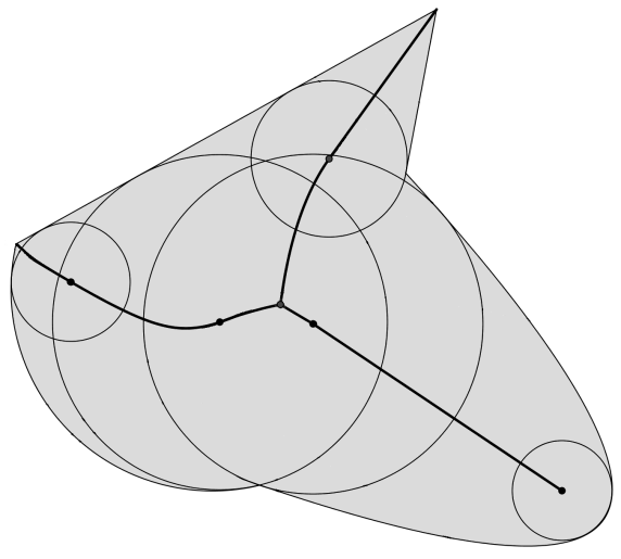
Let be a compact subset of . We will say that a closed ball (possibly of zero radius) is maximal in , if it is not a proper subset of any other ball . The set that consists of the centers of all maximal balls, is called the central set of (see Figure 1 for an example of a central set). We note that typically, the set is infinite.
2.1. Counterexamples with centers in the central set
We start with an observation that can be loosely formulated in the following way: if there exists a counterexample to the Kneser-Poulsen conjecture, then this counterexample can be chosen so that the centers of the balls before the rearrangement lie in the central set of their union.
For a more accurate statement we first introduce some additional notation: for a continuous map that rearranges the centers of the maximal balls in , we denote by the union of these maximal balls after their rearrangement by the map . Now we can state the above observation in a more precise form:
Lemma 2.1.
Let be the union of finitely many closed balls and let be the union of the same balls after a contractive rearrangement. Let be an arbitrary contraction (1-Lipschitz map), such that its restriction to the centers of the balls provides the considered contractive rearrangement. Then the set is compact (hence has a well-defined volume) and . In particular, if , then .
2.2. Structure of the central set
According to Lemma 2.1, in order to prove the Kneser-Poulsen conjecture, it is enough to rule out the counterexamples with (possibly infinitely many) balls, whose centers in the initial configuration lie in the central set of their union. In order to approach this problem, a better understanding of the structure of the central set is required. The following lemma gives a combinatorial and topological description of the central set of the union of finitely many balls.
Definition 2.2.
We will say that a set is an -dimensional ball-polytope, if it can be represented as a union of finitely many closed balls of positive radii, and is a codimension one topological submanifold of .
Lemma 2.3 (Structure lemma).
Let be one of the three spaces , or , where , and let be a ball-polytope. Then the following holds:
(i) the central set has a structure of a finite -dimensional cell complex whose -dimensional cells are -dimensional convex polytopes;
(ii) the set can be represented as the union of finitely many balls with centers at the -dimensional cells of the cell complex ;
(iii) the sets and are homotopy equivalent.
Remark 2.4.
In case if , there is a strong relation between the central set of a ball-polytope and the dual complex (or dual shape ) defined in [14]. More specifically, let be the union of finitely many -dimensional balls with corresponding centers and let be the associated weighted Voronoi cells. We recall that by definition, the convex hull of a subset is a cell of the dual complex , if and only if the dimension of this convex hull is equal to and the intersection of truncated Voronoi cells is nonempty. The dual shape is defined as the union of all cells from . It can be observed from the proof of Lemma 2.3 that for a ball-polytope , the equality holds, if and only if , while in the general case, the central set is a deformation retract of .
2.3. Divide and conquer principle
Let be a closed non-empty subset. We denote by the union of all maximal balls in that are centered at points of .
Now we are ready to formulate the lemma that is crucial for the proposed method.
Lemma 2.5 (Splitting lemma).
Let and be the same as in Lemma 2.3. Let be closed non-empty sets, such that . Then
It is worth mentioning that the inclusion is trivial, while the opposite inclusion is not obvious.
The proof of Lemma 2.5 relies on the properties of a new object that we call a relative central set. We introduce this notion in Section 4.2 for a more general class of compact sets in an arbitrary complete Riemannian manifold.
Lemma 2.5 is called the Splitting lemma, because it provides the groundwork for applying the “divide and conquer” principle and eventually constructing the inductive argument. In order to proceed with the “divide and conquer” principle, we have to introduce some additional notation and formulate a technical lemma.
For a closed set and a contraction that rearranges the centers of the maximal balls in , we let represent the union of the balls that are obtained from all maximal balls in with centers in after these balls are rearranged by the map . Lemma 4.5 proved in Section 4, immediately implies the following statement:
Lemma 2.6.
Let and be the same as in Lemma 2.3, and let be a contraction. Then for any closed non-empty subset , the sets and are compact, and in particular, have a well-defined volume.
We split the configuration of all maximal balls in into two smaller configurations, one with centers in and another – with centers in , so that . Then Lemma 2.5 and Lemma 2.6 imply that the volume of the set can be represented as
| (1) |
An obvious inclusion implies that
| (2) |
In the following proposition we formulate a version of the “divide and conquer” principle, which is sufficient for a proof of Theorem 1.2.
Proposition 2.7.
Let and be the same as in Lemma 2.5, and let be a contraction. If , and , then
We finish this subsection by formulating another technical lemma whose proof will be given in Section 4.
Lemma 2.8.
Let and be the same as in Lemma 2.3. Let be a closed non-empty set and let be the relative boundary of in . If , then .
2.4. Piecewise isometries
In order to construct an inductive argument, it is convenient to work with contractions that can be described combinatorially. We choose piecewise isometries as a class of such contractions.
Definition 2.9.
A map is called a piecewise isometry, if the map is continuous and there exists a locally finite triangulation of , such that for any simplex of that triangulation, the restriction of to is an isometry.
An important ingredient of the proof of Theorem 1.2 is the following extension theorem:
Theorem 2.10.
Proof of Theorem 1.2.
Let be one of the three spaces , or . Assume that there exists a counterexample to the statement of Theorem 1.2. According to Theorem 2.10, the corresponding rearrangement of the centers of the disks can be extended to a piecewise isometry . We fix this piecewise isometry together with the associated triangulation of the space . Without loss of generality we may assume that every interior point of the union of the disks in the initial configuration is also an interior point of some disk. (If an interior point is not in the interior of some disk, then it lies in the intersection of at least two boundary circles. There are finitely many such points and we can always place new small disks that cover them.) We decrease the radii of the disks slightly, if necessary, so that the union of the disks in the initial configuration of the counterexample is a simply connected ball-polytope. Let us denote this ball-polytope by . Since the perturbation of the radii can be arbitrarily small, we may assume that the new configuration of disks still provides a counterexample to the statement of Theorem 1.2. Then Lemma 2.1 implies that
| (3) |
Let be the set of all simply connected ball-polytopes , such that the inequality (3) holds. As we just noticed, the set is non-empty. It follows from Lemma 2.3 that for every , the central set has the structure of a tree with straight edges. Every edge intersects only finitely many simplexes from the triangulation associated to , so it can be split into finitely many edges, such that restricted to each one of them is an isometry.
For , let denote the tree structure on , such that restricted to every edge of is an isometry, and has the smallest possible number of edges. Let denote the number of edges in the graph .
We choose an element with the minimal number . This number is strictly positive, since otherwise is a ball and the inequality (3) does not hold. Now since and is a tree, it has an edge with a vertex of index . Let us denote this edge by and define . Since is a singleton, the sets and are congruent balls, hence their volumes are equal, and since is an isometry on , it follows from Proposition 2.7 that
Moreover, it follows from part (ii) of Lemma 2.3 and from Lemma 2.5 that the set has a form , where are two closed disks centered at the vertexes of the edge . The latter implies that is a simply connected ball-polytope, hence .
Finally, since relative boundary of in is the set that consists of one point, we have , and Lemma 2.8 implies that . Thus , which contradicts the choice of the ball-polytope . ∎
2.5. The general case of the Kneser-Poulsen conjecture
As seen from the proof of Theorem 1.2, in order to apply the same methods to prove the Kneser-Poulsen conjecture in full generality in spaces of arbitrary dimension, one requires a more delicate statement than Proposition 2.7, since we cannot always find a splitting of the central set into two pieces and so that and neither of the sets and is equal to . This is the main obstruction. However, if we can show that there always exists a splitting , such that
then (1) and (2) will imply that
3. Notation
In the remaining part of the paper we will always assume that is a (smooth) complete connected Riemannian manifold, unless otherwise specified. For a point and a positive real number , let represent a closed geodesic ball of radius , centered at . By convention, .
Let be a set and consider two functions, and . We denote by the union of geodesic balls
where runs over all elements of . If is already a subset of and the map is the identity map on , in order to shorten the notation, we will write instead of .
Let be the intrinsic metric on induced by the Riemannian metric tensor. Consider a set . A map is called a contraction, if for every pair of points , the inequality holds.
We also let represent the volume of a set provided that it is defined.
4. Central sets
The goal of this section is to establish some important properties of central sets and prove the lemmas formulated in Section 2. In particular, we introduce the notion of a relative central set and prove that under certain conditions, satisfied by ball-polytopes in , or , the relative central sets are contractible (c.f. Lemma 4.10 for a precise statement). For the sake of possible further generalizations, most of the results about the central sets are proved for subsets of an arbitrary complete connected Riemannian manifold.
We start by giving the definition of the central set of a closed region in a Riemannian manifold .
Definition 4.1.
Let be a closed subset of . A closed geodesic ball is called a maximal ball in , if it is not a proper subset of any other closed geodesic ball contained in and such that .
Definition 4.2.
Let be a closed subset of . A point is a cut point of , if it is a center of a maximal ball in .
Definition 4.3.
The central set of a closed set in is the set of all cut points of . We denote the central set of by . By we denote the map , such that for every , the ball is a maximal ball in .
Lemma 4.4.
Assume that a set and a function are such that the set is compact in . If a map is a contraction, then .
Proof.
Due to compactness of , for every point , the ball is contained in some maximal ball , where is a point from the central set, and . Since the map contracts the distance between centers of the balls, we have , which implies the statement of the lemma. ∎
Let us introduce the following notation: let be a closed set and let be a closed non-empty subset of . For a contraction , we denote by the set . If , then we abbreviate the notation by writing instead of .
Lemma 4.5.
Let be a compact set and let be a closed non-empty set. Then for any contraction , the set is compact.
Proof.
Assume that there exists a point , such that . Then there exists a sequence of points in , such that
| (4) |
From compactness of the set it follows that the sequence has a limit point . Since , the number is strictly positive. Finally, since is a maximal ball in and is a contraction, this implies that for every , such that , we have , which means that there are infinitely many values of , such that
Thus, we arrive at a contradiction with (4). ∎
4.1. Central set of a compact region with smooth boundary
From now on, let be a compact connected subset of , such that is a -smooth codimension one submanifold of . Below we outline some basic facts about the central set. A more rigorous exposition can be found for example in [8]. We note that in the case when is a smooth connected submanifold of , the notion of the central set is strongly related to the notion of the cut locus of . More precisely, is the connected component of the cut locus of that is contained in .
We let denote the unit normal bundle to the submanifold . Every element of the unit normal bundle defines a geodesic on the manifold . Starting from the base point of the vector and moving along this geodesic towards the interior of , we must eventually hit the central set at some point , since otherwise a compact set would contain balls of arbitrarily large radius. We denote by the closed segment of the above geodesic that is contained in and whose endpoints are and . Let be the length of .
Let denote the “distance to the boundary” function. Namely, is the distance from a point to the submanifold . It is well known that the distance must be obtained along some geodesic segment that passes through the point . In particular, this implies that . At the same time it is obvious from the definition of the central set that every point belongs to exactly one geodesic segment . For and we define to be the point on this geodesic segment , such that is distance away from .
We define the function in the following way:
The following statement was essentially proved in Theorem 2 of [22].
Lemma 4.6.
Let the boundary of a compact subset be a -smooth codimension one submanifold of . Then the central set is compact, if and only if the map is a continuous deformation retraction of onto .
Remark 4.7.
It is shown in the same paper [22] that if the boundary is -smooth, then the central set does not have to be compact, while -smoothness of implies compactness of . Even if the boundary is -smooth, the central set can be quite wild. For example, it might be nontriangulable [15]. On the other hand, in [20] it is shown that the function defined by , is Lipschitz, which implies that the canonical interior metric can be introduced on , so that is a locally compact and complete length space.
4.2. Relative central set
The following definition seems to be new, as we were not able to find it in the literature.
Definition 4.8 (Relative central set).
Let be a closed set, and let be the central set of . For a point , we will denote by the central set of relative to which is defined as the set of all points , such that .
We will also need the following definition:
Definition 4.9.
Let be a closed set. A point is called a standard point in , if for every point that can be connected with by two distinct geodesic segments of lengths and respectively, the closed ball is not contained in .
Now we will assume that is a compact connected subset of , such that is a -smooth codimension one submanifold of . The following lemma states that if the central set is compact, then the relative central set of a standard point in is always contractible. This is essentially the key lemma for the proof of Theorem 1.2.
Lemma 4.10.
Let be a compact connected subset, such that is a -smooth codimension one submanifold of , and the central set is compact. Let be a standard point in . Then the set is compact, non-empty and homotopy equivalent to a point.
Proof.
We denote by the set of all points , such that the closed geodesic ball is contained in . It is easy to verify that is a closed subset of and .
Another description of the set can be given in the following way: for every vector with , consider the maximal closed geodesic segment starting at and going in the direction of the vector , such that for every point , the closed geodesic ball is contained in . Since is a standard point in , it follows that , for every pair of distinct unit vectors . Moreover, from this observation and from the construction of geodesic segments it follows that
and is homotopy equivalent to a point.
Finally, we observe that if two points belong to the same geodesic segment defined in Subsection 4.1, and , then . This implies that if , then also . This means that if , then also . From this and from Lemma 4.6 we conclude that the map restricted to the set is a continuous deformation retraction of onto , hence is homotopy equivalent to a point. ∎
Remark 4.11.
If the point is not standard in the set , then the result of Lemma 4.10 might not hold. For example, let be the cylinder and let be the set . Then the central set of as well as the relative central set of the point zero is the unit circle which is not contractible.
Corollary 4.12.
Let be the same as in Lemma 4.10 and assume that every point in is standard. Let be closed non-empty sets, such that . Then
Proof.
The inclusion is obvious. In order to prove that we notice that if a point belongs both to and , then the relative central set has a non-empty intersection both with and with . Since according to Lemma 4.10, the set is connected, the latter implies that has a non-empty intersection with , hence . ∎
4.3. Compact sets with non-smooth boundary
In order to prove Lemma 2.3, Lemma 2.5 and Lemma 2.8 we have to deal with compact sets whose boundary is non-smooth. In this subsection we will assume that is a compact connected set with a non-empty interior, such that is a locally flat codimension one topological submanifold of , and the radius of every maximal ball in is greater than some . Then for any , such that , the function defined by the relation
(where denotes the constant function on ) takes positive values and the set
is compact, connected, and has a non-empty interior.
Proposition 4.13.
For any positive , the boundary is a -smooth codimension one submanifold of .
Proof.
Fix a positive real number , such that
| (5) |
Consider an arbitrary point . Since the point is distance away from , we have . This implies that there exists a unique point and a unique geodesic passing through and , such that the length of its segment between and is minimal and equal to .
Since , there exists a unique maximal ball in , such that . Let be the point on that is distance away from and lies on the other side from . It follows from (5) that , which implies that . From this we conclude that .
Finally, we observe that if is the midpoint of the geodesic segment of between and , then . Thus, is “squeezed” between the two balls and (i.e., intersection of any two of the sets , and is equal to ). Now smoothness of at the point follows. ∎
Let denote the interior of . Since is a locally flat manifold, the collaring theorem of [7] implies that the sets and are homotopy equivalent. It is easy to verify that , for all sufficiently small . Moreover, for all sufficiently small , the functions and (which are defined because of Proposition 4.13) coincide on their common domain of definition , hence the functions converge point-wise to a function
as . It follows from Remark 4.7, that the map is not necessarily continuous. On the other hand, the fact that together with Lemma 4.6 implies the following statement:
Lemma 4.14.
Let be a compact connected set with a non-empty interior, such that is a locally flat codimension one topological submanifold of , and every maximal ball in has positive radius. Then the central set is compact, if and only if the map is a continuous deformation retraction of onto .
The following lemma is an analog of Corollary 4.12.
Lemma 4.15.
Let be a compact connected set with a non-empty interior, such that the following holds:
-
•
is a locally flat codimension one topological submanifold of ;
-
•
every maximal ball in has positive radius;
-
•
the central set is compact;
-
•
every point in is standard.
Let be closed non-empty sets, such that . Then
Proof.
The inclusion is obvious. Let us prove the opposite inclusion. First, assume that is an interior point of . Then there exists a positive , such that , hence by Corollary 4.12, we have , which implies that .
Finally, since all maximal balls in have positive radius, every point is a limit point of the interior of , hence by the previous case we have . Since according to Lemma 4.5, the set is closed, this implies that . ∎
If is a closed set, Lemma 4.5 says that the set is compact, hence we can consider its central set which we will denote by . It is easy to see that , while the opposite inclusion does not necessarily hold.
Lemma 4.16.
Let be the same as in Lemma 4.15, and let be closed non-empty sets, such that is the relative boundary of in . If , then .
Proof.
If a maximal ball in is contained in , then it is also a maximal ball in , since . Thus . This means that in order to prove the lemma, it is enough to show the opposite inclusion.
Define the set as the closure . Then . We proceed with a proof by contradiction. Assume that there exists a ball that is a maximal ball in and whose center is not in . Then there exists a ball centered outside of , such that is maximal in and . Since , this implies that the center of the ball belongs to , and . Hence, we have , and then, according to Lemma 4.15, we have . Since the ball is maximal in and , the ball is also maximal in , hence, its center belongs to . Finally, since , we obtain a contradiction. Thus we have . ∎
Finally, we pass to the proof of Lemma 2.3.
Proof of Lemma 2.3.
Let be one of the three spaces , or , and let be -dimensional closed balls of positive radius, such that
is an -dimensional ball-polytope. By definition of a ball-polytope, the boundary is a topological manifold of dimension .
Let be a family that consists of all connected components of all intersections of the form
where runs over all subsets of the set . Clearly, is a finite family, and
A set from will be called a cell of . Every cell lies in the intersection of finitely many -dimensional spheres, so if is not a single point, then there exists a minimal positive integer , for which there is a unique -dimensional sphere in that contains the cell . We denote this sphere by . For every we let represent the set of all , for which the sphere is -dimensional, and we denote by the set of all that are singletons. Thus, is a disjoint union
We will say that a cell has dimension , if .
Definition 4.17.
For a cell , we will say that a point is an interior point of , if it does not belong to any cell of dimension strictly smaller than .
In particular, every -dimensional cell consists of one point that is an interior point of .
For future reference let us formulate the following basic geometric facts:
Proposition 4.18.
Every point is an interior point of some cell .
Proposition 4.19.
Let be a cell of positive dimension. Then is an interior point of , if and only if belongs only to those spheres which contain the sphere .
Now we prove the following statement:
Proposition 4.20.
If the boundary sphere of a maximal ball in contains an interior point of a positive dimensional cell , then this sphere contains the whole cell .
Proof.
Let be an interior point of that also belongs to the boundary of an -dimensional ball . Assume that is a maximal ball in . We will show that . We split the proof into two cases:
Case 1: We weaken the assumption on the set by requiring to be a submanifold only locally at point . At the same time we assume that , for all . Then in particular we have
| (6) |
Let be another point, where touches , and let be the set of all indexes , such that . Consider the sphere
According to (6), we have an inclusion , hence, is a common point of and . Since the spheres and must also be tangent at the point , and , this implies that , and in particular, .
Case 2: Now we consider the general case. Let be the set of all integers , such that . Consider the set . Since is a ball-polytope, it follows from Proposition 4.19 that is a local manifold around the point , and there exists an -dimensional ball that is maximal in , and whose boundary sphere is tangent to at . Now Case 1 implies that , and since is contained in and cannot have common points with the interior of , we conclude that and . ∎
Let be a finite set, such that for every cell , the set is non-empty, and for every positive-dimensional cell , the affine span of has dimension . We notice that the existence of such a set follows from the fact that the family is finite.
Let us formulate the statement that is a straightforward consequence of the assumption on .
Proposition 4.21.
For every cell , an -dimensional sphere contains the set , if and only if this sphere contains the whole cell .
The following proposition immediately implies part (i) of Lemma 2.3.
Proposition 4.22.
The central set is a subcomplex of the -skeleton of the Voronoi cell decomposition of the set .
Proof.
First, let us prove that the central set is contained in the -skeleton of the Voronoi cell decomposition of the set . In order to do this, it is enough to show that the boundary sphere of every maximal ball in contains at least two distinct points from . This can be shown in the following way: the boundary sphere of every maximal ball in contains at least two distinct points from . If both of these points form -dimensional cells from , then by the assumption on , these two points belong to . If at least one of these two points does not belong to a -dimensional cell from , then, by Proposition 4.18, it is an interior point of some positive dimensional cell . In this case, Proposition 4.20 implies that the whole cell is contained in the boundary sphere of the maximal ball. In particular, according to the assumption on , this means that at least two distinct points from belong to this boundary sphere.
Now we claim that if an interior point of an -dimensional Voronoi cell belongs to , then the whole cell is contained in as well. Indeed, every -dimensional Voronoi cell corresponds to some subset with the property that for every point there exists an -dimensional sphere that is centered at and contains the set , and if is an interior point of , then the corresponding sphere does not contain any other points from . Then Proposition 4.21 implies that there exists a collection of cells , such that for every interior point , the sphere contains precisely the cells from and no other cells from .
Assume that there exists an interior point of the cell , such that , and a point , such that . This is equivalent to the statement that is the boundary sphere of a maximal ball in , but is not. In other words, there are no points of in the interior of the sphere , and there are such points in the interior of the sphere . We connect the points and by a geodesic segment . Since is convex, all points of , except possibly the point , lie in the interior of . Since the sphere depends continuously (in Hausdorff topology) on the point , there exists an intermediate point , , with the property that for all lying between and , there are no points of in the interior of the sphere , and for all sufficiently close to but lying between and , such points of exist. Then continuous dependence of on implies that the sphere is the boundary sphere of a maximal ball in , and must contain a point that does not belong to any of the cells from . According to Proposition 4.18, there exists a cell , such that and is either an interior point of , or . In both cases either Proposition 4.20 or the fact that is a singleton, imply that the cell is a subset of . The latter contradicts to the fact that is an interior point of . ∎
In order to prove part (ii) of Lemma 2.3, we notice that the -dimensional cells of the family cover the whole boundary of the ball-polytope . This implies that the maximal balls centered at all -dimensional cells of , cover the whole set .
References
- [1] A. V. Akopyan and A. S. Tarasov. A constructive proof of Kirszbraun’s theorem. Mat. Zametki, 84(5):781–784, 2008.
- [2] M. Bern and A. Sahai. Pushing disks together—the continuous-motion case. Discrete Comput. Geom., 20(4):499–514, 1998.
- [3] Károly Bezdek and Robert Connelly. Pushing disks apart—the Kneser-Poulsen conjecture in the plane. J. Reine Angew. Math., 553:221–236, 2002.
- [4] Károly Bezdek and Robert Connelly. The Kneser-Poulsen conjecture for spherical polytopes. Discrete Comput. Geom., 32(1):101–106, 2004.
- [5] B. Bollobás. Area of the union of disks. Elem. Math., 23:60–61, 1968.
- [6] Ulrich Brehm. Extensions of distance reducing mappings to piecewise congruent mappings on . J. Geom., 16(2):187–193, 1981.
- [7] Morton Brown. Locally flat imbeddings of topological manifolds. Ann. of Math. (2), 75:331–341, 1962.
- [8] Isaac Chavel. Riemannian geometry, volume 98 of Cambridge Studies in Advanced Mathematics. Cambridge University Press, Cambridge, second edition, 2006. A modern introduction.
- [9] B. Csikós. On the Hadwiger-Kneser-Poulsen conjecture. In Intuitive geometry (Budapest, 1995), volume 6 of Bolyai Soc. Math. Stud., pages 291–299. János Bolyai Math. Soc., Budapest, 1997.
- [10] B. Csikós. On the volume of the union of balls. Discrete Comput. Geom., 20(4):449–461, 1998.
- [11] Balázs Csikós. On the volume of flowers in space forms. Geom. Dedicata, 86(1-3):59–79, 2001.
- [12] Balázs Csikós. A Schläfli-type formula for polytopes with curved faces and its application to the Kneser-Poulsen conjecture. Monatsh. Math., 147(4):273–292, 2006.
- [13] Balázs Csikós and Dávid Kunszenti-Kovács. On the extendability of the Kneser-Poulsen conjecture to Riemannian manifolds. Adv. Geom., 10(2):197–204, 2010.
- [14] H. Edelsbrunner. The union of balls and its dual shape. Discrete Comput. Geom., 13(3-4):415–440, 1995.
- [15] Herman Gluck and David Singer. Scattering of geodesic fields. I. Ann. of Math. (2), 108(2):347–372, 1978.
- [16] Igors Gorbovickis. Strict Kneser-Poulsen conjecture for large radii. Geom. Dedicata, 162:95–107, 2013.
- [17] Igors Gorbovickis. Kneser-Poulsen conjecture for a small number of intersections. Contrib. Discrete Math., 9(1):1–10, 2014.
- [18] Y. Gordon and M. Meyer. On the volume of unions and intersections of balls in Euclidean space. In Geometric aspects of functional analysis (Israel, 1992–1994), volume 77 of Oper. Theory Adv. Appl., pages 91–101. Birkhäuser, Basel, 1995.
- [19] M. Gromov. Monotonicity of the volume of intersection of balls. In Geometrical aspects of functional analysis (1985/86), volume 1267 of Lecture Notes in Math., pages 1–4. Springer, Berlin, 1987.
- [20] Jin-ichi Itoh and Minoru Tanaka. The Lipschitz continuity of the distance function to the cut locus. Trans. Amer. Math. Soc., 353(1):21–40, 2001.
- [21] Martin Kneser. Einige Bemerkungen über das Minkowskische Flächenmass. Arch. Math. (Basel), 6:382–390, 1955.
- [22] David Milman and Zeev Waksman. On topological properties of the central set of a bounded domain in . J. Geom., 15(1):1–7, 1981.
- [23] Ebbe Thue Poulsen. Problem 10. Math. Scand., 2:346, 1954.
- [24] F. A. Valentine. A Lipschitz condition preserving extension for a vector function. Amer. J. Math., 67:83–93, 1945.