Abstract

We present a new method for obtaining the statistical weight of the Gentile Statistics. In a recent paper, Perez and Tun presented an approximate combinatoric and an exact recursive formula for the statistical weight of Gentile Statistics, beginning from bosonic and fermionic cases, respectively [1]. In this paper, we obtain two exact, one combinatoric and one recursive, formulae for the statistical weight of Gentile Statistics, by an another approach. The combinatoric formula is valid only for special cases, whereas recursive formula is valid for all possible cases. Moreover, for a given q-maximum number of particles that can occupy a level for Gentile statistics-the recursive formula we have derived gives the result much faster than the recursive formula presented in [1], when one uses a computer program. Moreover we obtained the statistical weight for the distribution proposed by Dai and Xie in Ref. [2].
Keywords: Fractional statistics, Gentile distribution, Statistical Weight

———————————————————————

1 Introduction

An interesting property of low dimensional systems is that the particles in these systems may obey different statistics other than Bose-Einstein and Fermi-Dirac statistics [3] . Following the realization that there can be quasi particles, whose many body wave function may have a general phase $e^{i\theta}$ [4, 5, 6] -other than $1$ or $(-1)$-, Haldene proposed a fractional statistics in arbitrary dimensions [7]. Then, Wu derived statistical weight for the Haldene fractional statistics [8]

$$W_{i}=\frac{[g_{i}+(n_{i}-1)(1-\alpha)]!}{n_{i}![g_{i}-\alpha n_{i}-(1-\alpha)]!}.$$ (1)

Here, $n_{i}$ gives the identical number of particles occupying a state $i$ and $g_{i}$ is the number of states. The parameter $\alpha$ in Eq.(1) yields an interpolation between Bose-Einstein and Fermi-Dirac statistics. So, the statistical weight Wi in $(1)$ reduces to Bose-Einstein and Fermi-Dirac statistics, for $\alpha=0$ and $\alpha=1$, respectively. On the other hand, Polychranakos suggested another form for the statistical weight of the Haldene fractional statistics [9].

The possibility of intermediate statistics led to the new studies on Gentile Statistics, which was proposed much before than the other generalizations of the Bose-Einstein and Fermi-Dirac statistics [10]. For example, Dut et. al have shown that the expressions for distribution and other thermodynamic quantities derived using Gentile statistics are also valid for a q-fermion provided q is a complex number and takes values on a unit circle [11]. Then, Chaturvedi and Srinivasan compared different interpolations between Fermi and Bose Statistics including Gentile statistics [12]. Bysto derived a thermodynamic Bethe ansatz equation for relativistic particles obeying generalized extensive statistics [13]. Moreover, Dai and Xie showed that Gentile statistics does not reduce to Bose-Einstein statistics generally but only if fugacity $z=e^{\beta\mu}<1$ [14]. In addition to that, they show that one can obtain Bose-Einstein distribution $f_{BE}$, from Gentile distribution $f_{G}$, in thermodynamic limit when one takes two limits, maximum occupation number $q\rightarrow\infty$, and the total number of particles $(N\rightarrow\infty)$ in a given order $(f_{BE}\equiv\lim_{<N>\rightarrow\infty}{\lim_{n\rightarrow\infty}f_{G}})$ [15]. Furthermore, Donald and Zly derived thermodynamic properties for a harmonically confined gas obeying Gentile statistics in d-dimensions and compared these results with a similar system obeying Haldene-Wu statistics [16].

There are also rather mathematical studies about Gentile statistics. For example, the relationship between Gentile statistics and restricted partitions is investigated by Srivatson et. al. [17]. Moreover, Niven studied the combinatorial entropies and statistics [18], and Mirza and Mohommadzeh investigated thermodynamics geometry of fractional statistics [19].

It is also possible to obtain intermediate statistics from operator relations. For example Melijenac et. al. studied exclusion statistics in the second quantized approach which includes Gentile statistics as a special case [20]. In addition to that, Dai and Xie obtained an operator realization for the angular momentum algebra which naturally leads to Gentile distribution [21]. Whet significant in this derivation is that one does not need to restrict the number of the particles by fiat as it is done in the Holstein-Primakoff representation [22] because it arises naturally in this representation [21]. Then they applied this distribution to the excitations of the spin magnetic waves for the one dimensional Heisenberg chain and showed that the distribution they have obtained explains the excitation spectrum better than the Hollstein-Primakoff method [21]. Moreover, the same authors derived Gentile statistics from operator relations [23]. In this study, the authors used an algebra similar to that of the one dimensional harmonic oscillator algebra but in this algebra creation and annihilation operators are not hermitian conjugate of each other. Using this more generalized algebra, they showed that in the algebras where a number operator $\hat{N}$ can be defined a quadratic function of creation and annihilation operators one gets the Gentile distribution corresponding to this algebra [23].

Recently, several studies showed that, Gentile statistics can also be used to describe realistic physical systems. Indeed, Gentile statistics is appropriate for investigating two dimensional electron gases in two dimension when the electrons are so dilute that the Coulomb interactions between them is negligible. In this case, the behavior of the electrons is described by a Hamiltonian similar to the harmonic oscillator hamiltonian but having one more degree of freedom. Therefore, more than two electrons (including spin degeneracy) may occupy each single particle states but the maximum number of the electrons in a state is limited by the magnetic field leading to the de Haas-van Alphen effect [24]. The statistical distribution of these electrons is the Gentile distribution. Moreover, Auccaise et.al. presented a description of nuclear magnetic resonance of quadrupolar system [25]. In this work, using Holstein-Primakoff representation [22] the authors proposed that NMR quadrupolar system have BEC like behavior and they experimentally verified their results for two different quadrapol nuclei (${}^{23}Na$) and (${}^{133}Cs$) in lyotropic cyrstals which have nuclear spins $I=3/2$ and $I=7/2$, respectively. These system are interesting because their statical properties may be obtained using the Gentile statistics[25]. Moreover, Shen and Yin showed that cyclich hydrocarbon polyenes $C_{N}H_{N}$, called N-annules, are physical realizations of Gentile systems [26].

In this paper, we present a new inductive method to obtain the statistical weight of the Gentile statistics. The statistical weight for Gentile statistics is first derived by Perez and Tun [1]. We will derive two formulae one combinatoric and one recursive like in [1]. Both formulae are exact but the combinatoric one is valid only for special cases. Since, the statistical weight for Gentile statistics is derived earlier in [1], we owe to an explanation why we have done this study. We obtain an exact combinatoric formula for all q values, maximum number of particles which can occupy a state, which however is only valid for $(G-1)q\leq N\leq Gq$ , where $N$ is total number of the particle and $G$ is the number of different states, respectively. The combinatoric formula obtained in [1] is valid only for $q\geq N/2$. The recursive formulae are useful only when one uses computers, and the recursive formula we obtained produces the statistical weight much faster, compared to the recursive formula obtained in [1], when $q$ has a determined value like in $N$ annules [26]. Moreover, the inductive method constructed in this work can be applied to find the statistic weight constructed in [2] by Xie and Dai which is more general than Gentile statistics. We will denote this statistics as Dai-Xie distribution.

2 Method

In this section, we will present a new inductive method for obtaining the statistical weight of Gentile statistics. This method can also be used to obtain the statistical weight for Bose-Einstein statistics. For the sake of simplicity, we first apply the method for obtaining the statistical weight of Bose-Einstein statistics.

The statistical weight for bosons give the number of different ways of distributing N bosons to G levels, $R(N,G)$. Since our method is inductive, we first find how many different ways to distribute N bosons to two levels. (Obviously, there is only one way to distribute N bosons to one level.)

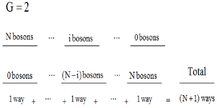
Figure 1: Statistical weight of N bosons for two levels $R(N,2)$

In order to find the number of ways to distribute N bosons to two levels $R(2,N)$, we count all different cases (see Figure 1). There can be $0$ bosons in level $2$ and all bosons can be level $1$. Or, there can be $1$ boson in level $2$ and $N-1$ bosons in level $1$, $2$ bosons in level $2$ and $N-2$ bosons in level $1$ and so on. Counting the different cases, we find that there are $(N+1)$ ways to distribute $N$ bosons two levels. Now, we will find $R(3,N)$ using $R(2,N)$. We again use the same logic. We assume first there are $0$ bosons in level 1. Thus there are $N$ bosons in level $2$ and $3$. Since we know $R(2,N)=N+1$, we conclude if there are $0$ bosons in level 2, then three are $(N+1)$ ways to distribute $N$ bosons to there levels (see Figure 2). If, there is only one boson in level two, there are $N-1$ bosons in level $2$ and $3$. Therefore, in this case, there are $R(2,N-1)=N$ different ways to distribute $N$ bosons to three levels. By using the same logic one can conclude, if there are two bosons in level $1$ there are $N-1$, if there are three bosons in level $1$ there are $N-2$ ways to distribute $N$ bosons to three levels and so on. Generally, if there are $i$ bosons in level $1$, there are $(N+1-i)$ ways to distribute $N$ bosons to three levels. Since there can be at least $0$ bosons and at most $N$ bosons in level $1$, the total number of ways to distribute $N$ bosons to three levels is

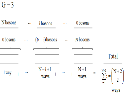
Figure 2: Statistical weight of N bosons for three levels $R(N,3)$

$$R(3,N)=\sum_{i=1}^{N}(N+1-i)=\sum_{j=1}^{N+1}j=\frac{(N+1)(N+2)}{2}=\left(\begin{array}[]{c}N+2\\ 2\end{array}\right).$$ (2)

Similarly, it is easy to find $R(4,N)=\left(\begin{array}[]{c}N+3\\ 3\end{array}\right)$. Using results for $R(3,N)$ and $R(4,N)$ we infer a general formula to distribute N bosons to G Levels:

$$R(G,N)=\left(\begin{array}[]{c}N+G-1\\ G-1\end{array}\right).$$ (3)

Now, we have to show that $R(G+1,N)=\left(\begin{array}[]{c}N+G\\ G\end{array}\right)$ assuming Eq. (3) is valid to complete the induction. To do this, we use the method we have used to find $R(2,N)$ and $R(3,N)$. We first assume that there $0$ bosons in level $1$. Thus, there are N bosons in the remaining G levels and $R(G,N)=\left(\begin{array}[]{c}N+G-1\\ G-1\end{array}\right)$ different ways to distribute $N$ bosons to these levels. If there are $1$ boson in the first level, then there are $R(G,N-1)=\left(\begin{array}[]{c}N-1+G-1\\ G-1\end{array}\right)$ ways to distribute remaining $N-1$ bosons to the G groups. Continuing this process and summing the number of all different ways for the different numbers of bosons in level $1$ we get

$$R(G+1,N)=\sum_{i=0}^{N}\left(\begin{array}[]{c}N+G-1-i\\ G-1\end{array}\right),$$

$$\sum_{k=G-1}^{N+G-1}\left(\begin{array}[]{c}k\\ G-1\end{array}\right)=\left(\begin{array}[]{c}N+G\\ G\end{array}\right).$$ (4)

In order to get third term from the second one in Eq. (4) we have changed the dummy index $i$ to $k=N+G-1-i$. Moreover we have used the equality $\sum_{j=m}^{n}\left(\begin{array}[]{c}j\\ m\end{array}\right)=\left(\begin{array}[]{c}n+1\\ m+1\end{array}\right)$ for $n\geq m$. Since Eq. (4) is the same as the Eq. (3) for $G$ replaced by $(G+1)$, we conclude that our assumption namely Eq. (3) is valid.

The inductive method we have introduced in the previous paragraphs can also be used to find the statistical weight for systems obeying Gentile distribution (Gentile particles). For Gentile particles there is an upper limit for the number of particles that can occupy a level and we denote this limit by q. By using the inductive method for Gentile particles one has to take this limit into account.

We will now find the the statistical weight for Gentile particles. Following the notation introduced in [1], we will denote the statistical weight for Gentile particles by $R_{q}(G,N)$ which shows the number of different ways to distribute $N$ particles into $G$ levels for a given q. The total number of Gentile particles for given $G$ and $q$ has an upper limit $N_{max}=Gq$.

We first investigate the case $N\leq q$. In this case, $R_{q}(G,N)$ is the same as the boson distribution for all $G$. Since the limit $q$ is greater than the total number of particles it does not effect the occupancy of a level . Therefore we can write

$$R_{q}(G,N)=\left(\begin{array}[]{c}N+G-1\\ G-1\end{array}\right)\;\;\;\;\;\;\;\;\;\;N\leq q.$$ (5)

In order to find the statistical weight for all cases, we again start with two levels, i.e., we will first calculate $R_{q}(2,N)$. We will separate the cases $q<N\leq 2q$ and $N\leq q$. Since for $q\geq N$ the statistical weight for Gentile particles is the same as the statistical weight for bosons, we get

$$R_{q}(2,N)=R(2,N)=(N+1)\qquad N\geq q$$ (6)

If $q<N\leq 2q$, we count the number of different ways, separating level $1$. One can put minimum $N-q$ (otherwise there would be more than $q$ particles in level $2$, which is not allowed for Gentile particles), maximum q particles to level 1. Since there is only one level left, there is only one way to distribute the remaining particles to the remaining level. Therefore, there are $2q+1-N$ number of ways to distribute $N$ particles to two levels if $q<N\leq 2q$. Hence, we can write

$$R_{q}(2,N)=\begin{cases}2q+1-N\;\;\;\;\;\;q\leq N\leq 2q\\ N+1\;\;\;\;\;\;N\leq q\end{cases}$$ (7)

The two equalities in Eq. (7) give the same number for $N=q$. So one can use any of them for this case.

We will now try to find $R_{q}(3,N)$. Since the case $N\leq q$, is boson distribution we will try to find $R_{q}(3,N)$ for $N>q$. We separate cases $2q\leq N\leq 3q$ and $N<2q$. Because the formula for $R_{q}(2,N)$ differs for cases $q\leq N$ and $N<q$. If there are more than $2q$ Gentile particles to distribute to three levels, the total number of particles in the levels 1 and 2 has to be more than $q$, because we can put at most $q$ particles to level $1$. Therefore, one can see from Eq. (7) that the expression for the statistical weight differ for $2q\leq N\leq 3q$ and for $N<2q$.

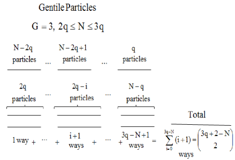
Figure 3: Statistical weight of N Gentile particles for three levels $R_{q}(N,3)$ when $2q\leq N\leq 3q$

We first begin with the case $2q\leq N\leq 3q$. We will use the first equality in Eq. (7) for $R_{q}(2,N)$, because the total number of particles in the levels 2 and 3 is more than $q$ for this case, as mentioned above. One can put at least $(N-2q)$ and at most $q$ particles to level $1$ . If there are $(N-2q)$ particles in level 1, one finds from Eq. (7) that there are only $2q+1-2q=1$ way to distribute remaining $2q$ particles into two levels. If there are $i$ particles in level 1, there are $[2q+1-(N-i)]$ ways of distributing remaining $(N-i)$ particles to the remaining two levels (see Figure 3). Hence for $2q\leq N\leq 3q$ one obtains

$$R_{q}(3,N)=\sum_{i=N-2q}^{q}2q+1-(N-i)=\left(\begin{array}[]{c}3q+2-N\\ 2\end{array}\right)\quad 2q\leq N\leq 3q.$$ (8)

For $q<N<2q$ one can use the same logic but one must be careful. Because now it is possible to put $0$ to $q$ particles to level 1 and the formula will change depending whether there are less than $N-q$ particles in level $1$ or more than $N-q$ particles in level $1$. Because if there less than $(N-q)$ particles in level $1$ there are more than $q$ particles in the remaining two levels and one uses the first expression in Eq. (7) for $R_{q}(2,N)$. If there are more than $N-q$ particles in level $1$, there are less than $q$ particles in the remaining two levels and one uses the second expression in (7) for $R_{q}(2,N)$. So, $R_{q}(3,N)$ for $q<N<2q$ is

$$R_{q}(3,N)=\sum_{i=0}^{N-q}[2q+1-(N-1)]+\sum_{i=N-q}^{q}(N-i+1)$$ (9)

$$\frac{(q+1)(2N+2-3q)+2(2q-N)(N+1)}{2}.$$

As one may notice this formula can not be written as a combinatoric formula. Therefore, we continue cases where $N$ is between $(G-1)q$ and $Gq$, first. If the number of levels is $4$ and if there are $(3q\leq)N(\leq 4q)$ particles to distribute to these $4$ levels there can be at least $N-3q$, at most $q$ particles in level 1. Using the Eq. (8) one can easily find the number of ways for distributing the remaining particles to the remaining three groups and summing these results one gets

$$R_{q}(4,N)=\sum_{i=N-3q}^{q}\left(\begin{array}[]{c}3q+1-(N-i)\\ 2\end{array}\right)=\left(\begin{array}[]{c}4q+3-N\\ 3\end{array}\right)\;\;\;\;3q\leq N\leq 4q.$$ (14)

From the formulae (7),(8) and (14) we propose that for $(G-1)q\leq N\leq Gq$,

$$R_{q}(G,N)=\left(\begin{array}[]{c}Gq+G-1-N\\ G-1\end{array}\right).$$ (15)

Assuming Eq. (15) is true, it is easy to prove $R_{q}(G+1,N)=\left(\begin{array}[]{c}(G+1)q+G-N\\ G\end{array}\right)$. This is done by the logic we have used for all cases until now: We separate level $1$ from other $G$ levels, then find for all number of allowed number of particles $(i)$ in level $1$ the number of different ways to distribute remaining $(N-i)$ particles to the remaining $G$ levels $R_{q}(G,N-i)$ using Eq. (15) and finally sum $R_{q}(G,N-i)$ for all allowed $i$. Since we are, for now, interested in the case $Gq\leq N\leq(G+1)q$, there can be at least $N-Gq$, at most $q$ particles in level 1. Thus

$$R_{q}(G+1,N)=\sum_{i=N-Gq}^{q}\left(\begin{array}[]{c}Gq+G-1-(N-i)\\ G-1\end{array}\right)=\left(\begin{array}[]{c}(G+1)q+G-N\\ G\end{array}\right)$$ (20)

$$\textrm{where~{}}Gq\leq N\leq(G+1)q$$ (21)

This formula is the same as the Eq. (15) for $G$ replaced by $G+1$. Thus, we have shown by induction that the Eq. (15) gives the statistical weight for Gentile particles when $(G-1)q\leq N\leq Gq$.

One can see from the Eq.(9) if $N<(G-1)q$ for given $G$ and $q$, it is not possible to find a combinatoric formula for the statistical weight of Gentile particles. However, the inductive method can still be used. In this case, one can derive an recursive formula using the inductive method. In order to find $R_{q}(G,N)$ for $N<(G-1)q$, we again separate level $1$ from the remaining $G-1$ levels. Since $N$ is less than $(G-1)q$, at least $0$ bosons, at most $q$ bosons may occupy level $1$. If there are $i$ particles in level $1$, there are $N-i$ particles the remaining $G-1$ levels and there are $R_{q}(G-1,N-i)$ ways to distribute these particles to the remaining $G-1$ levels. Therefore we can write

$$R_{q}(G,N)=\sum_{i=0}^{q}R_{q}(G-1,N-i).$$ (22)

We know $R_{q}(G,N)$ for small $N$ values: $R_{q}(G,N)$ is the same as the statistical weight for bosons if $N\leq q$, that is

$$R_{q}(G,N)=\left(\begin{array}[]{c}N+G-1\\ N\end{array}\right)\;\;\;\;\;\;\;\;N\leq q.$$ (23)

So, for a given $q$, beginning from the statistical weights of small $G$ and $N$ values and utilizing Eq. (23) when possible, it is easy to calculate $R_{q}(G,N)$ recursively, by means of a computer program. In the next section, we will first compare this recursive formula with the recursive formula obtained by Perez and Tun (the Eq. (4) in [1]).

The inductive method developed here is also applicable to the statistics constructed in [2] by Xie and Dai which is more general than Gentile statistics. In this statistics the value of the variable q that is the maximum number of particles that can occupy a state is not constant but may change in other words also the value of the q is state dependent. Therefore we label the maximum number of particles for different state by $q_{i}$ where $i=1,2,..G$. The order of labelling is not important in the calculation of the statistical weight. Therefore we arrange the states such that the inequalities

$$q_{1}\leq q_{2}\leq\ldots\leq q_{G}$$ (24)

are satisfied. In this case the maximum number of particles that can be distributed to the $G$ levels are

$$N_{max}=\sum_{i=1}^{G}q_{i}$$ (25)

We will first show that the combinatoric formula given in Eq. (15) can be extended for this case if the total number of particles $N$ satisfies the inequality $N_{max}-q_{1}\leq N\leq N_{max}$.

We will begin with two states as in the case of Gentile statistics. We assume that there are two states. These states can be occupied by at most $q_{1}$ and $q_{2}$ particles and we order them such that $q_{1}\leq q_{2}$. If $N\leq q_{1}$ the distribution is similar to the bosonic case and thus $R_{\{q\}}(G,N)=N+1$ . If $q_{1}\leq N\leq q_{2}$ then there can be at least $N-q_{1}$ and at most $N$ particles in the second state. Therefore $R_{\{q\}}(2,N))=q_{1}+1$. If $q_{2}\leq N\leq N_{max}=q_{1}+q_{2}$ then there can be at least $N-q_{1}$ and at most $q_{2}$ particles in the state two and thus $R_{\{q\}}(2,N)=N_{max}-N+1$. We can summarize the results obtained for the statistical weight $R_{\{q\}}(2,N)$ as

$$R_{\{q\}}(2,N)=\begin{cases}N_{max}+1-N=\left(\begin{array}[]{c}N_{max}+1-N\\ 1\end{array}\right)&q_{2}\leq N\leq N_{max}\;\;(a)\\ q_{1}+1&q_{1}\leq N\leq q_{2}\;\;\;\;\quad(b)\\ N+1&N\leq q_{1}\;\;\;\;\,\qquad\quad(c)\end{cases}$$ (26)

Using the results obtained for two states, we will find a combinatoric formula for three states if $N_{max}-q_{1}\leq N\leq N_{max}=q_{1}+q_{2}+q_{3}$. (For the other cases it is not possible to find a combinatoric formula and we will derive a recursive formula as in the Gentile statistics later.) Given condition $N_{max}-q_{1}\leq N$ and the fact that at most $q_{3}$ particle can occupy the state 3, there can be at least $N-q_{3}$ particles in the state 3. Because we assume that the lower limit for the total number of particles is $N_{max}-q_{1}=q_{2}+q_{3}$, $N-q_{3}$ is larger or equal to $q_{2}$ and we can use the condition (a) in the Eq. (26) for calculating the total number of different ways of distributing the remaining particles to the remaining two states. If there are $i$ particles in the state 3 there will be $N-i$ particles in the remaining two states and hence we get after some elementary calculations

$$R_{\{q\}}(3,N) = \sum_{i=N-(N_{max}-q_{3})}^{q_{3}}\left[N_{max}-q_{3}-(N-i)+1\right]$$ (29)

$$= \left(\begin{array}[]{c}N_{max}+2-N\\ 2\end{array}\right)\;\;\;\textrm{for~{}}N_{max}-q_{1}\leq N\leq N_{max}.$$

As in the case of Gentile statistics using the part (a) of Eq. (26) and Eq. (29) we propose that the formula for a general number of states $G$ is

$$R_{\{q\}}(G,N)=\left(\begin{array}[]{c}N_{max}+G-1-N\\ G-1\end{array}\right)\;\;\;\textrm{for~{}}N_{max}-q_{1}\leq N\leq N_{max}.$$ (30)

where $N_{max}$ is given by Eq. (25). Then assuming the Eq. (30) is valid we will get the same formula $G+1$ states. In this case $N_{max}=\sum_{i}^{G+1}q_{i}$. We assume again that the total number of particles satisfy $N_{max}-q_{1}\leq N\leq N_{max}$. There can be at most $q_{G+1}$ particles in the state $G+1$. Since $N\geq N_{max}-q_{1}=q_{2}+\ldots+q_{G+1}$ the number of particles in the remaining states always satisfy the necessary inequality given for Eq. (30). Since there can be at least $N-N_{maxG}$ and at most $q_{G+1}$ particles in the state $G+1$ and we assume Eq. (30) is valid we get

$$R_{\{q\}}(G+1,N) = \sum_{i=N-N_{maxG}}^{q_{G+1}}\left(\begin{array}[]{c}N_{maxG}+G-1-(N-i)\\ G-1\end{array}\right)$$ (33)

for $$N_{max}-q_{1}\leq N\leq N_{max}.$$ (34)

where $N_{maxG}=\sum_{i=1}^{G}q_{i}$. Changing the dummy index as $k=i-(N-N_{maxG})$ and using $\sum_{j=m}^{n}\left(\begin{array}[]{c}j\\ m\end{array}\right)=\left(\begin{array}[]{c}n+1\\ m+1\end{array}\right)$ for $n\geq m$ we get

$$R_{\{q\}}(G+1,N) = \sum_{k=0}^{N_{max}-N}\left(\begin{array}[]{c}k+G-1\\ G-1\end{array}\right)=\sum_{k=G+1}^{N_{max}-N+G-1}\left(\begin{array}[]{c}k\\ G-1\end{array}\right)$$ (39)

$$= \left(\begin{array}[]{c}N_{max}-N+G\\ G\end{array}\right)\;\,\textrm{for~{}}N_{max}-q_{1}\leq N\leq N_{max}$$ (42)

Since this equation is the same equation with Eq. (30) for $G$ is replaced by $G+1$, we conclude that the statistical weight for Xie-Dai distribution is given by Eq. (30) if $N_{max}-q_{1}\leq N\ leqN_{max}$. Note that if all $q_{i}$s are equal to each other Then $N_{max}=Gq$ and Eq. (30) reduces Eq. (15) as it must be.

Now we will derive a recursive formula for Xie-Dai statistics because like in the case of the Gentile statistics it is not possible to derive a combinatoric formula if $q_{1}<N<N_{max}-q_{1}$. The recursive formula we will derive is valid for all possible cases. We will again use induction and separate the state G from the other $G-1$ states. If $N>N_{max}-q_{1}$ there can be at least $N-N_{max}$ particles and if $N\leq N_{max}-q_{1}$ there can be at least 0 particles in the state $G$. If $N>q_{G}$ then there can be at most $q_{G}$ but if $q_{G}<N$ there can be at most $N$ particles in the state $G$. Therefore we define $b=max[N,q_{G}]$ and $t=min[0,q_{G}]$ where $max[a,b]$ and $min[c,d]$ denote the larger one of the numbers $a$ or $b$; and the smaller one of the numbers $c$ or $d$, respectively. As in the case of the Gentile statistics, we realize that if there are $i$ particles in level $G$, there are $N-i$ particles the remaining $G-1$ levels and there are $R_{\{q\}}(G-1,N-i)$ ways to distribute these particles to the remaining $G-1$ levels. Therefore we can write

$$R_{\{q\}}(G,N)=\sum_{b}^{t}R_{\{q\}}(G-1,N-i)\,.$$ (43)

This formula is valid for all possible cases. We will show the change of $R_{\{q\}}(G,N)$ with $N$ and $G$ for different cases in the following section.

3 Results and Discussion

In the reference [1], the authors compared statistical weight of the Gentile distribution with the statistical weights of the Wu and Polychranokos statistics. We will not repeat these comparisons here.

Figure 4: The statistical weight for Gentile particles when $N=50$, $G=500$ vs. the maximum occupation number q. q changes from $3$ to $50$. The dots shows the results of the recursive formula derived in [1], and the smooth curve show the results of the recursive formula (22) obtained in the previous section.

However, we will show in Figure 4 that the recursive formulae derived by Perez and Tun, which is

Figure 5: The time in seconds needed by a mathematica program to calculate $R_{q}(100,100\,q)$ vs. the maximum occupation number q. The figure on the left shows the time for the recursive formula (22) obtained in the previous section and the figure on the right shows the time for the recursive formula derived in [1].

$$R_{q}(G,N)=\sum_{j=0}^{[N/q]}\left(\begin{array}[]{c}G\\ j\end{array}\right)R_{q-1}(G-j,N-qj)$$ (44)

and the recursive formula we have derived in Eq. (22) is equivalent . In this figure, the change of $R_{q}(500,50)$ with respect to $q$ is shown calculated by using the recursive formula (22) and (44). One can see from the Figure 4 that the result of these formulae coincide with each other. One can also calculate for specific values and see that both formulae give exactly the same result.

Now we will compare the time needed for finding the statistical weight using the recursive formulae found in this study and in Ref. [1]. We present in Figures 5, the time in seconds needed by a Mathematica program for finding the statistical weight $R_{q}(100,100\,q)$ (that is the statistical weight of $q$ times 100 Gentile particles distributed to $G=100$ levels) using the recursive formula found by the inductive method presented in the last section and using the recursive formula given in Ref. [1], respectively. One can see from these figures the formula presented in this paper is approximately $600$ times faster than the corresponding formula derived in [1] for a given q.

One can see why the recursive formula we have derived, Eq. (22) in the previous section produce the result of the statistical weight faster for a given $q$ than the formula (Eq. (44) )) found in [1]. When one uses the Eq. (44) for finding $R_{q}(G,N)$ one needs the statistical weights with smaller $q$ values. However, in the recursive formula given in Eq. (22) one needs only the statistical weights for smaller $N$ and $G$ values for a given $q$. Therefore we may conclude that if the system has a determined q like in N-annules the recursive formula (22) is more useful than (44). However, if there are systems which may have not a constant but a changing $q$ values than the formula (44) obtained in [1] is advantageous compared the formula we have obtained.

Figure 6: The comparison of the statistical weights for the Fermi distribution for $G=1000$ and for the Gentile distributions for $q=10$, $G=100$; $q=20$, $G=50$ with respect to number of particles.

Now, we compare the change of statistical weights for the Fermi distribution for $G=1000$ and for the Gentile distributions for $q=10$, $G=100$; $q=20$, $G=50$ with respect to the number of particles. We choose the values $q$ and $G$ in Gentile distributions and $G$ in Fermi distribution such that the maximum number of particles ($N_{max}$) is $1000$ for all cases. As one can see from the Figure 6 the peak value occurs at $N=500$, which is the half of $N_{max}$ for all cases. However the peak is sharper in fermion case ($q=1$), and the peak is broadening when $q$ increases. Thus, it is possible to conclude that for Gentile particles with a large $q$ the steepest-descent method, which are widely used for calculating the partition function for distributions with sharp peaks(see e.g. [27]), may not be used.

Finally, we will show the change of the statistical weight for Xie-Dai distribution with respect to the total number of particles for different cases using the recursive formula in Eq. (43). First we show the change of $R_{\{q\}}(50,N)$ with $N$ where we take $G=50$ and $q_{1}=1,q_{2}=2,\ldots,q_{49}=49,q_{50}=50$, that is the maximum number of particles in the state 1 is 1 and it increases successively for the following states. Since the total number of particles is limited by $N_{max}=\sum_{i=1}^{50}i=1275$ for this case, we obtain a symmetric distribution with respect to $N_{max}/2$ as shown in Figure 7.

Figure 7: The statistical weight for the Xie-Dai distribution with respect to the total number of particles when there are $G=50$ states. We take $q_{1}=1,q_{2}=2,\ldots,q_{49}=49,q_{50}=50$.

Then, we have determined the maximum number for different states randomly and calculated the statistical weight using Eq. (43) for different values. In this case the total number of particles are again limited by $N_{max}=\sum_{i=1}^{50}q_{i}$. We present the change of $R_{\{q\}}(50,N)$ with respect to $N$ for this case in Figure 8.

Figure 8: The statistical weight for the Xie-Dai distribution with respect to the total number of particles when $q_{i}$s are determined randomly.

Finally, we investigate the case studied by Xie and Dai in [2]. In this study the authors take the first state as bosonic and the other states as fermionic. That is the number of particles are not limited for the ground state but only one particle can occupy the remaining excited states. In this case the maximum number of particles is not limited and the statistical weight is monotonically increasing with $N$. The change of $R_{\{q\}}(50,N)$ with $N$ is shown in Figure 9. There are almost infinite number of different cases one can investigate for Xie-Dai distribution and we have studied the statistical weight only for three different cases. However, one can use Eq. (43) for all possible cases.

Figure 9: The statistical weight for the Xie-Dai distribution with respect to the total number of particles when the ground state is bosonic and all the other states are fermionic.

References

- [1] R. Hernandez- Perez, D. Tun Physica A 384 (2007) 297.
- [2] W. S. Dai, M. Xie, J. Stat. Mech. (2009) P07034.
- [3] A. Khare, Fractional Statistics and Quantum Theory, World Scientific, Singapore, 2.ed (2005)
- [4] J.M. Leinaas, J. Myrheim, Nuovo Cimento 37B (1977).
- [5] F. Wilczek (Ed.), Fractional Statistics and Anyon Superconductivity, World Scientific, Singapore, 1989.
- [6] C. Nayak, F. Wilczek, Phys. Rev. Lett. 73 (1994) 2740.
- [7] F.D.M. Haldene Phys. Rev. Lett. 67 (1991) 937.
- [8] Y.S. Wu Phys. Rev.Lett. 73 (1994) 922.
- [9] A.P. Polychronakos Phys. Lett. B 365 (1996) 202.
- [10] G. Gentile, Nuovo Cim., 17 (1940) 493.
- [11] R. Dutt, A. Gangopadhyaya, A. Khare, U.P. Sukhatme, Int J. Mod. Physics A 9 (1994) 2687.
- [12] S. Chaturvedi, V. Srinivasan, Physics A 246 (1997) 576.
- [13] A.G. Bysto, Nuclear physics B 604 (2001) 455.
- [14] W. S. Dai, M. Xie, Annals of Physics 309 (2004) 295.
- [15] W. S. Dai, M. Xie, Physics Letter A 373 (2009) 1524.
- [16] Z. MacDonald, B.P. van Zyl, Journal of physics: Mathematical and Theoretical 46 (2013) 045001.
- [17] C.S. Srivatsan, M.V.N. Murthy, R.K. Bhaduri, Pramana-Journal of physics 66 (2006) 485.
- [18] R.K. Niven, Eur. Phys. J.B 70 (2009) 49.
- [19] B. Mirza, H. Mohommadzeh, Phys. Rev. E 82 (2010) 031137.
- [20] S. Meliajanac, M. Milekovic, M Stojic, J. Phys A.: Mathematical and General, 32 (1999) 115.
- [21] W. S. Dai, M. Xie, J. Stat. Mech. (2009) P04021.
- [22] T. Holstein, H. Primakoff, Phy. Rev. 58 (1940) 1098.
- [23] W. S. Dai, M. Xie, Annals of Physics 332 (2013) 166.
- [24] G. Grosso, G.P. Parraviccini, Solid State Physics, Academic Press, San Diego, 2.ed (2003).
- [25] R. Auccaise, J. Teles, T.J. Bonagamba, I.S. Oliverira, E.R. deAzevedo, R.S. Sarthour, The Journal of Chemical Physics 130 (2009) 144501.
- [26] Yao Shen and B.Y. Jin, The Journal of Physical Chemistry A 117 (2013) 12540.
- [27] F. Büyükkılıç, H. Uncu, D. Demirhan, Eur. Phys Jour. B. 35 (2003) 111.