A Non-Krylov subspace Method for Solving Large and Sparse Linear System of Equations

Abstract

Most current prevalent iterative methods can be classified into the so-called extended Krylov subspace methods, a class of iterative methods which do not fall into this category are also proposed in this paper. Comparing with traditional Krylov subspace methods which always depend on the matrix-vector multiplication with a fixed matrix, the newly introduced methods(the so-called (progressively) accumulated projection methods, or AP (PAP) for short) use a projection matrix which varies in every iteration to form a subspace from which an approximate solution is sought. More importantly an accelerative approach(called APAP) is introduced to improve the convergence of PAP method. Numerical experiments demonstrate some surprisingly improved convergence behavior. Comparison between benchmark extended Krylov subspace methods(Block Jacobi and GMRES) are made and one can also see remarkable advantage of APAP in some examples. APAP is also used to solve systems with extremely ill-conditioned coefficient matrix (the Hilbert matrix) and numerical experiments shows that it can bring very satisfactory results even when the size of system is up to a few thousands.

[cor1]Corresponding Author

1 Introduction

Linear systems of the form

$$Ax=b$$ (1)

where $A\in R^{n\times n}$ being nonsingular arise from tremendous mathematical applications and are the fundamental objects of almost every computational process. From the very ancient Gaussian elimination to the state-of-the-art methods like CG, MINRES, GMRES, as well as Multigrid methodAxelsson1 ; Axelsson2 ; templates ; Golub ; Hackbusch_MG ; Hackbusch_It , numerous solvers of linear systems have been introduced and studied in extreme detail. Basically all solvers fall into two categories: direct methods and iterative methods.

Except for those specially designed methods for systems with some special properties, like symmetry, sparsity or triangularity, elimination methods based on LU factorization seem to be most widely accepted for general linear systems with satisfactory stability due to its flexibility of pivoting strategiesSuperLU_smp99 ; Duff1984 ; Alan . Comparing with direct methods, iterative methods are a much larger family and have been accepting dominant attention. Since they make it possible for people to get a very ‘close’ solution to a system in much less arithmetic operation and storage requirement than direct methods and thus often lead to huge savings of time and costs.

Although some state-of-the-art direct methods can be applied to solve systems with pretty large amount of unknownstemplates ; Duff1997 in some situations, for even larger scale sparse systems(say, with unknowns up to a few millions) one can resort to the LGO-based solverpengXueBao ; pengDDM2009 recently introduced by authors, iterative methods are the only option available for many practical problems. For example, detailed three-dimensional multiphysics simulations lead to linear systems comprising hundreds of millions or even billions of equations in as many unknowns, systems with several millions of unknowns are now routinely encountered in many applications, making the use of iterative methods virtually mandatory.

The history of iterative methods can largely be divided into two major periods. The first period begins with 1850’s while Jacobi and Gauss etc. established the first iterative methods named after these outstanding researchers and the period ends in 1970’s. The majority of these iterative method are classified as stationary methods, which usually take the form:

$$x_{k+1}=Gx_{k}+v,\quad(k=0,1,2,\cdots).$$ (2)

where $v$ is a fixed vector and $x_{0}$ as the first guess. Excellent books covering the detailed analysis of error and convergence of these methods include works by AxelssonAxelsson2 , DattaDatta1995book , VargaVarga and David YoungDavid , etc. The second period begins in the mid-1970s and is dominated by Krylov subspace methods and preconditioning techniques. Generally Krylov subspace methods use the following form

$$x_{k}=x_{0}+y_{k},\quad(k=1,2,\cdots)$$ (3)

where $x^{0}$ is an initial guess and $y^{k}$ belongs to a so-called Krylov subspace

$${\cal K}_{m}(G,v_{0})\equiv span\{v_{0},Gv_{0},G^{2}v_{0},\cdots,G^{m-1}v_{0}\}.$$

By assuming different strategies for seeking $y_{k}$ from ${\cal K}_{m}(G,v_{0})$, one gets a variety of iterative methods such as CG, BiCG, GMRES, FOM, MINRES, SYMMLQ, QMRFreund1991 ; paige ; Saad ; saad1986 ; Vorst1992 , etc.

As a matter of fact, if we would refer extended Krylov subspace methods as those at each step of iteration the correction vector or approximate solution always comes from Krylov subspaces with a few fixed “generator” matrices (by a “generator” matrix to Krylov subspace ${\cal K}_{m}(A,v)$ we mean matrix $A$ here), then the traditional stationary iterative methods such as Jacobi, Gauss-Seidal, SOR as well as the more general Richardson iterative methods can also be classified as extended Krylov subspace methods. Since for example one can easily see from (2) that

$$\begin{array}[]{rl}x_{k+1}&=v+Gx_{k}=v+G(v+Gx_{k-1})\\ &=v+Gv+G^{2}x_{k-1}=v+Gv+G^{2}(v+Gx_{k-2})\\ &\cdots\\ &=v+Gv+G^{2}v+G^{3}v+\cdots+G^{k}v+G^{k+1}x_{0}\equiv y_{k+1}+z_{k+1}\end{array}$$

where $y_{k+1}=v+Gv+G^{2}v+G^{3}v+\cdots+G^{k}v\in{\cal K}_{k+1}(G,v)$ and $z_{k+1}=G^{k+1}x_{0}\in{\cal K}_{k+2}(G,x_{0})$ and $x_{0}$ is the initial guess to the system. In a word, any iterative scheme that takes the following form

$$x_{k+1}=\sum_{1}^{m}\mathcal{P}_{i}(G)v_{i}$$ (4)

can be classified into the extended Krylov subspace methods, where $\mathcal{P}_{i}(G)$ ($i=1,2,\cdots,m$) denotes a matrix polynomial function, $G$ is the so-called iterative matrix and $v_{i}$ ( $i=1,2,\cdots,m$) is usually some fixed starting vector, and $m$( usually two) is a very small integer.

We need to mention that the well-known row projection methods such as Karczmarz’s method(known as ART method in computed tomography) and Cimmino’s methods can also be regarded as stationary iterative methodsBramley ; Galantai , thus they also belong to the category of extended Krylov subspace methods.

The extended Krylov subspace methods may be very effective when the coefficient matrix is close to the normal matrix, or the exact solution lie on Krylov subspace formed by the eigenvectors corresponding the leading eigenvalues in magnitude. However since the base vectors of Krylov subspaces always take the form $G^{k}v$, it can be very inefficient to find a good “approximation” to the error vector in such a subspace when the condition number of the coefficient matrix is large, especially when vector is almost perpendicular to the Krylov subspace ${\cal K}_{m}(A,v)$. Thus even when extended Krylov subspace methods are applied on relatively small-sized systems, in many cases one still has to use some kind of preconditioning techniques to obtain an improved convergence.

It is always desirable for us to use some types of preconditioning techniques when we apply iterative methods to solve linear system of equations, especially for large scale computing. Though numerous preconditioning techniques are exploited in recent decades and some of them turn out to be extremely efficient in some special situations, there does not exist a simple preconditioning technique which can be applied in general cases. Another important factor is, all preconditioning techniques can be traced back to certain algebraic iterative schemesBenzi ; Vorst .

It is therefore our motivation here to develop a set of purely algebraic algorithms that can in someway overcome the difficulties arising in the extended Krylov subspace methods. In the meantime we also develop some accelerating techniques to improve the convergence of our new iterative methods. Our intention here is, instead of using Krylov subspace methods with a fixed generator matrix and fixed starting vector we use a sequence of subspaces formed by some base vectors that are eventually approximating the exact solutions. Since the base vectors are obtained by some successive projections and has the property that it carries the largest magnitude in some subspaces, we name them as Accumulated Projection Methods(AP).

2 Basic Principles for Iterative Methods

In this section we review the basic rules that govern the designing of iterative methods for solving linear system equations, which in turn helps to derive our methods introduced in later sections.

Currently any iterative solver for system (1) always begins with an initial guess $x_{0}$ (without assumptions imposed on $x_{0}$), which leaves an easily available residual vector $r_{0}$ defined as $r_{0}=b-Ax_{0}$. If we denote the error vector as $e_{0}=x-x_{0}$, we then have $Ae_{0}=r_{0}$. An effective iterative scheme then seeks a sequence of vector $\{x_{k}\}_{0}^{\infty}$ so that the corresponding sequence $\{e_{k}\}_{0}^{\infty}$ (with $e_{k}=x-x_{k},\,k=0,1,2\cdots,\infty$) will converge to zero vector in $R^{n}$, or equivalently the sequence of error norms $\{||e_{k}||\}_{0}^{\infty}$ converge to zero. If we assume that the coefficient matrix $A$ in system (2) is nonsingular, one can see that the sequence of residual norms $\{||r_{k}||\}_{0}^{\infty}$ (with $r_{k}=b-Ax_{k},k=0,1,2\cdots,\infty$) also converges to zero since we always have $Ae_{k}=r_{k}$ for $k=0,1,2,\cdots$, which leads to $||r_{k}||\leq||A||||e_{k}||$. For example, the traditional stationary iterative methods such as Jacobi, Gauss-Seidal and SOR methods satisfy (2) with the iterative matrix $G$ taken different form in each situation, and to make these iterative scheme convergent, a sufficient and necessary condition is

$$\rho(G)<1.$$

Note that from (2) we have $e_{k+1}=Ge_{k}$, this implies that the sequence of error norms is strictly decreasing and has zero as its limit. In Krylov subspace methods, people usually expect either the sequence of error norms(in CG, this is the $||\cdot||_{a}$ of the error defined by $||e||_{a}=||e^{T}Ae||$templates ) or residual norms $||r||$( In GMRES, this is the regular $||\cdot||_{2}$ norm) are decreasing sequences and converge to zero. It should be kept in mind in general a small value of residual norm can not be used as an indication of convergence for an iterative process, while direct estimation of error norms is practically not possible, thus one often uses the relative residual norm as its convergence indicator.

Traditional iterative schemes of the form (2) usually depend on the splitting of coefficient matrix $A$, while effective ways of splitting of $A$ which lead to convergent iterative schemes usually require $A$ satisfying certain special property(diagonally dominant, SPD, etc.) and thus not so easy to design. Many well-established iterative schemes(including CG, MINRES, SYMMLQ) need special properties of $A$(SPD, or symmetry, etc.); only a few well-known iterative methods(GMRES, BiCG, LSQR etc.) can be applied to general nonsingular coefficient matrices and unfortunately none of these methods have well-established convergence analysis. Since linear systems of equations come from various scientific computation and engineering practicing, the required properties for many of these iterative schemes can not be satisfied in general, it is thus more attractive to design iterative methods for general linear system of equations.

In the later sections, we will apply the basic principles to design a convergent iterative scheme for solving system (1), specifically we will use projection techniques to get a sequence of approximations $\{x_{k}\}$ to exact solution $x$ so that the error vectors $e_{k}$ ($e_{k}=x-x_{k}$) have strictly decreasing Euclidean norms. We will use a strategy which differs from any current Krylov subspace methods. First of all in our method the initial guess vector $x_{0}$ to the solution of (1) can not be chosen arbitrarily, instead we suggest a few ways to construct a “good” initial guess, in later searching of corrections to previous approximations we don’t use any Krylov subspaces and there is no so-called iterative matrix (like $G$ in (2)) in the whole process, thus they do not fall into the category of extended Krylov subspace methods.

3 An Accumulated Projection Idea

In essence every iterative scheme always tries to seek an approximate solution in as less as possible steps. Equivalently we wish to construct a subspace with much smaller dimension than $n$( the number of unknowns in the system) and then seek a good approximate solution in this subspace. Currently all prevalent iterative schemes use one or two fixed generator matrices to create one or two Krylov subspaces frow where an approximated solution(correction) may be obtained in these subspaces. However in practical computation Krylov subspace ${\cal K}_{m}(A,v)$ always stays close to the leading eigenspace $L_{s}(A)$ defined by

$$L_{s}(A)=span(v_{1},v_{2},\cdots,v_{s})$$

where $Av_{i}=\lambda_{i}v_{i}$ and $\lambda_{i}(i=1,2,\cdots s)$ are the largest eigenvalues of $A$ in terms of magnitude in decreasing order, since in finite precision computing various computing errors(rounding-off errors, errors caused by cancellation of significant digits, etc) can not be avoided, especially in large scale computation. We will present a different approach to construct a subspace where no adoption of any vectors in the form $G^{k}v$ for its basis vectors is used and thus we can expect to avoid the drawbacks related to this type of subspaces.

Let’s start from a simple projection idea. If we check each of the row in system (1) we have $a_{i}x=b_{i}$, where $a_{i}$ is the $i$-th row vector of the coefficient matrix $A$ and $b_{i}$ is the $i$-th component of the right side vector $b$. A natural idea is to use the projection vector $p_{i}$ of $x$ ($p_{i}=\alpha a_{i}^{T}$) on the direction $a_{i}$ as its approximation, where $\alpha=\frac{b_{i}}{a_{i}a_{i}^{T}}$. The corresponding error vector $e_{i}=x-p_{i}$ satisfies

$$||e_{i}||^{2}=||x||^{2}-||p_{i}||^{2}.$$ (5)

A simple successive application of this process gives the so-called Row Projection Methods first proposed by Karcmarz, and was later found that they are nothing but a stationary iterative method:

$$x_{k+1}=Q_{u}x_{k}+b_{u}$$ (6)

where the iterative matrix $Q_{u}$ is formed as

$$Q_{u}=(I-P_{m})(I-P_{m-1})\cdots(I-P_{1}).$$

and $P_{i}$ ($1\leq i\leq m$) are projection vectors to some subspaces of $R^{n}$. Another type of Row projection approach for solving (1) is proposed by Cimmino in 1939cimmino . Cimmino’s approach was later found to be equivalent as block Jacobian iteration with the iterative matrix having the form

$$G=\sum_{i}\omega_{i}P_{i}$$

where $P_{i}$ represents the projection matrix over some subspaces formed by some row vectors of matrix $A$ and $\omega_{i}$ are some carefully chosen parameters so that $\rho(G)<1$. These row projection methods have been examined by several authors and some accelerative schemes are proposed to improve the convergence behaviorBramley ; Galantai .

In the following subsections we are to present a new type of projection technique—accumulated projection. Unlike the row projection techniques which end up with the form of some stationary iterative schemesGalantai and thus fall into the extended Krylov subspace methods, our AP technique does not depend on any Krylov subspace.

3.1 An accumulated projection

The best approximation vector to $x$ in terms of error length(i.e., its Euclidean norms) in any subspace $W$ of $R^{n}$ is its projection $p(\in W)$. In exact arithmetic, the bigger the dimension of $W$ is, the bigger the length of $p$, i.e., the closer the two vectors $x$ and $p$ in terms of their angle. Unfortunately in practical computation if $W$ is usually constructed by using Krylov subspace technique with a fixed generator matrix $A$, i.e., $W={\cal K}_{m}(A,v)$ with $m(\leq n)$ a positive integer, we often have $W$ swinging back and forth around the leading eigenspace $L_{s}(A)$ for some small integer $s$. Another problem with Krylov subspace technique is, in large scale computation it is impossible for us to keep all base vectors of $W$ when $A$ is not symmetric, even if the matrix $A$ might be sparse. Thus the projection of $x$ on subspace $W$ can not be obtained easily. Although in case $A$ is symmetric it is not necessary to keep all base vectors of $W$ because of the three-term recurrence relations, in practical application we often encounter the problem of so-called loss of orthogonality.

In view of (5), our intention here is to find a vector $p$ so that the length $||p||$ of the projection vector of $x$ is as large as possible. We start from an initial direction $p_{0}$ on which the projection of $x$ is known or easily available. A searching direction is then needed for the purpose of constructing a vector $p_{1}$ so that $x$ has a larger projection on $p_{1}$ than that on $p_{0}$ in terms of vector length. For any searching direction $d$ we need to have the projection of $x$ on $d$ easily obtainable. An arbitrarily chosen direction vector $d$ can not be used since we don’t have information about the inner product between $d$ and $x$. Fortunately we have a lots of vectors available from the system (1) since $a_{i}x=b_{i}\,(i=1,2,\cdots,n).$ i.e., all row vectors $a_{i}$ in matrix $A$ can be used as our searching directions.

As a starting direction(it is not necessary though) it is thus a possible choice for us to use $k$-th row vector of $A$ where the subscript $k$ is chosen so that

$${|b_{k}|\over||a_{k}||}=\max_{1\leq i\leq n}{|b_{i}|\over||a_{i}||}.$$

Yet a better starting direction seems to be $p_{0}=A^{T}b$ (assuming $||A||_{i}=1,i=1,2,\cdots,n$) since we have $x^{T}p_{0}=p_{0}^{T}x=b^{T}Ax=b^{T}b$ and hence a projection with larger length(i.e., ${b^{T}b\over||A^{T}b||}>{|b_{k}|\over||a_{k}||}$) maybe available. The construction of next projection direction $p_{1}$ depends on a carefully chosen searching direction vector $d$ such that $|x^{T}d|/||d||$ is as large as possible. There are many ways of determining a suitable searching direction $d$, however the following facts should be observed when we start the searching process.

Assume $x^{T}v_{i}=b_{i},\,(i=1,2$) with $b_{1}\neq 0$ and $||v_{i}||=1\,(i=1,2)$, we wish to find a real number $t$ such that the function $f(t)$ defined by

$$f(t)=\frac{|x^{T}v|}{||v||}$$ (7)

is maximized among all possible vectors in the form $v=v_{1}+tv_{2}$. It is easy to see from analysis that the answer to the above optimization problem lies on the following conclusion.

Lemma 3.1

Let $x^{T}v_{i}=b_{i},\,(i=1,2$) with $|b_{1}|\geq|b_{2}|$ and $||v_{i}||=1\,(i=1,2)$, and $\alpha=v_{1}^{T}v_{2}$. Let $s=\frac{b_{2}-\alpha b_{1}}{b_{1}-\alpha b_{2}}$. Then

$$f(s)\equiv\frac{|x^{T}(v_{1}+sv_{2})|}{||v_{1}+sv_{2}||}=\displaystyle{\max_{t\in R}}\frac{|x^{T}(v_{1}+tv_{2})|}{||v_{1}+tv_{2}||}.$$ (8)

Furthermore

$$f(s)\geq\max\{|b_{1}|,|b_{2}|\}$$ (9)

Proof. Let

$$g(t)=\frac{x^{T}(v_{1}+tv_{2})}{||v_{1}+tv_{2}||}.$$

We have

$$g(t)=\frac{b_{1}+tb_{2}}{\sqrt{1+2\alpha t+t^{2}}}.$$

Thus

$$\begin{array}[]{ll}g^{\prime}(t)&=\displaystyle\frac{b_{2}(1+2\alpha t+t^{2})-(b_{1}+tb_{2})(\alpha+t)}{(1+2\alpha t+t^{2})^{3/2}}\\[11.38109pt] &=\displaystyle\frac{b_{2}-\alpha b_{1}-(b_{1}-\alpha b_{2})t}{(1+2\alpha t+t^{2})^{3/2}}\\ &=\displaystyle\frac{(b_{1}-\alpha b_{2})(s-t)}{(1+2\alpha t+t^{2})^{3/2}}\end{array}$$

Let $g^{\prime}(t)=0$ we have the solution as $t=\displaystyle\frac{b_{2}-\alpha b_{1}}{b_{1}-\alpha b_{2}}\equiv s,$ i.e., $s$ is an extreme point for function $f(t)$.
case 1. $b_{1}>\alpha b_{2},$ we have $g^{\prime}(t)>0$ if ($t<s$) and $g^{\prime}(t)<0$ if $t>s$. That means $g(t)$ reaches the maximal value at $s$. Since $g(t)\rightarrow-b_{2}$ when $t\rightarrow-\infty$ and $g(t)\rightarrow b_{2}$ when $t\rightarrow+\infty$, we have $g(s)\geq g(t)>-b_{2}$ for all $t<s$ and $b_{2}<g(t)\leq g(s)$ for all $t>s$, thus we have $f(t)=|g(t)|$ reaches its maximal value at $s$.
case 2. $b_{1}<\alpha b_{2},$, we have $g^{\prime}(t)<0$ if ($t<s$) and $g^{\prime}(t)>0$ if $t>s$. That means $g(t)$ reaches the minimal value at $s$. Since $g(t)\rightarrow-b_{2}$ when $t\rightarrow-\infty$ and $g(t)\rightarrow b_{2}$ when $t\rightarrow+\infty$, we have $g(s)\leq g(t)<-b_{2}$ for all $t<s$ and $b_{2}>g(t)\geq g(s)$ for all $t>s$, thus we have $f(t)=|g(t)|$ reaches its maximal value at $s$.
Thus in both cases we have $f(s)>|b_{2}|$. Since $f(0)=|g(0)|=|b_{1}|$ and $f(s)$ is the maximal value of $f(t)$, thus we also have $f(s)>|b_{1}|$. See figure 1.

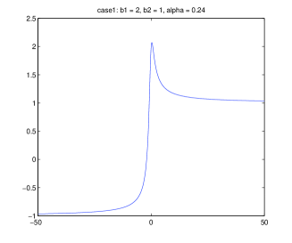
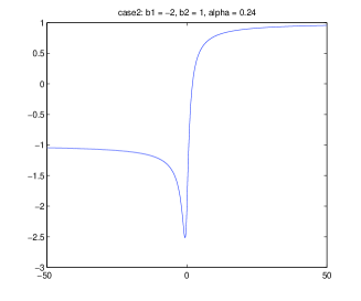
Figure 1: Graph of g(t)

Remark: Assuming $b_{1}\neq 0$, $f(s)$ can be rewritten as following by replacing $s$ as $s=\frac{b_{2}-\alpha b_{1}}{b_{1}-\alpha b_{2}}$.

$$f(s)=\displaystyle\frac{|b_{1}+sb_{2}|}{\sqrt{1+2\alpha s+s^{2}}}=\displaystyle\frac{\sqrt{1-2\alpha r+r^{2}}}{\sqrt{1-\alpha^{2}}}|b_{1}|=|b_{1}|\sqrt{1+\displaystyle\frac{(r-\alpha)^{2}}{1-\alpha^{2}}}$$ (10)

where $r=b_{2}/b_{1}$.

In view of (10), $f(s)\rightarrow\infty$ when $\alpha\rightarrow 1$ (assuming $r$ independent of $\alpha$). It is thus attempting for us to get the next projection $p_{1}$ of $x$ with much bigger length(and thus hopefully more closer to $x$) by carefully selecting suitable vector $d$ with $d^{T}x=b_{2}$ and $\alpha=p_{0}^{T}*d$ is as close as possible to $1$(i.e., the angle between $p_{0}$ and $d$ should be very small). However this seems to be very hard and thus we turn to an easier scheme to fulfill our task—we will use subspaces on which projections of $x$ are easily available. For this purpose we now generalize our conclusion in Lemma 3.1 into following statement.

Lemma 3.2

Let $x,v_{i}\in R^{n}\,(i=1,2,\cdots,m)$, and $W=span\{v_{1},v_{2},\cdots,v_{m}\}$. Let $P_{W}(x)$ be the projection of $x$ onto subspace $W$. Then

$$\frac{v_{*}^{T}x}{||v_{*}||}=\displaystyle\max_{v\in W}\frac{|x^{T}v|}{||v||}$$

where $v_{*}=P_{W}(x)$.

Proof. Without loss of generality we can assume $||x||=1$. By definition of angles between vectors we have

$$f(v)=\frac{|x^{T}v|}{||v||}=\frac{|x^{T}v|}{||v||||x||}=|\cos<x,v>|$$

where $<x,v>$ denotes the angle between vector $x$ and $v$. Obviously $f(v)$ reaches its maximum value if and only if $<x,v>$ is minimized, which is true only when $v$ lies on the projection of $x$ onto subspace $W$.

By using this result, one can always expect a searching direction $d$ on which vector $x$ has a bigger projection length $||P_{d}(x)||$ than any vector in subspace $W=span\{v_{1},v_{2},\cdots,v_{m}\}$ with $x^{T}v_{i}\,(i=1,2,\cdots,m)$ given. Since we have $n$ vectors $a_{i}\,(i=1,2,3,\cdots,n)$ to form subspaces of $R^{n}$, this give us plenty of choices when it comes to construct subspaces. More importantly we can use parallel process to construct these subspaces and figure out projections of $x$ on each of them. Instead of using successive “partial” projections which did not adequately make use of current system information, all these projections of $x$ can be used to construct a better approximation to the current system.

3.2 The projection algorithms

In this subsection we present some basic algorithms for solving linear system of equations. We first introduce two algorithms for calculating a projection vector $p$ of $x$ to the system (1) based on current system data, i.e., the coefficient matrix $A$ and right-hand side vector $b$, which is always the unique vector in some subspace of $R^{n}$ on which solution vector $x$ having the maximum projection length.

In preparation, we begin with the division of all row vectors of $A$ into groups of vectors $\{G_{i}\}_{1}^{k}$, with each group $G_{i}$ contains $m_{i}$ vectors, where $m_{i}\,(i=1,\cdots,k)$ are relatively small integers satisfying $m_{i}<m,\,\forall 1\leq i\leq k$. $m$ is a suitable integer so that the QR factorization of matrix $T_{i}$ formed by all vectors in group $G_{i}$ is applicable; in case of sparse coefficient matrix, QS factorization process based on LGO method pengDDM2009 can be used and thus $m$ can be relatively large(say, up to $O(10^{5})$). The right-hand side vector $b$ is divided correspondingly into vectors $b_{i}\,(i=1,\cdots,k)$.

One thing needs to be mentioned here is that we assume two adjacent groups $G_{i}$ and $G_{i+1}$ contain about half of their vectors in common and any row vector in $A$ must lie in at least one of the groups, we will refer this group $\{G_{i}\}$ as an overlapped division of $A$. A non-overlapped division of $A$ means the intersection of any two groups in the division is empty.

The first accumulated projection algorithm uses an overlapped division of $A$ and seeks the projection vector $p_{i}$ of solution $x$ on the range of each group $G_{i}$, i.e., the subspace spanned by all vectors in $G_{i}$. All projection vectors $\{p_{i}\}_{1}^{k}$ are then “glued” together to form a better projection vector of $x$, while the “gluing” process is nothing but another projection of $x$ over subspace $W=span\{p_{1},\cdots,p_{k}\}$. The details comes as follows.

Algorithm 1

(AP version 1) Let $A\in R^{n\times n}$ be nonsingular, $b\in R^{n}$. The following procedure produces a projection(vector) $p$ of solution $x$ to the system $Ax=b$.

• Step 1. Divide matrix $A$ into $k$ blocks: $A=[A_{1}^{T},A_{2}^{T},\cdots,A_{k}^{T}]^{T}$, divide $b$ correspondingly: $b=(b_{1}^{T},b_{2}^{T},\cdots,b_{k}^{T})^{T}$.

• Step 2. For each $i\in\{1,2,\cdots,k-1\}$, compute projection $p_{i}$ of $x$ in $ran(A_{i}^{T},A_{i+1}^{T})$: $p_{i}=G_{i}^{T}(G_{i}G_{i}^{T})^{-1}B_{i}$ and compute scalar $c_{i}=x^{T}p_{i}$ as $c_{i}=B_{i}^{T}(G_{i}G_{i}^{T})^{-1}B_{i},$ where $G_{i}=[A_{i}^{T},A_{i+1}^{T}]^{T}$ and $B_{i}=(b_{i}^{T},b_{i+1}^{T})^{T}$.

• Step 3. Construct matrix $H$ as $H=[p_{1},p_{2},\cdots,p_{k-1}]$ and vector $c^{T}=(c_{1},c_{2},\cdots,c_{k-1})$.

• Step 4. Form a projection $p$ of $x$ over $ran(H)$ and compute scalar $\alpha$ ($=x^{T}p$).

• Step 5. Output $p$ and $\alpha$.

Remark:

The projection process on each group of row vectors can be handled independently and thus good for parallel implementation.

There exists an important relation between $H$,$c$ and solution vector $x$:

$$H^{T}x=c$$

In case the number of groups is too big so that a direct projection over $ran(H)$ is not applicable, one can use a nested version of this algorithm over $H$ to obtain the final projection vector.

Algorithm 1 uses a sequence of projections on the a set of subspaces determined by submatrices of $A$, these projections can be obtained in parallel, which differs itself with those in Karcmarz’s idea. Furthermore, the blocks of matrices are overlapped with each other. One can of course use different strategies when dividing the matrix $A$ into submatrices and $b$ correspondingly. It is easy to see that direction vector $p$ satisfies

$$\frac{x^{T}p}{||p||}\geq\max_{i\in\{1,\cdots,n\}}\frac{a_{i}x}{||a_{i}||}$$

where $a_{i}$ denotes the $i$th row of matrix $A$. However $p$ may not be the best option in general.

Another accumulated projection idea is to use a sequential projection process to get a final projection vector $p$ of $x$. We begin with an initial projection vector $p_{0}$ of $x$ and let it combine with all row vectors in the first group $G_{i}$ to form a subspace $W_{1}$ of $R^{n}$, and then find the projection vector $p_{1}$ of $x$ in $W_{1}$. $p_{1}$ is then used to combine with all row vector in the next group $G_{2}$ to form a subspace $W_{2}$ so that a projection vector $p_{2}$ of $x$ in $W_{2}$ can be obtained. The above process is repeated until all groups are handled so that the final projection vector $p_{k}$ is available. The following algorithm gives the details.

Algorithm 2

(AP version 2) The following procedure produces a projection vector of $x$ to system $Ax=b$.

• Divide matrix $A$ into $k$ blocks: $A=[A_{1}^{T}.A_{2}^{T},\cdots,A_{k}^{T}]^{T}$, divide $b$ correspondingly: $b=(b_{1}^{T},b_{2}^{T},\cdots,b_{k}^{T})^{T}$. Let $p_{0}=\alpha A^{T}b$, $c=\alpha b^{T}b$ where $\alpha=(b^{T}b)/(b^{T}AA^{T}b)$.

• For $i=1$ to $k$
  step 2.1. Construct matrix $W=[p_{i-1},A_{i}^{T}]$ and vector $l=[c,b_{i}^{T}]^{T}$. step 2.2. Compute the projection vector $p_{i}$ of $x$ onto subspace $ran(W)$ and the scalar $c(=x^{T}p)$. step 2.3: Go to next i.

• Output $p_{k}$ and $c$.

It is observed that Algorithm 2 is more effective than Algorithm 1 in terms of the length of final projection vector $p_{k}$. By this reason, we use Algorithm 2 in our numerical experiments(PAP and APAP algorithms). It should be mentioned here that the AP algorithms depicts a successive projection process over subspace $W_{i}=span\{p_{i},v_{1},v_{2},\cdots,v_{m}\}$ ($i=1,\cdots,k$), where $v_{1},v_{2},\cdots,v_{m}$ denotes the row vectors of submatrix $A_{i}$, and $p_{i}=P_{i-1}x$ is the projection of $x$ over subspace $W_{i-1}$ with $p_{0}$ stands for the initial projection vector of $x$. Hence the whole AP process can be written in the matrix form as $p=P_{k}x$ where $P_{i}$ ($i=1,\cdots,k$) represents the projection matrix over subspace $W_{i}$. It is easy to see that $P_{i}$ depends on vector $x$. As a matter of fact, $P_{k}$ has the form

$$P_{k}=H(H^{T}H)^{-1}$$ (11)

where $H=[p_{k-1},V_{k}]$ and $V_{k}=[v_{1},v_{2},\cdots,v_{k}]$, assuming $p_{k-1}\notin span{V}$.

As a straightforward application, Algorithm 1 and 2 can be used to solve the linear system(1) as stated in the next algorithm.

Algorithm 3

(Progressively Accumulated Projection Method–PAP). Let $A\in R^{n\times n}$, $b\in R^{n}$. The following procedure produces an approximation $y$ to the solution $x$ satisfying $Ax=b$.

• Initialize vector $y$ as zero vector.

• While not converged

  • Use algorithm 1 or 2 to get a projection $p$ of $x$ to system $Ax=b$.

  • Update $y$ as $y=y+p$.

  • Update $b$ as $b=b-Ap$.

  • Check convergence condition.

• Output $p$

PAP is based on the principles in section 2, hence the convergence (Theorem 5.1) of this algorithm is straight-forward and its proof is thus omitted. We need to mention here that unlike classical Krylov subspace methods, the AP-type methods proposed here can actually be used to solve any under-determined systems. Also we have to point out that each sweep in step 2 is a projection process with projection matrix $P_{k}$ varies. The following graph shows the comparison of this algorithm at different iterative numbers, and Table 1 gives the needed iterations for a convergent solution under given tolerance, where the coefficient matrix $A$ is chosen as $A=tridiag(-1,2,-1)$ with $A\in R^{100\times 100}$ and the block size is chosen as $20$ when applying algorithm 2 in this case.

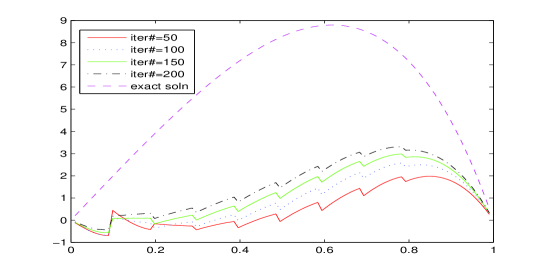
Figure 2: Comparison of approx. solns at different iteration numbers

Table 1: iteration numbers needed for convergence

tolerance	$10^{-1}$	$10^{-2}$	$10^{-3}$	$10^{-4}$	$10^{-5}$	$10^{-6}$	$10^{-7}$
iter#	$3844$	$5534$	$7224$	$8916$	$10606$	$12296$	$13986$

4 Properties of AP process

In this section we present some analysis results for AP process described in Algorithm 2 .

Lemma 4.1

Assume that matrix $A\in R^{m\times n}$ ($m\leq n$) has full row rank, $x\in R^{n}$ and $b\in R^{m}$ where $m\leq n$ satisfying $Ax=b$. Let $A$ be divided into $k$ submatrices by its rows: $A=(A_{1}^{T},A_{2}^{T},\cdots,A_{k}^{T})^{T}$ with $A_{i}\in R^{m_{i}\times n}$, and $b$ is divided as $b=(b_{1}^{T},b_{2}^{T},\cdots,b_{k}^{T})^{T}$ correspondingly. Let $\{p_{i}\}_{1}^{k}$ be the vector sequence produced by AP process(Algorithm 2).

1. There holds for every $i=1,2,\cdots k$

   $$(x-p_{i},p_{s})=0,\quad(s=i,i-1).$$ (12)

2. Vector $p_{i+1}-p_{i}$ ($i=0,1,\cdots,k-1$) is orthogonal to $p_{i}$, i.e.

   $$(p_{i+1}-p_{i},p_{i})=0$$ (13)

3. There holds for $i=1,2,\cdots,k$

   $$||p_{i}||^{2}+||p_{i+1}-p_{i}||^{2}=||p_{i+1}||^{2}$$ (14)

4. For every $s(1\leq s\leq k)$, there holds

   $$||p_{s}||^{2}=||p_{0}||^{2}+\sum_{i=1}^{s}{||p_{i}-p_{i-1}||^{2}}$$ (15)

Proof. (1) We first show that $(x-p_{0},p_{0})=0$. As a matter of fact, since $\alpha=b^{T}b/(b^{T}AA^{T}b)$, we have

$$(x-p_{0},p_{0})=(x-\alpha A_{1}^{T}b_{1},\alpha A^{T}b)=\alpha x^{T}A_{1}^{T}b-\alpha^{2}b^{T}A_{1}A_{1}^{T}b=\alpha b^{T}b-\alpha b^{T}b=0$$

From the fact that $p_{i}$ is the projection of $x$ over subspace $ran(W_{i})$ with $W_{i}=[p_{i-1},A^{T}_{i}]$, for any $i(1\leq i\leq k)$ we must have

$(x-p_{i},p_{i})=0$ and $(x-p_{i},p_{i-1})=0$

since both $p_{i}$ and $p_{i-1}$ belong to $W_{i}$.

(2) Note that from (12) we have

$$(p_{i+1}-p_{i},p_{i})=((x-p_{i})-(x-p_{i+1}),p_{i})=(x-p_{i},p_{i})-(x-p_{i+1},p_{i})=0,$$

which yields (13).

(3) From (13) we have

$$\begin{array}[]{ll}||p_{i+1}-p_{i}||^{2}&=(p_{i+1}-p_{i},p_{i+1}-p_{i})\\ &=(p_{i+1}-p_{i},p_{i+1})\\ &=(p_{i+1},p_{i+1})-(p_{i},p_{i+1})\\ &=(p_{i+1},p_{i+1})-(p_{i},(p_{i+1}-p_{i})+p_{i})\\ &=(p_{i+1},p_{i+1})-(p_{i},p_{i})\\ &=||p_{i+1}||^{2}-||p_{i}||^{2}\end{array}$$

from which (14) comes immediately.

(4) Equation (15) follows from the recursive application of (14):

$$\begin{array}[]{rl}||p_{s}||^{2}&=||p_{s-1}||^{2}+||p_{s}-p_{s-1}||^{2}\\ &=||p_{s-2}||^{2}+||p_{s-1}-p_{s-2}||^{2}+||p_{s}-p_{s-1}||^{2}\\ &\cdots\\ &=||p_{0}||^{2}+||p_{1}-p_{0}||^{2}+||p_{2}-p_{1}||^{2}+\cdots+||p_{s}-p_{s-1}||^{2}.\par\end{array}$$

Proof is completed $\Box$

Lemma 4.1 actually tells the fact that the “length”(norm) sequence $\{||p_{i}||\}_{1}^{k}$ of projection vector $\{p_{i}\}_{1}^{k}$ actually forms a monotonically increasing sequence, and obviously $||x||$ is actually one of its upper bounds. In order to find out how fast this sequence is increasing, we need to figure out the detailed information of each $||p_{i}||\,(i=1,2,\cdots,k)$. The following conclusion answers this question.

Lemma 4.2

Assume the same assumption in Lemma 4.1. Let $\tilde{p}_{i}$ and $\tilde{x}_{i+1}$ be the projection vectors of $p_{i}$ and $x$ over subspace $ran(A_{i+1}^{T})$ respectively. Then $p_{i+1}$ has the following expression

$$p_{i+1}=\alpha_{i}p_{i}+A^{T}_{i+1}u=\alpha_{i}(p_{i}-\tilde{p}_{i})+\tilde{x}_{i+1}$$ (16)

where $u$ is

$$u=\tilde{A}_{i+1}(b_{i+1}-\alpha_{i}A_{i+1}p_{i})$$ (17)

and

$$\alpha_{i}=\frac{x^{T}p_{i}-(A_{i+1}p_{i})^{T}\tilde{A}_{i+1}b_{i+1}}{p_{i}^{T}p_{i}-p_{i}^{T}A_{i+1}^{T}\tilde{A}_{i+1}A_{i+1}p_{i}}=\frac{x^{T}p_{i}-p_{i}^{T}*\tilde{x}_{i+1}}{p_{i}^{T}p_{i}-\tilde{p}^{T}_{i}\tilde{p}_{i}}$$ (18)

and

$$\tilde{A}_{i+1}=(A_{i+1}A_{i+1}^{T})^{-1}.$$

Furthermore

$$||p_{i+1}||^{2}=\alpha_{i}||p_{i}||^{2}+b_{i+1}^{T}\tilde{A}_{i+1}b_{i+1}-\alpha_{i}^{2}(A_{i+1}p_{i})^{T}\tilde{A}_{i+1}(A_{i+1}p_{i})$$ (19)

Proof.
It is valid to express $p_{i+1}$ in the form like the first equation of (16) for some $u\in R^{m_{i+1}}$ since $p_{i+1}\in W_{i+1}=ran([p_{i},A_{i+1}^{T}])$, where $m_{i}$ is the number of rows in submatrix $A_{i}$.

Since $p_{i+1}$ is the projection of $x$ over subspace $W_{i+1}$, we have

$$A_{i+1}(x-p_{i+1})=0$$

which leads to

$$b_{i+1}-\alpha_{i}A_{i+1}p_{i}-A_{i+1}A_{i+1}^{T}u=0$$

from which comes (17). Note that $\tilde{p}_{i}$ and $\tilde{x}_{i+1}$ are projections of $p_{i}$ and $x$ over $ran(A_{i+1}^{T})$, we have

$$\tilde{p}_{i}=A_{i+1}^{T}\tilde{A}_{i+1}A_{i+1}p_{i}\quad\mbox{and}\quad\tilde{x}_{i+1}=A_{i+1}^{T}\tilde{A}_{i+1}b_{i+1}$$ (20)

Plug (17) and (20) back into the first equation of (16) gives the second equation of (16).

Similarly, by $p_{i}^{T}(x-p_{i+1})=0$ we have

$$x^{T}p_{i}-\alpha_{i}p_{i}^{T}p_{i}+u^{T}A_{i+1}p_{i}=0,$$

replacing $u$ by (17) yields the first equation of (18). Again because $\tilde{p}_{i}$ is the projection of $p_{i}$,

$$(p_{i}-\tilde{p}_{i},\tilde{p}_{i})=0,$$

this means

$$p_{i}^{T}\tilde{p}_{i}=\tilde{p}_{i}^{T}\tilde{p}_{i}.$$ (21)

Plug (20) and (21) into the first equation of (18) gives the second equation.

Finally from (16) we have

$$\begin{array}[]{rl}||p_{i+1}||^{2}&=(\alpha_{i}p_{i}+A_{i+1}^{T}u)^{T}(\alpha_{i}p_{i}+A_{i+1}^{T}u)\\ &=\alpha_{i}^{2}p_{i}^{T}p_{i}+2\alpha_{i}p_{i}^{T}A_{i+1}^{T}u+u^{T}A_{i+1}A^{T}_{i+1}u.\\ \end{array}$$ (22)

Since

$$\begin{array}[]{rl}2\alpha_{i}p_{i}^{T}A_{i+1}^{T}u&=2\alpha_{i}p_{i}^{T}A_{i+1}^{T}\tilde{A}_{i+1}(b_{i+1}-\alpha_{i}A_{i+1}^{T}p_{i})\\ &=2\alpha_{i}p_{i}^{T}A_{i+1}^{T}\tilde{A}_{i+1}b_{i+1}-2\alpha_{i}^{2}(A_{i+1}p_{i})^{T}\tilde{A}_{i+1}(A_{i+1}p_{i})\end{array}$$ (23)

and

$$\begin{array}[]{rl}u^{T}A_{i+1}A^{T}_{i+1}u&=(b_{i+1}-\alpha_{i}A_{i+1}p_{i})^{T}\tilde{A}_{i+1}(b_{i+1}-\alpha_{i}A_{i+1}p_{i})\\ &=b_{i+1}^{T}\tilde{A}_{i+1}b_{i+1}-2\alpha_{i}b_{i+1}^{T}\tilde{A}_{i+1}A_{i+1}p_{i}\\ &~{}~{}+\alpha_{i}^{2}(A_{i+1}p_{i})^{T}\tilde{A}_{i+1}(A_{i+1}p_{i}),\\ \end{array}$$ (24)

equation (19) comes from (22) (23) (24) combined. $\Box$

Lemma 4.2 describes one way of constructing $p_{i+1}$, and detailed information about $p_{i+1}$ is revealed by (19). However a more direct approach can be used to evaluate the difference of the norms between two consecutive projections $p_{i+1}$ and $p_{i}$. These can be shown in the following conclusion.

Lemma 4.3

Assume the same assumption in Lemma 4.1. Let $I$ be the identity matrix in $R^{n}$. Then $p_{i+1}$ has the following expression

$$p_{i+1}=p_{i}+\bar{A}_{i+1}^{T}v$$ (25)

and

$$||p_{i+1}||^{2}-||p_{i}||^{2}=(b_{i+1}-(p_{i}^{T}x)d)^{T}(\bar{A}_{i+1}\bar{A}_{i+1}^{T})^{-1}(b_{i+1}-(p_{i}^{T}x)d)$$ (26)

where $\bar{A}_{i+1}$ is a rank-one modification of submatrix $A_{i+1}$ as

$$\bar{A}_{i+1}=A_{i+1}-dp_{i}^{T}=A_{i+1}(I-u_{i}u_{i}^{T})$$ (27)

with $u_{i}=p_{i}/||p_{i}||$, $d\in R^{m_{i+1}}$ a vector taken as $d=A_{i+1}p_{i+1}/||p_{i}||^{2}$ and $v$ is defined as

$$v=(\bar{A}_{i+1}\bar{A}_{i+1}^{T})^{-1}(b_{i+1}-(x^{T}p_{i})d)$$

assuming the related inverse exists.

Proof.
Since $p_{i+1}$ is the projection of $x$ over subspace $W_{i+1}=ran([p_{i},A_{i+1}^{T}])$, it can be constructed as follows.

First we modify row vectors in $A_{i+1}$ so that they are orthogonal to vector $p_{i}$, this can be depicted as a rank-one modification to $A_{i+1}$ as

$$\bar{A}_{i+1}=A_{i+1}-dp_{i}^{T},$$

where $d$ can be obtained from the fact that

$$\bar{A}_{i+1}p_{i}=0$$

which leads to

$$A_{i+1}p_{i}-dp_{i}^{T}p_{i}=0,$$

hence

$$d=A_{i+1}p_{i}/(p_{i}^{T}p_{i}),$$

and

$$\bar{A}_{i+1}=A_{i+1}-dp_{i}^{T}=A_{i+1}-A_{i+1}p_{i}p_{i}^{T}/(p_{i}^{T}p_{i})=A_{i+1}(I-u_{i}u_{i}^{T}),$$

where $u_{i}=p_{i}/||p_{i}||$.

Next we calculate the projection vector $\tilde{p}_{i+1}$ of $x$ over $ran(\bar{A}_{i+1})$ as

$$\tilde{p}_{i+1}=\bar{A}_{i+1}^{T}v,$$

where $v$ can be derived from the fact that

$$\bar{A}_{i+1}(x-\tilde{p}_{i+1})=0,$$

which leads to

$$v=(\bar{A}_{i+1}\bar{A}_{i+1}^{T})^{-1}(b_{i+1}-(p_{i}^{T}x)d)$$

assuming $(\bar{A}_{i+1}\bar{A}_{i+1}^{T})^{-1}$ exists.

Since $\tilde{p}_{i+1}=\bar{A}_{i+1}v$ is the projection of $x$ over $ran(\bar{A}_{i+1})$ and $\bar{A}_{i+1}p_{i}=0$, we must have $(p_{i},\tilde{p}_{i+1})=0$. Therefore

$$\begin{array}[]{rl}||p_{i+1}||^{2}-||p_{i}||^{2}&=||\tilde{p}_{i+1}||^{2}\\ &=v^{T}\bar{A}_{i+1}\bar{A}_{i+1}^{T}v\\ &=(b_{i+1}-(p_{i}^{T}x)d)^{T}(\bar{A}_{i+1}\bar{A}_{i+1}^{T})^{-1}(b_{i+1}-(p_{i}^{T}x)d).\end{array}$$

noting that matrix $(\bar{A}_{i+1}\bar{A}_{i+1}^{T})^{-1}$ is symmetric(actually positive definite symmetric). $\Box$.

Remark: It can be shown that the length difference between $p_{i+1}$ and $p_{i}$ can also be written as

$$||p_{i+1}||^{2}-||p_{i}||^{2}=\tilde{x}^{T}G\tilde{x}$$ (28)

where $G=(\bar{A}_{i+1}\bar{A}_{i+1}^{T})^{-1}$ and $\tilde{x}=\bar{x}-(x^{T}u)u$, where $\bar{x}$ denotes the projection of $x$ on $ran(A^{T})$ and $(x^{T}u)u$ is the projection of $x$ (as well as $\bar{x}$) on the direction of $u=p_{i}/||p_{i}||$.

Note that in the above lemma, we need to assume the existence of each matrix $(\bar{A}_{i+1}\bar{A}_{i+1}^{T})^{-1}$. The following conclusion gives the sufficient and necessary conditions for these to hold true.

Lemma 4.4

Let $A\in R^{m\times n}(m\leq n)$ and $rank(A)=m$, $u\in R^{n}$ be a unit vector in $R^{n}$. Let $\bar{A}=A(I-uu^{T})$ and $G=\bar{A}\bar{A}^{T}$, where $I$ denote the identity matrix in $R^{n}$. Then $G$ is nonsingular if and only if $u\notin ran(A^{T})$.

Proof.
Note that $G=\bar{A}\bar{A}^{T}$ is invertible if and only if $\bar{A}$ is of full row rank.

(Necessity) Assume $G$ is invertible, we need to show that $u\notin ran(A^{T})$. If this is not the case, i.e., $u\in ran(A^{T})$, then there is a $v\in R^{n}$ ( $v\neq 0$) such that $u=A^{T}v$. Thus

$$\bar{A}^{T}v=(A(I-uu^{T}))^{T}v=(A-Auu^{T})^{T}u=A^{T}v-uu^{T}A^{T}v=u-u(u^{T}u)=0$$

since $||u||=1$. This means $\bar{A}$ is not of full rank, hence $G$ is singular, a contradiction with our assumption.

(Sufficiency). Suppose $u\notin ran(A^{T})$, we need to show that $G$ is invertible. As a matter of fact, if $G$ is not invertible, then $\bar{A}$ is not of full-row rank. Therefore there exists a nonzero vector $v\in R^{m}$ such that $\bar{A}^{T}v=0$. That means

$$0=(A(I-uu^{T}))^{T}v=A^{T}v-uu^{T}A^{T}v=A^{T}v-\alpha u$$

where $\alpha=u^{T}(A^{T}v)$ is a scalar. It is easy to see from here that $\alpha\neq 0$, otherwise we would have $A^{T}v=0$ which means $A$ is not of full row rank. Hence $u=A^{T}v/\alpha$, i.e., $u\in ran(A^{T})$, this is contradictory with the assumption. $\Box$

Lemma 4.5

Assume the same assumption in Lemma 4.1. Vector sequence $p_{0}$,$p_{1}$,$\cdots$, $p_{k}$ are produced in one AP process, then

$$||p_{i}||\leq||p_{i+1}||\quad(i=0,1,2,\cdots,k)$$ (29)

and the equal sign holds if and only if

$$A_{i+1}p_{i}=b_{i+1}$$

Proof. Inequality (29) comes from (14) directly. We now prove the necessary condition for $||p_{i+1}||=||p_{i}||$.

(Necessity) Note that if $||p_{i+1}||=||p_{i}||$ holds , by (14) we must have $p_{i+1}=p_{i}$. Also from (16) we know that

$$p_{i+1}=\alpha_{i}p_{i}+A_{i+1}^{T}u,$$

thus

$$A_{i+1}^{T}u=p_{i+1}-\alpha_{i}p_{i}=(1-\alpha_{i})p_{i}.$$ (30)

Multiplying both sides of (30) by $A_{i+1}$ we have

$$A_{i+1}A_{i+1}^{T}u=(1-\alpha_{i})Ap_{i}.$$ (31)

Note that from (17) we have

$$A_{i+1}A_{i+1}^{T}u=b_{i+1}-\alpha_{i}Ap_{i}.$$ (32)

Combining (31) and (32) yields

$$Ap_{i}=b_{i+1}.$$

(Sufficiency)Now we prove $p_{i+1}=p_{i}$ under the assumption $Ap_{i}=b_{i+1}.$

As a matter of fact, in view of (17) and (18) we only need to show that

$$\alpha_{i}=1$$

in this case.

Since $(x-p_{i},p_{i})=0,$ we have

$$x^{T}p_{i}=p_{i}^{T}p_{i}.$$ (33)

By using $A_{i+1}p_{i}=b_{i+1}$ we obtain

$$p_{i}^{T}A_{i+1}^{T}\tilde{A}_{i+1}A_{i+1}p_{i}=b_{i+1}\tilde{A}_{i+1}b_{i+1}$$ (34)

Hence from (18) we have

$$\alpha_{i}=\frac{x^{T}p_{i}-(A_{i+1}p_{i})^{T}\tilde{A}_{i+1}b_{i+1}}{p_{i}^{T}p_{i}-p_{i}^{T}A_{i+1}^{T}\tilde{A}_{i+1}A_{i+1}p_{i}}=\frac{p_{i}^{T}p_{i}-b_{i+1}^{T}\tilde{A}_{i+1}b_{i+1}}{p_{i}^{T}p_{i}-b_{i+1}^{T}\tilde{A}_{i+1}b_{i+1}}=1$$

This completes the proof of the sufficient condition. $\Box$

5 An Accelerative Scheme

We have observed from the preceding sections that the convergence speed of the simple iterative algorithm may not be very satisfactory in general. In this section we are to design some accelerative approach for the PAP algorithm.

If we check the PAP procedure (Algorithm 3) carefully and let $p_{i},c_{i}$ denote the output from each call to algorithm 1 or 2, the sum of $p_{i}$ is used in Algorithm 3 as an approximation $x_{k}$, i.e., $x_{k}=p_{1}+p_{2}+\cdots+p_{k}$ when the $x_{k}$ satisfies some convergence conditions, it is used as the final output approximation. The following facts are obvious.

Theorem 5.1

Let $x_{k}$ be defined as above, $e_{k}=x-x_{k}$, then

$$\lim_{k\rightarrow\infty}x_{k}=x$$

i.e.,

$$\lim_{k\rightarrow\infty}e_{k}=\lim_{k\rightarrow\infty}x-x_{k}=0.$$

and $\{||e_{k}||\}_{1}^{\infty}$ is strictly decreasing.

We aim to use a combination of some selected approximate solution from the sequence $\{x_{k}\}_{1}^{M}$ ( $M\!<\!\infty$) to obtain an “optimal” approximation, named as $y_{1}$, and then use it to update the original system. This process is repeated to get next optimal approximation solution $y_{2}$, and so on and so forth.

In Krylov subspace methods, this can be accomplished by using coefficients of some specially chosen polynomials, as explicitly done in Chebyshev semi-iterative method for accelerating stationary methods or implicitly done in GMRES, FOM, etc. The drawbacks of these techniques are: the resulted combination still falls into a Krylov subspace with the same fixed generator matrix and starting vector, which leads to their ultimate inefficiency in solving large scale problems and thus have to resort to some preconditioning techniques. Furthermore this treatment can not always guarantee a convergent scheme.

Our strategy here is to pick up a subsequence of $\{x_{k}\}_{1}^{M}$, say, starting from an initial $x_{k_{0}}$ in $\{x_{k}\}_{1}^{M}$ and then pick another vector $x_{k_{i}}$ after every $t$ iterations to form a sequence $\{x_{k_{i}}\}_{i=0}^{m}$ with $m$ a small integer. For example, in the sequence $\{x_{k}\}_{1}^{M}$ we pick up $x_{10},x_{20},\cdots,x_{m*10}$ as the subsequence, renamed as $\{v_{k}\}_{1}^{m}$ and then we try to find the projection of $x$ on the subspace $W=span\{v_{1},v_{2},\cdots,v_{m}\}$. To reach this goal we have to resolve two key problems: first one should be able to obtain the inner product between $x$ and each $x_{k}$; secondly one should be able to selectively store the wanted subsequence $\{v_{k}\}_{1}^{m}$ from the sequence $\{x_{k}\}_{1}^{M}$ and discard the unwanted vectors in the sequence without affecting the calculation of inner product between $x$ and $x_{k}$.

The following conclusion helps to resolve these questions.

Theorem 5.2

Let $x$ be the solution to system (1), $r_{0}=b$, $p_{k}$ be the approximation to $e_{k-1}$ in system $Ae_{k-1}=r_{k}$ by Algorithm 1 or 2, $c_{k}=e_{k-1}^{T}p_{k}$ with $e_{-1}=x$, $r_{k}=r_{k-1}-Ap_{k-1}$, $e_{k}=e_{k-1}-p_{k}$, $x_{k}=\sum^{k}_{i=0}p_{i}$. Then

$$x =x_{k}+e_{k},$$ (35)

$$x^{T}p_{k} =c_{k}+x^{T}_{k-1}p_{k}$$ (36)

$$x^{T}x_{k} =\sum^{k}_{i=0}c_{i}+\sum^{k}_{i=0}x_{i-1}p_{i}$$ (37)

for $k=0,1,2,\cdots$.

Proof. Since $e_{i}=e_{i-1}-p_{i}$, we have

$$e_{i-1}=e_{i}+p_{i}.$$

Hence

$$\sum_{i=0}^{k}e_{i-1}=\sum_{i=0}^{k}e_{i}+\sum_{i=0}^{k}p_{i},$$

which can be rewritten as

$$\sum_{i=0}^{k}e_{i-1}-\sum_{i=0}^{k}e_{i}=\sum_{i=0}^{k}p_{i}.$$

Note that $e_{-1}=x$, we have

$$x_{k}=\sum_{i=0}^{k}p_{i}=\sum_{i=0}^{k}e_{i-1}-\sum_{i=0}^{k}e_{i}=e_{-1}-e_{k}=x-e_{k}.$$

Thus

$$x=e_{k}+p_{k},$$

which gives (35).

Note that

$$x^{T}p_{k}=(x_{k-1}+e_{k-1})^{T}p_{k}\\ =x^{T}_{k-1}p_{k}+e^{T}_{k-1}p_{k}\\ =c_{k}+x_{k-1}^{T}p_{k}$$

which yields (36). Finally by (36) we have

$$\begin{array}[]{l}x^{T}x_{k}=x^{T}\sum_{0}^{k}p_{i}=\sum_{0}^{k}x^{T}p_{i}=\sum_{0}^{k}(c_{i}+x_{i-1}^{T}p_{i})=\sum_{0}^{k}c_{i}+\sum_{0}^{k}x_{i-1}^{T}p_{i}\end{array}$$

which gives (37). $\Box$

Expression (37) suggests us that the inner produce between $x$ and $x_{k}$ for any $k$ only depends on two real number sequences $\{c_{i}\}_{0}^{k}$ and $\{\tau_{i}\}_{0}^{k}$ with $\tau_{i}=x_{i-1}^{T}p_{i}$ and $\tau_{i}$ only depends on the last approximation $p_{i}$ to error vector $e_{i}$ and accumulated approximation $x_{i-1}$. Hence it is possible for us to design an algorithm which only needs to store a constantly updating vector $x_{k}$ and save two number sequences $\{c_{i}\}$ and $\{\tau_{i}\}$ during the iteration process. It is thus viable for us to selectively store the wanted approximation $x_{k}$ and discard those unwanted ones in the approximation sequence $\{x_{i}\}_{1}^{M}$.

The following algorithm makes use of these benefits and constantly seeks a projection vector on the subspace formed by the selected approximation vectors.

Algorithm 4

(Accelerated Progressively Accumulated Projection–APAP) Let $x$ be the solution to system (1), $\Delta\subset\{1,2,\cdots,M\}$ be a predetermined index set. The following procedure produces an approximation to the solution $x$ in $Ax=b$.
Step 1: (Initializing) Set $y\in R^{n}$ as zero vector Step 2: Do while not convergent step 2.1 Set $r=b(\in R^{n})$, $l_{i}=0(\in R)$, $x_{i}=0\,(\in R^{n})$ step 2.2 For $i=1$ to $M$ step 2.2.1 Call Algorithm 1 or 2 to get projection vector $p_{i}$ to $e_{i-1}$ satisfying $Ae_{i-1}=r$ and $c_{i}=e_{i-1}^{T}p_{i}$. step 2.2.2 Set $\tau_{i}=x_{i}^{T}p_{i}$, $l_{i}=l_{i}+\tau_{i}+c_{i}$ step 2.2.3 Set $x_{i}=x_{i}+p_{i}$ step 2.2.4 Update $r$ as $r=r-Ax_{i}$. step 2.2.5 Store $x_{i}$ into matrix $H$ as a row vector and $l_{i}$ into vector $L$ if $i\in\Delta$. step 2.3 Calculate projection vector $v$ of $\bar{x}(=A^{-1}b)$ on $ran\{H\}$ $$v=H(H^{T}H)^{-1}L$$ step 2.4 $y=y+v$ step 2.5 $b=b-Av$ end

Remark:

In both PAP and APAP methods one has to repeatedly call basic AP methods(version 1 or version 2) to get the projections. Hence in actual implementation of these two algorithms it is necessary to rewrite the original system into its equivalent forms. In case the division of $A$ and $b$ is non-overlapped, each subsystem $A_{i}x=b_{i}$ corresponding to the division can be rewritten as $Q_{i}^{T}x=\tilde{b}_{i}$ where $Q_{i}R_{i}=A_{i}^{T}$ forms the QR factorization(in case $A$ is dense) or QS factorization(in case $A$ is sparse) of $A_{i}$, while $\tilde{b}_{i}=(R_{i}^{T})^{-1}b_{i}$; in case of an overlapped division, one can use some extra sequence of submatrix-vector pairs to get the projections easily. By these rearrangement it is thus very efficient for us to get the projections of any vector on each subspaces. Note that the orthogonalization of each submatrix is needed only once.

It turns out that the accelerating effect of this algorithm is remarkable by comparing Table 1 and Table 2 where the block sizes in both tests are exactly the same and the predetermined index set is selected as $\Delta=\{10,20,30,40,50,60\}$. For instance, to reach the same level $O(10^{-7})$ of relative residual error, PAP method(Algorithm 3) needs almost 14000 iterations while APAP method(Algorithm 4) needs only $2\times 60=120$ iterations, an amazingly improved convergence speed!

Table 2: iteration numbers needed for convergence using APAP

tolerance range	$10^{-1}$ – $10^{-7}$	$10^{-8}$–$10^{-13}$	$10^{-14}$–$10^{-19}$
outter iter#	$2$	$3$	$4$

6 Numerical Experiments

In this section we will show some applications of the aforementioned APAP method. APAP is used to compare with block Jacobi method and GMRES since both are currently benchmark iterative methods in the category of extended Krylov subspace methods: the former is stationary and the later is non-stationary.

In the first example, we chose coefficient matrix $A\in R^{400\times 400}$ as the following tridiagonal matrix

$$A=tridiag(-1,2,-1)$$

and the solution vector $x$ is taken as the values of function $u(t)=t(1-t)e^{3+t}$ at grid points $t=i\cdot h$ ($i=1,2,\cdots,400$) and $h=1/401$. The results are listed in Table 3.

Table 3: Comparison between APAP and block Jacobi

block size	cpu time(s)		iter #		rel. residual
	blk Jacobi	apap	blk Jacobi	apap	blk Jacobi	apap
30	34.9	2.70	11015	540	4.03e-5	1.59e-9
35	26.8	2.31	9528	440	3.73e-5	5.52e-11
40	20.2	1.60	8406	330	3.49e-5	1.38e-10
45	18.2	1.08	7533	220	3.29e-5	6.67e-10
50	16.4	1.36	6827	320	3.12e-5	4.27e-11

We can see from this table that APAP exhibits much better performance than block Jacobi method does in terms of precision measured by the relative residuals, in the mean time APAP used much less cpu time and iteration numbers either.

As the second example, we use APAP to solve the Poisson problem defined on the unit square $[0,1]\times[0,1]$. The discretization scheme is the FDM five-point stencil, the resulted coefficient matrix $A$ is a symmetric block diagonal matrix $A\in R^{n\times n}$ ($n=2000$) and the exact solution $u\in R^{n}$ is taken as grid values of function $u=x(1-x)y(1-y)e^{3+x^{2}+y^{2}}$ at grid nodes $\{(i\cdot hx,j\cdot hy)\}$ with $i=1,\cdots,50,j=1,\cdots,40$ and $hx=1/51,hy=1/41$. The following table shows the iterations need for convergence with tolerance set as $10^{-5}$ as well as the comparison between the relative errors obtained by these two methods. Note that here the matrix $A$ has a relatively small condition number $cond(A)=867$ and the block size is determined as $\sqrt{mn}$ so that an AP iteration needs approximately the same amount of storage as those of GMRES, where $n$ is the size of the system and $m$ is the predetermined restart number for $GMRES(m)$, note that the actual iteration number of $GMRES(m)$ is $out*in$ with $out$ as the specified maximum iteration for GMRES and $in$ as the restart number Matlab actually used in its running, while the actual iteration number is also counted as $out*in$. It seems that GMRES outperforms APAP in terms of time and iteration numbers in this case. We also need to mention here since the coefficient matrix $A$ is SPD, thus CG can be used to solve this problem and we recorded that CG outperforms both GMRES and APAP in this example in both cpu time and accuracy.

Table 4: Comparison between APAP and GMRES

settings		iter. #		time(in s)		rel. error
apap	gmres	apap	gmres	apap	gmres	apap	gmres
blk_size	restart	(out,in)	(out,in)
90	4	(12,50)	(234,1)	13.3	8.4	7.6e-5	1.6e-4
110	6	(8,50)	(106,3)	9	2.7	2.5e-5	1.6e-4
127	8	(4,50)	(61,3 )	4.6	3.9	7.5e-5	1.6e-4
142	10	(4,50)	(40,4 )	4.6	3.2	6.5e-5	1.6e-4
155	12	(3,50)	(28,11)	4.1	3.1	7.6e-5	1.5e-5
168	14	(3,50)	(22,2 )	4.1	2.9	3.7.e-5	1.5e-5
179	16	(3,50)	(17,11 )	4.1	2.5	5.1e-5	1.5e-5
190	18	(2,50)	(14,13)	3.0	3.4	5.2e-6	1.4e-5

The third test is on a system with asymmetric coefficient matrix

$$A=tridiag(-1,2,-1.05)$$

having condition numbers varying from $18944$ to $4.0902*10^{51}$ with $n$ varying from $100$ to $4600$, the following table shows the comparison between APAP and GMRES applied on the same systems with exact solution as $u=2\sin(\pi x)e^{3+x}$. Note that the iteration number for APAP and GMRES are the total iteration numbers computed as inner loop multiplied by outer loop numbers. The restart number ($m$) for GMRES is fixed at $8$. It is interesting to see that the relative error of APAP is much better than that of GMRES, different than that in the second example.

Table 5: Comparison between APAP and GMRES

apap	iter. #		time(in s)		rel. error		rel. residual
size	gmres	apap	gmres	apap	gmres	apap	gmres	apap
29	8.0e+3	729	1.4	0.14	3.14e-2	6.71e-8	4.84e-4	1.37e-6
70	4.8e+4	2016	10.3	0.95	8.19e-4	2.33e-4	2.33e-4	7.60e-6
94	8.8e+4	456	27.5	0.90	3.2e-4	9.68e-5	9.10e-5	1.24e-7
114	1.28e+5	309	42.3	1.66	1.81e-4	5.59e-5	5.14e-5	6.41e-6
130	1.68e+5	309	69.8	2.78	1.20e-4	3.74e-5	3.40e-5	6.98e-7
145	2.08e+5	309	135.1	5.52	8.69e-5	2.72e-5	2.46e-5	2.40e-7
158	2.48e+5	309	296.8	7.47	6.66e-5	2.10e-5	1.88e-5	8.07e-8
170	2.88e+5	309	342.7	11.18	5.32e-5	1.68e-5	1.50e-5	1.80e-8
182	3.28e+5	309	400.6	11.52	4.37e-5	1.38e-5	1.24e-5	7.41e-9
192	3.68e+5	309	417.7	13.40	3.67e-5	1.16e-5	1.04e-5	4.86e-9

As the last experiment we use Hilbert matrix as the coefficient matrix $A$ in system (1), the solution $x$ is exactly as in example 2.

Hilbert matrix is a well-known extremely ill-conditioned matrix and its condition number grows exponentially. In our experiments the direct solver in the MATLAB math package will fail to produce any significant solution to system (1) as $n$ is greater than $16$. However by using APAP we can solve this system with $n$ up to a few thousand in this case(see figure 3). Again in this case CG can be applied and it takes much less cpu time to reach the same accuracy;

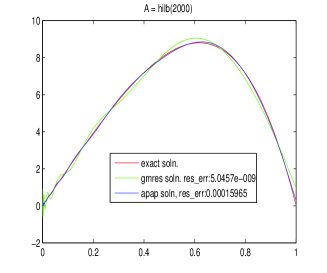
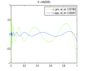
Figure 3: Comparison of approx. solns between GMRES and APAP

It is interesting to notice here that although the approximate solution given by GMRES yields a much better relative residual, its relative error is a little worse than that of approximate solution given by APAP.

7 Comments and Summary

In this paper we discussed a new type of projection methods with the newly introduced AP technique. The major features of these type of iterative methods which make them differ from current existing prevalent Krylov subspace methods includes: (1) the inner products between each approximate solution and the exact solution is recorded and used for later approximations; (2) they are the first type of non-Krylov subspace methods as far as authors know; (3) the AP techniques actually help to expand the original system into a much larger size of systems (i.e., many more equations can be embedded into the original system with the same solution) and therefore bring much more opportunity for designing accelerative schemes like the one in APAP method.

These type of methods can overcome some shortcomings of current prevailing Krylov subspace methods and exhibit better performance in many of our test problems, especially in case of large sparse linear systems. We have to point out that the construction of some test systems are made so that the exact solutions have dominant components coming from the eigenvalues of the coefficient matrix $A$ with smallest eigenvalues in magnitude, and our test shows that Krylov subspaces usually have a slow convergence speed in these situations, while the APAP method introduced here has a much stable and better performance behavior. APAP can also be used to solve systems with dense coefficient matrices, however to make it applicable, one needs an efficient process to get the projection vectors of $x$ into subspaces formed by row vectors of submatrices of the coefficient matrix, which will be introduced in our later work. When the size of the blocks decreases, or equivalently the number of blocks increases, the convergence speed deteriorate. A remedy is to simply increase the number of AP sweep in each AP process and our numerical experiments show that the time cost is quite reasonable. Currently there is no theoretical results for predicting the iteration numbers needed for any specified tolerance level, since it depends on detailed error analysis of AP process, which seems to be a challenging problem since there does not exist a so-called iteration matrix in the above AP schemes as those in traditional iterative schemes.

References

- [1] O. Axelsson. A survey of preconditioned iterative methods for linear systems of equationns. BIT, 25:166–187, 1985.
- [2] O. Axelsson. Iterative Solution Methods. Cambridge University Press, 1994.
- [3] R. Barrett, M. Berry, T. F. Chan, J. Demmel, J. Donato, J. Dongarra, V. Eijkhout, R. Pozo, C. Romine, and H. Van der Vorst. Templates for the Solution of Linear Systems: Building Blocks for Iterative Methods, 2nd Edition. SIAM, Philadelphia, PA, 1994.
- [4] M. Benzi. Preconditioning techniques for large linear systems: A survey. Journal of Computational Physics, 182:418–477, 2002.
- [5] R. Bramley and A. Sameh. Row projection methods for large nonsymmetric linear systems. SIAM J. on Scientific Computing, 13(1), 1992.
- [6] G. Cimmino. Calcolo approssimato per le soluzioni dei sistemi di equazioni lineari. Ric. Sci. Progr. tecn. econom. naz., 9:326–333, 1939.
- [7] B.N. Datta. Numerical Linear Algebra and Applications. Brooks/Cole Publishing Company, Pacific Grove, 1995.
- [8] J. W. Demmel, J. R. Gilbert, and X. S. Li. An asynchronous parallel supernodal algorithm for sparse gaussian elimination. SIAM J. Matrix Analysis and Applications, 20(4):915–952, 1999.
- [9] I. S. Duff. Direct methods for solving sparse systems of linear equations. SIAM J. Sci. Stat. Comput., 5:605–619, 1984.
- [10] I.S. Duff. Sparse numerical linear algebra: direct methods and preconditioning. In I.S. Duff and G.A. Watson, editors, The State of the Art in Numerical Analysis, pages 27–62. Oxford University Press, 1997.
- [11] R.W. Freund and N. M. Nachtigal. Qmr: A quassi-minimal residual method for non-herminian linear systems. Numeri. Math., pages 315–339, 1991.
- [12] A. Galántai. Projectors and Projection Methods. Springer Sciences + Business Media LLC, 2004.
- [13] A. George. Nested dissection of a regular finite element mesh. SIAM Journal on Nuerical Analysis, 10:345–363, 1973.
- [14] G. H. Golub and C. F. Van Loan. Matrix Computations. The Johns Hopkins University Press, Baltimore and London, 1996.
- [15] W. Hackbusch. Multi-Grid Methods and Applications. Springer-Verlag, Berlin, 1985.
- [16] W. Hackbusch. Iterative Solution of Large Sparse Systems of Equations. Springer-Verlag, New York, 1994.
- [17] C. C. Paige and M.A. Saunders. Solution of sparse indefinite systems of linear equations. SIAM J. Numer. Anal., pages 617–629, 1975.
- [18] W. Peng. A lgo-based elimination solver for large scale linear system of equations. Numerical Mathematics– A Journal of Chinese Universities, 36(2):159–166, 2014.
- [19] W. Peng and B. N. Datta. A sparse qs-decomposition for large sparse linear system of equations. In Y. Huang et al., editor, Domain Decomposition Methods in Science and Engineering XIX, Lecture Notes in Computational Science and Engineering, volume 78, pages 431–438. Spring-Verlag, 2011.
- [20] Y. Saad. Iterative methods for sparse linear systems (2nd ed.). SIAM., 2003.
- [21] Y. Saad and M. Schultz. Gmres: A generalized minimal residual algorithms for solving nonsymmetric linear systems. SIAM J.Scientific and Stat. Comp., pages 856–869, 1986.
- [22] R.S Varga. Matrix Iterative Analysis. Prentice-Hall, Englewood Cliffs, NJ, 1962.
- [23] Henk A. Van Der Vorst. Bicgstab: A fast and smoothly converging varient of the bi-cg for the solution of nonsymmetric linear systems,. SIAM J. Sci. and Stat. Comp., pages 631–644, 1992.
- [24] Henk A. Van Der Vorst. Iterative Krylov Methods for Large Linear Systems. Cambridge University Press, 2003.
- [25] D. M. Young. Iterative Solution of Large Linear Systems. Academic Press, New York, 1971.