On horizons and wormholes in k-essence theories

K. A. Bronnikov,^a,b,c,1 J. C. Fabris,^c,d,2 and D. C. Rodrigues^d

^a

VNIIMS, Ozyornaya ul. 46, Moscow 119361, Russia

^b

Institute of Gravitation and Cosmology, PFUR, ul. Miklukho-Maklaya 6, Moscow 117198, Russia

^c

National Research Nuclear University “MEPhI”, Kashirskoe sh. 31, Moscow 115409, Russia

^d

Universidade Federal do Espírito Santo, Vitória, ES, CEP29075-910, Brazil

We study the properties of possible static, spherically symmetric configurations in k-essence theories with the Lagrangian functions of the form $F(X)$, $X\equiv\phi_{,\alpha}\phi^{,\alpha}$. A no-go theorem has been proved, claiming that a possible black-hole-like Killing horizon of finite radius cannot exist if the function $F(X)$ is required to have a finite derivative $dF/dX$. Two exact solutions are obtained for special cases of k-essence: one for $F(X)=F_{0}X^{1/3}$, another for $F(X)=F_{0}|X|^{1/2}-2\Lambda$, where $F_{0}$ and $\Lambda$ are constants. Both solutions contain horizons, are not asymptotically flat, and provide illustrations for the obtained no-go theorem. The first solution may be interpreted as describing a black hole in an asymptotically singular space-time, while in the second solution two horizons of infinite area are connected by a wormhole.

1 Introduction

A great number of modifications and extensions of the century-old general relativity (GR) theory have been proposed since its formulation in 1915, and, which is surprising and remarkable, they are continuing to emerge nowadays. Such new proposals are motivated by many reasons, among them are the old problem of unifying gravity with other physical interactions and the difficulties in attempts to quantize GR. One should also mention two main problems concerning classical GR itself: the existence of singularities in the most physically relevant solutions of GR, and the necessity to introduce unknown forms of matter in order to explain the main features of the observed universe. The modifications evoked in the literature can be divided into two large classes. In the first one, the geometric sector is generalized: it includes, in particular, $f(R)$ thories, multidimensional theories and non-Riemannian geometries. The second class involves new fundamental, non-geometric fields with nonstandard structure. To the second class one may attribute scalar-tensor theories, Galileons and Horndesky theories and others. It is frequently possible to establish a connection between the two approaches.

The k-essence theories [1] evidently belong to those with nonstandard fundamental fields coupled to gravity. This class is based on a possible non-standard form of the kinetic term of a scalar field. It was for the first time suggested in [2] in order to have an inflationary model driven by the kinetic term instead of the potential. But soon after this idea was applied to explain the present stage of accelerated expansion of the Universe [3]. It is interesting to note that a k-essence structure also appears in string theories as, for example, in the Dirac-Born-Infeld action, where the kinetic term of the scalar field has a structure similar to the Maxwell-like term in Born-Infeld electrodynamics [4].

The k-essence theories can be defined by the following most general Lagrangian:

$${}{\cal L}=\sqrt{-g}[R-F(X,\phi)],$$ (1)

with

$$X=\eta\phi_{;\rho}\phi^{;\rho},$$ (2)

where $\eta=\pm 1$ can be used to make $X$ positive in the cases like general power-law dependence, ill-defined for negative quantities. There are other, more special presentations of k-essence Lagrangians, for example,

$${\cal L}=\sqrt{-g}[R-f(X)+2V(\phi)],$$ (3)

separating the kinetic and potential terms.

While many studies have been carried out in the context of cosmology for k-essence theories, a much smaller effort was applied to study the possible effect of k-essence on the structure and properties of local objects, like, for instance, black holes and wormholes. The aim of this paper is to consider possible static, spherically symmetric configurations in theories defined by the Lagrangian (1).

Although the field equations are written in full generality for the Lagrangian (1) (Section 2), the results obtained here actually concern the more specific form (3). The complexity of the equations prevents us to find more or less general explicit solutions. However, it has been possible to prove a general no-go theorem which states that, in the absence of a $\phi$-dependent potential term in (3), only horizons inherent to cold black holes [5, 6] can appear in these theories, similarly to what happens in scalar-tensor theories (Section 3). A cold black hole is a term coined in [5, 6] to designate asymptotically flat static spherical solutions where the horizon surface is infinite. The surface gravity of such black holes is zero, implying a zero Hawking temperature. However, the tidal forces acting on extended test bodies are infinite at the horizon. It turns out that in scalar-tensor theories like the Brans-Dicke theory, in the absence of a potential term in the Lagrangian, the scalar-vacuum solutions in general contain naked singularities and, in some special cases, cold black hole solutions are possible. We will show that, again in the absence of a potential, only cold black hole horizons are possible in k-essence theories.

Further on we obtain two special exact solutions, one for $V=0$ and $f(X)\sim X^{1/3}$ (Section 4), another for $f(X)\sim|X|^{1/2}$ in the presence of a cosmological constant (Section 5), and briefly describe their properties. Section 6 contains some final remarks.

2 Basic equations

Variation of the Lagrangian (1) with respect to the metric and the scalar field leads to the field equations

$${}G_{\mu}^{\nu}=-T_{\mu}^{\nu}[\phi],$$ (4)

$${}T_{\mu}^{\nu}[\phi]\equiv\eta F_{X}\phi_{\mu}\phi^{\nu}-\frac{1}{2}\delta_{\mu}^{\nu}F,$$ (5)

$${}\eta\nabla_{\alpha}(F_{X}\phi^{\alpha})-{{\displaystyle\frac{1}{2}}}\,F_{\phi}=0,$$ (6)

where $G_{\mu}^{\nu}$ is the Einstein tensor, $F_{X}=\partial F/\partial X$, $F_{\phi}=\partial F/\partial\phi$, and $\phi_{\mu}=\partial_{\mu}\phi$.

Now, consider a general static, spherically symmetric metric

$$ds^{2}=e^{2\gamma(u)}dt^{2}-e^{2\alpha(u)}du^{2}-e^{2\beta(u)}d\Omega^{2}$$ (7)

($d\Omega^{2}=d\theta^{2}+\sin^{2}\theta d\varphi^{2}$ is the metric on a unit sphere) with an arbitrary radial coordinate $u$, and $\phi=\phi(u)$. Then, in the general case (1), the stress-energy tensor (SET) $T_{\mu}^{\nu}$ has the following nonzero components:

$${}T^{0}_{0}=T^{2}_{2}=T^{3}_{3}=-F/2,$$

$${}T^{1}_{1}=-F/2-\eta F_{X}e^{-2\alpha}\phi^{\prime 2},$$ (8)

where the prime denotes $d/du$. In the case under consideration, $X=-\eta e^{-2\alpha}\phi^{\prime 2}$, and to make $X$ positive, in what follows we put $\eta=-1$ (unless otherwise indicated).

The scalar field equation and the nontrivial components of the Einstein equations can be written as follows:

$${}2\Big{(}F_{X}e^{-\alpha+2\beta+\gamma}\phi^{\prime}\Big{)}^{\prime}-e^{\alpha+2\beta+\gamma}F_{\phi}=0,$$ (9)

$${}\gamma^{\prime\prime}+\gamma^{\prime}(2\beta^{\prime}+\gamma^{\prime}-\alpha^{\prime})={{\textstyle\frac{1}{2}}}e^{2\alpha}(F-XF_{X}),$$ (10)

$${}-e^{2\alpha-2\beta}+\beta^{\prime\prime}+\beta^{\prime}(2\beta^{\prime}+\gamma^{\prime}-\alpha^{\prime})$$

$${}\hskip 72.26999pt={{\textstyle\frac{1}{2}}}e^{2\alpha}(F-XF_{X}),$$ (11)

$${}-e^{-2\beta}+e^{-2\alpha}\beta^{\prime}(\beta^{\prime}+2\gamma^{\prime})={{\textstyle\frac{1}{2}}}\,F-XF_{X},$$ (12)

where (12) (the component $G^{1}_{1}=\ldots$) is a first integral of the other equations.

In particular, we will use the so-called quasiglobal radial coordinate [8] $u=:x$ specified by the condition $\alpha(u)+\gamma(u)=0$, it is especially convenient for considering Killing horizons which are then described as regular zeros of the function $A(x)=e^{2\gamma}=e^{-2\alpha}$. The metric has the form

$$ds^{2}=A(x)dt^{2}-\frac{dx^{2}}{A(x)}-r^{2}(x)d\Omega^{2}.$$ (13)

In these coordinates, two combinations of Eqs. (10)–(12) take rather a simple form:

$${}2A\,\frac{r^{\prime\prime}}{r}=X\,F_{X},$$ (14)

$${}A^{\prime\prime}r^{2}-A(r^{2})^{\prime\prime}=-2,$$ (15)

where now the primes stand for $d/dx$. The other two equations, (9) and (12), are rewritten as

$${}2(F_{X}\,Ar^{2}\phi^{\prime})^{\prime}-r^{2}F_{\phi}=0,$$ (16)

$${}\frac{1}{r^{2}}(-1+A^{\prime}rr^{\prime}+Ar^{\prime 2})={{\displaystyle\frac{1}{2}}}F-XF_{X}.$$ (17)

Equations (14) and (15) are the combinations $G^{0}_{0}-G^{1}_{1}=\ldots$ and $G^{0}_{0}-G^{2}_{2}=0$. Equation (15) can be once easily integrated:

$$B^{\prime}(x)\equiv\biggl{(}\frac{A}{r^{2}}\biggr{)}^{\prime}=\frac{6m-2x}{r^{4}},$$ (18)

where the constant $m$ has the meaning of the Schwarzschild mass if the metric is asymptotically flat as $x\to\infty$.

An important point connected with Eq. (14) is that it relates the sign of the difference $T^{0}_{0}-T^{1}_{1}=-XF_{X}=\rho+p$ (in the standard perfect-fluid notation) with the quantity $r^{\prime\prime}$ [8]. Namely, if $r^{\prime\prime}<0$, then $T^{0}_{0}-T^{1}_{1}>0$, and the Null Energy Condition (NEC) is fulfilled; on the contrary, if $r^{\prime\prime}>0$, this condition is violated, and, in particular, wormhole throats are possible. It is clear that the general Lagrangian (1) or even (3) make possible any sign of $XF_{X}$ and hence $r^{\prime\prime}$.

3 A no-go theorem

The structure of the SET (2) leads to an important statement about possible horizons in space-times with the metric (7) even in the general case (1) (the Global Structure Theorem) [7]: there can be at most two simple (Schwarzschild-like) horizons at finite radius $r=e^{\beta}$, and no more than one such horizon if the space-time is asymptotically flat. This result directly follows from the equality $T^{0}_{0}=T^{2}_{2}$, leading to Eq. (15) that does not contain any functions of $\phi$.

Indeed, as already mentioned, horizons are described by regular zeros of the function $A(x)$ or, equivalently, $B(x)=A/r^{2}$ (provided that $r$ is finite). Meanwhile, it follows from (15) that the function $B(x)$ cannot have a regular minimum, therefore, once having become negative, $B(x)$ never returns to zero.

There are many other results of interest concerning the possible existence or non-existence of horizons in configurations with scalar fields. Let us mention, for instance, the no-hair theorem by Adler and Pearson [9], claiming that there cannot be asymptotically flat black holes with a nontrivial scalar field in the case $F=X-2V(\phi)$ with $\eta=1$ (a normal, non-phantom scalar field) and nonnegative potentials $V$. It was generalized in [10] to certain multiscalar and multidimensional space-times.

Here we will obtain one more “no-hair” result concerning the important family of Lagrangians (1), those with $F=f(X)$.

With $F=f(X)$, Eq. (9) is integrated giving

$$f_{X}e^{-\alpha+2\beta+\gamma}\phi^{\prime}=C={\rm const},$$ (19)

or, if we again use the quasiglobal coordinate $u=x$,

$$Af_{X}\phi^{\prime}=C/r^{2}.$$ (20)

and Eq. (14) can be rewritten as

$$2\frac{r^{\prime\prime}}{r}=-\phi^{\prime}{}^{2}f_{X}=-\frac{C^{2}}{A^{2}r^{4}f_{X}},$$ (21)

Let us look whether or not the system admits a Killing horizon like event horizons of static black holes. From the above-mentioned Global Structure Theorem [7] it follows that if $A(x)>0$ in some range of $x$ (where the metric is really static), such a horizon can only be first-order, such that the function $A(x)$ behaves as $A\sim x-x_{h}$.

Looking at (20), we see that $A\to 0$ at finite $r$ implies $f_{X}\phi^{\prime}\to\infty$ (excluding the trivial case $C=0$). On the other hand, again due to (20), the expression $Xf_{X}$, which enters into the SET, is equal to $C\phi^{\prime}/r^{2}$. Therefore finiteness of the SET components $T_{\mu}^{\nu}$, necessary for space-time regularity implies $|\phi^{\prime}|<\infty$, hence a horizon requires $f_{X}\to\infty$.

Thus we have obtained the following no-go theorem: The existence of a black-hole-like Killing horizon at finite $r$ is incompatible with a regular function $f(X)$.

Meanwhile, what we have called a cold black hole [5, 6], with a horizon of infinite area ($r=\infty$), still remains possible if $Ar^{2}$ tends to a finite constant.

4 Special solution 1

It happens that Eqs. (9)–(12), or equivalently (14)–(17), are quite hard to solve, even in the comparatively simple case

$$F(X)=F_{0}X^{n},\qquad F_{0},\ n={\rm const}.$$ (22)

To our knowledge, the only thus far existing example of an exact solution is the well-known case of a linear massless scalar field, $n=1$, with Fisher’s solution [11] and its phantom (“anti-Fisher”) counterpart leading to the simplest wormhole solutions [12, 13]. We will give here one more example, with $n=1/3$, which, although looks somewhat exotic, still illustrates the no-go theorem obtained in the previous section and has some features of interest.

Let us use, as before, the quasiglobal coordinate $u=x$, corresponding to the metric (5). Under the assumption (22), Eq. (20) leads to the following expression for $\phi^{\prime}$:

$$\phi^{\prime}=\left[\frac{C}{nF_{0}A^{n}r^{2}}\right]^{1/(2n-1)}.$$ (23)

Substituting it into (14), we obtain

$$2\frac{r^{\prime\prime}}{r}=\biggl{[}(nF_{0})^{-1}A^{1-3n}C^{2n}r^{-4n}\biggr{]}^{1/(2n-1)}.$$ (24)

We see that the function $A(x)$ drops out from this equation in the case $n=1/3$, which then leads to the equation

$$r^{\prime\prime}=3Kr^{5},\qquad 3K:=F_{0}^{3}/(54C^{2}).$$ (25)

whose first integral is

$$r^{\prime 2}=Kr^{6}+K_{1},\qquad K_{1}={\rm const}.$$ (26)

This equation can be further integrated, but with $K_{1}\neq 0$ one obtains very bulky expressions with elliptic integrals which will not be considered. Assuming $K_{1}=0$, we easily obtain without loss of generality

$$r(x)=\frac{1}{k\sqrt{x}},\quad\ k=\sqrt{2\sqrt{K}}=\frac{2^{1/4}}{3}\frac{F_{0}^{3/4}}{\sqrt{|C|}},$$ (27)

where we have suppressed the emerging integration constant by choosing the zero point of $x$. Thus the solution is defined at $x>0$.

From (27) it follows that $r^{\prime\prime}=3/(4kx^{5/2})>0$, it means that the NEC is violated, and our k-essence field is of phantom nature.

It is straightforward to find the expressions for $B(x)$ and $\phi^{\prime}(x)$ from (18) and (23):

$$B(x) = B_{0}+k^{4}\Big{(}2mx^{3}-{{\displaystyle\frac{1}{2}}}x^{4}\Big{)},$$ (28)

$${}\phi^{\prime}(x) = \biggl{(}\frac{F_{0}}{3C}\biggr{)}^{3}Br^{8}.$$ (29)

A further substitution of these quantities to Eq. (17) should verify the correctness of the solution and maybe lead to a relation between its integration constants. Doing so, we find in the left-hand side of (17)

$$G^{1}_{1}=-3k^{2}m+\frac{3B}{4k^{2}x^{3}},$$ (30)

whereas the right-hand side, $-T^{1}_{1}$, contains only the second term of this expression. We conclude that this solution only exists with $m=0$. The resulting metric has the form

$${}ds^{2}=\Big{(}\frac{B_{0}}{k^{2}x}-\frac{k^{2}}{2}x^{3}\Big{)}dt^{2}-\Big{(}\frac{B_{0}}{k^{2}x}-\frac{k^{2}}{2}x^{3}\Big{)}^{-1}dx^{2}$$

$${}\hskip 72.26999pt-\frac{1}{k^{2}x}d\Omega^{2}.$$ (31)

If $B_{0}\leq 0$, the function $A(x)$ is negative, and the metric describes a particular Kantowski-Sachs cosmological model. If $B_{0}>0$, the metric is static at $x<x_{h}=(2B_{0})^{1/4}/k$, has a horizon at $x=x_{h}$ and is cosmological at larger $x$. Although the metric is perfectly regular in the whole range $x\in{\mathbb{R}}_{+}$, the original function $F(X)$ in the Lagrangian is singular at the horizon. Indeed, we easily verify that $F_{X}=(F_{0}/3)X^{-2/3}\propto 1/A^{2}$, it is infinite at a horizon where $A=0$ and $X=0$, in full agreement with the above no-go theorem. But of interest is the very existence of a regular metric in the presence of a singular function $F(X)$ in the Lagrangian.

Another observation of interest is the negative sign of $X=A\phi^{\prime 2}$ in the T-region $x>x_{h}$. The existence and regular behavior of the solution in this region is evidently related to the odd denominator in the exponent 1/3, owing to which we simply have there $F(X)<0$, whereas for general $n$ the power-law function $X^{n}$ is ill-defined.

With any $B_{0}\neq 0$, the metric (4) has singularities both at $x=0$ where $r=\infty$ and at $r=\infty$ where $r=0$: at both ends, the scalar field $\phi$ and the Kretschmnn scalar $R_{\mu\nu\rho\sigma}R^{\mu\nu\rho\sigma}$ tend to infinity. The Carter-Penrose diagram in the case $B_{0}>0$ (Fig. 1) looks like that for de Sitter space-time. However, unlike the latter, the nonstatic T-region here corresponds to smaller radii $r(x)$ than the static region, just as in black hole space-times; in addition, now all sides of the square in the diagram correspond to singulariries. One can conclude that the solution describes a black hole in space-time with a singular asymptotic.

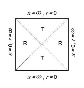
Figure 1: Carter-Penrose diagram for solution 1 with $B_{0}>0$. The letters R and T correspond to static and nonstatic regions, respectively.

5 Special solution 2

Let us now consider the special case of the Lagrangian (3) with

$$F=F(X)=F_{0}X^{n}-2\Lambda,\quad\ F_{0},\Lambda={\rm const}.$$ (32)

As before, we put $\eta=-1$, so that, in terms of the general form of the metric (7), $X=e^{-2\alpha}\phi^{\prime}{}^{2}>0$. Note that this specific choice of $F(X)$ has found some interesting applications in cosmology [14]. Here we consider it for static, spherically symmetric configurations.

This time we will use the harmonic coordinate condition [13]

$$\alpha=\gamma+2\beta,$$ (33)

Then Eq. (9) leads to

$$\Big{[}ne^{2(1-n)\alpha}\phi^{\prime}{}^{2n-1}\Big{]}^{\prime}=0$$ (34)

The derivative $\phi^{\prime}$ drops out from this equation in the case $n=1/2$, and it then follows $\alpha={\rm const}$. It makes sense to put $e^{\alpha}=a^{2}$ where $a$ is a constant with the dimension of length specifying a length scale (note that due to the coordinate condition (33) the coordinate $u$ has the dimension of 1/length). With (33) we thus obtain $e^{\gamma}=a^{2}e^{-2\beta}$, and a difference of Eqs. (10) and (2) takes the easily integrable Liouville form $3\beta^{\prime\prime}=a^{4}e^{-2\beta}$ whose integration gives

$$r(u)\equiv e^{\beta}=\frac{a^{2}}{\sqrt{3}b}\cosh(bu)=\frac{b}{\sqrt{3}}\cosh(bu),$$ (35)

where $b>0$ is an integration constant with the dimension of length (one more integration constant is suppressed by choosing the zero point of $u$); furthermore, without loss of generality, we have put the length scale $a$ equal to $b$. Substituting (35) to the first-order equation (12), we obtain a relation connecting $b$ with $\Lambda$:

$$\Lambda=3/b^{2}.$$ (36)

Noteworthy, this solution exists for $\Lambda>0$ only.

As a result, we obtain the following solution:

$${}ds^{2}=\frac{9}{\cosh^{4}bu}dt^{2}-b^{4}du^{2}-\frac{b^{2}\cosh^{2}bu}{3}d\Omega^{2},$$ (37)

$${}\phi=\pm\frac{4}{F_{0}}\biggl{(}3u-\frac{2}{b}\tanh bu\biggr{)}+\phi_{0},$$ (38)

with $\phi_{0}={\rm const}$. (We can remark here that there is no analytical solution for $\Lambda=0$, unless the space-time signature is $(+,+,-,-)$.)

To study the metric, it makes sense to pass on again to the quasiglobal coordinate $x=3b\tanh bu$, and the metric becomes

$${}ds^{2}=\frac{(9b^{2}-x^{2})^{2}}{9b^{4}}dt^{2}-\frac{9b^{4}}{(9b^{2}-x^{2})^{2}}dx^{2}$$

$${}\hskip 72.26999pt-\frac{3b^{4}}{9b^{2}-x^{2}}d\Omega^{2}.$$ (39)

It is clear from (5) that the space-time has two second-order (degenerate) horizons at $x=\pm 3b=\pm\sqrt{27/\Lambda}$ with zero surface gravity (hence zero Hawking temperature), and the area of the horizons is infinite, that is, the horizons are of the same kind as have been obtained in cold black hole solutions [5, 6]. In particular, the tidal forces acting on extended bodies are infinite at horizon crossing, so only strictly point particles can cross such a horizon safely.

Thus the above solution has much in common with the cold black hole solutions found in scalar-tensor theories [5, 6]. However, it cannot be called a black hole because in this space-time (in the static region $|x|<3b$) there is no place for a distant observer; on the other hand, the existence of both horizons is connected with the cosmological constant $\Lambda$, hence they are cosmological in nature, similarly to the horizon in de Sitter space-time.

It can be stated that these two horizons of infinite area are connected by a wormhole whose throat (the minimum of $r(x)$) is located on the sphere $x=0$. Moreover, the source of gravity, i.e., the k-essence field violates the NEC not only at the throat and its neighborhood (as is necessary for static wormholes in GR) but in the whole range of $x$, as follows from the inequality $d^{2}r/dx^{2}>0$ (see the end of Section 2).

Since at $x=\pm 3b$ the coefficient of $d\Omega^{2}$ changes its sign, the regions $|x|>3b$ have the signature $(+\ -\ +\ +)$ instead of the original signature $(+\ -\ -\ -)$. Thus, even though the horizon is of even (second) order, beyond the horizon the former spatial coordinate $x$ becomes temporal, and so the regions $|x|>3b$ represent anisotropic (Kantowski-Sachs) cosmological models like the inner region of the Schwarzschild space-time. There occur cosmological singularities at $x=\pm\infty$, and their properties also resemble the properties of the Schwarzschild singularity $r=0$: an extended test body is there squeezed to a point in the angular directions but is infinitely stretched in the third spatial direction corresponding to the coordinate that represented time in the static region $|x|<3b$. Moreover, one can verify that the singularities $x=\pm\infty$ are accessed by test bodies at their finite proper times.

The global structure of a space-time with the metric (5) is shown in Fig. 2.

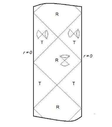
Figure 2: Carter-Penrose diagram for solution 2. Light cones are shown, indicating the temporal direction.

The scalar field $\phi$ in the whole range of $x$ is found as

$$\phi=\pm\frac{4}{3F_{0}b^{2}}\biggl{(}2x+\frac{9b}{2}\ln\Big{|}\frac{x-3b}{x+3b}\Big{|}\biggr{)}+\phi_{0}$$ (40)

and is singular both at $x=\pm\infty$ and at the horizons $x=\pm 3b$, while $X=A\phi^{\prime 2}$ is infinite at $x=\pm\infty$ and finite at the horizons. We thus have one more example of a horizon where the space-time is nonsingular but the scalar field is infinite.

6 Conclusion

We have made an attempt to study static, spherically symmetric configurations in the context of k-essence theories defined by a general function $F(X,\phi)$, where $X$ is the usual kinetic term of a scalar field. The k-essence theories have been employed in inflationary and dark energy models, but little has been done concerning local objects like stars and black holes. This work intended to partly fill this gap.

We have proved a no-go theorem for the case where the k-essence theory has only $X$-dependence, $F(X,\phi)=f(X)$, stating that no black hole solution with finite horizon area is possible unless the derivative of the function $f(X)$ diverges at the horizon. A special solution has been found illustrating this no-go theorem: fixing $f(X)=F_{0}X^{n}$ we have found for $n=1/3$ a non-asymptotically flat solution, with a single horizon at which $f_{X}$ diverges while $X$ and $f$ are finite. The resulting configuration may be characterized as a black hole with a Schwarzschild-like interior immersed in an asymptotically singular space-time.

Another solution has been obtained by choosing $n=1/2$ and introducing a cosmological constant. This solution is also non-asymptotically flat, but now there are two horizons with infinite surface area. In this case, the function $f(X)$ is regular at the horizons but the scalar field $\phi$ diverges there. Beyond the horizons the space-time changes its signature ($-2\mapsto+2$) still remaining Lorentzian, and the solution describes there a Kantowski-Sachs anisotropic universe with singularities that can be reached by test bodies in finite proper time. Between the two horizons there is a static region with a wormhole geometry.

Both solutions exemplify situations where a violent behavior of a scalar field at a horizon still leaves its SET finite and regular, which in turn leads to a regular space-time geometry. We can recall just one such example in the literature, a black hole with a massless conformal scalar field [15] and its electrically charged counterpart [13].

It is desirable to study the stability of such solutions, in particular, the static region of solution 2. The stability conditions are a very important aspect of any black hole or wormhole type solution, which remains an especially interesting problem in the cases where scalar fields and wormhole throats are present [16, 17].

Acknowledgments

We are grateful to Nail Khusnutdinov and Carlos Herdeiro for helpful discussions. We thank FAPES (Brazil) and CNPq (Brazil) for partial financial support. The work of KB was partly performed within the framework of the Center FRPP supported by MEPhI Academic Excellence Project (contract 02. 03.21.0005, 27.08.2013).

References

- [1] C. Armendariz-Picon, V. Mukhanov and P. J. Steinhardt, Phys. Rev. D 63, 103510 (2001).
- [2] C. Armendariz-Picon, T. Damour and V. Mukhanov, Phys. Lett. B 458, 209 (1999).
- [3] C. Armendariz-Picon, V. Mukhanov, and P. J. Steinhardt, Phys. Rev. Lett. 85, 4438 (2000).
- [4] R. Leigh, Mod. Phys. Lett. A4, 2767 (1989).
- [5] K. A. Bronnikov, G. Clément, C. P. Constantinidis, and J. C. Fabris, Grav. Cosmol. 4, 128 (1998).
- [6] K. A. Bronnikov, G. Clément, C. P. Constantinidis, and J. C. Fabris, Phys. Lett. A 243, 121 (1998).
- [7] K. A. Bronnikov, Phys. Rev. D 64, 064013 (2001); gr-qc/0104092.
- [8] K. A. Bronnikov and S. G. Rubin, Black Holes, Cosmology and Extra Dimensions (World Scientific, Singapore, 2012).
- [9] S. Adler and R. B. Pearson, Phys. Rev. D 18, 2798 (1978).
- [10] K. A. Bronnikov, S. B. Fadeev and A. V. Mishtchenko, Gen. Rel. Grav. 35, 505 (2003); gr-qc/0212065.
- [11] I. Z. Fisher, Zh. Eksp. Teor. Fiz. 18, 636 (1948); gr-qc/9911008.
- [12] H. Ellis, J. Math. Phys. 14, 104 (1973).
- [13] K. A. Bronnikov, Acta Phys. Pol. B4, 251 (1973).
- [14] V. Sahni and A. A. Sen, A new recipe for CDM, arXiv: 1510.09010.
- [15] N. M. Bocharova, K. A. Bronnikov, and V. N. Melnikov. Vestn. MGU, Fiz., Astron., No.6, 706 (1970).
- [16] J. A. Gonzalez, F. S. Guzman, and O. Sarbach, Class. Quantum Grav. 26,, 015010 (2009); Arxiv: 0806.0608.
- [17] K. A. Bronnikov, J. C. Fabris, and A. Zhidenko, Eur. Phys J. C 71, 1791 (2011).