Topological phases of lattice bosons with a dynamical gauge field

Abstract

Optical lattices with a complex-valued tunnelling term have become a standard way of studying gauge-field physics with cold atoms. If the complex phase of the tunnelling is made density-dependent, such system features even a self-interacting or dynamical magnetic field. In this paper we study the scenario of a few bosons in either a static or a dynamical gauge field by means of exact diagonalization. The topological structures are identified computing their Chern number. Upon decreasing the atom-atom contact interaction, the effect of the dynamical gauge field is enhanced, giving rise to a phase transition between two topologically non-trivial phases.

I Introduction

The external motion of a particle can be coupled to the dynamics of internal degrees of freedom via a gauge potential. The simplest example of this mechanism is that of an electrically charged particle moving in the presence of a background magnetic field. The gauge field imprints a complex $U(1)$ phase onto the wave function of the particle. The synthetic implementation of this mechanism in cold atomic systems has been envisaged since the early days of quantum gases Cooper and Wilkin (1999); Jaksch and Zoller (2003); Mueller (2004); Ruseckas et al. (2005); Osterloh et al. (2005); Cooper (2008); Dalibard et al. (2011), and has been realized successfully during the last years Lin et al. (2009a, b, 2011); Struck et al. (2012); Jiménez-García et al. (2012); Aidelsburger et al. (2011). Current quantum simulation with artificial gauge potentials are exploring the variety of interesting physics related to background gauge fields: spin liquid phases Struck et al. (2013), topological phases evidenced by non-zero Chern numbers Aidelsburger et al. (2015), or quantum Hall phases with edge currents Mancini et al. (2015); Stuhl et al. (2015). A long-term goal is the simulation of quantum electromagnetism or chromodynamics, that is, of models where matter interacts with dynamical fields, as described in Refs. Zohar et al. (2012); Tagliacozzo et al. (2013a); Banerjee et al. (2013); Zohar et al. (2013); Tagliacozzo et al. (2013b). An intermediate step might be the realization of simpler but nevertheless dynamical gauge fields, engineering an occupation number-dependent tunnelling term Edmonds et al. (2013); Greschner et al. (2014); Keilmann et al. (2011); Dutta et al. (2015); Greschner and Santos (2015); Greschner et al. (2015); Przysiȩżna et al. (2015); Bermudez and Porras (2015).

In this article, we consider a specific dynamical gauge field and apply exact diagonalization techniques to shed light on the involved interplay between the atoms’ external degree of freedom and the system’s $U(1)$ gauge potential. The atoms are confined to a two-dimensional optical lattice, where a gauge field is present due to a density-dependent complex phase of the tunnelling parameter $t$. Deep in the Mott phase, where density fluctuations are strongly suppressed, the gauge potential is static. We follow the system’s evolution upon decreasing the ratio $U/t$, where $U$ parametrizes the strength of the repulsive on-site interactions. For sufficiently weak interactions, topological transitions, not present in the system with a static gauge field, are found in the system with a dynamical gauge potential.

In our study the system is assumed to be close to filling one, where for large enough atom-atom interaction the Mott insulating state provides a vacuum-like configuration. In the strongly interacting regime, an extra-particle on top of the Mott insulator can be viewed as a single particle in a static gauge potential with a fixed magnetic flux per plaquette. This configuration therefore reproduces Hofstadter physics Hofstadter (1976). Due to computational limitations, our study addresses a 3$\times$3 lattice with $4\pi/3$ flux per plaquette. Twisted periodic boundary conditions allow for reducing finite-size effects. The low-energy subspace is clearly divided into three gapped bands. Chern number calculations demonstrate the non-trivial topological nature of the bands. Since a hole in the Mott insulator does not feel any gauge potential, the extra-particle configuration also captures the behavior in a larger Mott insulator with a particle-hole excitation. Upon decreasing the interaction, we find deviations from this single-particle picture. For a dynamical gauge potential we find that the ground state undergoes a topological phase transition before it becomes topologically trivial in the limit $U\rightarrow 0$.

The article is organized as follows. First, in Sec: II, we describe our theoretical tools, including the density dependent Hamiltonian we are considering. Then in Sec. III we present results for the different band gaps found, comparing the case of a dynamical field and the one of an static external field. The characterization of the topological properties by means of Chern numbers is presented in Sec. IV. In Sec. V a phase diagram trough a Mean Field approach is presented in order to give an intuitive idea of the behaviour of the system in the infinite size case. Finally, in Sec. VI we provide a brief summary and conclusions. In addition, the Appendix A includes the procedure used to compute Chern numbers for the many-body bands to characterize the topological phases.

II Theoretical model

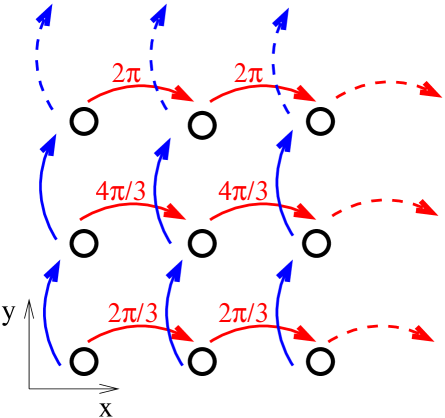
Figure 1: Brief rendition of the considered density dependent Hamiltonian. As an example we provide the phase acquired for the single particle case, $\hat{\cal H}_{\rm Landau}$, with $\varphi=2\pi/3$. The solid lines represent the tunnelling terms, the dashed ones correspond to the periodic boundary conditions considered.

Cold atoms in optical lattices are well described by a Hubbard model combining nearest-neighbour hopping processes and on-site interactions M. Lewenstein et al. (2012). The effect of a (synthetic) magnetic field is taken into account by a Peierls phase in the hopping parameter. For instance, if $\hat{b}_{k,l}$ ($\hat{b}_{k,l}^{\dagger}$) denotes the annihilation (creation) of a particle at site $(k,l)$, the hopping term in a constant magnetic field with magnetic flux $\varphi$ per plaquette is written in the Landau gauge as

$$\hat{\mathcal{H}}_{\rm Landau}=-t\sum_{k,l}\left({\rm e}^{{\rm i}\varphi l}\hat{b}^{\dagger}_{k,l}\hat{b}_{k+1,l}+\hat{b}^{\dagger}_{k,l}\hat{b}_{k,l+1}+{\rm h.c.}\right)\,.$$ (1)

Here, $t$ is a real-valued parameter associated with the kinetic energy of the particles. We consider a two-dimensional system of scalar bosons. Important quantities like the energy spectrum of the Hamiltonian are gauge-independent, that is, alternative hopping Hamiltonians with complex phases along the $x$-direction or along both the $x$- and $y$-direction would lead to the same results as long as the flux per plaquette remains the same. A schematic representation of the hopping structure is given in Fig. 1.

A possible implementation of Hamiltonians like $\hat{\mathcal{H}}_{\rm Landau}$ goes back to Ref. Jaksch and Zoller (2003). In this paper, we are interested in a situation where the gauge field becomes dynamical, that is, the complex phase factor should in some form depend on the positions of the atoms. A simple dynamical gauge field is obtained by letting the phase depend on the occupation numbers,

$$\hat{\mathcal{H}}_{\rm dyn}= -t\sum_{k,l}\Big{(}\hat{b}^{\dagger}_{k,l}{\rm e}^{{\rm i}\varphi l\left(\hat{n}_{k,l}+\hat{n}_{k+1,l}\right)}\hat{b}_{k+1,l}$$

$$+\hat{b}^{\dagger}_{k,l}\hat{b}_{k,l+1}+{\rm h.c.}\Big{)}\,.$$ (2)

The experimental implementation of density-dependent gauge fields as those of Hamiltonian (2) can be done using similar techniques as those recently discussed in Refs. Greschner and Santos (2015); Greschner et al. (2015). Particular details of how to implement it fall beyond the scope of the present article.

This choice of the density dependent field is particularly attractive as it has one specific limit in which the topological properties of the system can be easily understood. Deep in the Mott insulating phase, where the number operators $\hat{n}_{k,l}$ can be replaced by an integer number $n$, this Hamiltonian reduces to the form of a $\hat{\mathcal{H}}_{\rm Landau}$. The amount of particle number fluctuations and thereby the dynamical features of the gauge potential are controlled by the interaction term, $\hat{\mathcal{H}}_{\rm int}=\frac{U}{2}\sum_{k,l}\hat{n}_{k,l}(\hat{n}_{k,l}-1)$. With this, the full Hamiltonian reads

$$\hat{\mathcal{H}}=\hat{\mathcal{H}}_{\rm dyn}+\hat{\mathcal{H}}_{\rm int}\,.$$ (3)

We will take an additional constraint on the Hilbert space, stemming from the implementation scheme described in Ref. Greschner and Santos (2015), namely, the maximum occupancy per site will be set to two bosons.

To clarify our discussion we will compare our results to those obtained with an static field, that is,

$$\hat{\mathcal{H}}_{\rm st}=\hat{\mathcal{H}}_{\rm Landau}+\hat{\mathcal{H}}_{\rm int}\,.$$ (4)

III Energy gaps

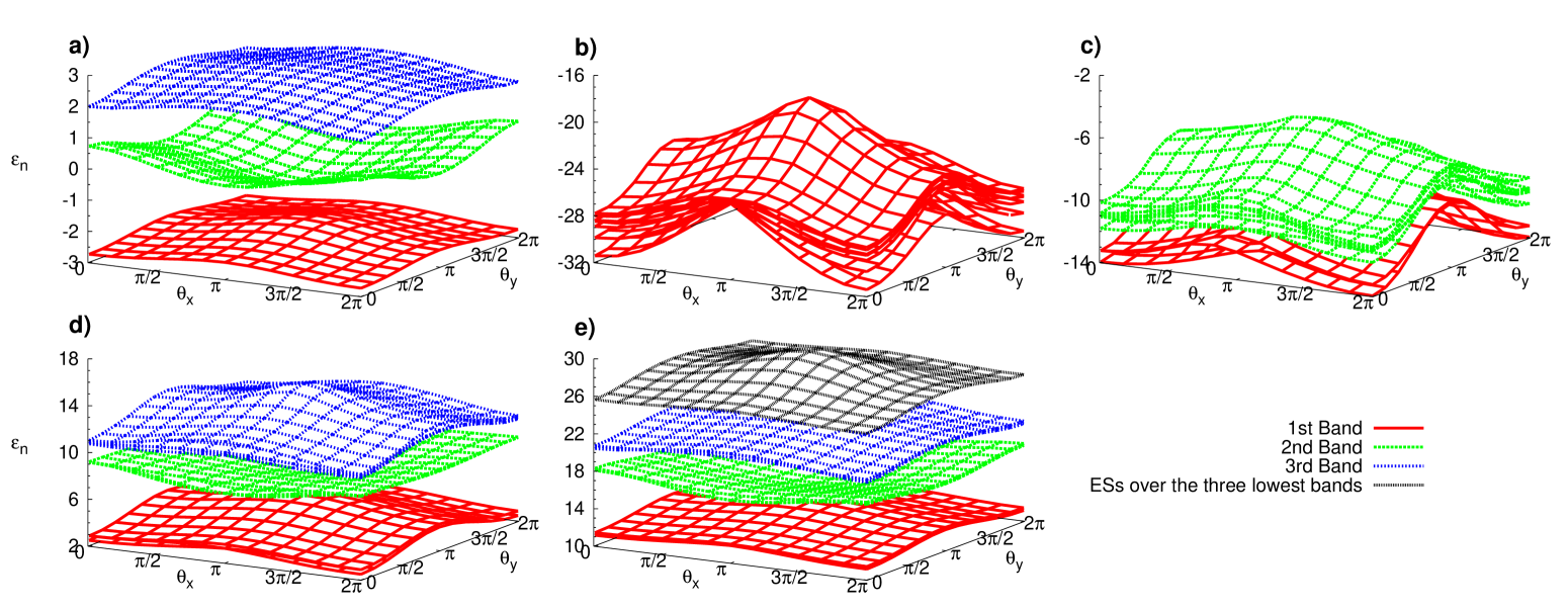
Figure 2: Energy spectrum as a function of the twisted boundary conditions for several systems under $\hat{\cal H}_{\rm st}$ with a flux per plaquette $\varphi=2\pi/3$ in a $3\times 3$ lattice. Degenerated states forming bands have the same color. a) Single particle case. b)–e) Energies of the ten lowest eigenstates of the system with 10 particles for the interaction values: b) $U=0t$, c) $U=4t$, d) $U=13t$ and e) $U=20t$. ESs means Excited States.

We have concentrated on the filling case around one by means of exact diagonalization. We have focused on a 3$\times$3 lattice at $\varphi=4\pi/3$, and take the interaction strength $U$ (in units of $t$) as the main tuning parameter. As argued above, this also controls the influence of the dynamical gauge field. To gain meaningful results despite the small system size, we apply twisted boundary conditions with twist angles $\theta_{x}$ and $\theta_{y}$. With this, the energy spectrum $\epsilon_{i}$ of the Hamiltonian becomes a function of the twist angles, $\epsilon_{i}(\theta_{x},\theta_{y})$. Degeneracies of different levels which would be lifted due to the finite system size manifest themselves in crossings of bands $\epsilon_{i}(\theta_{x},\theta_{y})$. Accordingly, we define the gap above a level $\epsilon_{i}$ as

$$\Delta\epsilon_{i}={\rm min}\left[\epsilon_{i+1}\left(\theta_{x},\theta_{y}\right)-\epsilon_{i}\left(\theta_{x},\theta_{y}\right)\right]\,.$$ (5)

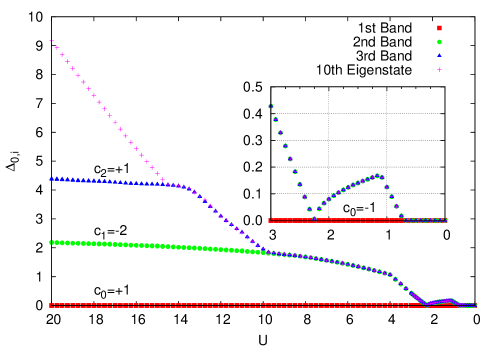
Figure 3: Gap above each band, [as defined in Eq. (6)], between consecutive eigenstates of $\hat{\mathcal{H}}$ as function of the on-site interaction parameter $U$. The system is a $3\times 3$ lattice with $10$ particles with the parameter $\varphi=2\pi/3$ and $t=1$. We take into account the Hilbert constraint to a maximum of two bosons per site. The three lowest bands have degeneracy 3. and the labels correspond to the Chern number of each band.

If $\Delta\epsilon_{i}$ is zero, that is, if band $i$ and band $i+1$ have (at least) one crossing, we consider these levels a degenerate manifold. To check whether the manifold is separated from higher levels by a gap, we then have to consider $\Delta\epsilon_{i+1}$. In general, the gap above a $k$-fold manifold including the levels $i,\dots,i+k$ is defined as

$$\Delta_{i,i+k}=\sum_{j=i}^{i+k-1}\Delta\epsilon_{j}\,.$$ (6)

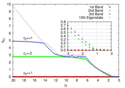
Figure 4: Same description as in Fig. 3, but with the dynamical gauge field replaced by an external magnetic field with a flux per plaquette $\varphi=4\pi/3$. That is, $\hat{\cal{H}}\left(\phi\right)\rightarrow\hat{\cal{H}}_{\rm st}\left(2\phi\right)$.

III.1 Case of one excess particle

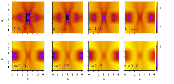
Figure 5: Energy difference between the third and fourth states in the spectrum of a system under $\hat{\cal H}$ with 10 particles in a $3\times 3$ lattice, signaling the gap between the ground state manifold and next excited state. The different panels correspond to different values of $U$. In all cases, $\varphi=2\pi/3$ and $t=1$.

We start our analysis with the tunnelling of a system with one particle more than the number of sites. That is, in our $3\times 3$ lattice we consider $N=10$ bosons. On the strongly interacting side, this is equivalent to having a single particle on top of a fluctuating vacuum. For large $U$, fluctuations are strongly suppressed, and the kinetic Hamiltonian (II) reduces to the one of a particle in a static magnetic field, Eq. (1), with flux 2$\varphi$. Accordingly, the physics of a single particle in a magnetic field should describe the low-energy behavior of our system. Indeed, no difference is seen between the shape of the single-particle spectrum of the Hamiltonian (1), Fig. 2 a), and the (low-energy part) of the one of the many-body spectrum of Hamiltonian (3) at large $U$, Fig. 2 e). In both cases, we find the energy spectrum to be split into three gapped manifolds, each of them consisting of three states. In the many-body system, a gapless high-energy manifold lies above the third band.

Deviations from this structure appear when $U$ is decreased, see Fig. 2(b–e) and Fig. 3. The dynamical mechanism is the following. As $U$ is decreased, the number of holon-doublon excitations increases, the single-particle picture described above is no-longer valid. First, for $U\approx 15$, the gap between the third band and the high-energy manifold closes, as the first doublon-holon excitations have the same energy as the third single particle state. Subsequently, at $U\approx 10$, also the gap to the second band is closed. These gap closings indicate phase transitions in excited states. At $U\simeq 2.25$, also the gap to the lowest band is closed. Thus, up to $U\simeq 2.25$ the ground state manifold has a topological structure similar to the case of a single particle subjected to an external magnetic field of $2\varphi$. This value of $U$ is a bit higher than the value at which we found a gappless phase for the filling one case described below. Thus, the main picture of a single particle on top of a Mott insulating background is consistent.

Remarkably, further lowering the value of the interaction another threefold-degenerate gapped manifold appears for $0.67\lesssim U\lesssim 2.25$. Only for $U\lesssim 0.67$ the system enters in a gapless phase. We note that for $0.67\lesssim U\lesssim 2.25$ the gap is small, of the order of 10% of the involved energy scales. It is a merit of the twisted boundary conditions that the three lowest states are clearly identified as an adiabatically connected manifold, separated from the other levels by a gap. In fact, if we look at the system for a fixed value of $\theta_{x}$ and $\theta_{y}$, or alternatively for open boundary conditions, the gap cannot be distinguished from the energy splitting between states in the degenerate manifold. The evolution of the gap between the ground state manifold and the next excited state for the all values of $\theta_{x}$ and $\theta_{y}$ is given in Fig. 5. The gap above a manifold as function of $U$ is shown in Fig. 3 . For $U\simeq 0.67$ the gap closes at $(\theta_{x},\theta_{y})\simeq(\pi,\pi)$. The next closing, for $U\simeq 2.25$ appears close to $(\theta_{x},\theta_{y})\simeq(0,\pi)$. This could diminish the prospects for an experimental detection of this phase in the plane geometry, but since an experiment would realize a much bigger system, there is hope that finite-size degeneracy splitting would be sufficiently small to identify the finite gap.

In Fig. 4, we contrast our findings to the scenario with static magnetic field. As expected, at large $U$ the differences between Fig. 3 and 4 are minor. Also for a static magnetic field, increasing $U$ subsequently closes the gaps above the third and the second band. However, the gap above the ground state remains finite up to $U\simeq 1$ and, for $U<1$, it vanishes.

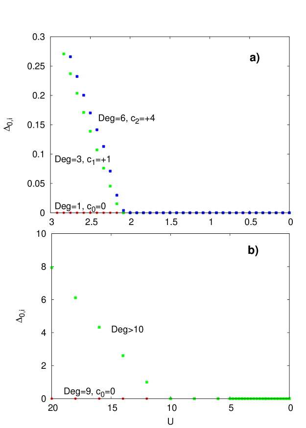
Figure 6: Energy gap, see Eq. (6), between consecutive eigenstates of $\hat{\mathcal{H}}$ as function of the on-site interaction parameter $U$. We take into account the Hilbert constraint to a maximum of two bosons per site. The upper and lower panels are for $N=9$ and $N=8$, respectively.

III.2 Mott insulator

At precisely filling one, for 9 particles on 9 lattice sites, see the upper panel of Fig. 6, we find a unique gapped ground state for $U\gtrsim 2.1$, which is connected to the Mott insulator as an exact solution for $U\rightarrow\infty$. This phase is trivial in the sense that it corresponds to a vacuum, where deviations from integer filling exist only as fluctuations. For $U\lesssim 2.1$, we find a gapless phase, that is, despite the presence of the dynamical gauge field, no topological structure protected by an energy gap emerges in this scenario.

The first and second excited bands are three- and six-fold degenerate, respectively. They are topologically non-trivial and their Chern numbers are $+1$ and $+4$. This excited bands coincide, in degeneracy and topology, with the lowest band of the non-interacting systems with one and two particles in the same lattice, as they are explained in Section IV. A. These excited bands can be understood as one and two particle-hole excitations on the top of the Mott insulator, when the particle feels an effective static magnetic field and the hole do not.

III.3 Case of one hole

We also study the tunnelling of a single hole. That is, in our $3\times 3$ lattice we consider $N=8$ bosons. The gap structure we find is shown in Fig. 6 b). As expected, we find that increasing the interaction up to $U\simeq 10t$, a gap opens between the nine-fold degenerate manifold, understood as one hole moving in the Mott-insulating background, and the rest of the states. The ground state manifold is found to have a trivial topological order.

IV Topological phases

In the previous section we have discussed the energy gaps appearing for the case of one excess particle, the filling one, and the one hole case. The only case in which we have found non-trivial topological structures is for the case of one excess particle. In the following we present the Chern number obtained compared to the case of an external field of flux $4\pi/3$.

IV.1 Single particle and non-interacting cases

First, we calculate the Chern numbers of the single-particle system described by $\hat{\mathcal{H}}_{\rm Landau}$, that is, of the bands shown in Fig. 2 a). We obtain the values $\{1,-2,1\}$. In this case, the calculation can either be done via Fourier transformation, taking the parameters $k_{1}$ and $k_{2}$ to be components of the wave vector Thouless et al. (1982), or with twisted boundary conditions, taking the twist angles $\theta_{x}$ and $\theta_{y}$ as parameters $k_{1}$ and $k_{2}$ Niu et al. (1985). In the latter case, the discretization of parameter space is arbitrary, but we observe quick convergence of the Chern numbers to fixed numbers upon refining the discretization.

The non-interacting case can be related to the single particle case although some caution should be exercised. For instance, direct computation of the Chern number of the ground state manifold for $N=2$, $3$, and $4$ particles in the $3\times 3$ lattice we consider gives $c=4,10$ and $20$, respectively. These can be obtained by noting that due to the bosonic symmetry, we have a combinatorial factor stemming from the number of times the Fock basis covers the threefold degenerate band. This can be evaluated giving,

$$c_{0}^{\left(N\right)}=\frac{N}{3}\binom{N+3-1}{N}c_{0}^{\left(1\right)}=c_{0}^{\left(1\right)}\,\binom{N+2}{3}\,,$$ (7)

where $c_{0}^{\left(1\right)}$ is the single particle Chern number of the GS manifold, $c_{0}^{\left(1\right)}=1$.

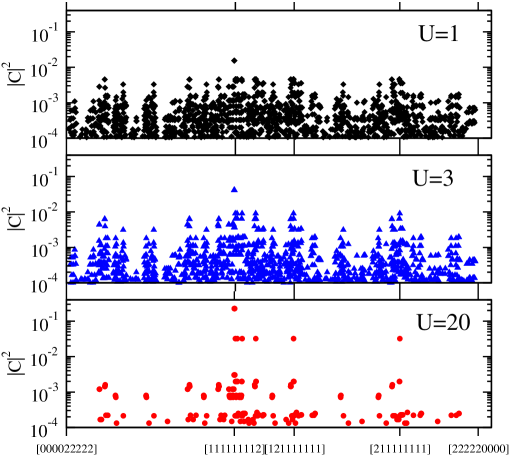
Figure 7: Squared coefficients of the ground state of the density dependent ${\cal\hat{H}}$ for $\theta_{x}=\theta_{y}=0$ in the Fock basis in lexicographical order. A few notable states, one particle on top of a Mott insulator, are marked. The three panels corresponds to three values of the interaction, $U=1,3$ and $20$. For these values, the Chern number of the ground state manifold is $-1$, $+1$ and, $+1$, respectively.

IV.2 Interacting many-body case

To calculate the Chern numbers of many-body states, we exclusively resort to the twisted boundary conditions. For the three gapped manifolds appearing at $U\lesssim 15$, see Fig. 3, we obtain the same Chern numbers as for the single particle bands: $\{1,-2,1\}$. These numbers remain constant for each manifold until the closing of the corresponding gap. Upon closing the gap, the second and the third bands simply merge with the energy continuum, for which no Chern number can be computed. This is easily understood as for large enough interactions the many-body ground state is well described as consisting on a Mott-insulating background plus one particle. The lower band is given by the energy of the extra particle in the presence of an external field with flux $4\pi/3$. The closing of the bands in the higher part of the spectrum comes from the first particle-hole excitations which eventually degenerate with excitations of the excess particle. Note that even though this simple picture provides a compelling explanation it is quite remarkable that albeit the many-body state changes, as shown in Fig. 7, as $U$ is decreased, the topology of the band does not change for a broad range of $U$.

In contrast with the above, the gap closing of the ground state at $U\approx 2.25$ separates two gapped regions, see in particular the inset of Fig. 3. Interestingly, we find that upon closing the band gap, the ground state Chern number changes its sign from $1$ to $-1$. This demonstrates that a topological phase transition between two distinct, but topologically non-trivial phases is taking place. The second gap closing, at $U\approx 0.67$, merges the ground state manifold with the energy continuum which, in this sense, is a transition to a topologically trivial (gapless) phase.

IV.3 Static field case

Finally, we note also that the three gapped manifolds found for a system with static magnetic field, with $\phi=4\pi/3$, are characterized by the same Chern numbers $\{1,-2,1\}$, without any transitions to distinct gapped phases. As seen in Fig. 4, the arguments exposed above also apply to this case and the picture of a single particle on top of a Mott-insulator is perfectly valid. The only relevant difference appears for low interaction energies. In this case, the Mott insulating phase seems to survive down to lower values of the interaction as compared to the density dependent case. Thus, density dependence phases favor the existence of superfluid regimes at larger interactions than in the static case. Also we find no trace of the first excitation being a topological phase with $c_{1}=+1$ in the region $2.25\gtrsim U\gtrsim 0.67$. In this case the limit $U=0$ can be understood from the single-particle calculation: The ground states for $N$ bosons are just arbitrary distributions on the $M=N_{\rm s}/q$ states belonging to the lowest energy band in a lattice with $N_{\rm s}$ sites at magnetic flux $2\pi/q$. This leads to a macroscopic ground state degeneracy (of 63 states in our case with $N=10$, $N_{\rm s}=9$, and $q=3$), for which no meaningful Chern number can be defined. Recent “Chern number” measurements in non-interacting bosonic quantum gases Aidelsburger et al. (2015) consider the Hall drift for unique but gapless many-body states, and define as a “Chern number” the average over different states.

V Mean field Phase diagram

In order to get a picture of the phase diagram, we have adapted the Mean-field calculation of Ref. Keilmann et al. (2011) to the Hamiltonians of interest. At first, we include a chemical potential term $-\mu\sum_{i,j}\hat{n}_{i,j}$. With the convenient substitutions $\hat{c}_{i,j}\equiv e^{{\rm i}\phi j\hat{n}_{i,j}}\hat{b}_{i,j}$ and $\hat{d}_{i,j}\equiv e^{-{\rm i}\phi j\hat{n}_{i,j}}\hat{b}_{i,j}$, the Hamiltonian in Eq. (3) looks like,

$$\hat{\mathcal{H}}= \sum_{k,l}\Big{\{}-t\Big{(}\hat{d}^{\dagger}_{k,l}\hat{c}_{k+1,l}+\hat{b}^{\dagger}_{k,l}\hat{b}_{k,l+1}+{\rm h.c.}\Big{)}$$

$$+\hat{n}_{k,l}\left[\left(\hat{n}_{k,l}-1\right)\frac{U}{2}-\mu\right]\Big{\}}\,.$$ (8)

At $t=0$, all the sites are independent and the GS can exactly be represented with a Gutzwiller ansatz,

$$|\Psi_{0}\rangle=\bigotimes_{k,l}^{N_{\rm s}}|\psi\rangle_{k,l},\qquad|\psi\rangle_{k,l}=\sum_{m=0}^{\infty}f_{k,l}^{\left(m\right)}|m\rangle_{k,l},$$ (9)

where $m$ is the number of particles in a site. Then, the energy due to each site filled with $m$ particles is $\epsilon_{m}=U\left[\frac{1}{2}\left(m-1\right)-\frac{\mu}{U}\right]m$. and the energy of adding and subtracting one boson is,

$$\epsilon_{m+1}-\epsilon_{m}=U\left(m-\frac{\mu}{U}\right),\qquad\epsilon_{m-1}-\epsilon_{m}=U\left(\frac{\mu}{U}-m+1\right),$$ (10)

respectively.

The MF is obtained by decoupling the hopping terms as $\hat{d}_{i,j}^{\dagger}\hat{c}_{i+1,j}\approx\alpha_{3,j}^{*}\hat{c}_{i+1,j}+\alpha_{2,j}\hat{d}_{i,j}^{\dagger}-\alpha_{3,j}^{*}\alpha_{2,j}$ and $\hat{b}_{i,j}^{\dagger}\hat{b}_{i,j+1}\approx\alpha_{1,j}^{*}\hat{b}_{i,j+1}+\alpha_{1,j+1}\hat{b}_{i,j}^{\dagger}-\alpha_{1,j}^{*}\alpha_{1,j+1}$, with the order parameters $\alpha_{1,j}\equiv\langle\hat{b}_{i,j}\rangle$, $\alpha_{2,j}\equiv\langle\hat{c}_{i,j}\rangle$ and, $\alpha_{3,j}\equiv\langle\hat{d}_{i,j}\rangle$. Then, the Hamiltonian in Eq. (V) becomes,

$$\hat{\mathcal{H}}= -N_{\rm x}t\sum_{j}\left(\alpha_{3,j}^{*}\alpha_{2,j}+\alpha_{1,j}^{*}\alpha_{1,j+1}+{\rm h.c.}\right)+\sum_{k,j}\hat{h}_{k,j},$$ (11)

with the local Hamiltonian

$$\hat{h}_{k,j}\equiv\hat{n}_{k,j}\left[U\left(\hat{n}_{k,j}-1\right)/2-\mu\right]-t\hat{T}_{k,j},$$ (12)

where $\hat{T}_{k,j}\equiv\alpha_{3,j}^{*}\hat{c}_{k,j}+\alpha_{2,j}\hat{d}^{\dagger}_{k,j}+\alpha_{1,j-1}^{*}\hat{b}_{k,j}+\alpha_{1,j+1}\hat{b}^{\dagger}_{k,j}+{\rm h.c.}$ and $N_{\rm x}$ is the size of the system in the $x$-direction. The Hamiltonian $\hat{h}_{k,j}$ has a trivial solution when $\alpha_{\gamma,j}=0$, $\gamma=1,2,3$ since the particle number fluctuations vanish at the Mott insulating phase.

When the kinetic term is negligible ($t\ll U$), the entire system is described with the basis of states with $m$ particles per each site $\left(k,j\right)$, $|m\rangle$. The GS is determined by $\mu$: it is the local state $|m\rangle$ when $m-1<\mu<m$. Since we want to draw the Mott lobes, we include the single Fock state and particle-hole excitations in that region of the diagram. Then, since we search the boundaries close to the trivial solution, $\left|\alpha_{\gamma,j}\right|\ll 1$, and the kinetic term can be treated perturbatively. Up to first perturbation order, the local wavefunction $|\Psi\rangle$ can be written as $|\psi^{\left(0\right)}\rangle+|\psi^{\left(1\right)}\rangle$, being $|\psi^{\left(0\right)}\rangle=|m\rangle$ and

$$|\psi^{\left(1\right)}\rangle= -t\sum_{m^{\prime}}\frac{\langle m^{\prime}|\hat{T}_{k,j}|m\rangle}{\epsilon_{m^{\prime}}-\epsilon_{m}}|m^{\prime}\rangle$$

$$= \frac{t}{U}\frac{\sqrt{m}\left[\alpha_{3,j}^{*}e^{{\rm i}\phi j\left(m-1\right)}+\alpha_{2,j}^{*}e^{-{\rm i}\phi j\left(m-1\right)}+\alpha_{1,j-1}^{*}+\alpha_{1,j+1}^{*}\right]}{\frac{\mu}{U}-\left(m-1\right)}|m-1\rangle$$

$$+\frac{t}{U}\frac{\sqrt{m+1}\left[\alpha_{3,j}e^{-{\rm i}\phi jm}+\alpha_{2,j}e^{{\rm i}\phi jm}+\alpha_{1,j-1}+\alpha_{1,j+1}\right]}{m-\frac{\mu}{U}}|m+1\rangle$$ (13)

The first order perturbation about the solution $\alpha_{\gamma,j}=0$ is convenient here, since the self-consistency equations define a linear map $\alpha_{\gamma,j}=\Lambda_{\gamma,j}^{\gamma^{\prime},j^{\prime}}\alpha_{\gamma^{\prime},j^{\prime}}$. Then, when the largest eigenvalue of $\Lambda$, $\lambda_{0}$, is larger than $1$, the trivial solution is no longer stable. So, the boundary is found to be at $\lambda_{0}=1$. The self-consistency relations $\alpha_{1,j}=\langle\Psi|\hat{b}_{k,j}|\Psi\rangle$, $\alpha_{2,j}=\langle\Psi|\hat{c}_{k,j}|\Psi\rangle$ and, $\alpha_{3,j}=\langle\Psi|\hat{d}_{k,j}|\Psi\rangle$ give,

$$\alpha_{1,j}=\frac{t}{U}\left[A\left(\alpha_{1,j-1}+\alpha_{1,j+1}\right)+f_{j}\left(\phi\right)\alpha_{2,j}+f_{j}\left(-\phi\right)\alpha_{3,j}\right]$$

$$\alpha_{2,j}=\frac{t}{U}\left[f_{j}\left(\phi\right)\left(\alpha_{1,j-1}+\alpha_{1,j+1}\right)+f_{j}\left(2\phi\right)\alpha_{2,j}+A\alpha_{3,j}\right]$$

$$\alpha_{3,j}=\frac{t}{U}\left[f_{j}\left(-\phi\right)\left(\alpha_{1,j-1}+\alpha_{1,j+1}\right)+A\alpha_{2,j}+f_{j}\left(-2\phi\right)\alpha_{3,j}\right]$$ (14)

with

$$f_{j}\left(\phi\right)\equiv\left[A+B\left(e^{-{\rm i}\phi j}-1\right)\right]e^{-{\rm i}\phi jm}$$

$$A\equiv\frac{\frac{\mu}{U}+1}{\left[\frac{\mu}{U}-\left(m-1\right)\right]\left[m-\frac{\mu}{U}\right]},\qquad B\equiv\frac{m}{\frac{\mu}{U}-\left(m-1\right)}.$$

For the case of the static magnetic field, the corresponding function $f_{j}^{\rm st}\left(\phi\right)$ reduces to $Ae^{-{\rm i}\phi j}$.

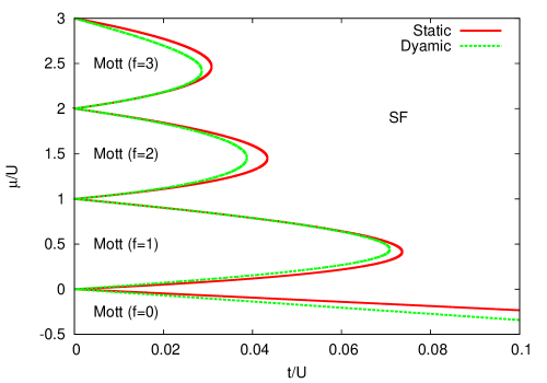
Figure 8: Phase boundary between the Mott insulator phase and the superfluid phase for the external and dynamical magnetic fields according to the Gutzwiller ansatz with the MF approach in the 1st perturbation order in the hopping $t$.

The Fock space populations of the GS of the system, Fig. 7, have revealed its structure: the Fock states which have a particle on top of a MI in the same row are equally populated. Then, we have tried an ansatz which is translationally invariant along the $x$-direction and have a 3-unit cell in the $y$-direction. So, in Eq. (14), $j=1,2,3$, without periodic boundary conditions. Then, those relations define a linear system of nine coupled linear equations, being $\alpha_{\gamma,j}$ the variables. Once the matrix of the system is diagonalized as function of $t$, for a numeric value of $U$, $\mu$ (and its corresponding integer $m$), the expression of $\lambda_{0}$ is set to $1$ and then the equation is solved for $t$. Finally, the phase boundary is obtained as a collection of points $\left(\mu,t\right)$.

We find the Mott lobes, shaped as usual in the MF approach, see Fig. 8. The values of the boundary do not correspond to the ones of the MF for the 2D lattice, but they are closer to the ones of the 1D case, see Ref. dos Santos and Pelster (2009). The structure of the GS state has revealed this to be closely related to the fact that the magnetic fields are in the Landau gauge. Our analysis also shows that the trial state is slightly more robust upon decreasing hopping $t/U$ in the dynamic field case than in the static one. This finding qualitatively agrees with our results for the gap separation in the exact diagonalization analysis: As seen in Figs. 3 and  4, the SF regime corresponds to the gapless phase at small $U$, which extends to $U=0.8$ in the dynamic case, and $U=1.2$ in the static case. For $\mu<0$, the boundaries of the dynamic field case and the 2D non-magnetic case coincide, as expected.

VI Summary and conclusions

We have studied topological properties of a bosonic quantum gas with an experimentally feasible, synthetic dynamical gauge field. The Mott insulating phase provides a trivial vacuum, above which we study the one-particle excitations, forming gapped energy bands. Decreasing the interactions, we first observe transitions in the excited bands, from topologically non-trivial phases to gapless phases. In this respect, the system behavior does not differ from the one of a system with static magnetic field. A particular feature of the dynamic gauge field is a topological transition in the ground state, in which the sign of the Chern number is inverted. The fact that in our proposal the length of the system in one dimension is very small could be accomplished in a experimental set-up using synthetic dimensions.

Acknowledgements. We thank S. Greschner, T. Mishra, and M. Rizzi for discussions. Financial support from EU grants EQuaM (FP7/2007-2013 Grant No. 323714), OSYRIS (ERC-2013-AdG Grant No. 339106), QUIC (H2020-FETPROACT-2014 No. 641122) and, SIQS (FP7-ICT-2011-9 No. 600645), MINECO grant FOQUS (FIS2013-46768-P) and “Severo Ochoa” Programme (SEV-2015-0522), Generalitat de Catalunya grants 2014 SGR 401 and 2014 SGR 874 and, Fundació Cellex is acknowledged. B.J-D. is supported by the Ramon y Cajal program. L.S. thanks the Center for Quantum Engineering and Space-Time Research, and the DFG Research Training Group 1729.

Appendix A Evaluation of the Chern number

The twisted boundary conditions are particularly useful to characterize topological phases. They allow one to define Chern numbers in an interacting many-body system Niu et al. (1985). Quite generally, the Chern number is defined for the energy levels $n$ of a Hamiltonian ${\cal H}(k_{1},k_{2})={\cal H}(k_{1}+2\pi,k_{2})={\cal H}(k_{1},k_{2}+2\pi)$, which periodically depends on two parameters $k_{1}$ and $k_{2}$ in the following way,

$$c_{n}=\frac{1}{2\pi{\rm i}}\int_{0}^{2\pi}dk_{1}\int_{0}^{2\pi}dk_{2}\;F_{12}^{\left(n\right)}\left(k_{1},k_{2}\right)$$ (15)

where the Berry connection ${\cal A}_{\mu}^{\left(n\right)}(k_{1},k_{2})$ ($\mu=1,2$) and the associated strength $F_{12}^{\left(n\right)}(k_{1},k_{2})$ are given by

$${\cal A}_{\mu}^{\left(n\right)}(k_{1},k_{2})=\left<n(k_{1},k_{2})\right|\partial_{\mu}\left|n(k_{1},k_{2})\right>$$ (16)

$$F_{12}^{\left(n\right)}(k_{1},k_{2})=\partial_{1}{\cal A}_{2}^{(n)}(k_{1},k_{2})-\partial_{2}{\cal A}_{1}^{\left(n\right)}(k_{1},k_{2})$$ (17)

with $\left|n\left(k_{1},k_{2}\right)\right>$ being the $n$th normalized eigenvector.

Following the method of Fukui et al. Fukui et al. (2005), the Chern numbers can conveniently be calculated by discretizing the parameter space,

$$\tilde{c}_{n}=\frac{1}{2\pi{\rm i}}\sum_{k_{1}}\sum_{k_{2}}\tilde{F}_{12}^{\left(n\right)}\left(k_{1},k_{2}\right)$$ (18)

with the lattice field strength,

$$\begin{split}&\tilde{F}_{12}^{\left(n\right)}\left(k_{1},k_{2}\right)=\ln{\left[\frac{U_{1}^{\left(n\right)}(k_{1},k_{2})\,U_{2}^{\left(n\right)}(k_{1}+dk_{1},k_{2})}{U_{1}^{\left(n\right)}(k_{1},k_{2}+dk_{2})\,U_{2}^{\left(n\right)}(k_{1},k_{2})}\right]},\\ &-\pi<\frac{1}{\rm i}\tilde{F}_{12}^{\left(n\right)}\left(k_{1},k_{2}\right)\leq\pi\end{split}$$ (19)

being $dk_{\mu}$ the resolution of each parameter and $U_{\mu}^{\left(n\right)}$ the link variables from the eigenstates of the $n$th band,

$$U_{\mu}^{\left(n\right)}\equiv\frac{\left<n(k_{1},k_{2})\big{|}n(k_{1}+dk_{1}\delta_{1,\mu},k_{2}+dk_{2}\delta_{2,\mu})\right>}{\left|\left<n(k_{1},k_{2})\big{|}n(k_{1}+dk_{1}\delta_{1,\mu},k_{2}+dk_{2}\delta_{2,\mu})\right>\right|}\,.$$ (20)

A special case which is important for our purposes concerns the Chern number of degenerate bands. Since the eigenstates are not unique in the degenerate points, we cannot associate Chern numbers to individual states. For $M$ degenerate or quasi-degenerate states, we consider the multiplet $\psi=\left(\left|n_{1}\right>\cdots\left|n_{M}\right>\right)$ to define a non-Abelian Berry connection ${\cal A}=\psi^{\dagger}d\psi$, which is an $M\times M$ matrix-valued one form associated to $\psi$. Then, we consider the overlap matrix

$$\left[u_{\mu}^{\left(n\right)}\right]_{ij}\equiv\left<n_{i}(k_{1},k_{2})\big{|}n_{j}(k_{1}+dk_{1}\delta_{1,\mu},k_{2}+dk_{2}\delta_{2,\mu})\right>,$$ (21)

in order to properly define the link variables

$$U_{\mu}^{\left(n\right)}\equiv\frac{\det{\left[u_{\mu}^{\left(n\right)}\right]}}{\left|\det{\left[u_{\mu}^{\left(n\right)}\right]}\right|}$$ (22)

Finally, the Chern number $\tilde{c}_{\psi}$ and field strength are calculated using Eqs. (18) and (LABEL:F).

References

- Cooper and Wilkin (1999) N. R. Cooper and N. K. Wilkin, Phys. Rev. B 60, R16279 (1999).
- Jaksch and Zoller (2003) D. Jaksch and P. Zoller, New J. Phys. 5, 56 (2003).
- Mueller (2004) E. J. Mueller, Phys. Rev. A 70, 041603 (2004).
- Ruseckas et al. (2005) J. Ruseckas, G. Juzeliūnas, P. Öhberg, and M. Fleischhauer, Phys. Rev. Lett. 95, 010404 (2005).
- Osterloh et al. (2005) K. Osterloh, M. Baig, L. Santos, P. Zoller, and M. Lewenstein, Phys. Rev. Lett. 95, 010403 (2005).
- Cooper (2008) N. Cooper, Adv. Phys. 57, 539 (2008).
- Dalibard et al. (2011) J. Dalibard, F. Gerbier, G. Juzeliūnas, and P. Öhberg, Rev. Mod. Phys. 83, 1523 (2011).
- Lin et al. (2009a) Y.-J. Lin, R. L. Compton, K. Jiménez-García, J. V. Porto, and I. B. Spielman, Nature 462, 628 (2009a).
- Lin et al. (2009b) Y.-J. Lin, R. L. Compton, A. R. Perry, W. D. Phillips, J. V. Porto, and I. B. Spielman, Phys. Rev. Lett. 102, 130401 (2009b).
- Lin et al. (2011) Y. J. Lin, K. Jiménez-García, and I. B. Spielman, Nature 471, 83 (2011).
- Struck et al. (2012) J. Struck, C. Ölschläger, M. Weinberg, P. Hauke, J. Simonet, A. Eckardt, M. Lewenstein, K. Sengstock, and P. Windpassinger, Phys. Rev. Lett. 108, 225304 (2012).
- Jiménez-García et al. (2012) K. Jiménez-García, L. J. LeBlanc, R. A. Williams, M. C. Beeler, A. R. Perry, and I. B. Spielman, Phys. Rev. Lett. 108, 225303 (2012).
- Aidelsburger et al. (2011) M. Aidelsburger, M. Atala, S. Nascimbène, S. Trotzky, Y.-A. Chen, and I. Bloch, Phys. Rev. Lett. 107, 255301 (2011).
- Struck et al. (2013) J. Struck, M. Weinberg, C. Olschlager, P. Windpassinger, J. Simonet, K. Sengstock, R. Hoppner, P. Hauke, A. Eckardt, M. Lewenstein, and L. Mathey, Nat. Phys. 9, 738 (2013).
- Aidelsburger et al. (2015) M. Aidelsburger, M. Lohse, C. Schweizer, M. Atala, J. T. Barreiro, S. Nascimbene, N. R. Cooper, I. Bloch, and N. Goldman, Nat. Phys. 11, 162 (2015).
- Mancini et al. (2015) M. Mancini, G. Pagano, G. Cappellini, L. Livi, M. Rider, J. Catani, C. Sias, P. Zoller, M. Inguscio, M. Dalmonte, and L. Fallani, Science 349, 1510 (2015).
- Stuhl et al. (2015) B. K. Stuhl, H.-I. Lu, L. M. Aycock, D. Genkina, and I. B. Spielman, Science 349, 1514 (2015).
- Zohar et al. (2012) E. Zohar, J. I. Cirac, and B. Reznik, Phys. Rev. Lett. 109, 125302 (2012).
- Tagliacozzo et al. (2013a) L. Tagliacozzo, A. Celi, A. Zamora, and M. Lewenstein, Ann. Phys. 330, 160 (2013a).
- Banerjee et al. (2013) D. Banerjee, M. Bögli, M. Dalmonte, E. Rico, P. Stebler, U.-J. Wiese, and P. Zoller, Phys. Rev. Lett. 110, 125303 (2013).
- Zohar et al. (2013) E. Zohar, J. I. Cirac, and B. Reznik, Phys. Rev. Lett. 110, 125304 (2013).
- Tagliacozzo et al. (2013b) L. Tagliacozzo, A. Celi, P. Orland, M. W. Mitchell, and M. Lewenstein, Nat. Commun. 4, 2615 (2013b).
- Edmonds et al. (2013) M. J. Edmonds, M. Valiente, G. Juzeliūnas, L. Santos, and P. Öhberg, Phys. Rev. Lett. 110, 085301 (2013).
- Greschner et al. (2014) S. Greschner, G. Sun, D. Poletti, and L. Santos, Phys. Rev. Lett. 113, 215303 (2014).
- Keilmann et al. (2011) T. Keilmann, S. Lanzmich, I. McCulloch, and M. Roncaglia, Nat. Commun. 2, 361 (2011).
- Dutta et al. (2015) O. Dutta, A. Przysiȩżna, and J. Zakrzewski, Sci. Rep 5, 11060 (2015).
- Greschner and Santos (2015) S. Greschner and L. Santos, Phys. Rev. Lett. 115, 053002 (2015).
- Greschner et al. (2015) S. Greschner, D. Huerga, G. Sun, D. Poletti, and L. Santos, Phys. Rev. B 92, 115120 (2015).
- Przysiȩżna et al. (2015) A. Przysiȩżna, O. Dutta, and J. Zakrzewski, New J. Phys. 17, 013018 (2015).
- Bermudez and Porras (2015) A. Bermudez and D. Porras, New J. Phys. 17, 103021 (2015).
- Hofstadter (1976) D. R. Hofstadter, Phys. Rev. B 14, 2239 (1976).
- M. Lewenstein et al. (2012) M. Lewenstein, A. Sanpera, and V. Ahufinger, Ultracold Atoms in Optical Lattices - Simulating quantum many-body systems (Oxford University Press, 2012).
- Thouless et al. (1982) D. J. Thouless, M. Kohmoto, M. P. Nightingale, and M. den Nijs, Phys. Rev. Lett. 49, 405 (1982).
- Niu et al. (1985) Q. Niu, D. J. Thouless, and Y.-S. Wu, Phys. Rev. B 31, 3372 (1985).
- dos Santos and Pelster (2009) F. E. A. dos Santos and A. Pelster, Phys. Rev. A 79, 013614 (2009).
- Fukui et al. (2005) T. Fukui, Y. Hatsugai, and H. Suzuki, J. Phys. Soc. Jpn. 74, 1674 (2005).