Department of Physical Sciences
\universityIndian Institute Of Science Education and Research Kolkata
\crest
\degreetitleThesis submitted to IISER Kolkata
for the Degree of Doctor Of Philosophy in Science
\subjectLaTeX
Dynamical Systems Analysis of Various Dark Energy Models
keywords:
LaTeX PhD Thesis DPS IISER KolkataTo
My loving parents
&
My teachers.
Certificate
This is to certify that the Ph.D. thesis entitled “ Dynamical Systems Analysis of Various Dark Energy Models” submitted by Nandan Roy is absolutely based upon his own work under the supervision of Prof. Narayan Banerjee at Indian Institute of Science Education and Research Kolkata (IISER Kolkata) and that neither this thesis nor any part of it has been submitted for either any degree/diploma or any other academic award anywhere before.
Prof. Narayan Banerjee
Mohanpur, India.
This thesis is a presentation of my original research work. Whenever contributions of others are involved, every effort is made to indicate this clearly, with due reference to the literature and acknowledgement of collaborative research and discussions. The work is original and has not been submitted earlier as a whole or in part for a degree or diploma at this or any other Institution or University. This work was done under the guidance of Prof. Narayan Banerjee, at Indian Institute of Science Education and Research Kolkata (IISER Kolkata).
Acknowledgements.
First and foremost I would like to thank my supervisor, Prof. Narayan Banerjee whose guidance, support and infinite patience made this thesis possible. I am also grateful to him for teaching me not only the General Relativity and Cosmology but also the values of life. My special thanks to Prof. P. K. Panigrahi, Dr. Anandamohan Ghosh and Dr. Golam Mortuza Hossain for their help and valuable suggestions. Thanks also to my co-researchers Arghyada, Vivekda, Abhinav, Barun, Soumitra, Dyuti, Subhrajit, Gopal, Debmalya, Soumya, Ankan, Chiranjib, Subhajit and other members of the Department Of Physical Sciences, IISER Kolkata for their support and help. I express my gratitude to my parents and to my uncle Gurudas Roy who have been a constant support and inspiration to me through my whole life. Thanks are due to my in-laws for their love and support. Finally, thanks Tapasi for being loving, caring and sharing life with me.Preface
The research work contained in this thesis was carried out at the Indian Institute of Science Education and Research Kolkata, India in the Department of Physical Sciences. Chapter 1 contains an introduction and the other chapters are based on the papers as follows:
-
•
Chapter 2
N. Roy and N. Banerjee, “Tracking quintessence: a dynamical systems study", Gen. Rel. Grav., 46, 1651 (2014).
N. Roy and N. Banerjee, “Quintessence Scalar Field: A Dynamical Systems Study", Euro. Phys. J Plus., 129, 162 (2014).
-
•
Chapter 3
N. Roy and N. Banerjee, “Stability of chameleon scalar field models", Annals Phys., 356, 452, (2015).
-
•
Chapter 4
N. Banerjee and N. Roy, “Phase space analysis of a holographic dark energy model", Gen.Rel.Grav., 47, 92 (2015).
List of Papers
1. N. Roy and N. Banerjee, “Tracking quintessence: a dynamical systems study", Gen. Rel. Grav., 46, 1651 (2014).
2. N. Roy and N. Banerjee, “Quintessence Scalar Field: A Dynamical Systems Study", Euro. Phys. J Plus., 129, 162 (2014).
3. N. Roy and N. Banerjee, “Stability of chameleon scalar field models", Annals Phys., 356, 452, (2015).
4. N. Banerjee and N. Roy, “Phase space analysis of a holographic dark energy model", Gen.Rel.Grav., 47, 92 (2015).
Chapter 1 Introduction
1.1 Introduction to Cosmology
Some very old questions of the human mind: how the universe began? how it works ? what is the ultimate fate of the universe? etc. gave birth to a branch of science, which is called cosmology. Cosmology is the subject which deals with the beginning, evolution and possible ultimate fate of the universe, in brief, cosmology is the study of the universe.
Cosmological Principle
Copernican principle states that the earth is not the center of the universe and we are not living at a special location of the universe. This principle has been generalized in physical cosmology and named as cosmological principle. Cosmological principle states that the universe is homogeneous and isotropic at any given cosmic time at a sufficiently large scale. Homogeneity means, all points of the universe have same property and isotropy means, there is no preferred direction i,e. the universe looks same in all directions. The universe has anisotropy or inhomogeneity at scales much smaller than the size of the universe ( pc) so as to give room for the structures that we see around us. Observationally, the anisotropy of the universe is .
Hubble’s discovery
While observing shift in spectra of nebula and galaxies, Hubble found, spectra of distant objects are redshifted. From this observation, he plotted distance(D) versus velocity() curve for observed objects and arrived at a simple law . This is the Hubble’s law, which simply tells us that distant galaxies are more redshifted and H is the Hubble’s parameter. In 1929 he published this result in “ Proceedings of National Academy of Science".
FRW Cosmology
The most general line element satisfying the cosmological principle is the Friedmann-Robertson-Walker (FRW) metric which is written as c1; c2; c3; c4
| (1.1) |
where is scale factor, t is cosmic time and are the spatial coordinates in polar form and is the curvature constant which describe spatial curvature of the metric.
Einstein field equations c2,
| (1.2) |
where is the Einstein tensor, is Ricci tensor, R is Ricci scalar and is the energy momentum tensor, can be written as
| (1.3) |
| (1.4) |
for an FRW metric. The field equations are written for the universe filled with an ideal fluid. Energy momentum tensor for an ideal fluid is , where and are the energy density and pressure respectively. is the Hubble parameter, . From Bianchi identity one can write the continuity equation as
| (1.5) |
By rearranging (1.3) and (1.4) , a independent equation can be written as
| (1.6) |
Cosmologists introduced a dimensionless variable, called ‘deceleration parameter’ as which is a dimensionless measure of cosmic acceleration. If , the universe is not only expanding but expanding with an acceleration. If , then the expansion of the universe is decelerating. Now from the recent observations, (which has been briefly discussed in the next section) it is found that the universe is accelerating.
One can write equation (1.3) in a dimensionless form as
| (1.7) |
where , is dimensionless density parameter and , is the critical density.
If , the universe is closed.
If , the universe is open.
If , the universe is flat.
It has been also confirmed from the observations that the current universe is very close to spatially flat geometry . This is in fact a result of the early inflation, which washes out the spatial curvature. However, in future evolution, the spatial curvature may play some role. In the present work, the discussion is restricted only to , which leads to a great deal of computation simplicity as well.
If we consider a spatially flat universe, filled with an ideal barotropic fluid with equation of state , where is equation of state parameter, the solutions of the Einstein field equations are,
| (1.8) |
| (1.9) |
| (1.10) |
If , then the universe is dust dominated and if , the universe is radiation dominated. For these two cases the solutions take the form
Radiation: ,
Dust: .
None of these two solutions correspond to an accelerated expansion( of the universe. As gravity is attracting, it can not be account for the accelerated expansion of the universe. From equation (1.6), for accelerated expansion we need an exotic energy which satisfy the equation of state , i,e. . It essentially tells us that a sufficiently large negative pressure is required to drive the accelerated expansion of the universe.
Cosmological redshift and luminosity distance
Redshift has been used as a popular marker to describe the stage of the evolution, in other words, the age of the universe. As the universe is expanding, the spectrum of light emitted by a stellar object becomes redshifted. The redshift is defined as
| (1.11) |
and for an isotropic universe, it comes out to be . Here is the wavelength and is the scale factor while a subscript zero indicates their observed and the present value respectively.
There are different methods for distance measurement in the expanding universe. The luminosity distance is the most used method to measure the distance. Let us consider an observer at and a source at . The amount of radiation emitted by the source per unit time per unit area is the absolute luminosity L of the source. The apparent luminosity is the amount of radiation received by the observer per unit time per unit area. In Minkowski space time one can write the relation between absolute luminosity and apparent luminosity as , where d is the distance between the source and the observer.
For an expanding universe it can be generalized to define luminosity distance and one can also obtain the relation between absolute and apparent magnitude as . For an FRW universe the area of the sphere is given by , where
.
Using the above relations , we obtain the expression for luminosity distance in a FRW back ground as
| (1.12) |
1.2 Observational Evidences of Accelerated Expansion of the Universe
The direct observational evidence of the current accelerated expansion of the universe has been found by measuring the luminosity distances of different high red-shift supernovas c5; c6.
To measure the luminosity distances, astronomers use the formula c7; c8
| (1.13) |
Here m and M are the apparent and absolute magnitudes of the source respectively, they are related to the logarithms of apparent luminosity and absolute luminosity respectively. The absolute magnitude(M) is defined as the apparent magnitude of an object if it were placed at a distance 10 parsecs. The redshift and magnitude are related by the equation
| (1.14) |
For many years brightest galaxies were the main standard candles for observing the universe. But now type Ia supernova has replaced galaxies and proved itself as an excellent standard candle. Type Ia supernova is observed when a white dwarf exceed the Chandrasekhar limit by accretion of mass from it’s companion star of the binary pair and explodes.
In 1998 from the observation of type Ia supernova(SNIa), Riess et al c5 and Perlmutter et al c6 indicated that the present universe is undergoing an accelerated expansion. The clue towards this was provided by the magnitude-redshift relation. It was found that for a flat, homogeneous and isotropic universe, about 70 % of the energy density consists of some kind of mysterious component. This mysterious energy component of the universe which drives the accelerated expansion of the universe is called dark energy. It was also found that matter energy density parameter ( statistical). Later, the accelerated expansion of the universe is confirmed by many other observations. Another interesting result was found from these observations that the accelerated expansion of the universe is a recent phenomenon. From high redshift () SNIa data, Riess et al c9 in 2004 showed that the universe exhibited a transition from a decelerated to an accelerated expansion phase at a redshift of . This result is crucial as indicates that the universe indeed had a decelerated phase which is of utmost importance for the nucleosysthesis and the subsequent formation of structure. Super Nova Legacy Survey c10 and WMAP c11 shows excellent agreement and confirm accelerated expansion of the universe. WMAP and SNLS together provide dark energy density parameter .
Apart from SNIa, there are some other cosmological data namely baryon acoustic oscillation, weak lensing, cluster and FRIIb radio galaxies which also indicate accelerated expansion of the universe. Details of this can be found in the references c12; c13; c14; c15.
The age of the universe is another interesting evidence for the existence of the dark energy. If we compare age of the universe with the age of the oldest stellar populations of the universe , then the universe must be older than the oldest stellar population. The lower limit of the age needed to be satisfy Gyr, which has been estimated both from age of the oldest stellar population c16; c17 and distance to last scattering surface measured by CMB anisotropies c18. For a flat FRW universe, in absence of dark energy, one can obtain the age of the universe . For Gyr, , the age of the universe is Gyr. So a flat model without dark energy does not satisfy the lower age bound. But if one consider the same model with dark energy, when and , Gyr for . This easily satisfy the lower bound Gyr. Hence the existence of dark energy solves the age problem of the universe.
1.3 Theoretical models to explain cosmic acceleration
Theoretical models of cosmology are broadly classified in to two classes:
1) Modified gravity models:
In this type of models, the theory of gravity is modified from General Relativity. The interesting feature of these models is that the late time acceleration of the universe can be realized without considering any exotic matter component.
2) Dark energy models:
These types of models can also be called as " modified matter models". The energy momentum tensor of the Einstein equations contain an exotic matter component which can generate sufficient negative pressure to drive the accelerated expansion of the universe.
1.3.1 Modified gravity models
There are many models of modified gravity m1. An incomplete list includes gravity m2; m3; m4; m5, scalar-tensor theories m6; m7; m8; m9; m10; m11, braneworld models m12, Galileon gravity m13, Gauss-Bonnet gravity m14; m15 and so on.
gravity
The action of gravity model is
| (1.15) |
where is an arbitrary function of and are matter Lagrangian. Depending on the form of , these models can produce an early inflation or a late time acceleration. Models like had some success in producing inflationary scenario. Inspired by that with were proposed to drive a late time acceleration.
By varying the action with respect to the metric, the field equations are obtained as
| (1.16) |
where is the stress-energy tensor of the matter distribution.
For more details on cosmological dynamics in see the references m24; m25; m26; m27; m28. A phase space analysis of models is given by Guo and Frolov m29. Without considering an explicit form of , one can also constraints models using observational data m17.
Amendola, Polarski and Tsujikawa m16 showed that all power law models are cosmologically unacceptable as they disagree with CMB and galaxy red-shift data. Capozziello and Salzano in m18, reviewed the latest results on observation test of models.
Scalar tensor theories
Brans-Dicke theory m1; m19 is the simplest version of scalar tensor theory. A scalar field is coupled to the Ricci scalar (). The Lagrangian is written as
,
where is Brans-Dicke parameter. In the weak field limit Brans-Dicke theory yields the General Relativity results for . However, it was shown that the theory does not reduce to GR in the non linear regime m30. With an additional potential and , the generalized Brans-Dicke theory is equivalent to theory in metric formalism m20; m21. By transforming the action of the generalized Brans-Dicke theory with a conformal transformation, one can find that it is equivalent to a coupled quintessence scenario m22. Banerjee and Pavon m23 showed that Brans-Dicke theory by itself can give rise to an accelerated expansion without any exotic matter. However, the drawback is that there is no transition from a decelerated to an accelerated phase.
1.3.2 Dark energy models
A. Cosmological constant
To achieve a static universe Einstein introduced cosmological constant in his equation in 1917. In 1929, Hubble discovered the accelerated expansion of the universe and Einstein dropped his idea of cosmological constant. But after the discovery of late time acceleration, cosmological constant has been considered as the most popular and simplest possible form of the dark energy.
Einstein tensor satisfy Bianchi Identity as and the principle of conservation of energy, is satisfied by energy momentum tensor. As the covariant derivatives of the metric is zero (), the Einstein equations enjoy the freedom of addition of a term in the equations.
| (1.17) |
By taking trace of the equation (1.17), we find . Using this relation in the equation (1.17) one can rewrite it as
| (1.18) |
In a FRW background the modified Einstein field equations are
| (1.19) |
| (1.20) |
It can be clearly seen from the above equations that sufficiently large positive value of cosmological constant () can drive the accelerated expansion of the universe.
Though cosmological constant can drive the accelerated expansion of the universe, but it has it’s own problem. Observationally is of the order of square of present value of Hubble’s parameter ,
.
This corresponds to critical density,
.
From point of view of particle physics, cosmological constant arises as vacuum energy density and estimated it to be of the order of . So estimated value of cosmological constant is order larger than the observed value. This discrepancy between theory and observation is known as cosmological constant problem c19.
B. Scalar field models of dark energy
I. Quintessence
In order to resolve the problem with a cosmological constant a dark energy with an evolution required attention. Quintessence is a dynamical alternative to cosmological constant. In quintessence scalar field models of dark energy an ordinary scalar field is minimally coupled to gravity. The scalar field has negative pressure and it slowly rolls down the potential. The relevant action of the quintessence scalar field is written as
| (1.21) |
where and is the potential of the quintessence scalar field. The energy momentum tensor for the quintessence scalar field is given by
| (1.22) |
For a flat FRW metric the energy density and pressure of the scalar field are given by
| (1.23) |
and
| (1.24) |
respectively. In equation(1.24), no summation is involved.
The Einstein field equations are
| (1.25) |
| (1.26) |
If potential is flat enough so that the scalar field rolls slowly i,e. , then it can drive the accelerated expansion of the universe. The equation of state of the scalar field is given by
| (1.27) |
thus . By varying the action with respect to , one can find equation of motion of the scalar field as
| (1.28) |
Using the field equations and the wave equation the continuity equation is written in the integral form as
| (1.29) |
Here is integration constant. Depending on the value of the evolution of the quintessence scalar field density can be broadly classified in to three classes. When , , . In the slow roll limit , and . In the intermediate cases , and the accelerated expansion can be realized for c.
Slow roll approximation
The concept of inflation is also based on the slow roll of the scalar field. The slow roll parameters and are often used to check the existence of inflationary solution of the model. The slow roll parameters are define as and c20. The slow roll inflation occurs when and are satisfied.
In context of dark energy, due to the existence of barotropic fluid and dark energy these slow roll parameters can not be trusted completely. So, a redefinition of these slow roll parameters is required. By defining slow roll parameters in terms of and time derivative of such as , one can have a very good check of accelerating solutions as it includes both barotropic fluid and dark energy c.
Example: Power law expansion
If we are interested in a power law type expansion then . The accelerated expansion occur for . We obtain time derivative of Hubble’s parameter . Then and can be expressed in terms of and as and . Hence, the potential corresponds to the power law expansion is given by , where is a constant and . Provided that , this potential can be used as dark energy. There is no observation evidences to support a specific potential, so choices of different potential is allowed till now. It is worth to mention here that the first quintessence scalar field model of dark energy was found for the potential , where M is a constant and is a number.
The deficiency of a power law expansion is that it can not account for the transition of the universe from a decelerated expansion phase to an accelerated expansion phase. It rather drives an ever accelerating or ever decelerating expansion, which contradicts observations c9 as well as theoretical requirement.
Tracker models
A basic problem of the quintessence scalar field model is the coincidence problem c21. Observations suggested that at present the energy density of the scalar field and matter energy density are comparable. But we know these two energy densities decay at different rates, so to be comparable today, the initial condition has to be very carefully manipulated. This issue is known as coincidence problem. Zlatev, Wang and Steinhardt c22 introduced the concept of a tracker field. They showed that the evolution of tracker field is blind to a very wide range of initial conditions and rapidly converge to a common evolution track of and . Ultimately overtakes the matter density and the universe entered into an accelerated expansion phase. It can also be shown that a sufficiently stiff potential, satisfying , shows tracking behaviour c23.
II. K-essence cosmology
In quintessence scalar field models of dark energy potential energy gives rise to the accelerated expansion of the universe. But it is also possible to have models of dark energy where the kinetic energy drives the acceleration. Originally kinetic energy driven acceleration was introduced to describe inflation of the early universe and this model was named as k-inflation c24. Chiba et al. c25 first introduced this idea to describe late time acceleration, it was generalized by Armendariz-Picon et al. c26; c27 and called it as K-essence models of dark energy. The most general action for the K-essence models is
| (1.30) |
Here and the Lagrangian density is in the form of pressure density. Idea of the K-essence is K.E dominated Lagrangian so as the Lagrangian should also vanish i,e. . So we can expand the Lagrangian density near .
| (1.31) |
We have neglected the higher order terms of . If we redefine the field in the form , the Lagrangian transform into
,
where and .
In a flat homogeneous and isotropic universe one can write the pressure and energy density of the scalar field in the form
.
So from the definition of the equation of state it is given by . The accelerated expansion occurs when i,e. and the equation of state of the cosmological constant can be obtained () for . The field equations of the system in flat FRW background is given by
The continuity equation can be written as . In a strongly radiation or matter dominated era, when , the Hubble’s parameter evolves as . For a constant equation of state of the scalar field i,e. constant, , where . For the solution is a scaling solution , and it is the boarder between decelerating and accelerating phase. When , i,e. dark energy dominated epoch, is constant, and this corresponds to ghost condensate scenario c28. In order to build a viable model of dark energy has to be fine-tuned to be of order the present energy density of the universe. More general discussion on K-essence models can be found in the references (c29).
III. Tachyon field
A tachyon has negative squared mass and speed greater than light (c). The concept of tachyon was already there as particles moving with a speed greater than . A theoretical foundation was later provided by the string theory. The gas which is produced at the time of decay of D-brane, is pressure-less and has finite energy density and resembles classical dust c30; c31. Interestingly tachyon has equation of state parameter (EOS) which smoothly varies between -1 to 0 and this leads to choose tachyon as a candidate of dark energy c32. Different models shows tachyon with suitable potential can drive the acceleration c33. As a consequence of negative squared mass of tachyon, it rests on the maxima of the potential and subjected to a very small perturbation it rolls down and it’s condensation happen i,e. it gets real mass.
The relevant action for the tachyon model is
| (1.32) |
is tachyonic potential. In a flat FRW universe the energy density and the pressure of the tachyon is written as
Substituting and in Einstein’s field equations, one can write the field equations for tachyon,
The wave equation takes the form
The condition for accelerated expansion of the universe is . The equation of sate, . From the field equations, , so varies between -1 and 0. From continuity equation the scalar field density , with .
By considering slow roll approximation, like quintessence scalar field models, , one can write the potential and the field in terms of and as
For example, if we consider power law expansion of the universe, i,e. , potential has the form and . There are many work on tachyonic dark energy models, see ref c for more comprehensive study.
IV. Phantom field
Phantom field was first introduced by Hoyle c34; c35 in his steady state theory of the universe. Later it was used by Caldwell c35 as a dark energy candidate to drive the accelerated expansion of the universe. Phantom field has negative kinetic energy, so it roll up the potential. Motivation of phantom field comes from s-brane construction and the action is given as
| (1.33) |
, as it is mentioned above, the K.E of phantom field is negative. This is the difference of the phantom field models with the quintessence models of dark energy. The energy density and pressure of the phantom field are and respectively. The EOS parameter . If , . Phantom field models of dark energy predict different type of ultimate fate of the universe. The phantom field can roll up the potential due to it’s negative K.E. But if the potential do not has any maxima then the universe will expand to infinity very rapidly in finite time, so each and every thing will rip apart and this scenario is known as Big Rip. With the potential having minima this kind of situation can be avoided. For example, , where is a constant has been suggested to avoid Big Rip. The field reaches maxima of the potential at and after a damped oscillation it rests there as it rests, and .
C. Chaplygin Gas
Kamenshchik, Moschella and Pasquir c37 in 2001 introduced Chaplygin gas in cosmology as a candidate for dark energy . Originally it was introduced by Chaplygin in 1904 in aerodynamics. The simplest Chaplygin gas has equation of state , where is a positive constant. One of the initial attempts towards using such a gas as a dark energy was by Bento, Bertolami and Sen c50. For generalized Chaplygin gas the equation of state is written as , . Using the continuity equation and the generalized equation of state for Chaplygin gas the expression of density is . Here B is integration constant. For , the Chaplygin gas has very interesting asymptotic behaviour. At the beginning when was small , , Chaplygin gas behaves as a pressure less dust. When , , so it has constant negative pressure and it resembles the form of the cosmological constant. Interestingly one can see unification of dark energy and dark matter in Chaplygin gas models. But Chaplygin gas models are throttled by the CMB anisotropy data c38; c39 . For generalized Chaplygin gas this problem can be solved but for a narrow parameter domain, c38. Further details of generalized Chaplygin gas models can be found in ref c and the references therein.
1.4 Dynamical systems approach
In this section we will briefly discuss the basics of dynamical systems analysis c40; c41; r13; r19, focusing on relevant parts which we used in our works.
Differential equations are the relation between functions and their derivatives. It was first discovered by Newton in the middle of seventeenth century. Newton applied it in his theory of gravitation and found out solution for two body system i,e. movement of sun and earth. The three body problem i,e. movement of sun, earth and moon was a long standing issue and appeared to be impossible to solve. The break through came in late nineteenth century, when Poincaré found out a geometrical approach to qualitatively study a system rather that studying it quantitatively. This was the birth of a new subject called dynamical systems analysis.
A differential equation is said to be an ordinary differential equation (ODE) if there is only one independent variable. We will discuss ODE only, because in our work we shall encounter ODE.
Let us consider an ODE of the form
where . When a system of differential equations does not explicitly depends on time, the system is called an autonomous system. We will along with focus our discussion on autonomous systems. A non autonomous system can also be treated as an autonomous system by considering time(t) as a new variable i,e. and . This will increase the dimension of the system by one. Though in most of the cases is non-linear but we will start our discussion on linear systems as it will help us to understand non-linear systems. A linear differential equation is written as
where A is an matrix. With the initial condition , the solution of this linear ODE can be written as
is an matrix and can be expressed in terms of its Taylor series. There are different methods to find the exponential of a matrix depending on it’s eigenvalues. For more details we refer to c40.
In an dimensional space i,e. , the solutions are the curves in this space. This space is called phase space and the curves are called phase trajectories. To find qualitative behaviour of a dynamical system it is very important to find the fixed points of the system. Fixed points are the points where the solutions are stationary. Mathematically, fixed points or equilibrium points are simultaneous solutions of the equation . Depending on the stability, the fixed points are classified as stable, unstable and saddle. Stability of a fixed point can be determine by perturbing the system from the fixed point. If the system comes back to the fixed point then the fixed point is a stable fixed point and if the system never comes back, the fixed point is an unstable fixed point. But if these two behaviour depends on the direction of perturbation then the fixed point is a saddle one.
If all the eigenvalues of the matrix at a fixed point are negative then the fixed point is an attractor or a stable fixed point. If all the eigenvalues are positive then then the fixed point is a repeller or an unstable one. If there is mixture of both positive and negative eigenvalues, the fixed point is essentially a saddle. For a 2D system it is easy to visualize the phase portraits, so we will discuss 2D system in more details. For a 2D system A is a matrix and if are two eigenvalues of A, the system can be classified in to the following classes,
Case 1: If , the fixed point is an attracting focus.
Case 2: If , the fixed point is an attracting node.
Case 3: If , attracting line.
Case 4: If ; then the fixed point is a saddle one.
Case 5: If the eigenvalues are imaginary of the form , then depending on the phase portrait near the fixed point is either spirally inward or outward. For , spirally inward and for spirally outward. When , the fixed point is a center.
The fixed points can be classified in two other classes, hyperbolic and non-hyperbolic fixed points. Hyperbolic fixed points are those which has . Otherwise the fixed points are non hyperbolic.
Now we will discuss phase space behaviour of non-linear systems. Let us write a non-linear system of differential equations as
| (1.34) |
where and is an open subset of . For a non-linear system the differential equations can not be written in a matrix form like the linear system. But near a hyperbolic fixed point, a non-linear system can be linearized as
| (1.35) |
Here, is the Jacobian matrix of the system.
Let us consider be a fixed point and be the perturbation from the fixed point i,e. . We can find the time derivative of the perturbation from the time derivative of .
We can do Taylor’s expansion of the term
As is very small so quadratic and higher order terms are neglected.
,
So , as from the definition of the fixed point. This is a linear differential equation and it is called the linearisation of the system near the fixed point. Stability of a fixed point can be found from the eigenvalues of the Jacobian matrix .
Before beginning our discussion, we will discuss some of the basic theorems and methods of non-linear dynamics c40.
1.4.1 Existence of Uniqueness Theorem
Let E be an open subset of containing and assume that . Then there exists an such that the initial value problem
with ,
has a unique solution on the interval .
1.4.2 The Stable Manifold Theorem
Let E be an open subset of containing the origin, let , and let be the flow of the nonlinear system (1.34). Suppose that and that has k eigenvalues with negative real part and eigenvalues with positive real part. Then there exists a k-dimensional differentiable manifold S tangent to the stable subspace of the linear system (1.35) at 0 such that for all , and for all .
and there exists an dimensional differentiable manifold U tangent to the unstable subspace of (1.35) at 0 such that for all and for all
1.4.3 The Center Manifold Theorem
Let where E is an open subset of containing the origin and . Suppose that and that has k eigenvalues with negative real part, j eigenvalues with positive real part, and eigenvalues with zero real part. Then there exists an m-dimensional center manifold of class tangent to the center subspace of the linear system (1.35) at 0, there exists a k-dimensional stable manifold of class tangent to the stable subspace of the linear system (1.35) at 0 and there exists a j-dimensional unstable manifold of class tangent to the unstable subspace of the linear system (1.35) at 0; furthermore, , and are invariant under the flow of the non-linear system (1.34).
1.4.4 The Hartman-Grobman Theorem
Let E be an open subset of containing the origin, let , and let be the flow of the nonlinear system (1.34). Suppose that and that the matrix has no eigenvalue with zero real part. Then there exists a homeomorphism H of an open set U containing the origin onto an open set V containing the origin such that for each , there is an open interval containing zero such that for all and
1.4.5 Liapunov function
Finding out the stability of a non-hyperbolic fixed point is typically more difficult than a hyperbolic one. Liapunov discovered a function for deciding the stability of a non-hyperbolic fixed point. This function is known as Liapunov function and widely used to find the stability of non-hyperbolic fixed points.
Let E be an open subset of containing . Suppose that and that . Now, if there exists a real valued function , called the Liapunov function, satisfying and if . Then (a) if for all , is stable; (b) if for all , is asymptotically stable; (c) if for all , is unstable.
According to Hartman Grobman theorem we can not use linear stability analysis to find the stability of a non-hyperbolic fixed point. There is a special kind of non-hyperbolic fixed point called normally hyperbolic fixed point r13 whose stability can be easily found out from its eigenvalues. If each point of a non-isolated fixed point has at least one zero eigenvalue then the set of non-isolated fixed point is called normally hyperbolic fixed point. The stability of a normally hyperbolic fixed point can be easily determine from the sign of the remaining eigenvalues of the fixed point. If remaining eigenvalues are negative, then the fixed point is an attractor otherwise a repeller. Stability of a fixed point can also be found out numerically. One can perturb the system from the fixed point to study the behaviour of the system, if it comes back to the fixed point then the fixed point is stable otherwise it is unstable.
1.5 Application of dynamical systems analysis to Cosmology
The system of equations of commonly used cosmological models are non-linear differential equations. It is not always possible to find exact solutions of a non-linear system. But the dynamical systems approach to study non-linear systems can help us to know the qualitative behaviour of the system. Usually normalized dimensionless new variables are introduced with a dimensionless time variable to write the system as an autonomous system. These variables are directly related to physically observable quantities and they are well behaved. By finding the fixed points of the system and their stability one can qualitatively study the beginning and the possible ultimate fate of the universe. As any heteroclinic solution starts from an unstable fixed point and ends at a stable fixed point, so unstable fixed points have the possibility of being the beginning of the universe and stable fixed points would be the ultimate fate of the universe.
This type of analysis is not new in both general relativity and cosmology. Almost all important models of general relativity and cosmology has been analysed in the light of dynamical systems analysis. The incomplete list includes: modified gravity, scalar tensor theory, Bianchi type models and non-minimally coupled scalar field models.
In modified gravity models Ricci scalar in Einstein-Hillbert’s action is replaced by i,e. by analytical function of . Modified gravity models quite successfully explain accelerated expansion of the universe. Detailed dynamical systems study of generalized gravity in a homogeneous and isotropic de Sitter space has been done by Faraoni c42. By considering equivalent scalar field description of gravity, dynamical system analysis has been done by Guo and Frolov c43. In a very recent work, Shabani and Farhoudi c44 investigated late time attractor solution for cosmological models considering minimally, non-minimally and pure non-minimally Lagrangian.
Dynamical systems analysis also has been used in scalar-tensor theory of gravity. Qualitative analysis of scalar-tensor theory with exponential potential shows the existence of initial and final inflationary behaviour and also suggested current universe as an attractor in the phase space c45. S J kolitch and D M Eardley c46 analyse false vacuum as a special case in FRW back ground and showed existence of bifurcation in the system. In a general scalar tensor theory of gravity in FRW back ground only one fixed point is compatible with the solar system PPN constrains c47.
1.5.1 Dynamical System analysis of quintessence scalar field models
Let us consider quintessence scalar field models minimally coupled to matter Lagrangian c. Lagrangian density of the scalar field is given by
where is the scalar field potential and has been introduced to differentiate between ordinary scalar field models and phantom scalar field models. If , the scalar field is ordinary scalar field and if , the scalar field is phantom scalar field. The field equations are
| (1.36) |
| (1.37) |
and the wave equation;
| (1.38) |
To write the system as a set of autonomous system of equations, we introduce new dimensionless variables r13,
and . Here and the system reduces to the following autonomous system,
where ‘prime’ is the differentiation w.r.t . One can use (1.36) to write the constrain equation as
The equation of state and density parameter are expressed in terms of new variable as
.
Total effective equation of state parameter;
Accelerated expansion happens when . Depending on the value of , the system can be classified in to two classes c. When , the potential is exponential and when the potential is a non exponential function of .
First we will discuss normal scalar field models i,e. .
Exponential potential ()
Effectively the system reduces to a 2D system. Fixed point of the system with their qualitative behaviour is given in the following table c48; r12,
| Name | Existence | Stability | ||||
| (a) | All and | Saddle( ) | ||||
| 1 | 0 | All and | Unstable Node(), Saddle () | 1 | 2 | |
| () | -1 | 0 | All and | Unstable Node(), Saddle () | 1 | 2 |
| (c) | Stable Node () and Saddle point () | 1 | ||||
| (d) | Stable node and stable spiral |
Eigenvalues of the fixed points are :
Point (a):
Point ():
Point ():
Point (c):
Point (d):
As both the eigenvalue have opposite sign, fixed point (a) is a saddle point in a fluid dominated region . Depending on the value of fixed point and are either unstable node or saddle point. For , the fixed point (c) is stable node and for , it is saddle. One can find existence of scaling solution at the fixed point (d). The energy density of the scalar field is proportional to the barotropic fluid density. But this case is not physical as it violates the condition . The fixed point is stable spiral in the region . Though the scaling solution of the fixed point (d) is not physically acceptable, but it can give us intermediate state in which the energy density of the scalar field decreases proportionally to background fluid. For more discussion on this we refer to c48.
Non exponential potential:
When , decreases to zero. Therefore the slope of the potential becomes more flat. Potential dominates over the kinetic term giving rise to late time accelerated expansion of the universe. This condition is the tracking condition in which scalar field density track the back ground fluid density.
When , the slope of the potential increases to infinity and we do not have any late time acceleration.
In order to get complete dynamical behaviour of the system, we need to evolve the whole system simultaneously. Fixed point of constant can be thought as instantaneous critical point r12. More details can be found in ref c.
1.5.2 Phantom field
The phantom field (c and references therein) has negative kinetic energy i,e. and the Lagrangian of the phantom field looks like;
.
Let us first consider exponential potential. The fixed points are given in the following table
| Name | Existence | Stability | ||||
| (a) | No for | Saddle point | ||||
| (b) | All values | Stable Node | ||||
| (c) | Stable point for |
‘
One can note the disappearance of two fixed points , which exist in the quintessence models. The eigenvalues of the fixed point are,
Point (a):
, corresponds to a saddle point.
Point (b):
. The fixed point is scalar field dominated and the equation of state parameter of phantom scalar field is given by , which is always less than . For , the fixed point is stable. The fixed point (c) exist only when and also it has the scaling behaviour. The eigenvalues of the matrix are
.
So the fixed point is saddle in nature for .
For a dynamical i,e. non exponential potential, the fixed points of constant can be considered as instantaneous fixed point. In case of the potential of the form , where is constant, approaches to zero as the field settles on the top.
1.6 Present work
In this thesis we looked at stability of various dark energy models. The models of specific interest are quintessence scalar field models of dark energy, chameleon scalar field models and holographic dark energy models.
We have investigated stability of the quintessence scalar field solutions with and without a tracking condition. Einstein’s field equations for a spatially flat FRW metric are written as an autonomous system of equations. In one part, standard dynamical systems analysis has been done to qualitatively understand the system near the fixed points with tracking. We also found that only one fixed point is of physical interest. Two specific potentials has been chosen as examples. These two potentials can drive the accelerated expansion of the universe if the system is in a neighborhood of the fixed point. For a region in parameter space this accelerated expansion is stable.
In the second part the tracking condition has been relaxed and the system has been allowed to evolve numerically for two type of specific potentials. Boundary values are chosen so that they are consistent with the present observations. In both cases, we found solutions starting from an unstable fixed point and evolving in to a stable fixed point. From this behaviour of the the solutions, we qualitatively studied the beginning, present accelerated expansion and ultimate fate of the universe. This discussion form the second chapter.
In the third chapter we provide a diagnostic of fixed points and their stability in chameleon scalar field models for all combinations of the potential and the coupling of the scalar field with the fluid distribution. In chameleon mechanism chameleon field is coupled to matter Lagrangian in such a way that it’s effective mass depends on the local matter density. We constructed an autonomous system of equations from Einstein’s field equations for spatially flat FRW metric. Depending on the functional form of the potential and the coupling, we classified our system into four classes. Phase space analysis for each classes has been done. Nature of the fixed points of the system and asymptotic behaviour of the system have also been investigated.
In the fourth and the last chapter, the holographic dark energy models are analysed as an autonomous system. We have assumed the decay rate to be a function of . The system is classified in to two different classes depending on the functional form of the decay rate. The bifurcation in the system has also been noted. When decay rate is a linear function of , there is no transition from decelerated expansion phase to accelerated expansion phase corresponding to a stable solution.
Chapter 2 Dynamical Systems Analysis of Quintessence Scalar Field Models
2.1 Introduction:
The accelerated expansion of the universe is now a widely accepted reality. This strange behaviour has strong observational evidences r1. It is also found that the acceleration is a recent phenomena, started well within the matter dominated regimer20. After a long stint of decelerated expansion, the universe has entered in to this accelerated expansion phase r2. But the driver of this acceleration is neither detected observationally nor has any single firmly accepted theoretical model. A re-entry of the cosmological constant does very well in explaining this recent acceleration, but suffers from serious discrepancy between theoretical prediction and observational bound r3. Amongst a host of alternatives, a quintessence fieldr4 is the most talked about option. A scalar field, minimally coupled to gravity, endowed with a potential, can supply the required negative pressure which drives the accelerated expansion. This type of scalar field is called quintessence scalar field. However neither an observational evidence nor any theoretically supported prediction strongly points towards a particular form of quintessence potential, and this actually explains the existence of so many potentials in theoretical models.
Along with the problem of finding a suitable candidate of dark energy there are two more problems, namely, cosmic coincidence problem and fine tuning problem. The cosmic coincidence problem arises from the question “why at the present epoch this dark energy bears a constant ratio, of order unity, to the dark matter ". If the cosmological constant is the solution to the dark energy problem, it should be extremely fine tuned to the density of matter or radiation at the very early stager5.
Tracking quintessence scalar field, which ‘tracks’ the matter density is one of the way to address the second problem. In these models the dark energy evolves at almost the same rate but below the level of the dark matter but slowly catches up so as to eventually lead the scenario only at a later stage r5; r6.
The tracking behaviour of the quintessence scalar field has naturally attracted lot of attentions. Johri r7 looked for quintessence potentials which are trackers. A tracker solution which acts as a quintessence has been discussed by Urena-Lopez etal r8. Reconstructing a quintessence potential, Sahlen, Liddle and Parkinson checked its tracking viability r9. Dodelson, Kaplinghat and Stewart r10 showed that the coincidence problem can be resolved considering an oscillating potential as the quintessence potential. Using the observational data Wang, Chen and Chen r11 found that tracker potentials of the form or [] are clearly unsuitable. Amongst others, a use of two scalar fields can also address this problem, a wide range of initial conditions can lead to a late time acceleration r.
Dynamical systems analysis of various cosmological models are not new. A volume edited by Ellis and Wainwright and work of Coley are two very comprehensive reviews r13. Ng, Nunes and Rosati r12 discussed attractor solutions in scalar field cosmology and some of their applications in an inflationary scenario and also in the quintessence scenario. A dynamical systems analysis for an FRW universe with a number of non minimally coupled scalar fields has been discussed by Lara and Castagnino r14. Gunzig et al r15 presented dynamical systems analysis of a spatially flat FRW universe with a scalar field in the context of inflation at an early epoch. In the frame work of dynamical systems Carot and Collinge also discussed inflationary scalar field cosmologies r16. This method has been employed in phantom cosmology by Urena-Lopez r17. Recently Fang et at r31 gave a dynamical systems study of Phantom, Tachyonic and K-essence fields including a discussion about non-canonical quintessence field. This method also found application in axionic quintessence by Kumar, Panda and Senr22 and thawing dark energy by Sen, Sen and Samir23. Brans-Dicke theory and also its equivalence with a minimally coupled scalar field have also been discussedr18 in the framework of dynamical systems.
2.2 The dynamical system
For a spatially flat Robertson Walker Universe, the metric is given by
| (2.1) |
If the universe is filled with a barotropic perfect fluid with an equation of state and a scalar field distribution, Einstein field equations are written as
| (2.2) |
and
| (2.3) |
Here is the Hubble’s parameter, and are energy density and pressure of the perfect fluid respectively, is the scalar field and is the scalar potential. By varying the action of the quintessence scalar field with respect to , one can get the wave equation
| (2.4) |
The conservation equation for the barotropic fluid is
| (2.5) |
Not all these equations are independent as any of the last two equations can be derived from remaining three. So out of these four equations, we chose (2.2), (2.3) and (2.4) as the system of equations to be solved. The energy density and pressure of the scalar field are respectively
| (2.6) |
Energy density and pressure of the scalar field are connected, in analogy with a perfect fluid, by an equation of state . To write the system of equations as a system of autonomous equations, we introduce new dimensionless variables and as
| (2.7) |
where a prime denote a differentiation with respect to and . is the present value of the scale factor. Equations (2.2), (2.3) and (2.4) in terms of new variable can be written as a 3-dimensional autonomous system of equations,
| (2.8) |
| (2.9) |
and
| (2.10) |
where and . is called the tracker parameter. For tracking, , the scalar field energy density tracks the background fluid density. The equation of state parameter and density parameter of the scalar field are written in terms of new variables as
| (2.11) |
| (2.12) |
For a spatially flat universe density parameter of barotropic fluid () and density parameter of scalar field are restricted by the constraint equation . A near tracking situation i.e leads to i.e is nearly a constant. In the case our system effectively reduces to a 2-dimensional autonomous system, with equations (2.8) and (2.9).
2.3 Tracking Quintessence
In this section we will discuss about the stability of the solutions for FRW cosmological models with a pressure-less background fluid and a quintessence scalar field, which tracks the background fluid. To find the qualitative behaviour of the system, the equations are written in the form of an autonomous system. The fixed points are found out. As we are interested in stable solutions, the fixed points which correspond to the physical requirements of the evolution of the universe are picked up.
2.3.1 Systems of Equations in Polar Form
Often a system of equations in the polar form has advantages of finding out the fixed point in an easier way. So another transformation of the variables is now effected with , and , where and . Here is actually scalar field energy density parameter and it is restricted in the region . Equations (2.8) and (2.9) can now be written in terms of polar variables as
| (2.13) |
| (2.14) |
To study the phase space behaviour of the system first we have to find fixed point of the system. The fixed points of the system are the simultaneous solutions of the equations and . As we are interested in solution of the system near a fixed point so the extreme cases like (meaning ) and (meaning ) are excluded. The intention is also to have a blend of the dark energy and dark matter. As is radial coordinate and so fixed point is excluded. Amongst all the fixed point, the only viable fixed point is . The old variables and at this fixed point are
| (2.15) |
and
| (2.16) |
2.3.2 Stability of the solution in polar coordinates
As only one fixed point is of physical interest, we want to analyze the stability of this fixed point. In section (1.4) we have already discussed the stability analysis of a fixed point.
Let us consider a 2D system of non-linear differential equations
and ,
where an overhead dot denotes differentiation with respect to some parameter ( in the present case).
In the neighbourhood of a fixed point a non-linear system can be linearised. If and are the small disturbances from the fixed points then the system can be written in the form
where
is the Jacobian matrix at the fixed point. For a 2D system the stability of a fixed point can be determined from the determinant () and trace () of A at that fixed point. The eigenvalues are real and have opposite signs if , irrespective of and hence the fixed point is a saddle point. If and then both the eigenvalues have negative real part hence the fixed point is stable. When and then the fixed point is unstable. Nodes satisfy and spirals satisfy r19.
For the fixed point the Jacobian matrix
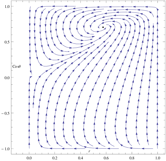
The determinant and the trace of the matrix A are, and respectively. For a matter dominated universe and . It is known that the fixed point is stable only when and . So is the condition for which the fixed point is stable. To draw the phase portrait of the system, we have plotted against instead of for . From the phase plot(figure 2.1) it is clear that the fixed point is stable in nature. So any solution of the system around this fixed point will be a stable solution for a wide range of initial values. It is clear from the phase plot that and are two invariant sub-manifolds. Here we have considered a local subspace bounded by invariant sub-manifold and . It also deserve mention that () is a saddle fixed point for our choice of parameter . The value of has been restricted between 0 and 1 from the physical requirement that and .
2.3.3 Examples with specific potentials
To study the system near the fixed point with tracking we consider two specific types of potentials as examples. Among many possibilities r21, we choose hyperbolic potential of the form where and are constants and exponential potential of the form , where , are positive constants and is the quintessence scalar field.
(i)
The tracking parameter and the parameter in this case are given by
and
respectively. If the quintessence field density tracks the background matter density then . A near tracking scenario can be achieved by assuming , where is very small. This would imply , i.e, scalar field has a very high value. As is very small we have neglected the higher powers of . The parameter will have a near constant value as for , . So can be written as .
| (2.17) |
and also
| (2.18) |
From the definition of and (equation( 2.7)), one can write and H as
| (2.19) |
| (2.20) |
where and B is arbitrary integration constant.This last equation can be utilized to write the deceleration parameter
as
| (2.21) |
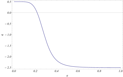
Now using equation( 2.21) ‘q’ can be plotted against ‘a’ (in units of , the present value of a). As we are looking for a tracking solution, , i.e. , so ‘’ is severely restricted. With the help of the equation (2.19) and the tracking condition, one can estimate the constant to be and . For a matter dominated universe i,e. , yields a ‘q’ which at least qualitatively resembles the present acceleration which is an observational quantity (see figure2.2 ). The problem is that the acceleration sets in quite early in the matter dominated era (near z=4). The other value, , predicts an acceleration at a distant future and hence not discussed.
(ii)
In this case and . To satisfy tracking condition, , is only one option. This condition also would imply has a near constant value. Near the fixed point and , it can be shown that
| (2.22) |
and
| (2.23) |
Here B is an integration constant and . The deceleration parameter ‘q’ can be written as
| (2.24) |
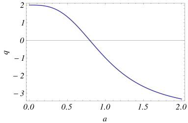
By considering present value of deceleration parameter ‘q’ and , the integration constant B can be expressed in terms of A and as . If we take k=1 and a matter dominated universe then . Plot of q vs for this potential agree well with the present accelerated expansion of the universe (see figure: 2.3).
2.3.4 Discussion
The stability of tracking quintessence models for the universe has been investigated in the present section. With a general tracking condition, the fixed point solutions are not too many. In fact there is one physically relevant generic fixed point, with tracking conditions, leading to a stable solution. The condition for stability, in terms of the fractional rate of change of the quintessence potential, is found out to be where .
Two specific potentials, giving rise to the present acceleration, are worked out as examples. It is found that for , the scalar field is severely restricted to a zone such that is close to unity. For the other example, , the conditions do not restrict the scalar field, but rather fine tunes the constants in the potential(eg. must have a very small value).
2.4 Quintessence Scalar Field: With Tracking Condition Relaxed
This section deals with the study of the possible stable solutions for some quintessence models when the tracking condition is relaxed. There is a host of quintessence potentials with some merits for each of them. For a comprehensive review, refer to( r21). Two well known potentials will be used as examples in the present work. The autonomous system of equations (2.8,2.9 and 2.10) is a three dimensional one for a general potential . For the exponential potential, the system effectively reduces to a two dimensional one as is constant. Where as the system is actually three dimensional for a power-law potential. The numerical solutions are found out. Some of the fixed points are non-hyperbolic so the stability of these fixed points can not be analysed by using linear stability analysis. The stability of these non-hyperbolic fixed points is analysed with a different strategy, namely by a small perturbation around the fixed point.
2.4.1 Estimation of boundary values:
From equation (2.3) the deceleration parameter can be express in terms of and as
| (2.25) |
For a spatially flat universe,
| (2.26) |
which, in view of the constraint equation (2.2), is restricted as
| (2.27) |
where is cold dark matter energy density parameter. This implies .
As the dark matter is expected to be cold, the subsequent discussion assumes that the corresponding pressure to be zero which implies . The numerical solutions for the system can be found out by fixing the boundary values. The boundary values of etc has been estimated using the present ( i.e., at ) values of etc as suggested by observations. Present observational value of , so
| (2.28) |
where and are the present values of and respectively. Using equation (2.28) in equation (2.25), a lower bound is set for present value of deceleration parameter () so as to make real.
To make it consistent with observations (see ref.r29 and references therein) and the lower bound of the deceleration parameter set for the present work, we set , then equations (2.25) and (2.28) would yield and . From the definition of , it is easy to check that when the potential is an exponential function of and for other values of , the potential has the form of power law. The present value of has been chosen to fit the observational results. Interestingly the numerical solutions evolve from a fixed point (asymptotic as ) of the system and attracted towards another fixed point (asymptotic as ) of the system. The solutions are heteroclinic orbits in phase space as they connect two different fixed points. Thus, the beginning and the ultimate fate of the universe can be qualitatively investigated by finding the behaviour of the fixed points.
2.4.2 Examples with specific potentials:
(i) Exponential Potential:
When , the definition of indicates that the potential has the form
| (2.29) |
where A and are constants. From equation (2.10), is a constant. So effectively the system becomes a 2-dimensional one.
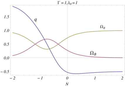
By numerically solving the equations (2.8) and (2.9), the plots for and are obtained. Plots for observationally relevant cosmological parameters have also been obtained. For these plots, we have taken . This also yields . It has been checked that for some other values of the analysis is possible, but there is hardly any qualitative difference, so we do not include them.
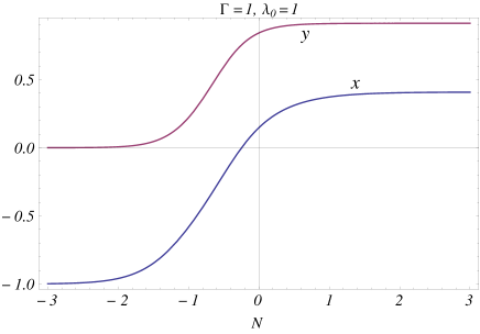
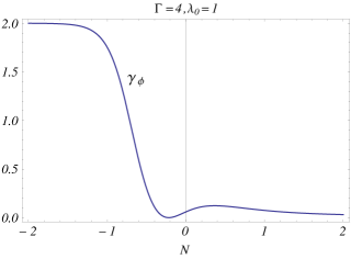
Figure (2.4) shows the evolution of against . The plots of cosmological parameters and against are shown in figure (2.5). The fixed points() of the system when and are (1.224,-1.224), (0.408,-0.912), (1,0), (-1,0), (1.224,1.224), (0.408,0.912) and (0,0). From figure (2.4), it is easy to find out the asymptotic behaviour of the system. We see that () is asymptotic to (-1,0) as in the past and to (0.408,0.912) as in the future. Determinant() and trace() of the Jacobian matrix at (-1,0) are and . As both these are positive, the point (-1,0) is an unstable fixed point. Determinant() and trace() of the Jacobian matrix at (0.408,0.912) are and , so this point is a stable fixed point. The fixed point (-1,0), which is past time attractor of our solution has the qualitative features like as . The qualitative features of the fixed point (0.408,0.912), which is a future time attractor, are and as .
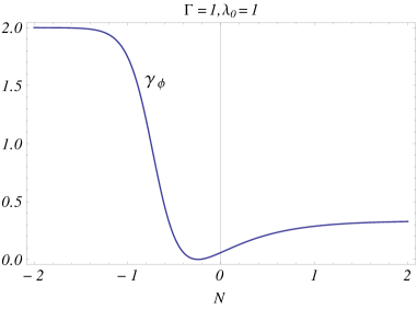
This analysis, along with reasonable boundary values (i.e. those indicated by observations) allows us to qualitatively study the beginning and the possible ultimate fate of the universe. It is seen that the present accelerated expansion is indeed a stable solution for the universe with an exponential potential for the quintessence scalar field. As the fixed point is an unstable fixed point thus, given a small perturbation from it, the universe evolves from the state when the linear size () was zero, the value of the scalar field infinity and the potential was zero. As the solutions connects two different fixed points thus, the solutions form heteroclinic orbits in phase space.At the beginning it expanded very rapidly () but at a decelerated rate. After this phase of decelerated expansion the universe has entered in to an accelerated expansion phase which is shown in figure(2.5). The accelerated expansion starts at about , which is quite consistent with the observations. From figure (2.5) , it is also seen that in recent past , but in remote past, dominates over though at that time the universe was undergoing a decelerated expansion.This is indeed intriguing. We see that in the remote past ( figure 2.6) and the pressure and the density of the quintessence field are related as . This indicates that the contribution to the pressure sector from the quintessence field had been positive and hence the quintessence field failed to drive an acceleration. But as the universe evolves, the value of drops below unity and the effective pressure becomes negative so as to drive an accelerated expansion.
As the universe asymptotically approaches the fixed point (0.408,0.912), so the future behaviour of the universe in this model can be described by qualitatively analysing it. This fixed point is a future time attractor as discussed before. So as , the universe settles to a state where and attains a constant value. The universe expands with a nearly constant acceleration.
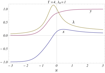
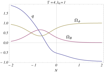
(ii) Power law type potentials: When , a constant but , the form of the potential can be found out from definition of as
| (2.30) |
where A,B and m are constants. In this case has a dynamics. It is not necessarily a constant, and we plot (fig 2.7) and also the cosmological parameters like (fig: 2.8 and 2.9 respectively), all against . As an example, we take . The fixed points () of the system for power law type potentials are (-1,0,0), (0,0,0), (1,0,0), (0,-1,0) and (0,1,0). These fixed points are independent of . From figure 2.7 we see that () curves are asymptotic to (-1,0,0) as and asymptotic to (0,1,0) as . The eigenvalues of the Jacobian of the system at (-1,0,0) is (3,3,0) and those at (0,1,0) is (-3,-3,0). As these fixed points are non-hyperbolic, we can not use linear stability analysis. The fixed point (-1,0,0) has two positive eigenvalues and one zero eigenvalue so it is an unstable fixed point. However, the fixed point (0,1,0) has two negative eigenvalues and one zero eigenvalue, so its being a stable fixed point cannot be ruled out before further investigation.
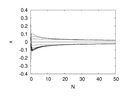
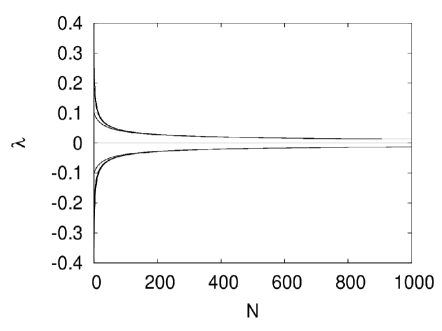
In order to check the stability of the latter fixed point, we perturb the system in every direction near the fixed point and numerically solve the system of equations to find its asymptotic behaviour as . The 3D phase portrait looks obscure and it is difficult to figure out the behaviour. So we have plotted and against in figure 2.10, 2.11 and 2.12. From figure 2.10, we see that approaches as . Also from figure 2.11 and figure 2.12, one concludes that y(N) approaches and approaches respectively as . So the system approaches the fixed point (0,1,0) as against perturbation near (0,1,0). The fixed point is thus a stable one. Thus, for a power law type potential also, a qualitative analysis can be looked at.
The universe evolves from the unstable fixed point (-1,0,0) representing the physical state ( constant and finite, ). As it is an unstable state, a small perturbation starts the evolution. After a long stint of decelerated expansion, the system enters into the phase of accelerated expansion and is attracted towards the stable fixed point (0,1,0). This final stable state will correspond to the physical state ( constant, constant) and it will expand with a nearly constant acceleration (figure 2.8).

2.4.3 Discussion:
This present section deals with a dynamical systems analysis of a quintessence scalar field that drives the recent accelerated expansion of the universe. An exponential potential and a power law type potential are worked out as examples. The boundary values of and are estimated from the recent observations and the boundary value of is chosen so that the result is consistent with the present observations. In both cases, it is possible to find a scenario where the universe in fact starts from an unstable fixed point (hence apt to move away from that) and evolves to a future attractor through the present phase of accelerated expansion. Amongst the several possible fixed points, only those are chosen which are past and present asymptotes for the set of solutions.
The observational value of density parameters of quintessence scalar field and background fluid are and respectively. This, in fact, is put into the system as a boundary value. It is intriguing to note that evolution suggests that actually dominates over its dark matter counterpart in the past as well except for a brief interval in the recent past. This feature is there for both the examples, i.e., an exponential or a power law potential. The reason that the universe decelerated in the past is the fact that the equation state parameter had been more than unity so that the quintessence field could not generate the all important negative pressure.
Both the examples lead to a situation where the universe in future will be governed completely by the quintessence field ( and ) and will be steadily accelerating. Although we have worked out for two examples, it appears from equation(2.10), the method can, in principle extended for any potential for which can be expressed as a function of .
It is important to note that a small change in the initial conditions does not inflict any major or qualitative change in the system. For instance, the system does not show any chaotic behaviour. This has been carefully checked.
Chapter 3 Stability of chameleon scalar field models
3.1 Introduction:
Theoretically mass-less scalar fields are abundant in string theory and supergravity theory. But these mass-less scalar fields predict very large violation of the Equivalence Principle(EP), which is physically unacceptable. Another interesting observational fact from the measurement of absorption line in quasar spectra is that the evolution of the fine structure constant is of the order of one part of over the redshift interval webb. To model a time varying coupling constant with a rolling scalar field the mass of the scalar field has to be of the order of present value of Hubble parameter ().
In justin1; justin2 , Khoury et al introduced the concept of chameleon scalar field . Unlike the common non-minimally coupled scalar field theories, a chameleon field is coupled to matter sector rather than the geometry. As a consequence of this the scalar field acquire a mass whose magnitude depends on the ambient matter distribution. In a region of high density, such on Earth, the mass of the scalar field is very large and the EP violations are suppressed. But in a region of very low density i.e. on cosmological scale the mass of the scalar field can be of the order of . So in cosmological scale the field can satisfy the bound on the violations of EP khoury. This change of properties of the field acts as a buffer in connection with the observational bounds set on the mass of the scalar fields coupled to the matter sector mota1.
A strongly coupled chameleon scalar field has the possibility of being detected by carefully designed experiments mota2; shaw1. Possible effect of the chameleon field on the cosmic microwave background with possible observational imprints has been estimated by Davis, Schelpe and Shaw shaw2 and that on the rotation curve of galaxies by Burikham and Panpanich buri. One very attractive feature of a chameleon field is that if it is coupled to an electromagnetic field brax1 in addition to the fluid, the fine tuning of the initial conditions on the chameleon may be resolved to a large extent mota3. The remarkable features of the chameleon field theories are comprehensively summarized by Khoury khoury.
Brax et al used this chameleon field as a dark energybrax. This kind of interaction between the dark matter and the dark energy was investigated in detail by Das, Coarsaniti and Khourydas in the context of the present acceleration of the universe. It was also shown that with a chameleon field of this sort, it is quite possible to obtain a smooth transition from a decelerated to an accelerated expansion for the universenbsdkg.
The success of the chameleon field in explaining the current accelerated expansion and its lucrative properties which open up the possibility to evade a fine tuning of initial conditions, and its possible observational imprints inevitably attracted a lot of attention. The possibility of a scalar field nonminimally coupled to gravity, such as the Brans-Dicke scalar field, acting as a chameleon was discussed by Das and Banerjee sdnb. Brans-Dicke scalar field acting as a chameleon with an infrared cut-off as that in the holographic models was discussed by Setare and Jamil jamil. The field profile of a chameleon was discussed by Tsujikawa, Tamaki and Tavakol tavakol.
The aim of the present chapter is to thoroughly investigate the stability criteria of the chameleon models in a spatially homogeneous and isotropic cosmology. There are two arbitrary functions of the chameleon field to start with, namely and . Here is the dark energy potential and determines the coupling of the chameleon field with the matter sector. We broadly classify the functions into two categories, exponential and non-exponential. So there are four combinations in all. We investigate the conditions for having a stable solution for the evolution for each of these categories. We find that there are possibilities of finding a stable evolution scenario where the universe may settle into a phase of accelerated expansion. However, if both and are exponential functions of , the stability is very strongly dictated by the model parameters. In fact it is noted that in this latter case there is a possibility of a transient acceleration at the present epoch but the final stable configuration of the universe is that of a decelerated expansion.
The method taken up is the dynamical systems study. The field equations are written as an autonomous system and the fixed points are found out. A stable fixed point indicates a sink and thus marks the possible stable final configuration of the universe whereas an unstable fixed point, indicating a source, may describe the possible beginning of the evolution. Application of dynamical systems in cosmological problems, mostly for scalar field distributions, is already there in the literature gunzig. For detailed discussions on some early work on such investigations, we refer to the monograph by Coley r13.
3.2 A chameleon scalar field:
The relevant action in gravity along with a chameleon field is given by
| (3.1) |
where R is Ricci scalar, G is the Newtonian constant of gravity, is the potential. Here is a function of the chameleon field and determines the non-minimal coupling of the chameleon scalar field with the matter sector which is given by . In what follows, is given by alone. This indeed is not a standard description. However, for a collection of collision-less particles with non-relativistic speed, the rest mass of the particles completely dominates over the kinetic energy, the contribution from the pressure is negligible compared to the rest energy. The density is defined to be the contribution to that by these collision-less particles. This is thus quite a legitimate choiceharko1; harko2 for a pressure-less fluid, which would be relevant for the dark matter distribution.
By varying the action with respect to the metric tensor components, one can find the field equations. For a spatially flat FRW spacetime given by the line element
| (3.2) |
the field equations are written as
| (3.3) |
| (3.4) |
where the units are so chosen that . The fluid is taken in the form of pressureless dust consistent with a matter dominated universe and is the matter density. Overhead dots denote differentiation with respect to the cosmic time .
By varying the action with respect to the chameleon field , one can also find the wave equation as,
| (3.5) |
| (3.6) |
which is actually the matter conservation equation. On integration, the equation (3.6) yields
| (3.7) |
All of these equations (3.3), (3.4), (3.5) and (3.6) are not independent. Any one of the last two can be derived from the other three as a consequence of the Bianchi identities. We take (3.3), (3.4) and (3.5) to constitute the system of equations. There are, however, four unknowns, namely . The other variable, , is known in terms of via the equation (3.7). It is intriguing to note that even with the nonminimal coupling with the scalar field, the matter energy density itself still redshifts as (see reference nbsdkg)
3.3 The Autonomous system:
By the introduction of following dimensionless variables
, , , , ,
and ,
the system of equations reduces to the following set,
| (3.8) |
| (3.9) |
| (3.10) |
| (3.11) |
| (3.12) |
A ‘prime’ indicates differentiation with respect to with chosen as unity. One can write equation (3.3) in terms of these new variables as
| (3.13) |
We use this equation as a constraint equation and the system which now effectively reduces to,
| (3.14) |
| (3.15) |
| (3.16) |
| (3.17) |
We now use standard linear stability analysis to qualitatively analyse the system. It can be seen that some of the fixed points are non-hyperbolic in nature. For non hyperbolic fixed points, one can not use linear stability analysis. In the absence of a proper analytical process, a different strategy in such cases may be adopted. The solutions are numerically perturbed around the fixed points to check the stability in non hyperbolic cases. If the perturbed solutions asymptotically approach the fixed points, the corresponding fixed points are considered stable. This approach is quite standard in nonlinear dynamicsr19 and has already been utilised quite recently in a cosmological scenarionrnb.
3.4 Stability analysis of the chameleon model:
From definition of and , it can be easily shown that corresponds to the exponential form of the potential and corresponds to exponential form of the coupling. For the sake of making the system of equations a bit more tractable, we classify our system into four classes as described below.
Class I : When and , i.e., both the potential and the coupling are non-exponential functions of the chameleon field.
Class II : When and , the potential is an exponential function of the chameleon field but the coupling is any function of the chameleon field excluding an exponential function.
Class III: When and , the potential is any function excluding an exponential function but the coupling is an exponential function of the chameleon field .
Class IV : When and , both the potential and the coupling are exponential functions of the chameleon scalar field .
3.4.1 Class I :When both the potential and the coupling with matter are non exponential functions of the chameleon field.
In this class, the system formed by the equations (3.14), (3.15), (3.16) and (3.17), has the fixed points as listed in Table 3.1.
| Points | |||||
| 0 | 0 | 0 | -1 | +1 | |
| 0 | +1 | -1 | 0 | 0 | |
| 0 | 0 | 0 | |||
| 0 | 0 | 0 | 0 |
In order to study the stability of the fixed points, the eigenvalues of the Jacobian matrix have been found out for all the fixed points which are shown in Table 3.2.
| Points | ||||
| 0 | 0 | |||
| 3 | 0 | 0 | ||
| 3 | 0 | 0 | ||
| 6 | 0 | 0 | ||
| 6 | 0 | 0 |
As the Jacobian matrix of the fixed points all have at least one zero eigen values, these are all non hyperbolic fixed points. One can not use the linear stability analysis in this situation. Fixed points and has at least one positive eigenvalue, so these fixed points are in fact unstable but the one at has two negative eigenvalues and two zero eigenvalues and thus requires further investigation. It must be made clear that is actually an infinite set of fixed points as the value of is arbitrary in this case, as indicated in Table 3.1. We perturb the system around the fixed points . It is not possible to draw a 4D phase plot and the 3D phase plot looks too obscure to draw conclusions from. We adopt the following strategy. We plot the projection of perturbations on and axes separately. In figure 3.1, the whole line corresponds to the fixed point. For a small perturbation of the solution around the fixed point , the evolution of the solution with is studied numerically. It is evident from figure 3.1 that the perturbed solutions asymptotically approach as . Figure 3.2 and 3.3 show that the projection of perturbations around and approaches and respectively as . It is interesting to note that the results given by this perturbation technique is completely consistent with the finding that is arbitrary. Any perturbation of the system around any value of renders it remaining constant at the perturbed value without any further evolution (figure 3.4). From this behaviour of the system near , we can conclude that axis is an attractor liner19.
Any heteroclinic orbit in the phase space of the system starts from an unstable fixed point and ends at a stable fixed point. So the universe is apt to start evolving from one of these unstable fixed points to as a result of any small perturbation and approach towards the axis which is an attractor line as .
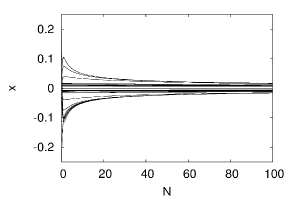
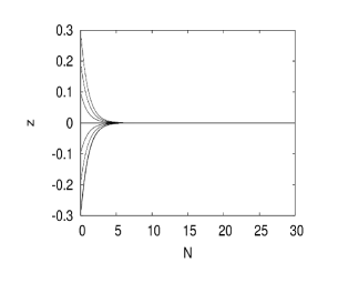
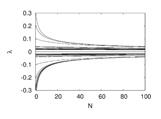
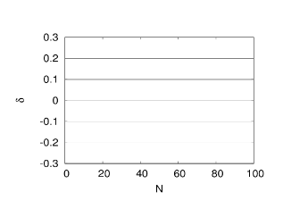
The set of fixed points , given by with an arbitrary , is thus stable (an attractor) and gives the final state of the universe. The physical state of the universe in this case, as (i.e., ), is consistent with . Here we define and .
It deserves mention that as , the contribution from the kinetic part of the chameleon goes to zero and this complete domination of the chameleon field is entirely given by the potential part. From equation (3.4), one can see that the universe settles to an accelerated phase with .
The unstable fixed points and indicate states with and . This is consistent with the physical requirement of the early phase of the evolution. However the fixed point will henceforth be disregarded as unphysical, as for a positive , negative values of do not represent any physical state.
Like , the other two fixed points and are also unstable fixed points and describe physical states with the relative magnitude of and being reversed. However, it also deserves mention that for both and , remains positive (equal to ) and thus the scalar field does not really play the role of a dark energy. It deserves mention that and as given by figures 3.1 and 3.3 might appear to be leading to a non-zero constant value. But the ordinates are not really parallel to the horizontal axis, they do vary, but only too slowly. It is checked that they indeed approach zero for a very large value of .
3.4.2 Class II: When the potential is an exponential function of the chameleon field but the coupling with matter is any function of the chameleon field except an exponential one:
In this class is a constant and equations (3.14), (3.15) and (3.17) form the system of equations. The fixed points of the system are given in Table 3.3 and the eigenvalues of the Jacobian matrix at the fixed points are given in Table 3.4.
| Points | ||||||||
| x | 0 | 0 | 0 | +1 | -1 | |||
| z | 0 | +1 | -1 | 0 | 0 | 0 | ||
| 0 | 0 | 0 | 0 | 0 | 0 | 0 |
| Points | |||
| 0 | |||
| 3 | 0 | ||
| 3 | 0 | ||
| 3 | 0 | ||
| 3 | 0 | ||
| 0 | |||
| and | 0 |
Here the symbols, and , are used for brevity.
Existence of the fixed point at demands , indicating that is a constant in this case. This could have a bearing on the chameleon mechanism. This is a non isolated fixed point and has one zero eigenvalue at each point, defined by the value of , of the equilibrium set. These type of fixed points are called normally hyperbolic fixed points (r13). The stability of a normally hyperbolic fixed point depends on the signatures of the remaining eigenvalues. If sign of the remaining eigenvalues are negative then the fixed point is a stable fixed point otherwise the fixed point is an unstable one. For , the remaining eigenvalues are and , so is a stable fixed point.
Other fixed points are non hyperbolic and not even normally hyperbolic. The fixed point can have one zero eigenvalue and two negative eigenvalues if whereas can also have one zero eigenvalue with two negative eigenvalues if . So in the corresponding parameter range and need further investigation as in case of Class I type of models. It is found that for a small perturbation about these fixed points (, and ), the solutions do not approach towards the fixed points as , so these fixed points are unstable. The fixed points and are also unstable fixed points as they have at least one positive eigenvalue. So to could be the beginning of the evolution and may be the possible ultimate fate of the universe. It also deserves mention that for , is in fact a subset of . It is interesting to note that for , the fixed point is realized only for . The fixed points and are not analysed on the plea that for a negative , the state is not physical as it corresponds to a negative value of .
Amongst the fixed points, potentially the beginning of the universe (i.e., unstable fixed points), and has the possibility of and which is a desired situation. The only stable fixed point, , yields the possibility of a final fate where and with .
3.4.3 Class III :When the coupling with matter is an exponential function of the chameleon field but the potential is any function of the same except an exponential function:
When the coupling of the chameleon with the matter field is an exponential function of , one has constant. The system of equations is formed by equations (3.14), (3.15) and (3.16). Fixed points of the system are given in Table 3.5 and the eigenvalues of the Jacobian matrix at the fixed points are given in Table 3.6.
| Points | |||||||
| x | 0 | 0 | 0 | 1 | -1 | ||
| z | 0 | 0 | 0 | ||||
| 0 | 0 | 0 | 0 | 0 |
| Points | |||
| 0 | |||
| 3 | 0 | ||
| 3 | 0 | ||
| 6 | 0 | ||
| 6 | 0 | ||
| 0 | |||
| 0 |
The existence of fixed point requires the condition that indicating that is a constant! This would require that the nonminimal coupling between the chameleon field and matter becomes trivial and certainly there is a breakdown of the chameleon mechanism. Unphysical states (negative values of ) given by the fixed points and are not discussed.
Fixed point has one zero eigenvalue and two negative eigenvalues. It is a non hyperbolic fixed point and thus one can not use the linear stability analysis in this case. So we perturbed the system from the fixed point and numerically solved the system of equations for each perturbations. Plots of the projections of the perturbations on and against in figures (3.5), (3.6) and (3.7) show quite convincingly that for large , the solutions approach the fixed point which is thus an attractor. So is apt to represent the final state of the evolution.
Other fixed points are unstable. In the beginning, the universe could be at any of these unstable fixed points and with a small perturbation from these unstable fixed points might start evolving towards the attractor which can be the possible final state of the universe for which and are evident possibilities. The final stage is completely dominated by the potential which is a constant, effectively giving a cosmological constant, with .
Amongst the unstable fixed point, is definitely favoured as they indicate and for the initial epoch. For the unstable fixed points and , although , the chameleon cannot act as a dark energy as is not negative. The fixed point will indicate a matter dominated early epoch if and could well be amongst the viable options. Like Case I, in this case also, and actually approach zero which had been revealed on an extension of the horizontal axis, roughly up-to 1000.


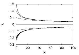
3.4.4 Class IV :When the potential and the coupling with matter both are exponential functions of the chameleon field :
In this class of the model both and are constants. Equations (3.14) and (3.15) constitute the system of equations for the effectively two-dimensional problem. The fixed points of the system are given in Table 3.7.
| Points | |||||||
| x | -1 | 1 | |||||
| z | 0 | 0 | 0 |
This is a 2D system, so the stability of the fixed points can be checked by both the methods, like from sign of eigen values of the Jacobian matrix or from trace and determinant of the Jacobian matrix at the fixed point. Depending on the degree of simplicity they offer, one of these two methods are used for different fixed points. There are seven fixed points, to . We analyse the stability of the fixed points to by the signature of the eigenvalues of corresponding Jacobian matrix (see Table 3.8). For and , the trace and determinant of the Jacobian matrix are looked at. For the present case when both and are exponential functions of , both of and are constants and the fixed points are found in terms of these two constants of the theory. The stability criteria crucially depend on the values of and . Depending on the values of these two constants, there are special cases. One of them, namely with , which results in , has an interesting feature that it actually coincides with and . This fixed point will be taken up in the last section.
| Points | Conditions of stability | ||
Trace and determinant of the Jacobian matrix at and are and respectively. Conditions for stability of and are,
1. .
2. .
3. .
4. .
5. .
6..
The fixed point is irrelevant as it requires a negative and thus a negative and is relevant only in cases where is negative for the same reason. In what follows, an example of an unstable and that of a stable fixed point of this class are given. We choose and the deceleration parameter r29 in order to pick up some relevant values of the model parameters and . With this value of , it is easy to see from the definitions of and that and thus from the constraint , one has , i.e., . From the field equations (3.3) and (3.4), one can write
| (3.18) |
which yields . Now from the Table 3.7, Table 3.8 and list of the stability conditions of and , one can check that for and , one has as an unstable fixed point and as a stable one. So the universe is apt to start its evolution from and settle into a final configuration at . The behaviour of against and that of the cosmological parameters , , and against are given in figures 3.8 and 3.9 respectively. It is easy to check that the universe starts with a deceleration () but with and and settles down to final phase of decelerated expansion with and again the same state of and . There is an accelerated expansion in between, around the present stage of evolution (see figure 3.9). So this is a nice example of a transient acceleration.
As this case effectively reduces to a 2-dimensional problem, one can draw the phase plot in and , for the given values of and , 1.8 and -0.1 respectively. The plot is shown in figure 3.10. In figure 3.11, we zoom the plot around in order to understand the stability a bit more clearly.
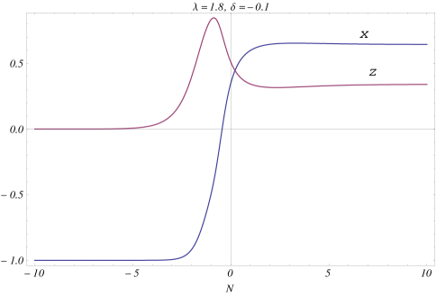
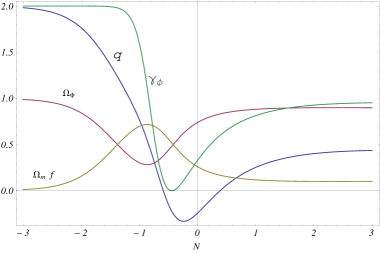
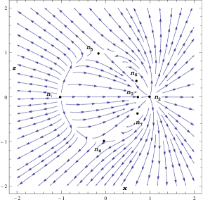
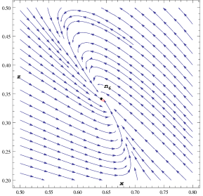
3.5 Chameleon mechanism and acceleration of the universe
Khoury discussed the restriction of the mass of the chameleon field vis-a-vis the coupling of the chameleon field with matter considering the compatibility of adaptation of the chameleon with the ambience and the requirement of the laboratory based experimentskhoury. The example taken up is the one for which and . Here and are constants and determines the strength of the coupling . The allowed band in the vs plot was worked out.
The example is clearly in the Class I of the present work where both of and are non-exponential functions. In this case and , both are independent of . As an illustration, we take up the case for . With the boundary values of , chosen from observational constraints as in section 3.4.4, one can plot the variables and (figure 3.12). The plot of the deceleration parameter against (figure 3.13) shows that the universe has a smooth transition from a decelerated to an accelerated expansion approximately at which corresponds to a red-shift of 0.74, which perfectly matches the observationob. So we find one example where this transition happens independent of the coupling of the scalar field with matter and hence posing no threat to the allowed band between and the mass of the scalar field. It also deserves mention that the system has evolved from an unstable fixed point and approaches to a stable fixed point , which also agrees very well with the present dynamical systems analysis of Class I models.
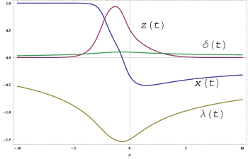
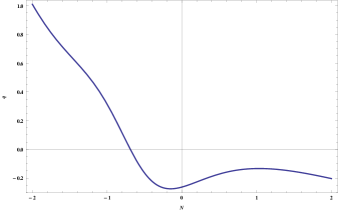
3.6 Discussion
The stability of the various chameleon scalar field models are investigated in the context of the present accelerated expansion of the universe in the present chapter. The aim is not to suggest any new model of dark energy, but rather to look at the various possibilities where a chameleon field can indeed serve as driver of the acceleration, starting from a decelerated situation. An unstable fixed point might describe the initial stage of the universe from where a small perturbation could trigger the start of the evolution whereas a stable fixed point is apt to describe the final stage of the universe. Unlike many of the dark energy models, a chameleon field has the distinct possibilities of being detected and hence that of being nullified as well. Thus it warrants attention regarding the choice of the favoured combination of the dark energy potential and the coupling with matter.
For the sake of convenience, the functions and are classified as either exponential or not. So in all there are four such combinations, which are quite extensively studied in the present work. In fact any old (or new) chameleon model with given and , the stability criteria need not be checked afresh. The present investigation provides a complete set of choices for and and can serve as the diagnostics.
It has been mentioned in Section 2.2 that there are actually four unknown quantities, namely and . In class I unknown and the autonomous system is 4 dimensional. Class II and III have one of and exponential and the system reduces to a 3-dimensional one. Class IV has both of and exponential and the system reduces to a 2-dimensional problem. The autonomous system is thus verified to be consistent with the number of unknowns.
It is found that if both and are exponential functions, and are not dynamical variables but are rather some parameters. The stability of the fixed points depends on the values of these parameters and it opens up a possibility for a transient acceleration for the universe around the present epoch. The other observation is that when is exponential and is not, effectively resembles a cosmological constant and when is exponential but is not, the matter-chameleon coupling is actually broken.
It is interesting to note that the fixed point with and , and are in fact the same, where there is no fluid and the scalar field sits at a non-zero minimum. So all the different combinations of and coincide at this fixed point which formally resembles a de Sitter model.
We can also find at least one example where the cosmological observations of the transition from the decelerated phase to the accelerated one can happen without any contradiction with the allowed band between the mass of the scalar field and its coupling with matter.
As already mentioned, the basic aim was not to propose a new chameleon model but rather to provide an exhaustive study of the stability characteristics of all possible combination of and . This purpose is achieved quite comprehensively and as a bonus some interesting physical features are also noted. For example, it is noted that a chameleon field can give rise to a transient acceleration for the universe and certain combination of the potential and the coupling leads to a breakdown of the chameleon mechanism itself.
Chapter 4 Stability analysis of a holographic dark energy model
4.1 Introduction:
Holographic principle was proposed by Gerard ’t Hooft and Leonard Susskind 'thooft; susskind. According to the holographic principle, the degrees of freedom of any system is determined by the area of the boundary and not really by the volume. It was originally inspired by black hole thermodynamics. The principle states that the surface fluctuations of the event horizon of a black hole contain description of all the objects ever fall in. Mathematically, the energy inside a region of length , must not exceed the mass of a black hole of the same size. From effective field theory , where is the infra-red cut-off and this has to be a cosmological length scale if we consider cosmological holography. In cosmological holography the universe can be thought of as a two dimensional information structure painting on the cosmological horizon. There are three different choices of , the Hubble radius, the particle and the event horizon and Ricci scalar curvature. The dark energy models in which the cut-off length is identified with the Hubble radius () Cohen, calculated dark energy density is close to the observed effective cosmological constant. Li in li discussed that considering the particle horizon and the event horizon as the cut-off length scale, it is possible to construct viable dark energy models. The cosmological dynamics of the Ricci dark energy models, in which the length scale is identified with the Ricci scalar is discussed in Gao; Camco.
Pavon in diego, gave a brief but comprehensive review of this infra-red cut-off and its application in cosmology as a “holographic” dark energy. Cosmological implications of this holographic dark energy, particularly its role in driving the accelerated expansion of the universe have been quite thoroughly discussedli; diego1; diego2. Holographic dark energy has been discussed in non-minimally couple theories as well, such in Brans-Dicke theory by Banerjee and Pavondiego3, and in a chameleon scalar field model by Setare and Jamilsetare.
The holographic dark energy attracted attention as it can alleviate, if not resolve, the issue of cosmic coincidence, i.e., why the energy densities due the dark matter and the dark energy should have a constant ratio of order unity for the present universediego2.
This chapter deals with the stability of a holographic dark energy model in standard Einstein’s gravity. The model is quite general as it allows interaction between the dark energy and the dark matter, so that one can grow at the expense of the other. The dynamical systems analysis has been used to study the system . The field equations are written as an autonomous system and the fixed points are found out. A stable fixed point, an “attractor”, is likely to describe the final state of the universe. As already mentioned, this kind of dynamical systems study is not new in cosmology. There are excellent reviews on this topicr13. However, such analysis is more frequently used where a scalar field is involved. A few dynamical systems study on holographic dark energy models, such as one where the infra-red cut-off given by the Ricci lengthnairi1 and by the future event horizonnairi2 are there in the literature. Setare and Vagenassetare1 discussed the bounds on the effective equation of state parameters on the basis of dynamical systems study, with an infra-red cut off given by the future event horizon. The present deals with a holographic dark energy model where the cut-off is determined by the Hubble lengthdiego; diego2.
4.2 Phase space analysis of the model:
We consider an interacting holographic dark energy model in which the universe is filled with a pressureless matter component with energy density and a holographic dark energy of density . There is an interaction between these two components. The total energy density of the universe is .
In a spatially flat FRW universe with the line element
| (4.1) |
Einstein’s field equations are
| (4.2) |
| (4.3) |
where , is the equation of state parameter of holographic dark energy, is the contribution to the pressure by the holographic dark energy and , is the ratio of the two energy densitiesli; diego.
The conservation equations for and are
| (4.4) |
and
| (4.5) |
respectively. The dark matter and the dark energy are assumed to interact amongst themselves and hence do not conserve separately. They conserve together and is the rate of loss of one form and hence the gain of the other and is assumed to be proportional to the dark energy density given by , where is the decay ratediego1.
If the holographic bound is saturated, one hasli
| (4.7) |
where is the infra-red cut-off that sets the holographic bound. The Plank mass is given by . If the cut-off is chosen to be the Hubble length, which has a possible contribution towards the resolution of the coincidence problemdiego1, one has
| (4.8) |
| (4.9) |
Equations (4.5) and (4.9) yield the expression for the equation of state parameter for the holographic dark energy as,
| (4.10) |
From equations (4.7) and (4.2), one has . Considering a saturation of the holographic dark energy, equations (4.3) and (4.5) now yield
| (4.11) |
and,
| (4.12) |
In the subsequent discussion, equations (4.11) and (4.12) will replace the field equations (4.2) and (4.3). For the study of the phase space behaviour of the system, we introduce a new set of variables , and . The system of equations can now be written in the form of an autonomous system in terms of new dynamical variables as
| (4.13) |
| (4.14) |
Here and a ‘prime’ indicates a differentiation with respect to , where . In an FRW cosmology, , the fractional rate of change of the length scale of the universe, is the naturally available rate. We assume the decay rate to be a function of , . Depending on the value of , we have classified our system into two classes.
I) When , is any function of , except a linear function.
II) When , is linear functions of H.
4.2.1 Class I:
In this case the problem is a two-dimensional one and equations (4.13) and (4.14) form our system. Fixed points of the system are the simultaneous solutions of the equation and . So it is easy to check that it admits two fixed points, namely, and is arbitrary, . The second fixed point is a set of non isolated fixed points, a straight line parallel to - axis. If Jacobian matrix at any point of a set of non isolated fixed points has at least one zero eigenvalue the set of fixed points is called normally hyperbolicr19. Stability of a normally hyperbolicreza set of fixed points can be analysed from sign of remaining eigenvalues. If remaining eigenvalues are negative then the fixed point is stable. Eigenvalues and stability condition of the fixed points are given in the following table.
| Fixed Points | Co-ordinate | eigenvalues | Condition of stability |
Phase plots of this system has been shown in figure 4.1 and figure 4.2 for and respectively. The plots show that fixed points and are indeed stable for and respectively. This is consistent with the fact that negative eigenvalues indicate stable fixed points (see table 4.1).
Form the field equations and the definition of and , the deceleration parameter can be written as
| (4.15) |
As we have two fixed points, the system may be treated as a heteroclinic one where solutions join two fixed points.
For , is a stable fixed point and is an unstable one, thus indicating a sink and source respectively. So the universe can originate from with an acceleration () and an arbitrary and can settle down to , the stable fixed point where the expansion is decelerated () with . This squarely contradicts the observation which indicates an exactly opposite situation!
For , however, the fixed points actually reverse their roles as the source and the sink. In this case is unstable, thus, for a small perturbation, the universe starts evolving with a deceleration () and settles down to the final configuration of an accelerated expansion (). The final is an arbitrary function of . This situation is indeed realistic.
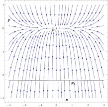
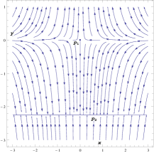
It deserves mention that is not actually a constant. So the figures 4.1 and 4.2 represents a section of the 3-dimensional figure at particular values of , i.e., snapshots at those values. If one changes the values of , the nature of the figures remain the same. For a particular value of , equations (4.13) and (4.14) lead to an expression for the deceleration parameter in terms of scale factor as, where is integration constant.
In figure 4.3 and 4.4, the evolution of the deceleration parameter against is shown where is the present value of the scale factor. It is clearly seen that is favoured in order to describe the observed dynamics of the universe. It should be noted that, for, , the interaction rate decays at a slower rate than the decay of and for a negative , the rate actually grows with some power of the decay of .
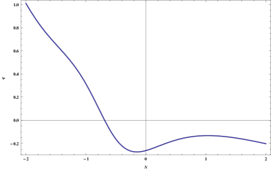
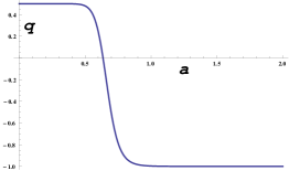
4.2.2 Class II :
In this case is a linear function of , given by . Our system of equations reduces to
| (4.16) |
| (4.17) |
As is a constant, this is essentially a one dimensional system with and , a constant. Integration of the equation (4.16) yields the solution for as where A is a constant of integration and . If , the solution is indeed stable, as for , one has . For , the fixed point is unstable. The phase plot is shown in figure 4.5, which indicates that the -axis is the attractor of all solutions for . Since is a constant, equation (4.15) indicates that there is no transition from a decelerated to an accelerated expansion for the universe.
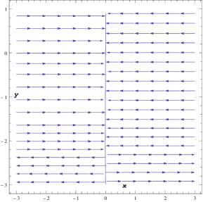
4.3 Bifurcation in the system:
It is interesting, from the point of view of the dynamical systems, to note that there is a clear bifurcation in the system, where is the bifurcation parameter and is the bifurcation point. When , there are two fixed points, and where is unstable but is stable. As approaches unity these two merge into a single fixed point where the stability depends on the choice of the values of the constants and . With , i.e., when it attains values on the other side of the bifurcation point, one has the same two fixed points with their roles interchanged so far as the stability is concerned. Figures 4.1,4.2 and figure 4.5 show the change of the behaviour of the phase space with variation of , which clearly indicate the occurrence of the bifurcation in the system. At the bifurcation point, , is a constant. As already mentioned, there is no transition from a decelerated to an accelerated expansion for the universe for a spatially flat FRW metric at bifurcation. This result is completely consistent with that obtained by Pavon and Zimdahldiego2.
4.4 Discussion
The holographic dark energy, tipped by many as the possible saviour from the coincidence problem, is analyzed as an autonomous system. It is found that the system indeed has unstable and stable fixed points. It is found that for , where , the system indeed has at least one natural description of the universe which starts with a decelerated expansion () and settles down to an accelerated expansion for the universe with dark matter completely giving way to the dark energy. So the interacting holographic dark energy warrants more attention, particularly when leading to . We see that the interaction rate actually plays a crucial role in this.
Chapter 5 Conclusion
In this thesis, we used a dynamical systems analysis to find the qualitative behaviour of some dark energy models. Specifically, quintessence scalar field models, chameleon scalar field models and holographic models of dark energy are discussed in the present thesis.
Einstein’s field equations form a set of nonlinear differential equations. So finding out an exact solution is not always easy. But, using a dynamical systems analysis the qualitative behaviour of the non-linear system can be investigated. Usually a set of suitable new variables and a dimensionless time variable are introduced so as to write the field equations as an autonomous system of equations. The fixed points of the system lead to the stability analysis of the system. Stable fixed points are the late time attractors and unstable fixed points are the repellers. Any heteroclinic solution of the system starts from an unstable fixed point and approaches to a stable fixed point. So one can study the beginning and possible ultimate fate of the universe by finding out the behaviour of the physical parameters near the fixed points.
In the second chapter, Quintessence scalar field models, with and without a tracking condition, are analyzed. In the first part, the qualitative behaviour of the system in the neighborhood of the fixed points is analyzed with a tracking condition, where the evolution of the scalar field almost mimics that of the matter field and picks up the dominant role very slowly in the later stage. This alleviates the so-called coincidence problem. It is found that, only one fixed point is of physical relevance in such a situation. Two specific forms of the potential are discussed, one is an exponential potential and the other is in a cosine hyperbolic form. It is also shown that each of them can drive the accelerated expansion of the universe near the fixed point.
In the second part, the tracking condition is relaxed, and with the boundary values consistent with the present observations, the system has been numerically evolved for two type of specific potentials to find the qualitative behaviour of the universe. It is found for both the potentials, one an exponential and the other being a power-law, the solution starts from an unstable fixed point and evolve to a stable fixed point. From this heteroclinic behaviour of the solution, a qualitative study of the beginning, present phase of accelerated expansion and possible ultimate fate of the universe has been carried out. It is intriguing to note that in both the examples, the scalar field energy density dominates over the dark matter density not only at present, but also at the beginning. With a favourable equation of state parameter () in the beginning, the effective pressure is positive leading to a decelerated expansion. The parameter evolves to a negative value only at a later epoch. So the model successfully drives a late time acceleration. However, this may encounter problems with other physical requirements such as Big Bang Neucleosynthesis.
The third chapter deals with the dynamical systems study of the Chameleon dark energy models. In Chameleon cosmology models the scalar field is non-minimally coupled to the matter sector and it’s effective mass depends on ambient matter density. Actually, this chapter provides an exhaustive diagnostic in terms of stability of the model for the combinations of all types of chameleon potential and its coupling with the matter sector. Phase space behaviour of each class has been investigated along with the nature and asymptotic behaviour of the fixed points.
In the fourth chapter, the field equations of a holographic dark energy model are written as an autonomous system and the standard dynamical systems analysis is done. Assuming the decay rate to be function of , the system is classified into two classes depending on the functional form of the decay rate. It is interesting to note that the system undergoes a bifurcation at a parametric value of . It is also found that when decay rate is a simple linear function of , there is no transition from decelerated expansion phase to the accelerated expansion phase of the universe.
Amongst the models discussed, there is hardly any pointer to pick up one as the most favoured candidate as a dark energy. But certainly the chameleon fields have the widest variety of possibilities.