Distributed Resource Allocation Over Random Networks Based on Stochastic Approximation

Abstract

In this paper, a stochastic approximation (SA) based distributed algorithm is proposed to solve the resource allocation (RA) with uncertainties. In this problem, a group of agents cooperatively optimize a separable optimization problem with a linear network resource constraint and allocation feasibility constraints, where the global objective function is the sum of agents’ local objective functions. Each agent can only get noisy observations of its local function’s gradient and its local resource, which cannot be shared by other agents or transmitted to a center. Moreover, there are communication uncertainties such as time-varying topologies (described by random graphs) and additive channel noises. To solve the RA, we propose an SA-based distributed algorithm, and prove that agents can collaboratively achieve the optimal allocation with probability one by virtue of ordinary differential equation (ODE) method for SA. Finally, simulations related to the demand response management in power systems verify the effectiveness of the proposed algorithm.

1 Introduction

Resource allocation (RA) problem is to allocate the network resource among a group of agents while optimizing certain performance index. It has drawn much research attention in many areas, such as the media access control in communication networks [1], signal processing in [2], and load demand management in [3]. Hence, various RA models and RA algorithms have been proposed (see [1]-[6] and the references therein). However, most of existing algorithms need a center to collect the data over networks or to coordinate computation processes among all agents.

In fact, the center-free distributed optimization algorithms have attracted more and more research attention in recent years [7]-[13]. In various network optimization problems, the optimal decisions are made based on the whole network data, which, however, are collected and stored by each individual agent of the network. The distributed optimization algorithm keeps the data distributed through the network when seeking the optimal decision, and hence eliminates the “one-to-all” communication burden and protects agents’ privacy. Distributed optimization also endows each individual agent with autonomy and reactivity by allowing it to formulate its local objective function and constraints with its local data. From the network viewpoint, the robustness to single point failure and the network scalability can be enhanced with distributed design. Following the seminal work [5] of RA in large-scale networks along with the distributed optimization work in [7]-[13], various center-free distributed algorithms for RA have been proposed recently in [14]-[17].

Stochastic approximation (SA) has been adopted in distributed optimization algorithms to address various kinds of uncertainties or to improve the computation efficiency. In [8], an SA-based distributed algorithm was proposed when each agent can only get the noisy observations of its local gradient, which extended the traditional SA optimization methods (see [18]) to distributed settings. In [19], an SA algorithm was given for distributed root seeking problem under noisy observations, which was also a generalization of distributed optimization problems. In practice, noisy gradient observations also exist in the zero-order distributed optimization algorithm as in [20], and randomized data sample was considered to reduce the computational complexity in optimization with “big data”, resorting to SA for theoretical analysis (see [21]). Besides, SA algorithms were also adopted for distributed optimization to handle uncertainties in communication systems in [9, 10], and [22].

Nevertheless, the existing distributed works of RA in [14]-[17] have not considered various stochastic uncertainties related to information sharing or data observations. Since the problem data is distributed throughout the network, each agent needs to share its local information with other agents through a communication network, which may involve various of uncertainties. Firstly, the communication network may switch due to packet loss, media access control, or energy constraint. To describe uncertainties of communication topologies, different from the deterministic switching graphs in [7, 12] and [13], we adopt random graph models like [9, 10, 23] and [24] here. Secondly, the information shared through the network may not be accurate or may be corrupted by random noises due to quantization errors or channel fading ( referring to [13], [22] and [24]). On the other hand, noises can also be actively added to the shared information for privacy protection as discussed in [25]. Moreover, agents may not get the exact local gradient or resource information due to measurement or observation noises.

Main contributions of the paper are summarized as follows. (i) A novel center-free distributed algorithm is proposed to handle the RA problem, where each agent only utilizes noisy observations of its local gradient and resource information, and noisy neighboring information shared through the randomly switching networks. (ii) The estimates are shown to converge to the optimal allocation with probability one based on the ODE method for SA algorithm. (iii) The proposed model and algorithm are applied to distributed multi-periods demand response management in power systems, along with simulations to show the effectiveness.

The remainder of the paper is organized as follows. The RA problem is formulated and an SA-based distributed algorithm is proposed in Section 2. Then the convergence result for the distributed algorithm is established in Section 3, while simulation studies are shown in Section 4. Finally, the concluding remarks are given in Section 5.

2 Problem Formulation and Proposed Algorithm

Firstly, we show related notations and preliminaries about convex analysis. Denote $\mathbf{1}_{m}=(1,...,1)^{T}\in\mathbf{R}^{m}$ and $\mathbf{0}_{m}=(0,...,0)^{T}\in\mathbf{R}^{m}$. $col\{x_{1},\cdots,x_{n}\}=(x_{1}^{T},\cdots,x_{n}^{T})^{T}$ stacks the vectors $x_{1},\cdots,x_{n}$. $I_{n}$ denotes the identity matrix in $\mathbf{R}^{n\times n}$. For a matrix $A=[a_{ij}]$, $a_{ij}$ or $A_{ij}$ stands for the matrix entry in the $i$th row and $j$th column of $A$. $\otimes$ denotes the Kronecker product. Denote $ker\{A\}$ and $range\{A\}$ as the null space and range space of matrix $A$, respectively.

For a nonempty closed convex set $\Omega\subset\mathbf{R}^{m}$ and a point $x\in\mathbf{R}^{m}$, denote $P_{\Omega}(x)$ as the point in $\Omega$ that is closest to $x$, and call it the projection of $x$ on $\Omega$. $P_{\Omega}(x)$ contains only one element for any $x\in\mathbf{R}^{m},$ and satisfies

$$\|P_{\Omega}(x)-P_{\Omega}(y)\|\leq\|x-y\|~{}~{}\forall x,y\in\mathbf{R}^{m}.$$ (1)

For a convex set $\Omega\subset\mathbf{R}^{m}$ and a point $x\in\Omega$, define the normal cone to $\Omega$ at $x$ as $N_{\Omega}(x)\triangleq\{v\in\mathbf{R}^{m}:\langle v,y-x\rangle\leq 0~{}~{}\forall y\in\Omega\}$.

In the following two subsections, we formulate the distributed RA problem with the data observation and communication network models, and propose an SA-based distributed algorithm.

2.1 Problem Formulation

Consider a group of agents $\mathcal{N}=\{1,\cdots,n\}$ that cooperatively decide the optimal network resource allocation (RA), formulated as follows:

$$\begin{split}&\min_{x_{i}\in\mathbf{R}^{m},i\in\mathcal{N}}\qquad\sum_{i\in\mathcal{N}}f_{i}(x_{i}),\\ &subject\;to\;\sum_{i\in\mathcal{N}}x_{i}=\sum_{i\in\mathcal{N}}d_{i},\quad x_{i}\in\Omega_{i},i\in\mathcal{N}\end{split}$$ (2)

The local allocation variable $x_{i}\in\mathbf{R}^{m}$ is decided by agent $i$, which is also associated with a local objective function $f_{i}(x_{i})$. $d_{i}$ is the local resource data, and can only be observed by agent $i$. The resource of the whole network is the sum of all local resources, i.e., $\sum_{i\in\mathcal{N}}d_{i}$. $\Omega_{i}$ is the local allocation feasibility constraint of agent $i$, and cannot be known by other agents. Furthermore, $\Omega_{i}$ is determined by $p_{i}$ inequality constraints: $\Omega_{i}=\{x\in\mathbf{R}^{m}:q_{ij}(x)\leq 0,~{}\forall j=1,\cdots,p_{i}\},$ where $q_{ij}(\cdot),~{}j=1,\cdots,p_{i}$ are continuously differentiable convex functions on $\mathbf{R}^{m}$ . Therefore, RA problem (2) is to find an allocation that minimizes the sum of local objective functions while satisfying the network resource constraint and the allocation feasibility constraints. The following assumptions can also be found in [1]-[6].

Assumption 1

Problem (2) has a finite optimal solution. For any $i\in\mathcal{N}$, $f_{i}(x_{i})$ is differentiable strictly convex function, and moreover, its gradient is globally Lipschitz continuous, i.e., there exists a constant $l_{c}>0$ such that $\|\nabla f_{i}(x)-\nabla f_{i}(y)\|\leq l_{c}\|x-y\|,\forall x,y\in\mathbf{R}^{m}.$

The following constraint qualification assumption can be found in [27].

Assumption 2

For any $i\in\mathcal{N},$ the set $\Omega_{i}$ is closed convex set and has nonempty interior points, and $\{\nabla q_{ij}(x),~{}j\in\mathcal{I}_{i}(x)\}$ is linearly independent, where $\mathcal{I}_{i}(x)=\{j:q_{ij}(x)=0\}$.

The data observation model for agent $i$ at time $k$ is given as follows: agent $i$ can get the noisy observation of its gradient $\nabla f_{i}(x_{i})$ at given testing point $x_{i}(k)$ corrupted with noise $\nu_{i}(k)$ (that is, $\nabla f_{i}(x_{i}(k))+\nu_{i}(k)$) and the noisy local resource information corrupted with noise $\delta_{i}(k)$ (that is, $d_{i}+\delta_{i}(k)$). The stochastic gradient model should be taken into consideration in the following three cases:

(i) Stochastic optimization: Agent $i$’s local objective function takes the expectation form as $f_{i}(x_{i})=E_{\phi_{i}}[g(x_{i},\phi_{i})]=\int_{\Phi_{i}}g(x_{i},\phi_{i})d\mathbb{P}(\phi_{i})$, where $\phi_{i}$ is a random vector supported on set $\Phi_{i}\in\mathbf{R}^{d}$ with probability distribution $\mathbb{P}$, and $g_{i}:\mathbf{R}^{m}\times\Phi_{i}\rightarrow\mathbf{R}$. It is more practical to utilize noisy gradient $\nabla g_{i}(x_{i},\phi_{i})$ given sampling $\phi_{i}$ rather than exact gradient by performing multi-value integral at each iteration. In fact, the SA algorithm in [18] and DSA algorithm in [8] considered this kind of gradient noise.

(ii) Zero-order optimization: When agent $i$ can only get the value of $f_{i}(x_{i})$ given the testing point $x_{i}(k)$, the gradient estimation methods, such as the Kiefer-Wolfowitz method in [26] and the randomized coordinate estimation in [20], can lead to noisy gradient observations.

(iii) Randomized data sample: If the local objective functions are constructed with “big data”, a noisy gradient based on randomly sampled data is an alternative to the exact gradient, which may reduce the overall iteration computational complexity (see [21]).

Given the local data observations, it is important and practical to solve (2) in a distributed way, where the agents need to share the local information with neighbors through switching networks and noisy channels.

As we know, switching communication networks can be modeled by random graphs, e.g., [9], [10]. Denote a realization of the random graph at time $k$ as $\mathcal{G}(k)=(\mathcal{N},\mathcal{E}(k))$, where $\mathcal{E}(k)\subset\mathcal{N}\times\mathcal{N}$ is the edge set at time $k$. If agent $i$ can get information from agent $j$ at time $k$, then $(j,i)\in\mathcal{E}(k)$ and agent $j$ belongs to agent $i$’s neighbor set $\mathcal{N}_{i}(k)=\{j|(j,i)\in\mathcal{E}(k)\}$ at time $k$. Define adjacency matrix $A(k)=[a_{ij}(k)]$ of $\mathcal{G}(k)$ with $a_{ij}(k)=1$ if $j\in\mathcal{N}_{i}(k)$, and $a_{ij}(k)=0$ otherwise. Denote by $Deg(k)=diag\{\sum_{j=1}^{n}a_{1j}(k),...,\sum_{j=1}^{n}a_{nj}(k)\}$ the degree matrix, and by $L(k)=Deg(k)-A(k)$ the Laplacian matrix of $\mathcal{G}(k)$.

The following assumption is given for the random graphs $\{\mathcal{G}(k)\}_{k\geq 1}$ (referring to [9]).

Assumption 3

$\{L(k)\}$ is an i.i.d. sequence with mean denoted by $\bar{L}=E[L(k)]$. Besides, $\bar{L}$ is symmetric with $s_{2}(\bar{L})>0$, where $s_{2}(\bar{L})$ denotes the secondly smallest eigenvalue of $\bar{L}$.

Remark 2.1

Note that Assumption 3 does not require the communication graph to be connected or undirected at any time instance. Only the mean graph is required to be undirected and connected, which ensures that the local information can reach any other agents in the average sense. The gossip model in [23] and the broadcast model in [10] are also consistent with Assumption 3.

2.2 SA-based Distributed Algorithm

It is time to propose an SA-based distributed algorithm, based on assumptions on data observations and communication noises.

Denote $x_{i}(k)$ as agent $i$’s estimate for its local optimal allocation at time $k$, and denote $\lambda_{i}(k),~{}z_{i}(k)$ as the auxiliary variables of agent $i$. The agents share their auxiliary variables through the communication network at each iteration. If $(j,i)\in\mathcal{E}(k)$, then agent $i$ can get the noisy information of $\{\lambda_{j}(k),z_{j}(k)\}$, corrupted with noise $\zeta_{ij}(k)$ and $\epsilon_{ij}(k)$, from agent $j$. Namely, $\lambda_{j}(k)+\zeta_{ij}(k)$ and $z_{j}(k)+\epsilon_{ij}(k)$ are the values received by agent $i$ from agent $j$ at time $k$, which are not separable. Moreover, agent $i$ also has the local noisy gradient observation $\nabla f_{i}(x)+\nu_{i}(k)$ and noisy resource observation $d_{i}+\delta_{i}(k)$.

The SA-based distributed recursive algorithm for agent $i$ is given as follows:

$$\begin{array}[]{l}\hline\cr{\bf SA-based\;Distributed\;Resource\;Allocation\;Algorithm}\\ \hline\cr\displaystyle{x}_{i}(k+1)=P_{\Omega_{i}}\big{(}x_{i}(k)+\alpha_{k}\big{(}-\big{(}\nabla f_{i}(x_{i}(k))+\nu_{i}(k)\big{)}+\lambda_{i}(k)\big{)}\big{)},\\ \displaystyle{\lambda}_{i}(k+1)=\lambda_{i}(k)+\alpha_{k}\big{(}(d_{i}+\delta_{i}(k))-x_{i}(k)\\ \displaystyle\qquad\qquad\quad-\sum_{j=1}^{n}a_{ij}(k)(\lambda_{i}(k)-(\lambda_{j}(k)+\zeta_{ij}(k)))\\ \displaystyle\qquad\qquad\quad-\sum_{j=1}^{n}a_{ij}(k)(z_{i}(k)-(z_{j}(k)+\epsilon_{ij}(k)))\big{)},\\ \displaystyle{z}_{i}(k+1)=z_{i}(k)+\alpha_{k}\sum_{j=1}^{n}a_{ij}(k)\big{(}\lambda_{i}(k)-(\lambda_{j}(k)+\zeta_{ij}(k))\big{)},\\ \hline\cr\end{array}$$ (3)

where the step-size $\{\alpha_{k}\}$ satisfies

$$\alpha_{k}>0,~{}~{}\sum_{k=1}^{\infty}\alpha_{k}=\infty,~{}~{}\sum_{k=1}^{\infty}\alpha_{k}^{2}<\infty.$$ (4)

Obviously, the algorithm (3) is a fully distributed one since each agent only uses its local noisy observations and the noisy information received from its neighbors, and only performs local projection with its local set $\Omega_{i}$.

Since the local objective functions $f_{i}(x_{i})$ is convex and continuously differentiable, the KKT condition of (2) is

$$\begin{array}[]{lll}&&\mathbf{0}_{m}\in\nabla f_{i}(x_{i}^{*})-\lambda^{*}+N_{\Omega_{i}}(x_{i}^{*}),i=1,\cdots,n\\ &&\sum_{i\in\mathcal{N}}x^{*}_{i}=\sum_{i\in\mathcal{N}}d_{i}\;\quad x_{i}^{*}\in\Omega_{i},\end{array}$$ (5)

Algorithm (3) is developed by combining the ODE methods for KKT condition (5) and the ODE methods for stochastic approximation. In some sense, $\lambda_{i}$ in (3) is the local “copy” of Lagrangian multiplier for $\lambda^{*}$ in (5), and $z_{i}$ in (3) is given for the consensus of $\lambda_{i}$ to reach the same $\lambda^{*}$.

The communication noises $\epsilon_{ij}(k),~{}\zeta_{ij}(k)$ can be used to model information sharing uncertainties due to quantization errors (see [13]) or communication channel fading (see [22] and [24]). Additionally, noises can be actively added to achieve differential privacy protection as done in [25].

Define the $\sigma$-algebra at time $k$ as:

$$\begin{split}\mathcal{F}_{k}=\sigma\{&\epsilon_{ij}(t),\zeta_{ij}(t),\delta_{i}(t),\nu_{i}(t),L(t),~{}0\leq t\leq k,\\ &~{}i,j=1,\cdots,N,~{}X(0),\Lambda(0),Z(0)\}.\end{split}$$ (6)

Define $\mathcal{F}_{k}^{\prime}=\sigma\{\mathcal{F}_{k},L(k+1)\}$. The following assumptions imposed on $\epsilon_{ij}(k),\zeta_{ij}(k),\delta_{i}(k),\nu_{i}(k)$ were also adopted in the existing SA and distributed optimization works (see [8][9][10][24]).

Assumption 4

For any $i\in\mathcal{N},$ $\{\delta_{i}(k)\}$ is an i.i.d. sequence with zero mean and bounded second moments $\sigma_{i,\delta}^{2}=E[\|\delta_{i}(k)\|^{2}].$

Assumption 5

(i) The communication noises have conditional zero mean, i.e., $E[\zeta_{ij}(k)|\mathcal{F}_{k-1}^{\prime}]=\mathbf{0}$ and $E[\epsilon_{ij}(k)|\mathcal{F}_{k-1}^{\prime}]=\mathbf{0}$.

(ii) There is a uniform bound on conditional variances of the communication noise , i.e., there exists a constant $\mu>0$ such that for any $i,j\in\mathcal{N}$ and any $k\geq 0$, $E[\|\zeta_{ij}(k)\|^{2}|\mathcal{F}_{k-1}^{\prime}]\leq\mu^{2}$ and $E[\|\epsilon_{ij}(k)\|^{2}|\mathcal{F}_{k-1}^{\prime}]\leq\mu^{2}.$

(iii)There exists a positive constant $c$ such that for any $i\in\mathcal{N}$ and any $k\geq 0$,

$$E[\nu_{i}(k)|\mathcal{F}_{k-1}]=0,~{}~{}E[\|\nu_{i}(k)\|^{2}|\mathcal{F}_{k-1}]\leq c(1+\|x_{i}(k)\|^{2}).$$

(iv) For all $i\in\mathcal{N}$, the sequences $\{L(k)\}$ and $\{\delta_{i}(k)\}$ are mutually independent. The sequences $\{L(k)\}$ and $\{\delta_{i}(k)\}_{i\in\mathcal{N}}$ are independent of $\mathcal{F}_{k-1}.$

3 Convergence Analysis

In this section, we employ the ODE method for SA algorithm to give the convergence analysis for algorithm (3). It is shown with the following outline. Theorem 3.2 shows that the equilibrium point of the underlying ODE contains the optimal solution to problem (2), while Lemma 3.3 shows the convergence of the underlying ODE. Then Lemma 3.4 investigates properties of the extended noise sequences, and Lemma 3.5 shows that the iteration sequence generated by (3) are bounded. Finally, Theorem 3.6 shows that the estimates generated by (3) converge to the optimal resource allocation with probability one.

Set $\zeta_{i}(k)=\sum_{j=1}^{n}a_{ij}(k)\zeta_{ij}(k)$ and $\epsilon_{i}(k)=\sum_{j=1}^{n}a_{ij}(k)\epsilon_{ij}(k)$, and

$$\begin{array}[]{ll}&X(k)=col\{x_{1}(k),\cdots,x_{n}(k)\},\quad\Lambda(k)=col\{\lambda_{1}(k),\cdots,\lambda_{n}(k)\},\\ &Z(k)=col\{z_{1}(k),\cdots,z_{n}(k)\},\quad\;\delta(k)=col\{\delta_{1}(k),\cdots,\delta_{n}(k)\},\\ &\nu(k)=col\{\nu_{1}(k),\cdots,\nu_{n}(k)\},\quad D=col\{d_{1},\cdots,d_{n}\},\\ &\zeta(k)=col\{\zeta_{1}(k),\cdots,\zeta_{n}(k)\},\quad\epsilon(k)=col\{\epsilon_{1}(k),\cdots,\epsilon_{n}(k)\},\\ &\nabla f(X(k))=col\{\nabla f_{1}(x_{1}(k)),\cdots,\nabla f_{n}(x_{n}(k))\}.\end{array}$$

Then the recursive algorithm (3) can be rewritten in the compact form as follows:

$$\begin{array}[]{l}\displaystyle X(k+1)=P_{\Omega}\big{(}X(k)+\alpha_{k}\big{(}-\nabla f(X(k))+\Lambda(k)-\nu(k)\big{)}\big{)},\\ \displaystyle\Lambda(k+1)=\Lambda(k)+\alpha_{k}\big{(}-(L(k)\otimes I_{m})(\Lambda(k)+Z(k))\\ \displaystyle\qquad\qquad\quad+D-X(k)+\delta(k)+\zeta(k)+\epsilon(k)\big{)},\\ \displaystyle Z(k+1)=Z(k)+\alpha_{k}\big{(}(L(k)\otimes I_{m})\Lambda(k)-\zeta(k)\big{)},\end{array}$$ (7)

where $\Omega=\prod_{i=1}^{n}\Omega_{i}$ denotes the Cartesian product of $\Omega_{i}$.

Denote by $e_{1}(k)=\big{(}(\bar{L}-L(k))\otimes I_{m}\big{)}(\Lambda_{k}+Z_{k}),$ $e_{2}(k)=\zeta(k)+\delta(k)+\epsilon(k)$, and by $e_{3}(k)=\big{(}(L(k)-\bar{L})\otimes I_{m}\big{)}\Lambda(k)-\zeta(k)$. We then have

$$\begin{array}[]{l}\displaystyle X(k+1)=P_{\Omega}\big{(}X(k)+\alpha_{k}(-\nabla f(X(k))+\Lambda(k)-\nu(k))\big{)},\\ \displaystyle\Lambda(k+1)=\Lambda(k)+\alpha_{k}\big{(}-(\bar{L}\otimes I_{m})(\Lambda(k)+Z(k))\\ \displaystyle\qquad\qquad+D-X(k)+e_{1}(k)+e_{2}(k)\big{)},\\ \displaystyle Z(k+1)=Z(k)+\alpha_{k}((\bar{L}\otimes I_{m})\Lambda(k)+e_{3}(k)).\end{array}$$ (8)

By setting $S(k)=col\{X(k),\Lambda(k),Z(k)\}$, we can regard the algorithm (7) as an SA algorithm with the following form:

$$S(k+1)=P_{\Phi}\big{(}S(k)+\alpha_{k}(J(S(k))+\xi(k))\big{)},$$ (9)

where

$$\begin{split}&J(S)=\begin{pmatrix}&-\nabla f(X)+\Lambda\\ &-(\bar{L}\otimes I_{m})(\Lambda+Z)+D-X\\ &(\bar{L}\otimes I_{m})\Lambda\end{pmatrix},\\ &\xi(k)=\begin{pmatrix}&-\nu(k)\\ &e_{1}(k)+e_{2}(k)\\ &e_{3}(k)\end{pmatrix},\quad\Phi=\Omega\times\mathbf{R}^{mn}\times\mathbf{R}^{mn}.\end{split}$$ (10)

The convergence proof of (3) relies on the ODE method for SA (referring to [27] and [28]). Define the following continuous-time projected dynamics as the underlying ODE of (3)

$$\dot{S}=J(S)+z,S(0)=col\{X(0),\Lambda(0),Z(0)\},$$ (11)

with $z\in-N_{\Phi}(S)$ being the minimum force to keep the solution of (11) in $\Phi$, and $J(S)$ is defined by (10).

Theorem 3.2

Under Assumptions 1,2, and 3, (11) has at least one equilibrium point. Furthermore, suppose $S^{*}=col\{X^{*},\Lambda^{*},Z^{*}\}$ is an equilibrium point of (11), then $S^{*}$ has $X^{*}$ as the optimal solution to problem (2).

Proof: Because problem (2) is assumed to be solvable, there exist optimal solution $X^{*}$ and $\lambda^{*}\in\mathbf{R}^{m}$ such that (5) can be satisfied. Then take $\Lambda=1_{n}\otimes\lambda^{*}$, $\bar{L}\otimes I_{m}\Lambda^{*}=\mathbf{0}$. By $(\mathbf{1}^{T}_{n}\otimes I_{m})X^{*}=(\mathbf{1}^{T}_{n}\otimes I_{m})D$ (that is $\sum_{i\in\mathcal{N}}x^{*}_{i}=\sum_{i\in\mathcal{N}}d_{i}$), we have $D-X\in ker\{\mathbf{1}^{T}_{n}\otimes I_{m}\}$. Notice that $ker\{\mathbf{1}^{T}_{n}\otimes I_{m}\}$ and $range\{\mathbf{1}_{n}\otimes I_{m}\}$ form an orthogonal decomposition of $R^{nm}$ by the fundamental theorem of linear algebra. Combined with $ker(\bar{L}\otimes I_{m})=range\{\mathbf{1}_{n}\otimes I_{m}\}$ due to Assumption 3, we have $D-X\in ker(\bar{L}\otimes I_{m})^{\perp}$. Therefore, $D-X\in range(\bar{L}\otimes I_{m})$, that is there exists $Z^{*}$ such that $-\bar{L}\otimes I_{m}Z^{*}+D-X^{*}=\mathbf{0}$. Hence, combined with (5), $S^{*}=col\{X^{*},\Lambda^{*},Z^{*}\}$ is an equilibrium point of (11).

On the other hand, when $S^{*}=col\{X^{*},\Lambda^{*},Z^{*}\}$ is an equilibrium point of (11), it satisfies:

$$\begin{array}[]{lll}&&-\nabla f_{i}(x_{i}^{*})+\lambda_{i}^{*}\in N_{\Omega_{i}}(x_{i}^{*}),x^{*}_{i}\in\Omega_{i}\\ &&(\bar{L}\otimes I_{m})(\Lambda^{*}+Z^{*})-(D-X^{*})=\mathbf{0}\\ &&(\bar{L}\otimes I_{m})\Lambda^{*}=\mathbf{0}\end{array}$$ (12)

Since $\bar{L}$ is the weighted Laplacian of an undirected connected graph by Assumption 3, it follows from $(\bar{L}\otimes I_{m})\Lambda^{*}=\mathbf{0}_{mn}$ that $\Lambda^{*}=\mathbf{1}_{n}\otimes\lambda^{*}$ for some $\lambda^{*}\in\mathbf{R}^{m}$. As a result, $\mathbf{0}_{m}\in\nabla f_{i}(x_{i}^{*})-\lambda^{*}+N_{\Omega_{i}}(x_{i}^{*})$. Furthermore, $(\bar{L}\otimes I_{m})\Lambda^{*}+(\bar{L}\otimes I_{m})Z^{*}-(D-X^{*})=\mathbf{0}_{mn}$ implies that $(\bar{L}\otimes I_{m})Z^{*}=D-X^{*}$. Then by noticing $\mathbf{1}_{n}^{T}\bar{L}=\mathbf{0}_{n}^{T}$ we derive $\sum_{i\in\mathcal{N}}d_{i}=\sum_{i\in\mathcal{N}}x_{i}^{*}$. Moreover, $x_{i}^{*}\in\Omega_{i}$ due to the viability of ODE (11).

Thus, any equilibrium point $S^{*}$ of (11) satisfies the KKT condition (5), and hence, $X^{*}$ is the optimal solution to problem (2). $\blacksquare$

Lemma 3.3 shows that (11) converges to its equilibrium point $S^{*}$.

Lemma 3.3

Under Assumptions 1, 2 and 3, the trajectories of (11) are bounded and converge to its equilibrium point for any finite initial points.

Proof: Take a Lyapunov function $V(S)=\frac{1}{2}||S-S^{*}||$, where $S^{*}$ is an equilibrium point of (11). Take $n_{\Omega}(X^{*})\in N_{\Omega}(X^{*})$ such that $\nabla f(X^{*})-\Lambda^{*}+n_{\Omega}(X^{*})=\mathbf{0}$, then

$$\begin{array}[]{ll}&\frac{dV}{dt}=(S-S^{*})^{T}(J(S)+z)\\ &\leq(X-X^{*})^{T}(-\nabla f(X)+\Lambda+\nabla f(X^{*})-\Lambda^{*}+n_{\Omega}(X^{*}))\\ &+(\Lambda-\Lambda^{*})^{T}(-\bar{L}\otimes I_{m}(\Lambda+Z)+(D-X)\\ &+\bar{L}\otimes I_{m}(\Lambda^{*}+Z^{*})-(D-X^{*}))+(Z-Z^{*})^{T}\bar{L}\otimes I_{m}(\Lambda-\Lambda^{*})\\ &\leq-(X-X^{*})^{T}(\nabla f(X)-\nabla f(X^{*}))+(X-X^{*})^{T}n_{\Omega}(X^{*})\\ &-(\Lambda-\Lambda^{*})^{T}\bar{L}(\Lambda-\Lambda^{*})\leq 0\end{array}$$ (13)

Hence, any equilibrium point of (11) is Lyapunov stable, and given finite initial point $S(0)$, the trajectories of (11) are bounded and belong to the compact forward invariant set $I_{s}=\{S|V(S)\leq V(0)\}$.

Denote $E$ as the set within $I_{s}$ such that $\dot{V}=0$. Then we can show that the maximal invariance set in $E$ can only be $\{S|\dot{S}=0\}.$ With the strict convexity of $f_{i}$, $X=X^{*}$ must hold within set $E$. Furthermore, $\Lambda-\Lambda^{*}\in ker\{\bar{L}\otimes I_{n}\}$ by (LABEL:eq3) and Assumption 3. Therefore, $\dot{Z}=\mathbf{0}_{n}$ and $Z=Z^{*}$ within set $E$. Moreover, $\dot{\Lambda}=-L\otimes I_{n}Z^{*}+D-X^{*}$, and $\dot{\Lambda}$ must be $\mathbf{0}$; otherwise $\Lambda$ will go to infinity, which contradicts the boundedness of the trajectories. Hence, $\Lambda^{*}=\mathbf{1}_{n}\otimes\lambda^{*}$. Therefore, all the trajectories of (3) converge to the points in the maximal invariance set $\{S|\dot{S}=0\}$. Recalling the Lyapunov stability of $S^{*}$ and the LaSalle invariance principle, the dynamics (11) converges to its equilibrium point $S^{*}$, which leads to the conclusion. $\blacksquare$

3.1 Extended noise property

By definition of $\mathcal{F}_{k}$ given in (6), $S(k)$ is adapted to $\mathcal{F}_{k-1}$ according to (3). The extended noise sequence $\{\xi(k)\}$ is state-dependent, and its properties are shown in Lemma 3.4.

Lemma 3.4

Suppose Assumptions 3, 4 and 5 hold. Then

$$E[\xi(k)|\mathcal{F}_{k-1}]=0,~{}~{}E[\|\xi(k)\|^{2}|\mathcal{F}_{k-1}]\leq c_{1}\|S(k)\|^{2}+c_{2}~{}~{}a.s.$$ (14)

for some finite constants $c_{1},c_{2}$.

Proof: By Assumption 5 (iii),

$$\begin{array}[]{lll}E[\nu(k)|\mathcal{F}_{k-1}]&=&0,\\ E[\|\nu(k)\|^{2}|\mathcal{F}_{k-1}]&=&\sum_{i=1}^{n}E[\|\nu_{i}(k)\|^{2}|\mathcal{F}_{k-1}]\\ &\leq&nc+c\|X(k)\|^{2}.\end{array}$$ (15)

Since $a_{ij}(k)$ is adapted to $\mathcal{F}^{{}^{\prime}}_{k-1}$, by Assumption 5 (i) we obtain

$$\begin{array}[]{lll}E[\zeta_{i}(k)|\mathcal{F}_{k-1}^{\prime}]&=&\sum_{j=1}^{n}E[a_{ij}(k)\zeta_{ij}(k)|\mathcal{F}_{k-1}^{\prime}]\\ &=&a_{ij}(k)\sum_{j=1}^{n}E[\zeta_{ij}(k)|\mathcal{F}_{k-1}^{\prime}]=0,\end{array}$$

and hence $E[\zeta(k)|\mathcal{F}_{k-1}^{\prime}]=0$. By noting that $\mathcal{F}_{k}\subset\mathcal{F}_{k}^{\prime}$ we derive

$$E[\zeta(k)|\mathcal{F}_{k-1}]=E\big{[}E[\zeta(k)|\mathcal{F}_{k-1}^{\prime}]\big{|}\mathcal{F}_{k-1}\big{]}=0.$$

Similarly, it follows that $E[\epsilon(k)|\mathcal{F}^{\prime}_{k-1}]=0$ and $E[\epsilon(k)|\mathcal{F}_{k-1}]=0$.

Since $L(k)$ is independent of $\delta_{i}(k)$ and $\mathcal{F}_{k-1}$ by Assumption 5 (iv), we obtain $E[\delta_{i}(k)|\mathcal{F}_{k-1}^{\prime}]=E[\delta_{i}(k)|\mathcal{F}_{k-1},L(k)]=E[\delta_{i}(k)|\mathcal{F}_{k-1}].$ Then by Assumptions 4 and 4 (iv), we have that, for any $i\in\mathcal{N}$ $E[\delta_{i}(k)|\mathcal{F}_{k-1}^{\prime}]=E[\delta_{i}(k)|\mathcal{F}_{k-1}]=E[\delta_{i}(k)]=0.$ Thus,

$$E[e_{2}(k)|\mathcal{F}^{\prime}_{k-1}]=E[\zeta(k)|\mathcal{F}^{\prime}_{k-1}]+E[\delta(k)|\mathcal{F}^{\prime}_{k-1}]+E[\epsilon(k)|\mathcal{F}^{\prime}_{k-1}]=0,$$ (16)

which implies that $E[e_{2}(k)|\mathcal{F}_{k-1}]=E[E[e_{2}(k)|\mathcal{F}^{\prime}_{k-1}]\big{|}\mathcal{F}_{k-1}]=0.$

Note that $\Lambda(k)$ and $Z(k)$ are adapted to $\mathcal{F}_{k-1}$, while $L(k)$ is independent of $\mathcal{F}_{k-1}$. Then, by Assumption 3

$$\begin{array}[]{lll}E[e_{1}(k)|\mathcal{F}_{k-1}]&=&E[\big{(}(\bar{L}-L(k))\otimes I_{m}\big{)}(\Lambda(k)+Z(k))|\mathcal{F}_{k-1}]\\ &=&E[\big{(}(\bar{L}-L(k))\otimes I_{m}\big{)}|\mathcal{F}_{k-1}](\Lambda(k)+Z(k))\\ &=&E[\big{(}(\bar{L}-L(k))\otimes I_{m}\big{)}](\Lambda(k)+Z(k))=0,\\ E[e_{3}(k)|\mathcal{F}_{k-1}]&=&E[\big{(}(\bar{L}-L(k))\otimes I_{m}\big{)}\Lambda(k)|\mathcal{F}_{k-1}]\\ &=&E[\big{(}(\bar{L}-L(k))\otimes I_{m}\big{)}]\Lambda(k)=0.\end{array}$$ (17)

Consequently, we conclude that $E[\xi(k)|\mathcal{F}_{k-1}]=0.$

Since $e_{1}(k)$ is adapted to $\mathcal{F}_{k-1}^{\prime}$ and $\mathcal{F}_{k}\subset\mathcal{F}_{k}^{\prime}$ , it follows from (16) that

$$\begin{split}E[e_{1}(k)^{T}e_{2}(k)|\mathcal{F}_{k-1}]&=E\big{[}E[e_{1}(k)^{T}e_{2}(k)|\mathcal{F}_{k-1}^{\prime}]\big{|}\mathcal{F}_{k-1}\big{]}\\ &=E\big{[}e_{1}(k)^{T}E[e_{2}(k)|\mathcal{F}_{k-1}^{{}^{\prime}}]\big{|}\mathcal{F}_{k-1}\big{]}=0.\end{split}$$ (18)

Since $\Lambda(k)$ and $L(k)$ are adapted to $\mathcal{F}_{k-1}^{\prime}$, by $E[\zeta(k)|\mathcal{F}_{k-1}^{\prime}]=0$ and $\mathcal{F}_{k}\subset\mathcal{F}_{k}^{\prime}$, we get

$$\begin{split}&E[\big{(}(L(k)-\bar{L})\otimes I_{m}\big{)}\Lambda(k)\big{)}^{T}\zeta(k)|\mathcal{F}_{k-1}]\\ &\quad=E\Big{[}E\big{[}\big{(}(L(k)-\bar{L})\otimes I_{m}\big{)}\Lambda(k)\big{)}^{T}\zeta(k)|\mathcal{F}_{k-1}^{{}^{\prime}}\big{]}\Big{|}\mathcal{F}_{k-1}\Big{]}\\ &\quad=E\Big{[}\big{(}(L(k)-\bar{L})\otimes I_{m}\big{)}\Lambda(k)\big{)}^{T}E\big{[}\zeta(k)|\mathcal{F}_{k-1}^{{}^{\prime}}\big{]}\Big{|}\mathcal{F}_{k-1}\Big{]}=0.\end{split}$$ (19)

By the conditional Hölder inequality

$$E[\|X^{T}Y\|\big{|}\mathcal{F}]\leq(E[\|X\|^{2}\big{|}\mathcal{F}])^{\frac{1}{2}}(E[\|Y\|^{2}\big{|}\mathcal{F}])^{\frac{1}{2}},$$ (20)

from Assumption 5 (ii) we see that

$$\begin{array}[]{lll}&E[\zeta_{ij}(k)^{T}\zeta_{ip}(k)\big{|}\mathcal{F}_{k-1}^{\prime}]\leq E[\|\zeta_{ij}(k)^{T}\zeta_{ip}(k)\|\big{|}\mathcal{F}_{k-1}^{\prime}]\\ &\leq(E[\|\zeta_{ij}(k)\|^{2}\big{|}\mathcal{F}_{k-1}^{\prime}])^{\frac{1}{2}}(E[\|\zeta_{ip}(k)\|^{2}\big{|}\mathcal{F}_{k-1}^{\prime}])^{\frac{1}{2}}\leq\mu^{2}.\end{array}$$

Then, since $A(k)$ is adapted to $\mathcal{F}_{k-1}^{\prime}$, we have

$$\begin{array}[]{lll}E[\|\zeta_{i}(k)\|^{2}|\mathcal{F}_{k-1}^{\prime}]&=&E[\sum_{j,p=1}^{n}a_{ij}(k)a_{ip}(k)\zeta_{ij}(k)^{T}\zeta_{ip}(k)|\mathcal{F}_{k-1}^{\prime}]\\ &=&\sum_{j,p=1}^{n}a_{ij}(k)a_{ip}(k)E[\zeta_{ij}(k)^{T}\zeta_{ip}(k)|\mathcal{F}_{k-1}^{\prime}]\\ &\leq&\sum_{j,p=1}^{n}\mu^{2}=n^{2}\mu^{2}.\end{array}$$

Similarly, $E[\|\epsilon_{i}(k)\|^{2}|\mathcal{F}_{k-1}^{\prime}]\leq n^{2}\mu^{2}~{}\forall i\in\mathcal{N}.$ From Assumption 5 (iv), it is clear that $\delta_{i}(k)$ is independent of $\mathcal{F}_{k-1}^{\prime}$, and hence, by Assumption 4 $E[\|\delta(k)\|^{2}|\mathcal{F}_{k-1}^{\prime}]=E[\|\delta(k)\|^{2}]=\sum_{i=1}^{n}E[\|\delta_{i}(k)\|^{2}].$ In summary,

$$\begin{array}[]{ll}&E[\|\zeta(k)\|^{2}|\mathcal{F}_{k-1}^{\prime}]\leq n^{3}\mu^{2},~{}~{}E[\|\epsilon(k)\|^{2}|\mathcal{F}_{k-1}^{\prime}]\leq n^{3}\mu^{2},\\ &E[\|\delta(k)\|^{2}|\mathcal{F}_{k-1}^{\prime}]=\sum_{i=1}^{n}\sigma_{i,\delta}\triangleq\sigma_{\delta}.\end{array}$$ (21)

Then

$$\begin{array}[]{lll}&E[\|e_{2}(k)\|^{2}|\mathcal{F}_{k-1}^{\prime}]\\ &\leq 3\big{(}E[\|\epsilon(k)\|^{2}|\mathcal{F}_{k-1}^{\prime}]+E[\|\zeta(k)\|^{2}|\mathcal{F}_{k-1}^{\prime}]+E[\|\delta(k)\|^{2}|\mathcal{F}_{k-1}^{\prime}]\big{)}\\ &\leq 3(2n^{3}\mu^{2}+\sigma_{\delta}^{2})\triangleq C_{1},\end{array}$$

and hence, by $\mathcal{F}_{k}\subset\mathcal{F}_{k}^{\prime}$, we get

$$E[\|e_{2}(k)\|^{2}|\mathcal{F}_{k-1}]=E\big{[}E[\|e_{2}(k)\|^{2}|\mathcal{F}_{k-1}^{\prime}]\big{|}\mathcal{F}_{k-1}\big{]}\leq C_{1}.$$ (22)

Because $\Lambda(k)$ and $Z(k)$ are adapted to $\mathcal{F}_{k-1}$, and $L(k)$ is independent of $\mathcal{F}_{k-1}$ by Assumption 4 (iv), we have

$$\begin{array}[]{lll}E[\|e_{1}(k)\|^{2}|\mathcal{F}_{k-1}]&=E[\|\big{(}(\bar{L}-L(k))\otimes I_{m}\big{)}(\Lambda(k)+Z(k))\|^{2}|\mathcal{F}_{k-1}]\\ &\leq C_{2}\|\Lambda(k)+Z(k)\|^{2},\end{array}$$

where $C_{2}=E[\|L(k)-\bar{L}\|^{2}]$ is finite. It, along with (18) (22), yields

$$\begin{array}[]{lll}&&E[\|e_{1}(k)+e_{2}(k)\|^{2}|\mathcal{F}_{k-1}]=E[\|e_{1}(k)\|^{2}|\mathcal{F}_{k-1}]\\ &&+E[\|e_{2}(k)\|^{2}|\mathcal{F}_{k-1}]+2E[e_{1}(k)^{T}e_{2}(k)|\mathcal{F}_{k-1}]\\ &&\leq C_{2}\|\Lambda(k)+Z(k)\|^{2}+C_{1}.\end{array}$$ (23)

By (19) (21) and $\mathcal{F}_{k}\subset\mathcal{F}_{k}^{\prime}$, we derive

$$\begin{array}[]{lll}E[\|e_{3}(k)\|^{2}|\mathcal{F}_{k-1}]&=&E[\|\big{(}(L(k)-\bar{L})\otimes\big{)}\Lambda(k)-\zeta(k)\|^{2}|\mathcal{F}_{k-1}]\\ &=&E[\|\big{(}(L(k)-\bar{L})\otimes I_{m}\big{)}\Lambda(k)\|^{2}|\mathcal{F}_{k-1}]\\ &&-2E[\big{(}\big{(}(L(k)-\bar{L})\otimes I_{m}\big{)}\Lambda(k)\big{)}^{T}\zeta(k)|\mathcal{F}_{k-1}]\\ &&+E[\|\zeta(k)\|^{2}|\mathcal{F}_{k-1}]\leq C_{2}||\Lambda(k)||^{2}+n^{3}\mu^{2}.\end{array}$$ (24)

In summary, from (15), (23), and (24), we obtain

$$\begin{array}[]{lll}E[\|\xi(k)\|^{2}|\mathcal{F}_{k-1}]&=&E[\|\nu(k)\|^{2}|\mathcal{F}_{k-1}]+E[\|e_{3}(k)\|^{2}|\mathcal{F}_{k-1}]\\ &&+E[\|e_{1}(k)+e_{2}(k)\|^{2}|\mathcal{F}_{k-1}]\\ &\leq&nc+c\|X(k)\|^{2}+C_{2}||\Lambda(k)||^{2}+n^{3}\mu^{2}\\ &&+C_{2}\|\Lambda(k)+Z(k)\|^{2}+C_{1}\\ &\leq&c_{1}\|S(k)\|^{2}+c_{2}\end{array}$$

for some positive constants $c_{1},c_{2}$. $\blacksquare$

3.2 Stability

The following result is about the boundedness of the iterations before showing its convergence.

Lemma 3.5

Under Assumptions 1-4, $\{S(k)\}$ generated by the distributed algorithm (3) is bounded with probability one given any finite initial value $S(0)$.

Proof: Denote by $S^{*}$ as an equilibrium point of (11), i.e., $J(S^{*})\in N_{\Phi}(S^{*})$. Then, by Assumption 1 and the KKT condition (5), $S^{*}$ is a finite value. Take $v(S)=\|S-S^{*}\|^{2}$ as a Lyapunov function. Then from (9) and the non-expansive property of the projection operator (1) we derive

$$\begin{array}[]{ll}v(S(k+1))&=\|S(k+1)-S^{*}\|^{2}\\ &\leq\|S(k)-S^{*}+\alpha_{k}(J(S(k))+\xi(k))\|^{2}\\ &\leq\|S(k)-S^{*}\|^{2}+2\alpha_{k}(S(k)-S^{*})^{T}(J(S(k))+\xi(k))\\ &+\alpha_{k}^{2}\big{(}\|J(S(k))\|^{2}+2\xi(k)^{T}J(S(k))+\|\xi(k)\|^{2}\big{)}.\end{array}$$

Since $S(k)$ is adapted to $\mathcal{F}_{k-1}$, by recalling $E[\xi(k)|\mathcal{F}_{k-1}]=0$ from Lemma 3.4 we obtain

$$\begin{array}[]{lll}E[v(S(k+1))|\mathcal{F}_{k-1}]&\leq&v(S(k))+2\alpha_{k}(S(k)-S^{*})^{T}J(S(k))\\ &+&\alpha_{k}^{2}(\|J(S(k))\|^{2}+E[\|\xi(k)\|^{2}|\mathcal{F}_{k-1}]).\end{array}$$

Similar to the proof of Lemma (3.3), $(S(k)-S^{*})^{T}J(S(k))\leq 0.$ Then by Lemma 3.4, we get

$$E[v(S(k+1))|\mathcal{F}_{k-1}]\leq v(S(k))+\alpha_{k}^{2}(\|J(S(k))\|^{2}+c_{1}\|S(k)\|^{2}+c_{2}).$$ (25)

From Assumption 1 and taking $n_{\Omega}(X^{*})\in N_{\Omega}(X^{*})$ such that $\nabla f(X^{*})-\Lambda^{*}+n_{\Omega}(X^{*})=\mathbf{0}$, we have

$$\begin{array}[]{ll}\|J(S(k))\|^{2}&=\|-\nabla f(X(k))+\Lambda(k)+\nabla f(X^{*})-\Lambda^{*}+n_{\Omega}(X^{*})\|^{2}\\ &+\|(\bar{L}\otimes I_{m})\big{(}(Z(k)-Z^{*})+(\Lambda(k)-\Lambda^{*})\big{)}\\ &+X(k)-X^{*}\|^{2}+\|(\bar{L}\otimes I_{m})(\Lambda(k)-\Lambda^{*})\|^{2}\\ &\leq 3(\|\nabla f(X(k))-\nabla f(X^{*})\|^{2}+\|\Lambda(k)-\Lambda^{*}\|^{2}\\ &+\|n_{\Omega}(X^{*})\|^{2}+\|(\bar{L}\otimes I_{m})(\Lambda(k)-\Lambda^{*})\|^{2}+\|X(k)-X^{*}\|^{2}\\ &+\|(\bar{L}\otimes I_{m})(Z(k)-Z^{*})\|^{2})+\|(\bar{L}\otimes I_{m})(\Lambda(k)-\Lambda^{*})\|^{2}\\ &\leq(3l^{2}_{c}+3)\|X(k)-X^{*}\|^{2}+3c_{4}\|Z(k)-Z^{*}\|^{2}\\ &+(3+4c_{4})\|(\Lambda(k)-\Lambda^{*})\|^{2}+c_{n}\\ &\leq(3+3l_{c}^{2}+4c_{4})||S(k)-S^{*}||^{2}+c_{n}=c_{5}v(S(k))+c_{n},\end{array}$$ (26)

where $c_{4}=\|\bar{L}\|$ and $c_{n}=\|\nabla f(X^{*})-\Lambda^{*}\|^{2}$. Note that

$$\|S(k)\|^{2}\leq 2(\|S(k)-S^{*}\|^{2}+\|S^{*}\|^{2})=2(v(S(k))\|^{2}+\|S^{*}\|^{2}).$$

Incorporated with (25) and (26), it yields

$$\begin{array}[]{lll}&E[v(S(k+1))|\mathcal{F}_{k-1}]\leq v(S(k))\\ &+\alpha_{k}^{2}\big{(}c_{5}v(S(k))+c_{n}+2c_{1}v(S(k))+2c_{1}\|S^{*}\|^{2}+c_{2}\big{)}\\ &\triangleq(1+c_{6}\alpha_{k}^{2})v(S(k))+c_{7}\alpha_{k}^{2},\end{array}$$ (27)

where $c_{6}=2c_{1}+c_{5},c_{7}=2c_{1}\|S^{*}\|^{2}+c_{2}+c_{n}$.

Since $\{\alpha_{k}\}$ satisfies (4), with probability one $\lim\limits_{k\rightarrow\infty}v(S(k))$ exists and is finite by Lemma 5.9 in Appendix. Therefore, $\{S(k)\}$ is bounded with probability one. $\blacksquare$

3.3 Convergence

The following result gives the main convergence result for the SA-based distributed algorithm (3).

Theorem 3.6

Suppose Assumptions (1)-(5) hold. Let sequences $\{x_{i}(k)\},~{}\{\lambda_{i}(k)\},~{}\{z_{i}(k)\}$ be produced by (3) given any finite initial values $x_{i}(0),~{}\lambda_{i}(0),~{}z_{i}(0)$. Then

$$\lim_{k\rightarrow\infty}x_{i}(k)=x_{i}^{*}~{}~{}a.s.,$$

where $X^{*}=col\{x_{1}^{*},\cdots,x_{n}^{*}\}$ is the optimal resource allocation to problem (2).

Proof: Note that $\theta_{k}$, $Y_{k}$, $g(\theta)$ and $\Phi$ for (30) correspond to $\theta_{k}=S(k)$, $Y_{k}=J(S(k))+\xi(k)$, $g(\theta)=J(S)$ and $\Phi=\Omega\times\mathbf{R}^{mn}\times\mathbf{R}^{mn}$ for (9). Then we can apply Theorem 5.8 in Appendix to prove the conclusion, and it suffices to check conditions C1-C4 given in Appendix.

Since $S(k)$ is adapted to $\mathcal{F}_{k-1}$, by (3.1) we drive

$$E[\|Y_{k}\|^{2}|\mathcal{F}_{k-1}]\leq\|J(S(k))\|^{2}+c_{1}\|S(k)\|^{2}+c_{2}~{}~{}a.s.$$

Then by Lemma 3.5, (26) and Assumption 1 we conclude that C1 hold. From (10) and Lemma (3.4) it is easily seen that C2 holds. By definition of $J(S)$ given by (10) and Assumption 1 we know that C3 holds. Since $\{S(k)\}$ is bounded with probability one from Lemma 3.5, we then have C4.

As a result, C1-C4 hold. Since $\Phi=\Omega\times\mathbf{R}^{mn}\times\mathbf{R}^{mn}$, with Assumption 2 it is easily seen that $\Phi$ satisfies the similar conditions as $\Omega_{i}.$ Then, by Theorem 5.8, $S(k)$ converge with probability one to the invariant set of (11). Thus, by Lemma 3.3, $X(k)$ converges with probability one to the optimal solution $X^{*}$. $\blacksquare$

4 Demand Response Management and Simulations

In this section, we apply the RA optimization model (2) and algorithm (3) to distributed multi-period demand response management in power systems (see [3] and [30]).

Suppose that a group of load aggregators (with index $\mathcal{N}=\{1,\cdots,n\}$) need to decide the load demand in the following $T$ periods $P_{i}^{d}\in\mathbf{R}^{T}$, in order to meet the generation scheduling $P_{i}^{g}\in\mathbf{R}^{T}$ and minimize the disutilities. $P_{i}^{g}$ is usually decided by other decision processes based on the generator unit commitment or real-time generation prediction of renewables, which is fixed and assumed to be only informed or observable to agent $i$. Aggregator $i$ formulates its local objective function $f_{i}(P^{d}_{i})$ to consider the costs or disutilities due to demand response $P_{i}^{d}$. Moreover, $P_{i}^{d}\in\Omega_{i}$ specifies the local response constraints, which considers the lower and upper bounds in each period, the total demand in the following $T$ periods, ramping constraints, and other local specifications. Hence, the multi-period demand response management problem is formulated as:

$$\begin{array}[]{lll}\min_{P^{d}_{i}\in\mathbf{R}^{T},i\in\mathcal{N}}&&\sum_{i\in\mathcal{N}}f_{i}(P^{d}_{i})\\ subject\;to&&\sum_{i\in\mathcal{N}}P^{d}_{i}=\sum_{i\in\mathcal{N}}P^{g}_{i},\quad P_{i}^{d}\in\Omega_{i}\end{array}$$ (28)

In many practical cases, $P_{i}^{g}$ can only be observed indirectly through local measurements of wind speed, or solar radiation, or local frequency deviation, and hence, suffers from various observation noises. In addition, $f_{i}(P_{i}^{d})$ should take full consideration of user’s demand requirements, (dis)utility, satisfactory levels, and payoffs, and hence, is influenced by various external factors, such as temperature, electricity price, and renewable generations. Therefore, the gradient observation of $f_{i}(P_{i}^{d})$ may also be noisy. The aggregators may share information through wireless communication networks with switching topologies and noisy channels. As a result, algorithm (3) can be applied to handle the above challenges for problem (28). Compared with previous works [3] and [30], the proposed model here considers the demand response in multi-periods and local load response feasibility constraints, and the algorithm can handle various observations and communication uncertainties, which may be more practical in many cases.

In what follows, we give a numerical experiment to illustrate the algorithm performance.

Example 4.7

Consider the following three-period demand response management problem:

$$\begin{array}[]{lll}&&\min_{P^{d}_{i}\in\mathbf{R}^{3},i\in\mathcal{N}}\sum_{i\in\mathcal{N}}E_{\Psi_{i},\theta_{i}}[{P_{i}^{d}}^{T}(Q_{i}+\Psi_{i})P_{i}^{d}+(c_{i}+\theta_{i})^{T}P^{d}_{i}]\\ &&s.t.\qquad\qquad\sum_{i\in\mathcal{N}}P^{d}_{i}=\sum_{i\in\mathcal{N}}P^{g}_{i}\\ &&\quad\qquad\qquad R_{i}P_{i}^{d}\leq l_{i},R_{i}\in\mathbf{R}^{12\times 3},l_{i}\in\mathbf{R}^{12\times 1},i\in\mathcal{N},\end{array}$$ (29)

where $R_{i}P_{i}^{d}\leq l_{i}$ is the compact form of the following local load response feasibility constraints: $[l_{i}]_{11}\leq\mathbf{1}^{T}P_{i}^{d}\leq[l_{i}]_{21}$, $[l_{i}]_{31}\leq[P_{i}^{d}]_{11}-[P^{d}_{i}]_{21}\leq[l_{i}]_{41}$, $[l_{i}]_{51}\leq[P_{i}^{d}]_{21}-[P_{i}]_{31}\leq[l_{i}]_{61}$, $[l_{i}]_{71}\leq[P_{i}^{d}]_{11}\leq[l_{i}]_{81}$, $[l_{i}]_{91}\leq[P_{i}^{d}]_{21}\leq[l_{i}]_{10,1}$ and $[l_{i}]_{11,1}\leq[P_{i}^{d}]_{31}\leq[l_{i}]_{12,1}$.

The basic simulation experiment settings are given as follows. The number of agents is set to be $10$. $Q_{i}$ and $c_{i}$ are randomly generated symmetric positive definite matrices and random vectors, respectively. Each $P^{g}_{i}$ and $l_{i}$ are also randomly generated vector that can ensure Assumptions 1 and 2.

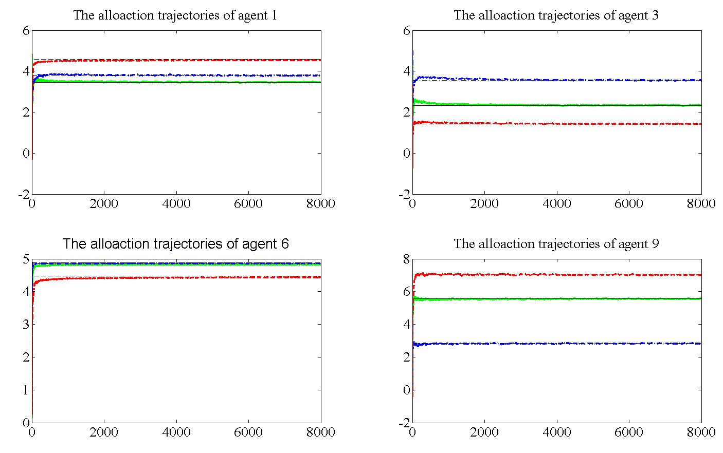
Figure 1: The averaging trajectories of some agents’ allocation variables

Consider a graph set $\mathcal{G}_{s}$ containing $30$ graphs, each of which is generated according to the random graph model $G(10,P)$, where $P$ is the probability of occurrence for any possible edge. The probability $P$ is randomly and uniformly drawn from $[0.05,0.1]$ for each graph in $\mathcal{G}_{s}$. Select a graph set $\mathcal{G}_{s}$ with its union graph being connected. At time $k$, a graph is randomly drawn from the graph set $\mathcal{G}_{s}$ according to the uniform distribution.

For $i\in\mathcal{N}$, $[\Psi_{i}]_{ij},~{}[\theta_{i}]_{j}$ are i.i.d. random variables satisfying the Gaussian distribution $N(0,0.5)$ with zero mean and variance $0.5$. Let both the generation observation noise $\delta_{i}$ and communication noise $\zeta_{ij}$, $\epsilon_{ij}$ be i.i.d. random vectors satisfying the Gaussian distribution $N(\mathbf{0},I_{3})$ with zero mean vector and covariance matrix $I_{3}$. Hence, Assumptions 4 and 5 are satisfied. The stepsize $\alpha_{k}$ in (3) is set as $\alpha_{k}=\frac{1}{(k+1)^{0.6}}$.

Experiment 1: Given a randomly generated graph set $\mathcal{G}_{s}$ and a randomly generated setting for problem (29), we apply algorithm (3) to generate $200$ independent sample paths with iteration length of $8000$. Figure 1 shows the averaging trajectories of some agents’ allocation variables, and illustrates how the agents find the optimal allocation. Moreover, Figure 2 shows the averaging trajectories of some algorithm performance indexes, including the distance to optimal solution $||P^{d}-{P^{d}}^{*}||$, function value $f(P^{d})$, $||\bar{L}\Lambda||$, and $||\sum_{i\in\mathcal{N}}(P_{i}^{d}-P_{i}^{g})||$.

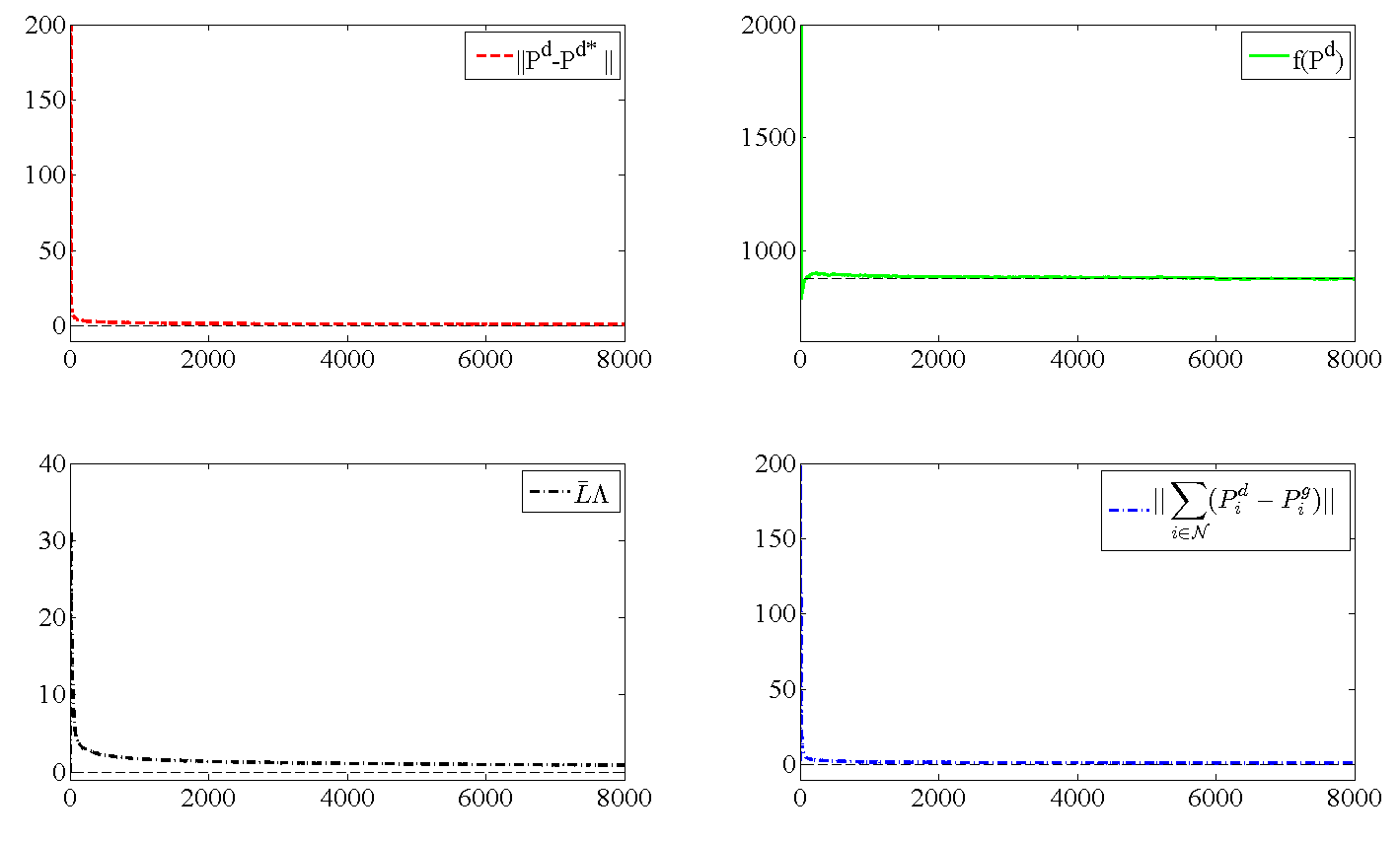
Figure 2: The averaging trajectories of some performance indexes.

Experiment 2: Let us randomly generate a graph set $\mathcal{G}_{s}$ and a setting for problem (29) at each round of this simulation, and employ algorithm (3) to generate one sample path of this setting with iteration length of $8000$. We repeat the procedure for $100$ rounds, and use Figure 3 to show the histograph of some performance indexes at iteration time $8000$. It illustrates that algorithm (3) can almost surely find the optimal allocation for different problem settings with only one sample path.

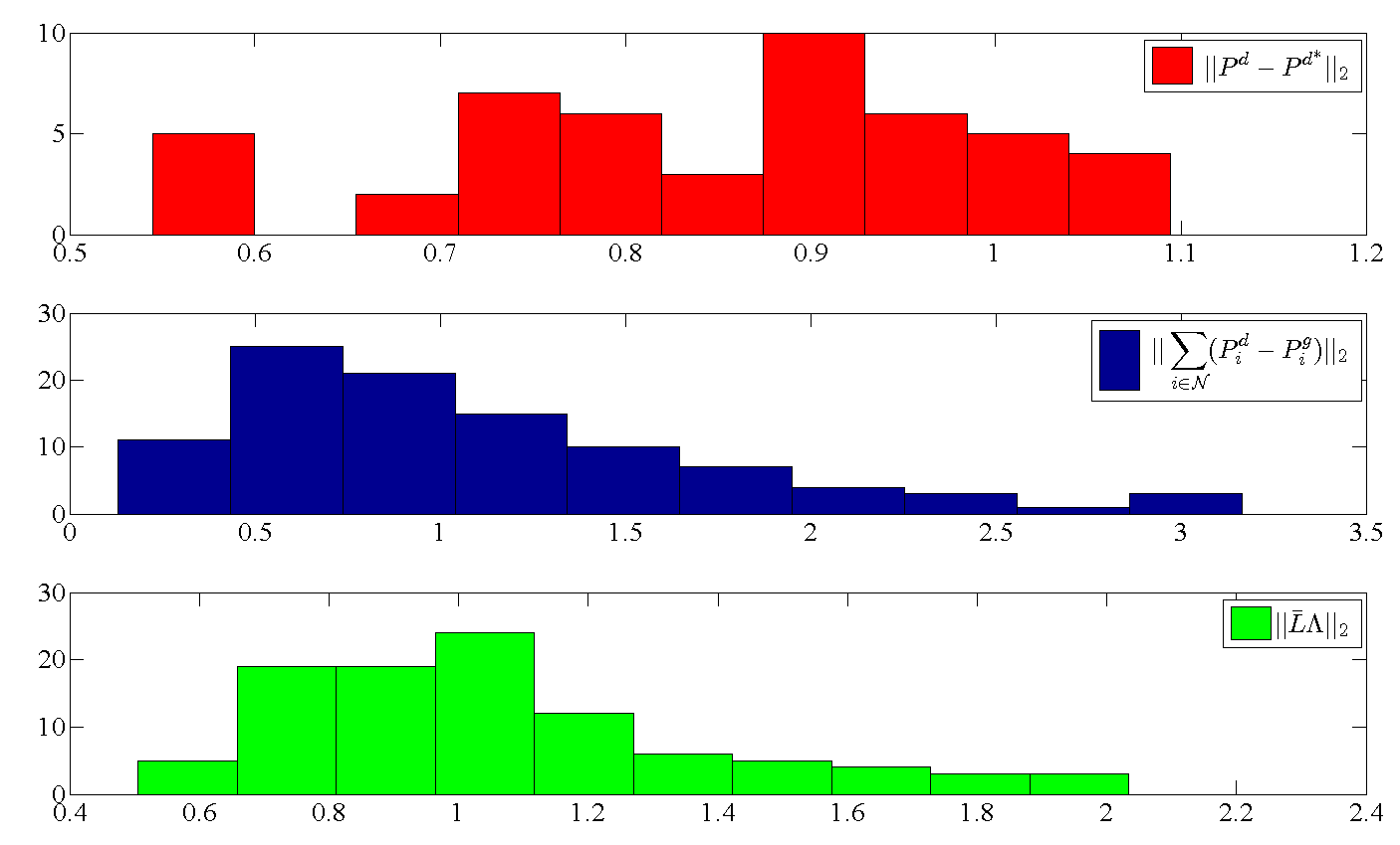
Figure 3: The histograph of some performance indexes at iteration time $k=8000$.

5 Conclusions

In this paper, an SA-based distributed algorithm was proposed to solve a class of RA optimization problems under various uncertainties. The gradient and resource observation noises were taken into consideration, and the communication network was assumed with randomly switching topologies and noisy communication channels. The algorithm was proved to converge to the optimal solution with probability one by resorting to the ODE method for SA algorithm, which may demonstrate great potentials of SA algorithm and ODE methods for distributed decision problems over network systems under noisy data observations.

Appendix

Here is the convergence result for the constrained stochastic approximation. Consider

$$\theta_{k+1}=P_{\Phi}\{\theta_{k}+\alpha_{k}Y_{k}\},$$ (30)

where $\Phi\in\mathbf{R}^{m}$ is a convex constraint set. Next follows the conditions for its convergence analysis.

C1: $\sup_{k}E[\|Y_{k}\|^{2}]<\infty.$

C2: There is a measurable function $g(\cdot)$ such that

$$E_{k}[Y_{k}]=E[Y_{k}|\theta_{0},Y_{i},i<k]=g(\theta_{k}).$$

C3: $g(\cdot)$ is continuous.

C4: $\theta_{k}$ is bounded with probability one.

Theorem 5.8

[27, Theorem 5.2.1 and Theorem 5.2.3] Let C1-C4, and (4) hold for algorithm (30). If $\Phi$ satisfies the same condition as that imposed on $\Omega_{i}$ in Assumption 2, then with probability one $\theta_{k}$ converges to the invariant set of the following projected ODE in $\Phi$:

$$\dot{\theta}=g(\theta)+z,$$

where $z\in-N_{\Phi}(\theta)$ is the minimum force to keep the trajectories of the projected ODE in $\Phi.$

The following lemma shows convergence properties for nonnegative super-martingales.

Lemma 5.9 (Robbins-Siegmund)

([29]) Let $(\Omega,\mathcal{F},\mathbb{P})$ be a probability space and $\mathcal{F}_{0}\subset\mathcal{F}_{1}\subset\cdots$ be a sequence of $\sigma-$algebra of $\mathcal{F}$. Let $\{d_{k}\}$ and $\{w_{k}\}$ be nonnegative $\mathcal{F}_{k}$-measurable random variables such that

$$E[d_{k+1}|\mathcal{F}_{k}]\leq(1+\alpha_{k})d_{k}+w_{k},$$

where $\alpha_{k}\geq 0$ are deterministic scalars with $\sum_{k=1}^{\infty}\alpha_{k}<\infty$. If $\sum_{k=1}^{\infty}w_{k}<\infty$, then $\{d_{k}\}$ converges with probability one to some finite random variable.

References

• [1] A. Ferragut, F Paganini, Network resource allocation for users with multiple connections: fairness and stability, IEEE/ACM Transactions on Networking (TON), 22(2)(2014): 349-362.
• [2] A. D’Amico, L. Sanguinetti, D.P. Palomar, Convex separable problems with linear constraints in signal processing and communictions, IEEE Transaction on Signal Processing, 62(22)(2014): 6045-6058.
• [3] C. Zhao, U. Topcu, N. Li, S. Low, Design and stability of load-side primary frequency control in power systems, IEEE Transactions on Automatic Control, 59(5)(2014):1177-1189.
• [4] T. Ibaraki, N. Katoh, Resource Allocation Problems: Algorithmic Approaches, MIT Press, Cambridge, 1988.
• [5] Y. C.  Ho, L. Servi, R.  Suri, A class of center-free resource allocation algorithms, Large Scale Systems, 1(1980): 51-62.
• [6] R. Johari, J. N.  Tsitsiklis, Efficiency Loss in a Network Resource Allocation Game, Mathematics of Operations Research, 29(3)(2004): 407-435.
• [7] A.  Nedic, A.  Ozdaglar, A. P.  Parrilo, Constrained Consensus and Optimization in Multi-Agent Networks, IEEE Transactions on Automatic Control, 55(4)(2010): 922-938.
• [8] S. Ram, A. Nedic, V. V. Venugopal, Distributed stochastic subgradient projection algorithms for convex optimization, Journal of Optimization Theory and Applications, 147(3)(2010): 516-545.
• [9] I. Lobel, A. Ozdaglar, Distributed Subgradient Methods for Convex Optimization Over Random Networks, IEEE Transactions on Automatic Control, 56(6)(2011): 1291-1306.
• [10] A. Nedic, Asynchronous Broadcast-Based Convex Optimization Over a Network, IEEE Transactions on Automatic Control, 56(6)(2011): 1337-1351.
• [11] M.  Zhu and S.  Martinez, On Distributed Convex Optimization Under Inequality and Equality Constraints, IEEE Transactions on Automatic Control, 57(1)(2012): 151-164.
• [12] Y.  Lou, G.  Shi, K. H.  Johansson, Y.  Hong, Approximate Projected Consensus for Convex Intersection Computation: Convergence Analysis and Critical Error Angle, IEEE Transactions on Automatic Control, 59(7)(2014): 1722-1736.
• [13] P.  Yi, Y.  Hong, Quantized Subgradient Algorithm and Data-Rate Analysis for Distributed Optimization, IEEE Transactions on Control of Network Systems, 1(4)(2014): 380-392.
• [14] L. Xiao, S. Boyd, Optimal Scaling of a gradient method for distributed resource allocation, Journal of Optimization Theory and Applications, 129(3)(2006): 469-488.
• [15] H.  Lakshmanan, D. P.  Farias, Decentralized Resource Allocation in Dynamic Networks of Agents, SIAM J. Optim., 19(2)(2008): 911-940.
• [16] E. Ghadimi, I. Shames, M. Johansson, Multi-Step Gradient Methods for Networked Optimization, IEEE Transactions on Signal Processing, 61(21)(2013): 5417-5429.
• [17] A.  Beck, A.  Nedic, A.  Ozdaglar, M.  Teboulle, Optimal Distributed Gradient Methods for Network Resource Allocation Problems, IEEE Transactions on Control of Network Systems, 1(1)(2014): 64-74.
• [18] A. Nemirovski, A. Juditsky, G. Lan, Robust stochastic approximation approach to stochastic programming, SIAM Journal on Optimization, 19(4)(2009): 1574-1609.
• [19] J. Lei, H-F. Chen, Distributed Stochastic Approximation Algorithm With Expanding Truncations: Algorithm and Applications, arXiv: 1410.7180v2
• [20] D. Yuan, D. W. C. Ho, Randomized gradient-free method for multiagent optimization over time-varying networks, IEEE Trans. Neural Networks and Learning Systems, published online, 2014. DOI:10.1109/TNNLS.2014.2336806.
• [21] V. Cevher, S. Becker, M. Schmidt, Convex Optimization for Big Data: Scalable, randomized, and parallel algorithms for big data analytics, IEEE Signal Processing Magazine, 31(5)(2014): 32-43.
• [22] K. Srivastava, A. Nedic, D. Stipanovic, Distributed Constrained Optimization over Noisy Networks, in Proceeding of the 49th IEEE Conference on Decision and Control, Atlanta, Georgia, 2010, pp. 1945-1950.
• [23] S. Boyd, A. Ghosh, B. Prabhakar, D. Shah, Randomized gossip algorithms, IEEE Transactions on Information Theory, 52(6)(2006): 2508-2530.
• [24] Q. Zhang, J-F. Zhang, Distributed Parameter Estimation Over Unreliable Networks With Markovian Switching Topologies, IEEE Transactions on Automatic Control, 57(10)(2012): 2545-2560.
• [25] S. Han, U. Topcu, G. J. Pappas, Differentially Private Distributed Constrained Optimization, arXiv: 1411.4105, http://arxiv.org/abs/1411.4105.
• [26] H-F Chen, T. E. Duncan, B. Pasik-Duncan, A Kiefer-Wolfowitz algorithm with randomize difference, IEEE Transactions on Automatic Control, 44(3)(1999): 442-453.
• [27] H. J. Kushner, G. Yin, Stochastic approximation: recursive algorithms and applications, Springer, New York, 2003.
• [28] V. S. Borkar, Stochastic Approximation: A Dynamical Systems Viewpoint, Cambridge University Press, Cambridge, UK, 2008.
• [29] H. Robbins and D. Siegmund, A convergence theorem for non negative almost supermartingales and some applications, Optimizing Methods in Statistics, 1971:233-257.
• [30] P.  Yi, Y.  Hong, F.  Liu, Distributed Gradient Algorithm for Constrained Optimization with Application to Load Sharing in Power Systems, Systems & Control Letters, 83(2015): 43-52.