Interplay of Rashba spin orbit coupling and disorder in the conductance properties of a four terminal junction device

Abstract

We report a thorough theoretical investigation on the quantum transport of a disordered four terminal device in the presence of Rashba spin orbit coupling (RSOC) in two dimensions. Specifically we compute the behaviour of the longitudinal (charge) conductance, spin Hall conductance and spin Hall conductance fluctuation as a function of the strength of disorder and Rashba spin orbit interaction using the Landauer B${\ddot{\mathrm{u}}}$ttiker formalism via Green’s function technique. Our numerical calculations reveal that both the conductances diminish with disorder. At smaller values of the RSOC parameter, the longitudinal and spin Hall conductances increase, while both vanish in the strong RSOC limit. The spin current is more drastically affected by both disorder and RSOC than its charge counterpart. The spin Hall conductance fluctuation does not show any universality in terms of its value and it depends on both disorder as well as on the RSOC strength. Thus the spin Hall conductance fluctuation has a distinct character compared to the fluctuation in the longitudinal conductance. Further one parameter scaling theory is studied to assess the transition to a metallic regime as claimed in literature and we find no confirmation about the emergence of a metallic state induced by RSOC.

1 Introduction

Spintronics or spin based electronics focuses on transportation of electron spins in a variety of semiconducting materials wolf ; dd ; murakami . The prospects of obtaining a dissipation less spin current along with a large number of applications possible, have generated intense activities from both the theoreticians and the experimentalists.

While there were early attempts of injecting spin polarized charge carries (from ferromagnetic metals) in non magnetic semiconductors (thereby converting them to dilute magnetic semiconductors) which have yielded very limited success. However the recent discovery of intrinsic spin Hall effect (SHE) in p-type semiconductors, that originate from an effective magnetic field and induced by a Berry phase makes the up and down spin electrons drift in opposite directions contribute immensely to the ongoing experimental work on spin manipulation phenomena in real materials murakami . In two dimensional electron gases (2DEG), one can hope to realize some of the interesting physics in this regard in presence of Rashba spin orbit coupling (RSOC) sinora .

In this work we shall concentrate on Hall effect (for both charge and spin) induced by RSOC in a four terminal junction device in presence of disorder. The existing work on the subject of interplay of disorder and RSOC on the conductance properties of such junction devices is limited and not beyond controversy shen ; burkov ; schhemann .

In a simple language, the existence of RSOC distinguishes the up and down spin electrons and hence a potential gradient applied in the $x$-direction, the opposite spins drift towards mutually opposite $y$-direction and an accumulation of spins can be observed along the edges of the sample, thereby yielding SHE. In experiments such accumulation of spins could be optically detected by using the Kerr rotation spectroscopy kato ; sih . Now, as disorder is mostly an inextricable component in real systems, we seek to study the effect of disorder on the spin Hall conductance properties of disordered samples. The issue is particularly relevant because of a number of reasons. On one hand, there are studies that claim that SHE can be strongly suppressed by disorder effects inoue signaling onset of spin relaxation and diffusion araki , while the other school of thought says that since the spins are tightly locked with their momenta (in presence of RSOC), SHE should be resilient to a disorder potential sante . Also there are suggestions of emergence of a metallic behaviour at a certain critical disorder strength in presence of RSOC, which however vanishes (as it should be) in the vanishing of the Rashba coupling shen . Therefore the scenario warrants a more complete study to settle some of the crucial issues in these regards.

Also, the universal charge conductance fluctuation lee-stone is one of the most striking quantum transport feature in mesoscopic physics, which is nothing but the consequence of quantum interference when the inelastic diffusion length exceeds sample dimensions. It is well known that the conductance fluctuations of the order of $e^{2}/h$ are universal features of quantum transport in the low temperature limit. In particular, they are independent of both the degree of disorder and the sample size at zero temperature. Analogously, one can study the fluctuations in spin Hall conductance and it is found that, there exists a universal spin Hall conductance fluctuations, which has a finite value, independent of other system details. However, this fluctuation is a function of the spin orbit interaction strength qiao ; qiao1 . In this paper we study the variation of spin Hall conductance fluctuation as a function of the disorder strength and strength of RSOC, in order to observe the universality and independent nature of spin Hall conductance fluctuation.

Motivated by the preceding discussion, we aim to investigate in a four terminal junction device the spin Hall conductance, the usual charge conductance (referred to as the longitudinal conductance), the universal spin Hall conductance fluctuation (the root mean square value of which $\left(=0.36\left(\frac{e}{8\pi}\right)\right)$ is independent of other parameters of the Hamiltonian and is thus attributed as ‘universal’ qiao .

Further we have critically examined the onset of a metallic regime at a certain critical disorder strength for a given value of the spin orbit coupling parameters as discussed by Sheng et. al shen form the behaviour of the longitudinal conductance. Their claim is as the spin orbit coupling vanishes, the critical disorder strength too vanishes, thereby yielding an absence of a metal insulator transition in two dimensions, a result that is well known.

While we are thoughtful about the applicability of a one parameter scaling theory gang_of_4 in presence of RSOC, however went ahead assuming it is at least appreciable for a particular value of the spin orbit coupling parameter. We do not find any convincing evidence in a Rashba coupled disordered four terminal junction or at best the results do not help in arriving at unambiguous inferences about it. Our inference on the ‘possible’ absence of an emerging metallic phase is justified as the Rashba term preserves the time reversal symmetry, an essential ingredient for the current ‘echo’ associated with the quantum interference effects that give rise to weak localization. An external magnetic field would have radically modified theses arguments.

In the scaling theory, the logarithmic derivative of conductance with respect to the system size is defined by a single quantity, usually denoted by $\beta$, which depends only on the conductance itself and not individually on energy, system size and disorder. Weak localization in two dimensional systems can be best characterized by the relation gang_of_4 ,

$$\beta=\frac{d\ln{G_{L}}}{d\ln{L}}$$ (1)

where, $G_{L}$ is the charge conductance and $L$ is the length of the conductor. Therefore the scenario warrants a more complete study to settle some of the crucial issues in these regards.

We organize our paper as follows. The theoretical formalism leading to the expressions for the spin Hall and longitudinal conductances using Landauer B${\ddot{\mathrm{u}}}$ttiker formula are presented in section II. Section III includes an elaborate discussion on the results obtained for the longitudinal conductance, spin Hall conductnace and fluctuation in the spin Hall conductance that are helpful in depicting the interplay of disorder strength and RSOC parameter in details.

2 Theoretical formulation

2.1 System and the Hamiltonian

Figure 1: Cross-shaped device with four semi-infinite metallic leads. The spin-orbit coupling exists in the central region only, and the effect of the semi-infinite leads is treated exactly through the self-energy terms.

In order to observe the spin Hall effect, we choose a four-probe measuring set-up as shown in Fig.1. Here the four ideal (disorder free) semi-infinite leads are attached to the central conducting region which in our case is a square lattice with Rashba spin orbit interaction. An unpolarized charge current is allowed to pass through the longitudinal leads along lead-1 and lead-2 (see Fig.1) inducing spin Hall current in the transverse directions that is along lead-3 and lead-4. The discrete spectrum of the longitudinal region is assumed to be described within the framework of tight-binding approximation assuming only nearest-neighbor hopping. The Hamiltonian for the entire system can be represented by a sum of three terms, which are,

$$H=H_{sq}+H_{leads}+H_{coupling}$$ (2)

The first term represents the Hamiltonian for the system with a square lattice geometry with Rashba spin orbit interaction and is defined by,

$$H_{sq}=\sum\limits_{i,\sigma}\epsilon_{i}c_{i\sigma}^{\dagger}c_{i\sigma}+t\sum\limits_{\langle ij\rangle,\sigma}c_{i\sigma}^{\dagger}c_{j\sigma}+$$

$$\alpha\sum\limits_{i}\left[\left(c_{i\uparrow}^{\dagger}c_{i+\delta_{x}\downarrow}-c_{i\downarrow}^{\dagger}c_{i+\delta_{x}\uparrow}\right)\right.$$

$$\left.-i\left(c_{i\uparrow}^{\dagger}c_{i+\delta_{y}\downarrow}+c_{i\downarrow}^{\dagger}c_{i+\delta_{y}\uparrow}\right)\right]$$ (3)

Here, $\epsilon_{i}$ is the random on-site potential energy chosen from a uniform rectangular distribution ($-W$ to $W$), $c_{i}^{\dagger}$ and $c_{i}$ correspond to the creation and annihilation operators respectively, for an electron at the site $i$ of the conductor. Here $t=\frac{\hbar}{2m^{*}a_{0}^{2}}$ ($m^{*}$: effective mass and $a_{0}$: lattice constant) is the hopping integral, $\alpha$ is the Rashba coupling strength. $\delta_{x,y}$ are the unit vectors along $x,y$ direction.

The four metallic leads attached to the conductor are considered to be semi-infinite and ideal. The leads are described by a similar non-interacting single particle Hamiltonian as written below,

$$H_{leads}=\sum\limits_{i=1}^{4}H_{i},$$ (4)

where

$$H_{i}=\epsilon_{L}\sum\limits_{n}c_{n}^{\dagger}c_{n}+t_{L}\sum\limits_{\langle mn\rangle}c_{m}^{\dagger}c_{n}$$ (5)

Similarly, the conductor-to-lead coupling is described by the following Hamiltonian.

$$H_{coupling}=\sum\limits_{i=1}^{4}H_{coupling,i}\quad,$$ (6)

where

$$H_{coupling,i}=t_{C}\left[c_{i}^{\dagger}c_{m}+c_{m}^{\dagger}c_{i}\right]$$ (7)

In the above expression, $\epsilon_{L}$ and $t_{L}$ stand for the site energy and nearest-neighbor hopping between the sites of the leads. The coupling between the conductor and the leads is defined by the hopping integral $t_{C}$. In Eq. 7, $i$ and $m$ belong to the boundary sites of the square lattice and leads, respectively. The summation over $i$ accounts for the four attached leads.

2.2 Formulation of longitudinal and spin Hall conductances

For the four-probe case, where pure spin current is expected to flow through the transverse leads, due to the flow of charge current through the longitudinal leads, the longitudinal and spin Hall conductances are defined as mou ,

$$G_{L}=\frac{I_{2}^{q}}{V_{1}-V_{2}}$$ (8)

and,

$$G_{SH}=\frac{\hbar}{2e}\frac{I_{3}^{s}}{V_{1}-V_{3}}=\frac{\hbar}{2e}\frac{I_{3}^{\uparrow}-I_{3}^{\downarrow}}{V_{1}-V_{3}}$$ (9)

where $I_{2}^{q}$ and $I_{3}^{s}$ are the charge and spin current flowing through the lead-2 and lead-3 respectively. $V_{m}$ is the potential at the $m$-th lead. $I_{3}^{\uparrow}$ and $I_{3}^{\downarrow}$ are the up and down spin currents flowing in lead-3.

The calculation of electric and spin currents is based on the Landauer-B${\ddot{\mathrm{u}}}$ttiker multi-probe formalism Buttiker . The charge and spin currents flowing through the lead $m$ with potential $V_{m}$, can be written in terms of spin resolved transmission probability as pareek

$$I_{m}^{q}=\frac{e^{2}}{h}\sum\limits_{n\neq m,\sigma,\sigma^{\prime}}\left(T_{nm}^{\sigma\sigma^{\prime}}V_{m}-T_{mn}^{\sigma^{\prime}\sigma}V_{n}\right)$$ (10)

$$I_{m}^{s}=\frac{e^{2}}{h}\sum\limits_{n\neq m,\sigma^{\prime}}\left[\left(T_{nm}^{\sigma^{\prime}\sigma}-T_{nm}^{\sigma^{\prime}-\sigma}\right)V_{m}+\left(T_{mn}^{-\sigma\sigma^{\prime}}-T_{mn}^{\sigma\sigma^{\prime}}\right)V_{n}\right]$$ (11)

The spin current through lead $m$ can be written in a more compact form, such as,

$$I_{m}^{s}=\frac{e^{2}}{h}\sum\limits_{n\neq m}\left[T_{nm}^{out}V_{m}-T_{mn}^{in}V_{n}\right]$$ (12)

where, we have defined two useful quantities as follows,

$$T_{pq}^{in} = T_{pq}^{\uparrow\uparrow}+T_{pq}^{\uparrow\downarrow}-T_{pq}^{\downarrow\uparrow}-T_{pq}^{\downarrow\downarrow}$$ (13)

$$T_{pq}^{out} = T_{pq}^{\uparrow\uparrow}+T_{pq}^{\downarrow\uparrow}-T_{pq}^{\uparrow\downarrow}-T_{pq}^{\downarrow\downarrow}$$ (14)

Physically, the term $\frac{e^{2}}{h}\sum\limits_{n\neq m}T_{nm}^{out}V_{m}$ in Eq. 12 is the total spin current flowing from the $m$-th lead with potential $V_{m}$ to all other $n$ leads, while the term $\frac{e^{2}}{h}\sum\limits_{n\neq m}T_{mn}^{in}V_{n}$ is the total spin current flowing into the $m$-th lead from all other $n$ leads having potential $V_{n}$.

The zero temperature conductance, $G_{pq}^{\sigma\sigma^{\prime}}$ that describes the spin resolved transport measurements, is related to the spin resolved transmission coefficient as land_cond ; land_cond2 ,

$$G_{pq}^{\sigma\sigma^{\prime}}=\frac{e^{2}}{h}T_{pq}^{\sigma\sigma^{\prime}}(E)$$ (15)

The transmission coefficient can be calculated as caroli ; Fisher-Lee ,

$$T_{pq}^{\sigma\sigma^{\prime}}=\rm{Tr}\left[\Gamma_{p}^{\sigma}G_{R}\Gamma_{q}^{\sigma^{\prime}}G_{A}\right]$$ (16)

$\Gamma_{p}^{\sigma}$’s are the coupling matrices representing the coupling between the central region and the leads, and they are defined by the relation dutta ,

$$\Gamma_{p}^{\sigma}=i\left[\Sigma_{p}^{\sigma}-(\Sigma_{p}^{\sigma})^{\dagger}\right]$$ (17)

Here $\Sigma_{p}^{\sigma}$ is the retarded self-energy associated with the lead $p$. The self-energy contribution is computed by modeling each terminal as a semi-infinite perfect wire nico .

The retarded Green’s function, $G_{R}$ is computed as

$$G_{R}=\left(E-H-\sum\limits_{p=1}^{4}\Sigma_{p}\right)^{-1}$$ (18)

where $E$ is the electron energy and $H$ is the model Hamiltonian for the central conducting region. The advanced Green’s function is, $G_{A}=G_{R}^{\dagger}$.

Now, following the spin Hall phenomenology, in our set-up since the transverse leads are voltage probes, the net charge currents through lead-3 and lead-4 is zero that is, $I_{3}^{q}=I_{4}^{q}=0$. On the other hand, as the currents in various leads depend only on voltage differences among them, we can set one of the voltages to zero without any loss of generality. Here we set $V_{2}=0$. Finally, if we assume that the leads are connected to a geometrically symmetric ordered bridge, so, $\frac{V_{3}}{V_{1}}=\frac{V_{4}}{V_{1}}=\frac{1}{2}$. Now from Eq.(12) and Eq.(9) we can write the expression of spin Hall conductance as,

$$G_{SH}=\frac{e}{8\pi}\left(T_{13}^{out}+T_{43}^{out}+T_{23}^{out}-T_{34}^{in}-T_{31}^{in}\right)$$ (19)

Similarly, from Eq. 8 and Eq. 10, the expression of longitudinal conductance can be written as,

$$G_{L}=\frac{e^{2}}{h}\left(T_{21}+\frac{1}{2}T_{32}+\frac{1}{2}T_{42}\right)$$ (20)

We define the spin Hall conductance fluctuation as,

$$\Delta G_{SH}=\sqrt{\langle G_{SH}^{2}\rangle-\langle G_{SH}\rangle^{2}}$$ (21)

where $\langle...\rangle$ denotes averaging over an ensemble of samples with different configurations with disorder strength $W$.

3 Results and discussion

We have investigated the interplay of disorder $(W)$ and ROSC $(\alpha)$ on experimentally measurable quantities such as longitudinal conductance ($G_{L}$), spin Hall conductance ($G_{SH}$) and spin Hall conductance fluctuation ($\Delta G_{SH}$). The results are likely to be relevant for systems with spin orbit interactions and since disorder is an indispensable ingredient in crystal lattices, a competition between $W$ and $\alpha$ will reveal whether they help or hinder each other with regard to the conductance properties of junction devices. An important question in this regard is whether there is any shift in the localization phenomenon in two dimensions induced by the RSOC shen . More concretely, is there a transition to a metallic state at some critical value of the strength of RSOC?

Before we start computing the physical quantities, we briefly describe the values of different parameters used in our calculation. Throughout our work, we have considered lattice constant, $a=1$, onsite term, $\epsilon=\epsilon_{L}=0$, hopping term, $t=t_{L}=t_{C}=1$. All the energies are measured in unit of $t$. Further we choose a unit where $c=h=e=1$. The longitudinal conductance, $G_{L}$ is measured in unit of $\frac{e^{2}}{h}$. The spin Hall conductance, $G_{SH}$ is measured in unit of $\frac{e}{8\pi}$. The random onsite disorder is modeled by a rectangular distribution of the form,

$$P\left(\epsilon_{i}\right)=\frac{1}{2W}\quad\rm{where,}\quad-W\leq\epsilon_{i}\leq W$$ (22)

All the results obtained below are averaged over 10000 disorder configurations.

To remind ourselves we have compared all of the above quantities at a fixed value of energy (or the biasing voltage), namely $E=-2t$. Any other energy value would yield qualitatively similar results, excepting at $E=0$ where $G_{SH}$ identically vanishes moca ; li_hu .

There is another small point that deserves a mention. We have investigated $G_{L}$, $G_{SH}$ and $\Delta G_{SH}$ both over a small range of the RSOC, that is with $[0:1]$ and also over a much broader range, namely up to $\alpha=8$. Of course, the former is a subset of the latter, but the behaviour of the physical quantities under consideration show qualitatively different behaviour in the two regimes and thus warrant distinct discussion.

3.1 Longitudinal conductance

In a tight binding model for a two dimensional square lattice, the energy band width ($BW$) is $8$ ($-4$ to $4$ in units of $t$). Here, we set range for the disorder strength, as in the interval $\left[0,\frac{BW}{2}\right]$ that is $[0,4]$, while for the RSOC strength, $\alpha$ to be in $\left[0,BW\right]$ or $\left[0,8\right]$.

The variation of $G_{L}$ as a function of $W$ for different $\alpha$ is shown in Fig.2. In this figure we have considered for $\alpha=$ 0.1, 0.3 and 1.0. As expected, $G_{L}$ falls off with disorder. However the fall off at lower values of $\alpha$ (e.g. $\alpha$ = 0.1 and 0.3) at large disorder is more than the corresponding values at large $\alpha$ (e.g. $\alpha=1$). The trend was reverse at lower values of disorder where there is a crossover at $W\approx 1.5$. For example, $G_{L}=2.5$ (in units of $\frac{e^{2}}{h}$) at $W\approx\frac{BW}{2}(=4)$ for $\alpha=1$ while the corresponding value is $\approx 1.2$ for $\alpha=0.1$.

The inference that can be drawn is larger RSOC aides in enhancing the conductance values at larger disorder. However whether this enhancement has anything got to do with a transition to a conducting phase is yet to be seen.

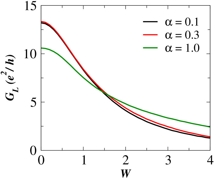
Figure 2: (Colour online) The longitudinal conductance, $G_{L}$ ( in units of $e^{2}/h$) is plotted as a function of disorder strength $W$ (in units of $t$) for different RSOC strengths, $\alpha$. Here we consider lower values of $\alpha$, namely $\alpha$ in the region $[0:1]$. The plots cross at $W\approx 1.5$. All data in this figure and all subsequent figures averaged over 10000 disorder configuration.

The variation of $G_{L}$ as a function of RSOC strength, $\alpha$ for different disorder strengths are shown in Fig.3. In Fig.3(a), $\alpha$ is varied over a small range $[0:1]$. We observe that in this regime, $G_{L}$ is not strongly dependent on $\alpha$ for the values of disorder that we have considered, namely $W=$ 1 and 4. The disorder free case is included for comparison.

However Fig.3(b) shows $G_{L}$ being plotted for a much wider rage of $\alpha$, namely $\alpha=$ 0 to $BW(=8)$. In this figure, the longitudinal conductance decreases with increasing $\alpha$ and at higher values of $\alpha$, $G_{L}$ becomes vanishingly small. Thus in this regime $\alpha$ destroys longitudinal conductance just as the disorder does. Physically, this means that large values of $\alpha$ denote strong correlated hopping anisotropies, where the hopping strengths are all different along $\pm x$ and $\pm y$ directions (see Eq.(3)). This emulates disorder effects for the charge carriers where they see a different environment with regard to hopping.

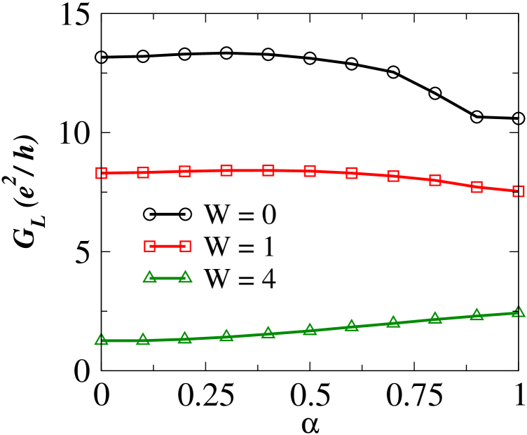
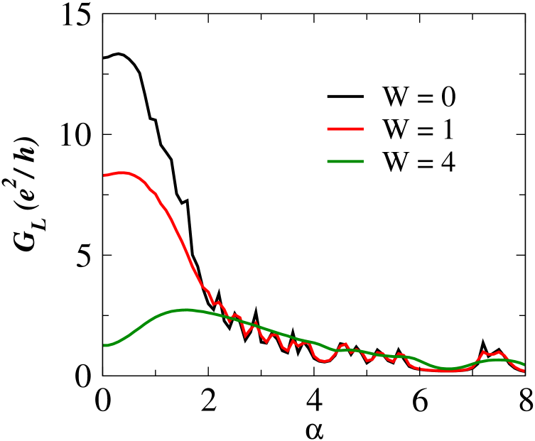
Figure 3: (Colour online) (a) $G_{L}$ is plotted as a function of RSOC strength $\alpha$ (in units of $t$) for different disorder strengths $(W)$. Here $\alpha$ is varied between $[0:1]$. $G_{L}$ has weak dependence at lower values of $\alpha$. (b) $G_{L}$ is plotted as a function of RSOC strength $\alpha$ for different disorder strengths $(W)$. Here we take the range of $\alpha$ as $[0:BW]$ $(BW=8)$. $G_{L}$ decreases with increasing the strength of RSOC.

3.2 Spin Hall conductance

We study the spin Hall conductance, $G_{SH}$ as defined by Eq.(9) in presence of disorder, $W$ and spin orbit coupling, $\alpha$. Fig. 4 shows the variation of $G_{SH}$ as a function of disorder strength, $W$ for different values of $\alpha$. Overall, $G_{SH}$ decreases with increasing disorder strength. For $\alpha=$ 0.1 and 0.3, $G_{SH}$ starts from positive values and subsequently vanishes as we increase $W$. While for $\alpha=1.0$, $G_{SH}$ starts from a negative value and vanishes at large $W$. There is a difference with the corresponding data for the longitudinal conductance, $G_{L}$ which remains finite at large disorder.

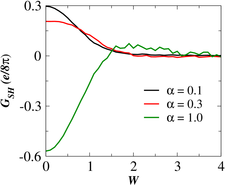
Figure 4: (Colour online) The spin Hall conductance, $G_{SH}$ (in units of $e/8\pi$) is plotted as a function of disorder strength, $W$ for different RSOC strengths, $\alpha$. $G_{SH}$ decreases with increasing the disorder strength, $W$.

Fig.5 shows the variation of $G_{SH}$ as a function of $\alpha$ for different values of $W$. In Fig.5(a), we have plotted $G_{SH}$ for a small range of $\alpha$, namely between $[0:1]$. As expected, for the pure case ($W=0$), $G_{SH}$ has a maximum value (in magnitude). As disorder is introduced, the spin Hall conductance decreases. In Fig.5(b), $G_{SH}$ is plotted for a wider range of $\alpha$. It is in tune with the results for longitudinal conductance that at higher values of $\alpha$, $G_{SH}$ becomes almost zero. However $G_{SH}$ seem to be strongly affected by disorder. At $W=4$, for all values of $\alpha$, $G_{SH}\approx 0$. There is a fluctuation in $G_{SH}$, the behaviour of which may be due to the finite size effects moca .

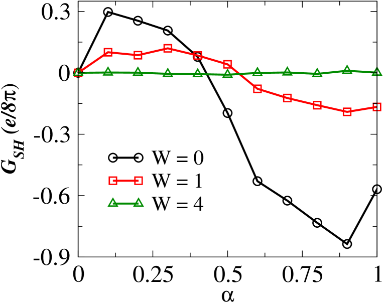
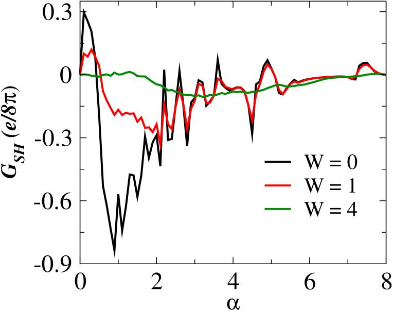
Figure 5: (Colour online) Spin Hall conductance, $G_{SH}$ is plotted as a function of RSOC strength $\alpha$ for $W=$ 0, 1 and 4. (a) $\alpha$ is varying from $[0:1]$. (b) $\alpha$ is varying for a much wider range, that is between $[0:8]$.

3.3 Spin Hall conductance fluctuation

As said earlier, the spin Hall conductance fluctuation attains a finite constant value which is independent of material properties. It is thus of importance to see how this otherwise constant value responds to disorder and RSOC.

In Fig. 6(a), $\Delta G_{SH}$ (in unit of $\frac{e}{8\pi}$) is plotted as a function of $W$ for different values of $\alpha$. As we increase $\alpha$ the fluctuation also increases. For each value of $\alpha$ and at lower values of $W$, it may be noted that, $\Delta G_{SH}$ increases linearly, and hence it reaches a maximum value. Beyond this, $\Delta G_{SH}$ decreases with increasing $W$, yielding a non-monotonic behaviour qiao .

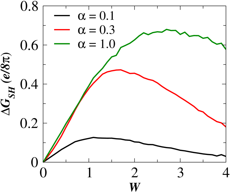
Figure 6: (Colour online) (a) $\Delta G_{SH}$ (in units of $e/8\pi$) is plotted as a function of disorder strength $W$ for different RSOC strengths $(\alpha)$. $\Delta G_{SH}$ shows a non monotonic behaviour with disorder, $W$.

Fig.7 shows the variation of $\Delta G_{SH}$ as a function of $\alpha$ for different values of the disorder strength. In Fig.7(a), for small disorder values, that is $W=0.5$ and $1$, $\Delta G_{SH}$ tends to saturate at values, namely 0.2 and 0.4 respectively. As we increase disorder, the fluctuation also increases and the corresponding plot shows no saturation upto $W=4$. In Fig.7(b), we have shown the variation of $\Delta G_{SH}$ for a wider range of $\alpha$, which shows a non-monotonic behaviour, beyond $\alpha\approx 1$ and ultimately vanishing at large values of $\alpha$, albeit not without fluctuation. Further the plots for lower values of disorder (e.g. $W=$ 0.5 and 1, as compared to $W=1$) show suppressed fluctuations.

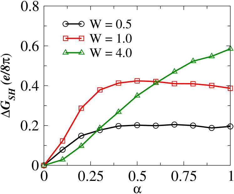
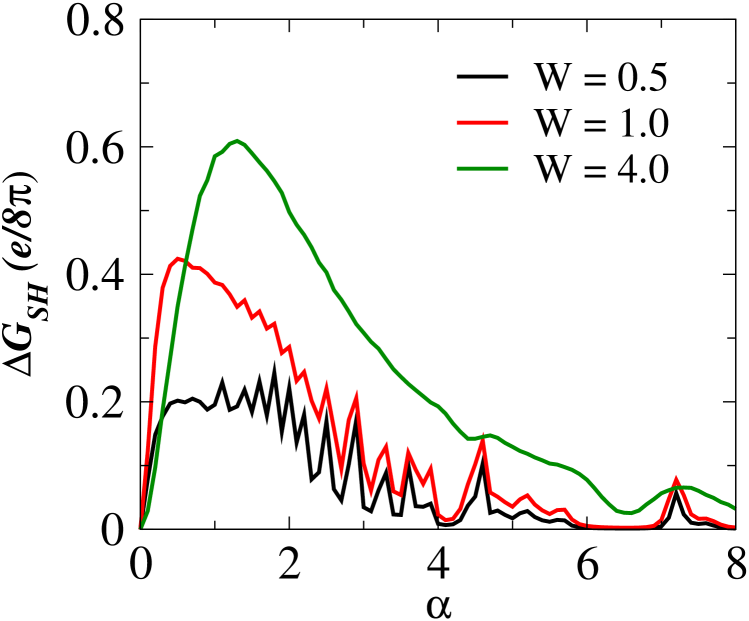
Figure 7: (Colour online) (a) $\Delta G_{SH}$ is plotted as a function of RSOC strength $\alpha$ for $W=$ 0.5, 1 and 4 for a small range of $\alpha$, that is between $[0:1]$. (b) $\Delta G_{SH}$ is plotted as a function of RSOC strength $\alpha$ for a much wider range, namely between $[0:8]$.

It may be noted that in the fluctuation in spin Hall conductance we did not find any universality in presence of disorder and RSOC. $\Delta G_{SH}$ depends on the disorder strength, $W$ and the strength of the RSOC, $\alpha$.

3.4 One parameter scaling theory

It may be noted that the following observations were made in Fig.3, that the longitudinal conductance, $G_{L}$ is seen to increase at larger disorder $\left(W\sim\frac{B}{2}\right)$ as $\alpha$ increases. At $\alpha=1$, $G_{L}$ is greater than that corresponding to other lower values of $\alpha$. This enhancement in conductance whether signals a transition to a metallic phase as hinted in Ref.shen is to be assessed. To arrive at a conclusion we perform a one parameter scaling theory gang_of_4 . For that, we study the variation of $\beta$ as a function of $1/G_{L}$ in presence of RSOC and random onsite disorder. The results are shown in Fig.8. In Fig. 8(a), $\beta$ is plotted as a function of $1/G_{L}$ for two disorder strengths, namely $W=$ 1 and 3, where we have kept $\alpha$ to be constant at a very low value, such as 0.05. In Fig. 8(b), we take a larger value of $\alpha(=1.0)$. In both Fig.8, the maximum values of $\beta$ attain values close to zero, however there is no crossing of the dashed line $(\beta=0)$ in Fig.8. $\beta$ becoming positive (convincingly staying above the dashed line) would have indicated a transition to a metallic phase as the conductance directly scaling with system size is a typical signature for the presence of extends states and hence metallic behaviour. Hence we can not say anything about the existence of onset of a metallic regime at a certain critical disorder strength for a given value of the spin orbit coupling parameters as informed by Sheng et. al. shen .

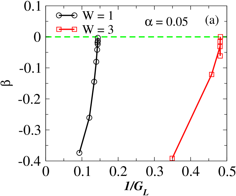
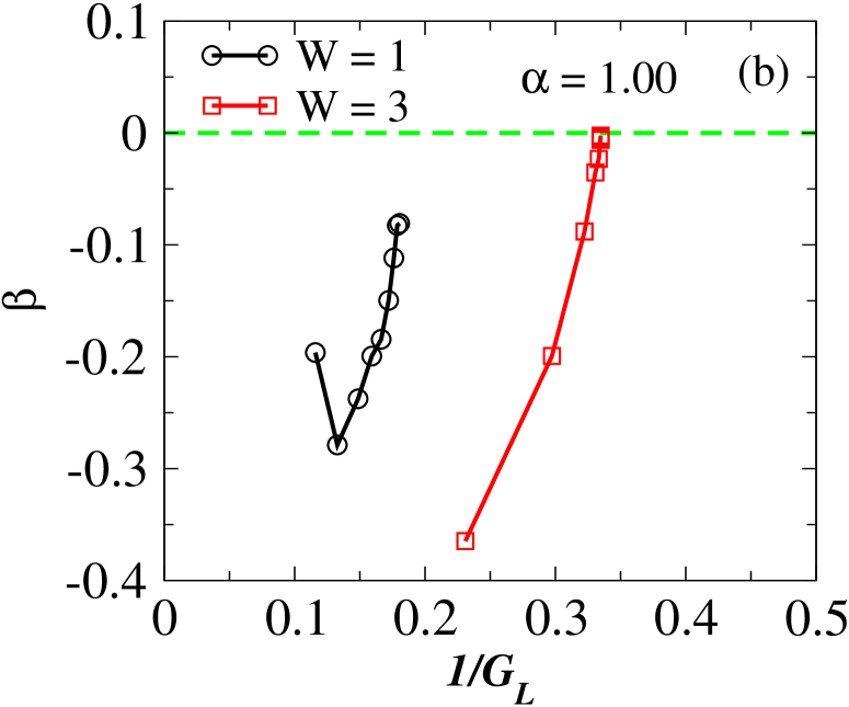
Figure 8: (Colour online) $\beta$ is plotted as a function of $1/G_{L}$. (a) $\alpha=0.05$ , (b) $\alpha=1.0$. In both the figures, the strengths of disorder, $W$ are 1 and 3. The plots do not cross the dashed line $(\beta=0)$ and always remain negative.

4 Summary and Conclusion

In summary, in the present work we have studied the interplay of random onsite disorder, $W$ and the strength of RSOC, $\alpha$ on the conductance properties of a four-probe junction device. Both these factors destroy the longitudinal $(G_{L})$ and spin Hall conductances $(G_{SH})$ for the parameter regime that we have considered in our work, namely $0\leq W\leq\frac{BW}{2}$ and $0\leq\alpha\leq BW$ ($BW$: bandwidth = 8$t$). For lower values of $\alpha$ ($0\leq\alpha\leq 1$), $G_{L}$ shows weak dependence on $\alpha$ and vanishes at large values of $\alpha$. Further, $G_{L}$ diminishes as disorder is increased: larger $\alpha$ registes a higher conductance at strong disorder ($W=4$).

The spin Hall conductance, $G_{SH}$ is more strongly affected by disorder (than $G_{L}$) which vanishes at $W\approx 1.5$ and again a larger $\alpha$ yields larger conductance at low disorder. Further $G_{SH}$ shows an antisymmetric behaviour for $0\leq\alpha\leq 1$, while it vanishes at larger $\alpha$, albeit with some fluctuations. These fluctuations remain even after the configuration averaging being done over 10000 disorder realizations.

Further the spin Hall conductance fluctuations, $\Delta G_{SH}$ do not have a universal nature and shows strong dependencies on $W$ and $\alpha$, all the while remaining at lower than its universal value $\frac{e}{8\pi}$.

Finally we do not get any convincing evidence for a RSOC induced transition to a metallic state and we feel that it is a physically meaningful result as the RSOC does not break the time reversal symmetry, a crucial condition for the weak localization to occur, which however could have been a different scenario if an external magnetic field would have been present.

5 Acknowledgment

For most of our numerical calculations we have used KWANT kwant . SB thanks CSIR India for financial support under the Grant F.No:03(1213)/12/EMR-II.

6 References

References

- (1) S. A. Wolf, D. D. Awschalom, R. A. Buhrman, J. M. Daughton, S. von Molnr, M. L. Roukes, A. Y. Chtchelkanova and D. M. Treger, Science 294, 1488 (2001).
- (2) D.D. Awschalom, D. Loss, N. Samarth, Semiconductor Spintronics and Quantum Computation, Springer 2002.
- (3) S. Murakami, N. Nagaosa, S-C Zhang, Science 301, 5638 (2003).
- (4) J. Sinova, D. Culcer, Q. Niu, N. A. Sinitsyn, T. Jungwirth and A. H. MacDonald, Phys. Rev. Lett. 92, 126603 (2004).
- (5) L. Sheng, D. N. Sheng and C. S. Ting, Phys. Rev. Lett. 94, 016602 (2005).
- (6) A. A. Burkov, A. S. Nuz and A.H. MacDonald, Phys. Rev. B 70, 155308 (2004).
- (7) J. Schliemann and D. Loss, Phys. Rev. B 69, 165315 (2004).
- (8) Y. K. Kato, R. C. Myers, A. C. Gossard and D. D. Awschalom, Science 306, 1910 (2004).
- (9) V. Sih, R. C. Myers, Y. K. Kato, W. H. Lau, A. C. Gossard and D. D. Awschalom, Nature Physics 1, 31 (2005).
- (10) Jun-ichiro Inoue, Gerrit E. W. Bauer, and Laurens W. Molenkamp, Phys. Rev. B 70, 041303(R) (2004).
- (11) Y. Araki, G. Khalsa, and A. H. MacDonald, Phys. Rev. B 90, 125309 (2014).
- (12) D. D. Sante, P. Barone, E. Plekhanov, S. Ciuchi and S. Picozzi, Scientific Reports 5, 11285 (2015).
- (13) E. Abrahams, P. W. Anderson, D. C. Licciardello and T. V. Ramakrishnan, Phys. Rev. Lett. 42, 673 (1979).
- (14) P. A. Lee and A. D. stone, Phys. Rev. Lett. 55, 1622 (1985).
- (15) W. Ren, Z. Qiao, J. Wang, Q. Sun and H. Guo, Phys. Rev. Lett. 97, 066603 (2006).
- (16) Z. Qiao, J. Wang, Y. Wei and H. Guo, Phys. Rev. Lett. 101, 016804 (2008).
- (17) M. Dey, S. K. Maiti and S. N. Karmakar, J. Appl. Phys. 112, 024322 (2012).
- (18) M. Bttiker, Phys. Rev. Lett. 57, 1761 (1986).
- (19) T. P. Pareek, Phys. Rev. Lett. 92, 076601 (2004).
- (20) R. Landauer, IBM J. Res. Dev. 1, 223 (1957).
- (21) R. Landauer, Philos. Mag. 21, 683 (1970).
- (22) C. Caroli, R. Combescot, P. Nozieres and D. Saint-James, J. Phys C: Solid State Phys. 4, 916, (1971).
- (23) D. S. Fisher and P. A. Lee, Phys. Rev. B 23, 6851 (1981).
- (24) S. Dutta, Electronic transport in Mesoscopic systems, University press (Cambridge), (1995).
- (25) B. K. Nikolic, Phys. Rev. B 64, 014203 (2001).
- (26) C. P. Moca and D. C. Marinescu, Phys. Rev. B. 72, 165335 (2005).
- (27) J. Li, L. Hu and S. Q. Shen, Phys. Rev. B. 71, 241305(R) (2005).
- (28) C. W. Groth, M. Wimmer, A. R. Akhmerov, X. Waintal, Kwant: a software package for quantum transport, New J. Phys. 16, 063065 (2014).