Decay estimates of discretized Green’s functions for Schrödinger type operators

Abstract

For a sparse non-singular matrix $A$, generally $A^{-1}$ is a dense matrix. However, for a class of matrices, $A^{-1}$ can be a matrix with off-diagonal decay properties, i.e., $\lvert A^{-1}_{ij}\rvert$ decays fast to $0$ with respect to the increase of a properly defined distance between $i$ and $j$. Here we consider the off-diagonal decay properties of discretized Green’s functions for Schrödinger type operators. We provide decay estimates for discretized Green’s functions obtained from the finite difference discretization, and from a variant of the pseudo-spectral discretization. The asymptotic decay rate in our estimate is independent of the domain size and of the discretization parameter. We verify the decay estimate with numerical results for one-dimensional Schrödinger type operators.

65N80, 65Z05

Citation:​​​​

LIN L. and LU J. . Sci China Math, 2016, 59, doi:

1 Introduction

Consider the following Schrödinger type partial differential equation

$$\lambda G(x,y)-(-\Delta+V(x))G(x,y)=\delta(x-y),\quad x,y\in\Omega\subset\mathbb{R}^{d}.$$ (1.1)

Here $\Omega=[0,L)^{d}$ is a cubic domain with periodic boundary conditions. $V(x)$ is a real, smooth potential function. Here $\delta(x)$ is the Dirac $\delta$-distribution, and $\lambda\in\mathbb{C}$ is in the resolvent set of the Hamiltonian operator $H:=-\Delta+V(x)$. Then $G$ is called the Green’s function of $\lambda-H$. It can be shown that $G$ decays exponentially to zero along the off-diagonal direction. Roughly speaking, if the domain size $L$ is large enough, for each fixed $y\in\Omega$, the magnitude of $G(x,y)$ decays exponentially as $d(x,y)$ increases, where $d(x,y)$ is the distance between $x,y\in\Omega$ interpreted in the periodic sense. Furthermore, such decay rate is independent of the domain size $L$. In fact, the following theorem has been established in the previous work [ELu:11] by one of the authors for Hamiltonian operators defined on $\mathbb{R}^{d}$ (and hence contains the current periodic case as a special situation).

Theorem (E-Lu 2011 [ELu:11]).

Assume $\lambda$ lies in the resolvent set of $H$, then there exist constants $\gamma,C>0$ such that

$$\sup_{y\in\mathbb{R}^{d}}\left\|e^{\gamma((\cdot-y)^{2}+1)^{1/2}}(\lambda-H)^{-1}e^{-\gamma((\cdot-y)^{2}+1)^{1/2}}\right\|_{\mathcal{L}(L^{2})}\leq C,$$

where the exponential functions are viewed as multiplication operators.

The decay property is a powerful tool for designing efficient numerical methods, such as the sparse approximate inverse preconditioner (AINV) [BenziMeyerTuma1996, BenziTuma1998], incomplete $LU$ and Cholesky type factorization [Saad1994], and localized spectrum slicing [Lin2014]. It also has profound implication in science and engineering applications. In quantum physics literature, the exponential decay property of Green’s functions and related physical quantities is referred to as the “near-sightedness principle” [Kohn1996, ProdanKohn2005] of electronic matters. A variety of “linear scaling” methods for solving Kohn-Sham density functional theory [KohnSham1965] for gapped systems have been proposed in the past two decades, such as the divide-and-conquer method [Yang1991, ChenLu2014], and remains an active research field (see e.g., the review articles [Goedecker1999, BowlerMiyazaki2012, BenziBoitoRazouk2013]).

In order to develop efficient numerical methods taking advantage of the decay property of Green’s functions, we require the Schrödinger operator to be discretized using a certain numerical scheme. It turns out that not all numerical discretization schemes lead to discretized Green’s function with exponentially decaying off-diagonal elements. This paper is concerned with demonstrating that discretized Green’s functions obtained from proper numerical schemes also have decay properties, either exponentially or super-algebraically. We obtain decay estimates of which the decay rate is asymptotically independent of the discretization parameter (e.g., the grid size in finite difference discretization), and of the domain size. To the best of our knowledge, such results were not known in previous literature.

Previous work:

The exponential decay properties of Green’s functions in the continuous setup and the related exponential decay of eigenfunctions of elliptic operators have been widely studied (see e.g., [Agmon:65, CombesThomas:73, Simon:83, ELu:11, ELu:13]).

In the discretized setup, the exponential decay of discretized Green’s functions was first studied in [Demko1977, DemkoMossSmith1984] for the matrix inverse $A^{-1}$, where $A$ is assumed to be a banded, positive definite matrix. In order to generalize from banded matrices to general sparse matrices, decay properties should be defined using geodesic distances of the graph induced by $A$. These techniques have been used in [BenziBoitoRazouk2013, BenziRazouk2007] and references therein, for demonstrating the decay properties of e.g., Fermi-Dirac operators in electronic structure theory. This type of decay estimate relies on the following facts: 1) a complex analytic function such as $z^{-1}$ where $z$ belongs to a simply connected complex domain away from $0$, can be efficiently expanded using polynomials of controllably low degrees, and 2) when the matrix size is sufficiently large, a finite term polynomial of a sparse matrix remains a sparse matrix. This argument can be further generalized to non-sparse matrices with exponentially decaying off-diagonal elements, and is not restricted to Schrödinger type operators in Eq. (1.1). It can be shown that the exponent for the exponential decay estimate is bounded by a constant while increasing the domain size $L$. However, the decay rate is not uniform with respect to the refinement of the discretization parameter.

Simply speaking, the reason why the general argument above cannot produce optimal decay estimates with increasingly refined discretization is as follows. Due to the presence of the Laplacian operator $-\Delta$, $H$ is an unbounded operator. The spectral radius of the discretized $H$ increases as the discretization refines. For instance, for finite difference discretization with uniform grid spacing $\Delta x$, the spectral radius of the discretized $H$ increases as $\mathcal{O}(\Delta x^{-2})$. As a result, the order of polynomials needed to accurately approximate the complex analytic function such as $z^{-1}$ increases as $\mathcal{O}(\Delta x^{-2})$, and the decay rate deteriorates. In the limit when the $\Delta x\to 0$, it can be shown that the exponential decay rate in the “physical” space approaches $0$. However, as $\Delta x\to 0$ the discretized Green’s function should well approximate the continuous Green’s function up to consistency error, and hence should share the decay property of the continuous Green’s functions. The discrepancy between the decay properties of the discrete and continuous versions of the Green’s functions is due to the fact that such decay estimates for discretized Green’s function provides only a lower bound of the exponential decay rate, and such lower bound is not optimal. Therefore, this type of estimate is mostly suitable for discretized $H$ with relatively small spectral radius, i.e., discretization with low to medium accuracy. It is desirable to have a better estimate which correctly captures the decay behavior for all accuracy level.

Our contribution:

In this paper we provide decay estimates of discretized Green’s functions for Schödinger type operators. The decay rate of our estimates is asymptotically independent of both the domain size and the discretization parameter. We demonstrate the decay estimate for two types of discretization: finite difference discretization and a variant of the pseudo-spectral discretization. Our result is explicitly stated for one-dimensional Schrödinger type operators. However, generalization to Schrödinger type operators in higher dimensions is straightforward with necessary notational changes.

For the finite difference discretization, our argument is analogous to the decay estimate of continuous Green’s functions [ELu:11]. Compared to the general argument in e.g., [Demko1977, BenziBoitoRazouk2013] based on matrix sparsity, our method specifically exploits the structure of the discretized Laplacian operator. More specifically, we use the discretized Green’s function, which is a matrix of bounded spectral radius, to control other operators with diverging spectral radius. Such operators include the discretized first and second order differential operators. We find that the discretized Green’s function decays exponentially along the off-diagonal direction (see Theorem 2.3).

For the pseudo-spectral discretization, the off-diagonal elements of the discretized $H$ only decay polynomially. We verify numerically that the corresponding discretized Green’s function does not decay exponentially along the off-diagonal direction. However, if we systematically mollify the high end of the spectrum of the discretized Laplacian operator, the resulting discretized $H$ will decay super-algebraically along the off-diagonal direction. We refer to this scheme as the mollified pseudo-spectral method (mPS). We demonstrate that the off-diagonal elements of the discretized Green’s function corresponding to the mPS discretization decay super-algebraically. For any given polynomial order, the decay rate does not depend on the domain length or the discretization parameter (see Theorem 3.10 and Theorem 3.14). The proof of this result relies on the discrete version of the relation between the regularity of the Fourier space and the decay in the real space.

Notation:

The following notation is used throughout the paper. With some abuse of notation, unless otherwise clarified, the symbol $H$ denotes both the continuous operator $-\Delta+V(x)$, and its discretized matrix, for both the finite difference discretization and for the pseudo-spectral type discretization. Similarly $G$ denotes both the continuous Green’s function for the operator $\lambda-H$ and its discretized matrix. $\imath$ stands for the imaginary unit. The complex conjugate of a complex number $f$ is denoted by $f^{*}$. The identity matrix is denoted by $I$. When the identity matrix is multiplied by a scalar $\lambda$, the matrix $\lambda I$ is also denoted by $\lambda$ for simplicity, unless otherwise clarified.

For simplicity of the notation, we will restrict ourselves to the cases that the computational domain is an interval $\Omega=[0,L)$ in one spatial dimension. The extension to higher spatial dimensional rectangular computational domain is straightforward. The computational domain is discretized by $N$ equispaced grid points: $\mathcal{X}=\{x_{i}\mid x_{i}=i\Delta x,i=0,1,\ldots,N-1\}$, where $\Delta x=L/N$ is the grid size.

Throughout this paper, since we are only interested in the asymptotic decay behavior, we will assume that $L\geq 1$ and also without loss of generality $\Delta x\leq 1$.

For a lattice function $f:\mathcal{X}\to\mathbb{R}$, we define its $L^{2}(\mathcal{X})$ norm as

$$\left\|f\right\|_{L^{2}(\mathcal{X})}^{2}=\Delta x\sum_{x\in\mathcal{X}}\left|f(x)\right|^{2},$$ (1.2)

so that as $\Delta x\to 0$, it converges to the continuous $L^{2}$ norm on $[0,L)$. Similarly the $L^{\infty}(\mathcal{X})$ norm is defined as

$$\left\|f\right\|_{L^{\infty}(\mathcal{X})}=\max_{x\in\mathcal{X}}\left|f(x)\right|.$$ (1.3)

For simplicity of the notation, we will use $\left\|f\right\|_{2}$ and $\left\|f\right\|_{\infty}$ interchangeably with $\left\|f\right\|_{L^{2}(\mathcal{X})}$ and $\left\|f\right\|_{L^{\infty}(\mathcal{X})}$, respectively.

We will focus on periodic boundary condition, so that a function $f(x)$ defined on the finite lattice $\mathcal{X}$ can be extended to a periodic function on the infinite lattice $\Delta x\mathbb{Z}$ such that $f(x+L)=f(x),x\in\mathcal{X}$.

We will use $C$ for generic absolute constants whose value may change from line to line. Specific constants are denoted as e.g., $C_{m}$ where the subscript $m$ indicates the dependence of the constant on the parameter $m$.

Organization:

This paper is organized as follows. We estimate the decay rate for the finite difference discretization in section 2, and the decay rate for the mollified pseudo-differential discretization in section 3. Numerical results demonstrating the decay rate is provided in section 4, and we conclude in section 5.

2 Finite difference discretization

In this paper we focus on the second order finite difference discretization, and it is possible to generalize the analysis to higher order finite difference discretization schemes. We define the forward and backward difference operators for $x\in\mathcal{X}$, respectively as

$$\bigl{(}\mathcal{D}^{+}f\bigr{)}(x)=\frac{1}{\Delta x}\bigl{(}f(x+\Delta x)-f(x)\bigr{)},$$ (2.1)

$$\bigl{(}\mathcal{D}^{-}f\bigr{)}(x)=\frac{1}{\Delta x}\bigl{(}f(x)-f(x-\Delta x)\bigr{)}.$$ (2.2)

The Hamiltonian operator in the second order finite difference discretization is

$$H=\mathcal{D}^{+}\mathcal{D}^{-}+V.$$ (2.3)

Here the potential function $V(x)$ is discretized into a lattice function $V:\mathcal{X}\to\mathbb{R}$ with bounded $L^{\infty}(\mathcal{X})$ norm. With some abuse of notation, unless otherwise clarified, we use $\Delta=\mathcal{D}^{+}\mathcal{D}^{-}$ to denote the discretized Laplacian operator as well.

Since periodic boundary condition is used, the natural distance between two grid points $x,y\in\mathcal{X}$ is the periodic distance

$$\widetilde{d}_{L}(x,y)=\min\bigl{\{}\left|x-y-Lk\right|,\;k\in\mathbb{Z}\bigr{\}}.$$

As in the continuous case, we need to mollify the distance to remove singularities as

$$d_{L}(x,y):=d_{\max}-\Bigl{(}\bigl{[}d_{\max}-(\widetilde{d}_{L}(x,y)^{2}+1)^{1/2}\bigr{]}^{2}+1\Bigr{)}^{1/2},$$ (2.4)

where $d_{\max}=\max\,(\widetilde{d}_{L}(x,y)^{2}+1)^{1/2}=(L^{2}/4+1)^{1/2}$. Note that the slightly complicated looking formula is due to the necessity of mollification when $\widetilde{d}_{L}$ is either $0$ or $L/2$. Fig. 1 gives an example of the distance function $d_{L}(x,0)$ with $L=40$.

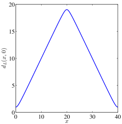
Figure 1: An illustration of the smoothed distance function $d_{L}(x,0)$ with $L=40$.

The following lemma collects the properties of $d_{L}$ that will be used for proving Theorem 2.3.

Lemma 2.1.

For fixed $y\in\mathcal{X}$, the function $d_{L}(\cdot,y)$ is twice continuous differentiable and the derivatives are bounded uniformly in $L$ and $\Delta x$.

Proof 2.2.

We include the elementary proof here for completeness. We fix $y=0$ without loss of generality, and have

$$d_{L}(x,0) =d_{\max}-\Bigl{(}\bigl{[}d_{\max}-\bigl{(}\min(\left|x\right|,\left|x-L\right|)^{2}+1\bigr{)}^{1/2}\bigr{]}^{2}+1\Bigr{)}^{1/2}$$

$$=\begin{cases}d_{\max}-\Bigl{(}\bigl{[}d_{\max}-\bigl{(}x^{2}+1\bigr{)}^{1/2}\bigr{]}^{2}+1\Bigr{)}^{1/2},&x\in[0,L/2),\\ d_{\max}-\Bigl{(}\bigl{[}d_{\max}-\bigl{(}(L-x)^{2}+1\bigr{)}^{1/2}\bigr{]}^{2}+1\Bigr{)}^{1/2},&x\in[L/2,L).\end{cases}$$

We calculate the derivative of $d_{L}(x,0)$ in each interval as follows

$$\frac{\partial d_{L}(x,0)}{\partial x}=\begin{cases}\dfrac{x\Bigl{(}d_{\max}-\bigl{(}x^{2}+1\bigr{)}^{1/2}\Bigr{)}}{\bigl{(}x^{2}+1\bigr{)}^{1/2}\Bigl{(}\bigl{[}d_{\max}-\bigl{(}x^{2}+1\bigr{)}^{1/2}\bigr{]}^{2}+1\Bigr{)}^{1/2}},&x\in[0,L/2),\\ \dfrac{-(L-x)\Bigl{(}d_{\max}-\bigl{(}(L-x)^{2}+1\bigr{)}^{1/2}\Bigr{)}}{\bigl{(}(L-x)^{2}+1\bigr{)}^{1/2}\Bigl{(}\bigl{[}d_{\max}-\bigl{(}(L-x)^{2}+1\bigr{)}^{1/2}\bigr{]}^{2}+1\Bigr{)}^{1/2}},&x\in[L/2,L).\end{cases}$$

In particular, it is continuous at $x=L/2$ and $x=0$ (viewed as a periodic function on $[0,L)$). The expression also verifies that

$$\biggl{\lvert}\frac{\partial d_{L}(x,0)}{\partial x}\biggr{\rvert}\leq 1.$$

To calculate the second order derivative, denote $\phi(t)=t/(t^{2}+1)^{1/2}$ and we write

$$\frac{\partial d_{L}(x,0)}{\partial x}=\begin{cases}\phi(x)\phi\Bigl{(}d_{\max}-\bigl{(}x^{2}+1\bigr{)}^{1/2}\Bigr{)},&x\in[0,L/2),\\ -\phi(L-x)\phi\Bigl{(}d_{\max}-\bigl{(}(L-x)^{2}+1\bigr{)}^{1/2}\Bigr{)},&x\in[L/2,L).\end{cases}$$

Hence,

$$\frac{\partial^{2}d_{L}(x,0)}{\partial x^{2}}=\begin{cases}\begin{split}&\phi^{\prime}(x)\phi\Bigl{(}d_{\max}-\bigl{(}x^{2}+1\bigr{)}^{1/2}\Bigr{)}\\ &\qquad-\phi^{2}(x)\phi^{\prime}\Bigl{(}d_{\max}-\bigl{(}x^{2}+1\bigr{)}^{1/2}\Bigr{)},\end{split}&x\in[0,L/2),\\ \begin{split}&\phi^{\prime}(L-x)\phi\Bigl{(}d_{\max}-\bigl{(}(L-x)^{2}+1\bigr{)}^{1/2}\Bigr{)}\\ &\qquad-\phi^{2}(L-x)\phi^{\prime}\Bigl{(}d_{\max}-\bigl{(}(L-x)^{2}+1\bigr{)}^{1/2}\Bigr{)},\end{split}&x\in[L/2,L).\end{cases}$$

Since $\phi^{\prime}(t)=(t^{2}+1)^{-3/2}$, it is clear that the second order derivative is uniformly bounded. To check the continuity, it suffices to check $x=L/2$ and $x=0$. We have

$$\lim_{x\to 0+}\frac{\partial^{2}d_{L}(x,0)}{\partial x^{2}}=\phi^{\prime}(0)\phi(d_{\max}-1)=\lim_{x\to L-}\frac{\partial^{2}d_{L}(x,0)}{\partial x^{2}},$$

$$\lim_{x\to L/2-}\frac{\partial^{2}d_{L}(x,0)}{\partial x^{2}}=-\phi^{2}(L/2)\phi(0)=\lim_{x\to L/2+}\frac{\partial^{2}d_{L}(x,0)}{\partial x^{2}},$$

where the second line uses that $d_{\max}=(L^{2}/4+1)^{1/2}=\lim_{x\to L/2}(x^{2}+1)^{1/2}$.

In order to prove Theorem 2.3, we need the discrete version of the Leibniz rule in the finite difference discretization. For any $x\in\mathcal{X}$,

$$\begin{split}\mathcal{D}^{-}(fg)(x)&=\frac{1}{\Delta x}\bigl{(}(fg)(x)-(fg)(x-\Delta x)\bigr{)}\\ &=\frac{1}{\Delta x}\bigl{(}f(x)-f(x-\Delta x)\bigr{)}g(x)+\frac{1}{\Delta x}f(x-\Delta x)\bigl{(}g(x)-g(x-\Delta x)\bigr{)}\\ &=\bigl{(}(\mathcal{D}^{-}f)g\bigr{)}(x)+f(x-\Delta x)\bigl{(}\mathcal{D}^{-}g\bigr{)}(x).\end{split}$$ (2.5)

Theorem 2.3.

Assume that $(\lambda-H)^{-1}$ is bounded in the matrix 2-norm, then there exist constants $\gamma_{0}>0$ and $C$ such that for any $\Delta x\leq 1$, $L\geq 1$, and $\gamma\leq\gamma_{0}$,

$$\sup_{y\in\mathcal{X}}\,\bigl{\lVert}\exp(\gamma d_{L}(\cdot,y))(\lambda-H)^{-1}\exp(-\gamma d_{L}(\cdot,y))\bigr{\rVert}_{\mathcal{L}(L^{2}(\mathcal{X}))}\leq C,$$

where $\exp(-\gamma d_{L}(\cdot,y))$ is understood as a multiplication operator:

$$\bigl{(}\exp(-\gamma d_{L}(\cdot,y))f\bigr{)}(x)=\exp(-\gamma d_{L}(x,y))f(x),\quad x\in\mathcal{X}.$$

The definition for $\exp(\gamma d_{L}(\cdot,y))$ is similar.

Proof 2.4.

Notice first that

$$\exp(\gamma d_{L}(\cdot,y))(\lambda-H)^{-1}\exp(-\gamma d_{L}(\cdot,y))=\bigl{[}\exp(\gamma d_{L}(\cdot,y))(\lambda-H)\exp(-\gamma d_{L}(\cdot,y))\bigr{]}^{-1}.$$

Using the definition of $H$, we get

$$\exp(\gamma d_{L}(\cdot,y))(\lambda-H)\exp(-\gamma d_{L}(\cdot,y)) =\exp(\gamma d_{L}(\cdot,y))(\lambda-V)\exp(-\gamma d_{L}(\cdot,y))$$

$$\qquad+\exp(\gamma d_{L}(\cdot,y))\Delta\exp(-\gamma d_{L}(\cdot,y))$$

$$=(\lambda-V)+\exp(\gamma d_{L}(\cdot,y))\Delta\exp(-\gamma d_{L}(\cdot,y))$$

Explicit calculation using (2.5) for $\mathcal{D}^{-}$ and analogously for $\mathcal{D}^{+}$, we obtain

$$\exp(\gamma d_{L}(\cdot,y))\Delta \exp(-\gamma d_{L}(\cdot,y))=\exp(\gamma d_{L}(\cdot,y))\mathcal{D}^{+}\mathcal{D}^{-}\exp(-\gamma d_{L}(\cdot,y))$$

$$=\Delta+\exp(\gamma d_{L}(\cdot,y))\bigl{[}\mathcal{D}^{-}\exp(-\gamma d_{L}(\cdot,y))\bigr{]}\mathcal{D}^{-}$$

$$\qquad+\exp(\gamma d_{L}(\cdot,y))\bigl{[}\mathcal{D}^{+}\exp(-\gamma d_{L}(\cdot,y))\bigr{]}\mathcal{D}^{+}$$

$$\qquad+\exp(\gamma d_{L}(\cdot,y))\bigl{[}\Delta\exp(-\gamma d_{L}(\cdot,y))\bigr{]}.$$

To control the lower order terms on the right hand side, we estimate

$$\Bigl{\lvert}\bigl{[}\mathcal{D}^{+}\exp(-\gamma d_{L}(\cdot,y))\bigr{]}(x)\Bigr{\rvert}=\Bigl{\lvert}\frac{1}{\Delta x}\bigl{[}e^{-\gamma d_{L}(x+\Delta x,y)}-e^{-\gamma d_{L}(x,y)}\bigr{]}\Bigr{\rvert}\\ \leq\max_{t\in[0,\Delta x]}\Bigl{\lvert}\frac{\partial}{\partial t}e^{-\gamma d_{L}(x+t,y)}\Bigr{\rvert}\leq C\max\bigl{(}\gamma e^{-\gamma d_{L}(x,y)},\gamma e^{-\gamma d_{L}(x+\Delta x,y)}\bigr{)}\leq C\gamma e^{\gamma\Delta x}e^{-\gamma d_{L}(x,y)},$$

where the first inequality follows from the mean value theorem, and the second inequality uses that $\left|\partial_{x}d_{L}(x,y)\right|$ is uniformly bounded from Lemma 2.1. The same bound also holds for $\mathcal{D}^{-}\exp(-\gamma d_{L}(\cdot,y))$. For the second order difference

$$\Bigl{\lvert}\bigl{[}\mathcal{D}^{+}\mathcal{D}^{-}\exp(-\gamma d_{L}(\cdot,y))\bigr{]}(x)\Bigr{\rvert} =\biggl{\lvert}\frac{1}{\Delta x^{2}}\bigl{[}e^{-\gamma d_{L}(x+\Delta x,y)}-2e^{-\gamma d_{L}(x,y)}+e^{-\gamma d_{L}(x-\Delta x,y)}\bigr{]}\biggr{\rvert}$$

$$=\frac{1}{\Delta x^{2}}\biggl{\lvert}\int_{0}^{\Delta x}\int_{0}^{\Delta x}\partial_{t}\partial_{s}\,e^{-\gamma d_{L}(x+(t-s),y)}\,\mathrm{d}s\,\mathrm{d}t\biggr{\rvert}$$

$$\leq\max_{(t,s)\in[0,\Delta x]^{2}}\bigl{\lvert}\partial_{t}\partial_{s}\,e^{-\gamma d_{L}(x+(t-s),y)}\bigr{\rvert}$$

$$\leq C(\gamma^{2}+2\gamma)e^{\gamma\Delta x}e^{-\gamma d_{L}(x,y)},$$

where we have used Lemma 2.1 in the last inequality.

We thus have in summary for $\gamma$ sufficiently small (recall that $\Delta x\leq 1$)

$$\left\|f^{-}\right\|_{L^{\infty}(\mathcal{X})}:=\bigl{\lVert}\exp(\gamma d_{L}(\cdot,y))\bigl{[}\mathcal{D}^{-}\exp(-\gamma d_{L}(\cdot,y))\bigr{]}\bigr{\rVert}_{L^{\infty}(\mathcal{X})}\leq C\gamma,$$

$$\left\|f^{+}\right\|_{L^{\infty}(\mathcal{X})}:=\bigl{\lVert}\exp(\gamma d_{L}(\cdot,y))\bigl{[}\mathcal{D}^{+}\exp(-\gamma d_{L}(\cdot,y))\bigr{]}\bigr{\rVert}_{L^{\infty}(\mathcal{X})}\leq C\gamma,$$

$$\left\|g\right\|_{L^{\infty}(\mathcal{X})}:=\bigl{\lVert}\exp(\gamma d_{L}(\cdot,y))\bigl{[}\Delta\exp(-\gamma d_{L}(\cdot,y))\bigr{]}\bigr{\rVert}_{L^{\infty}(\mathcal{X})}\leq C\gamma,$$

where we have introduced the short hand notation $f^{\pm}$ and $g$.

Recall the identity

$$\exp(\gamma d_{L}(\cdot,y)) (\lambda-H)\exp(-\gamma d_{L}(\cdot,y))$$ (2.6)

$$=(\lambda-V)+\Delta+\bigl{(}f^{-}\mathcal{D}^{-}+f^{+}\mathcal{D}^{+}\bigr{)}+g$$

$$=(\lambda-H)+\bigl{(}f^{-}\mathcal{D}^{-}+f^{+}\mathcal{D}^{+}\bigr{)}+g$$

$$=(\lambda-H)\biggl{[}I+\bigl{(}f^{-}\mathcal{D}^{-}+f^{+}\mathcal{D}^{+}\bigr{)}(\lambda-H)^{-1}+g(\lambda-H)^{-1}\biggr{]}.$$

Note that

$$\left\|\mathcal{D}^{-}(\lambda-H)^{-1}\right\|_{\mathcal{L}(L^{2}(\mathcal{X}))} \leq\left\|\mathcal{D}^{-}(1-\Delta)^{-1}\right\|_{\mathcal{L}(L^{2}(\mathcal{X}))}\left\|(1-\Delta)(\lambda-H)^{-1}\right\|_{\mathcal{L}(L^{2}(\mathcal{X}))}$$ (2.7)

$$\leq C\left\|(1+\lambda-V-\lambda+H)(\lambda-H)^{-1}\right\|_{\mathcal{L}(L^{2}(\mathcal{X}))}$$

$$\leq C\left(1+(\left|1+\lambda\right|+\left\|V\right\|_{L^{\infty}(\mathcal{X})})\right)\left\|(\lambda-H)^{-1}\right\|_{\mathcal{L}(L^{2}(\mathcal{X}))},$$

and the same bound for $\mathcal{D}^{+}(\lambda-H)^{-1}$. Here we have used the fact that $\left\|\mathcal{D}^{-}(1-\Delta)^{-1}\right\|_{\mathcal{L}(L^{2}(\mathcal{X}))}$ is bounded uniformly with respect to $\Delta x\leq 1$, which can be directly verified by Fourier representation. Thus by making $\gamma$ sufficiently small, the bounds on $f^{\pm}$ and $g$ guarantee the invertibility of the last term on the right hand side of (2.6) and the inverse is also bounded. The theorem is hence proved.

As a corollary to Theorem 2.3, we may infer the pointwise decay property of the Green’s function. Let us consider without loss of generality a single column $g$ of the discretized Green’s function, which solves the equation

$$(\lambda-H)g=\frac{1}{\Delta x}e_{1}$$ (2.8)

with $e_{1}=(1,0,0,\ldots,0)^{T}$. Here the prefactor $1/\Delta x$ on the right hand side of Eq. (2.8) reflects the normalization of the discrete Dirac $\delta-$distribution. Thus $g=\frac{1}{\Delta x}(\lambda-H)^{-1}e_{1}$. We estimate the exponential decay rate of $g$ (in $L^{2}$ sense) according to

$$\left\|e^{\gamma d_{L}(0,\cdot)}g\right\|_{2}=\left\|e^{\gamma d_{L}(0,\cdot)}(\lambda-H)^{-1}\frac{e_{1}}{\Delta x}\right\|_{2}=\left\|e^{\gamma d_{L}(0,\cdot)}(\lambda-H)^{-1}(1-\Delta)(1-\Delta)^{-1}\frac{e_{1}}{\Delta x}\right\|_{2}\\ \leq\left\|e^{\gamma d_{L}(0,\cdot)}(\lambda-H)^{-1}(1-\Delta)e^{-\gamma d_{L}(0,\cdot)}\right\|_{\mathcal{L}(L^{2}(\mathcal{X}))}\left\|e^{\gamma d_{L}(0,\cdot)}(1-\Delta)^{-1}\frac{e_{1}}{\Delta x}\right\|_{2}.$$ (2.9)

The right hand side of (2.9) is bounded because of the following two facts. First, similar to Eq. (2.7),

$$\left\|e^{\gamma d_{L}(0,\cdot)}(\lambda-H)^{-1}(1-\Delta)e^{-\gamma d_{L}(0,\cdot)}\right\|_{\mathcal{L}(L^{2}(\mathcal{X}))}\\ =\left\|e^{\gamma d_{L}(0,\cdot)}(\lambda-H)^{-1}(-(\lambda-H)+(\lambda+1)-V)e^{-\gamma d_{L}(0,\cdot)}\right\|_{\mathcal{L}(L^{2}(\mathcal{X}))}\\ \leq 1+\bigl{(}\left|1+\lambda\right|+\left\|V\right\|_{L^{\infty}(\mathcal{X})}\bigr{)}\left\|e^{\gamma d_{L}(0,\cdot)}(\lambda-H)^{-1}e^{-\gamma d_{L}(0,\cdot)}\right\|_{\mathcal{L}(L^{2}(\mathcal{X}))}.$$ (2.10)

Second, $\left\|e^{\gamma d_{L}(0,\cdot)}(1-\Delta)^{-1}\frac{e_{1}}{\Delta x}\right\|_{2}$ is bounded for sufficiently small $\gamma$, which can be verified by a direct calculation using the explicit discrete Green’s function for $(1-\Delta)^{-1}$ of Yukawa type. Moreover, away from $x_{1}$ (where the center of $e_{1}$ is located), local $L^{\infty}$ bounds can be obtained from the $L^{2}$ estimate combined with elliptic regularity estimates for the finite difference equation (see e.g., [ThomeeWestergren:68]). In summary, this establishes the exponential moment bound for $g$ uniform in $L$ and the discretization mesh size, thus, the Green’s function decays exponentially along the off-diagonal direction.

3 Pseudo-spectral method and mollified pseudo-spectral method

In this section we consider the pseudo-spectral type discretization. When the potential function $V$ is smooth, pseudo-spectral discretization is widely used in scientific and engineering computations. This is because pseudo-spectral type discretization gives rise to much more accurate solution than low order finite difference type discretization with the same number of degrees of freedom.

In pseudo-spectral type discretization, corresponding to the discrete lattice $\mathcal{X}$ we define the Fourier grid $\mathcal{K}=\left\{n\Delta k\mid n=-\frac{N}{2}+1,\ldots,\frac{N}{2}\right\}$. Here $\Delta k=\frac{2\pi}{L}$, the edge of the Fourier grid is defined to be

$$k_{c}:=\frac{N}{2}\Delta k=\frac{\pi N}{L}=\frac{\pi}{\Delta x}.$$ (3.1)

Note that $k_{c}\geq\pi$ due to the assumption $\Delta x\leq 1$.

For a lattice function $f:\mathcal{X}\to\mathbb{R}$, its discrete Fourier transform is defined as

$$\widehat{f}_{k}=\Delta x\sum_{x\in\mathcal{X}}e^{-\imath kx}f(x),\quad k\in\mathcal{K}.$$

The corresponding inverse discrete Fourier transform is

$$f(x)=\frac{1}{L}\sum_{k\in\mathcal{K}}e^{\imath kx}\widehat{f}_{k},\quad x\in\mathcal{X}.$$

Here the normalization factor is chosen so that when the grid spacing $\Delta x\to 0$, the discrete Fourier transform and inverse Fourier transform converges to the continuous Fourier transform and inverse Fourier transform, respectively.

Similar to Eq. (1.2) and (1.3), in Fourier space, the discrete $L^{2}(\mathcal{K})$ norm and $L^{\infty}(\mathcal{K})$ norm for $\{\widehat{f}_{k}\}$ is given as

$$\left\|\widehat{f}\right\|^{2}_{L^{2}(\mathcal{K})}=\Delta k\sum_{k\in\mathcal{K}}\left|\widehat{f}_{k}\right|^{2},\quad\left\|\widehat{f}\right\|_{L^{\infty}(\mathcal{K})}=\max_{k\in\mathcal{K}}\left|\widehat{f}_{k}\right|,$$ (3.2)

respectively. Again for simplicity of the notation, we will use $\left\|\widehat{f}\right\|_{2}$ and $\left\|\widehat{f}\right\|_{\infty}$ interchangeably with $\left\|\widehat{f}\right\|_{L^{2}(\mathcal{K})}$ and $\left\|\widehat{f}\right\|_{L^{\infty}(\mathcal{K})}$, respectively, unless otherwise clarified.

Under this choice of normalization, the discrete Parseval’s identity reads

$$\left\|\widehat{f}\right\|^{2}_{2} =\Delta k\sum_{k\in\mathcal{K}}\left|\widehat{f}_{k}\right|^{2}=\Delta k(\Delta x)^{2}\sum_{k\in\mathcal{K}}\sum_{x,x^{\prime}\in\mathcal{X}}e^{-\imath k(x-x^{\prime})}f(x)f^{\ast}(x^{\prime})$$ (3.3)

$$=\Delta kN(\Delta x)^{2}\sum_{x\in\mathcal{X}}\left|f(x)\right|^{2}=2\pi\left\|f\right\|_{2}^{2}.$$

We define the Fourier restriction operator $\mathcal{R}_{N}:L^{2}(\Omega)\to L^{2}(\mathcal{X})$ as

$$(\mathcal{R}_{N}g(\cdot))(x)=g(x),\quad x\in\mathcal{X}.$$

Similarly the Fourier interpolation operator $\mathcal{I}_{N}:L^{2}(\mathcal{X})\to L^{2}(\Omega)$ is defined as

$$[\mathcal{I}_{N}f](x)=\frac{1}{L}\sum_{k\in\mathcal{K}}\widehat{f}_{k}e^{\imath kx},\quad x\in\Omega.$$

Using the Fourier restriction and interpolation operator, the Laplacian operator in the pseudo-spectral discretization becomes $\mathcal{R}_{N}\Delta\mathcal{I}_{N}$. For simplicity we consider the case in the absence of the external potential i.e. $V(x)=0$, and $\lambda=-1$. In this case, the pseudo-spectral discretization is equivalent to the spectral discretization, and Eq. (1.1) becomes

$$(1-\mathcal{R}_{N}\Delta\mathcal{I}_{N})G=-\frac{1}{\Delta x}I.$$ (3.4)

Again the prefactor $1/\Delta x$ on the right hand side of Eq. (3.4) reflects the normalization of the discrete Dirac $\delta-$distribution. Since $\mathcal{R}_{N}\Delta\mathcal{I}_{N}$ is translational invariant, without loss of generality we only consider the first column of $G$, denoted by $g$. Then

$$(1-\mathcal{R}_{N}\Delta\mathcal{I}_{N})g=-\frac{1}{\Delta x}e_{1},$$ (3.5)

where $e_{1}=(1,0,\ldots,0)^{T}$. Direct computation shows that

$$\widehat{g}_{k}=-\frac{1}{1+k^{2}},\quad k\in\mathcal{K}.$$

Below we would like to utilize the discrete version of the relation between the regularity of the Fourier space and the decay in the real space. This allows us to obtain the decay properties of $g$ by estimating the norm of $\widehat{g}$ and its discrete derivatives. Let us first note an elementary calculus lemma.

Lemma 3.1.

Let $\left|x\right|\in\left[0,\frac{L}{2}\right]$. Then

$$\frac{\left|e^{\imath\Delta kx}-1\right|}{\Delta k}\geq\frac{2\left|x\right|}{\pi}.$$

Proof 3.2.

Note that $\frac{\left|\Delta kx\right|}{2}\leq\frac{\pi}{2}$, and $\sin y\geq\frac{2}{\pi}y$ for $0\leq y\leq\frac{\pi}{2}$, we have

$$\frac{\left|e^{\imath\Delta kx}-1\right|}{\Delta k}=\frac{2\left|\sin\left(\frac{\Delta kx}{2}\right)\right|}{\Delta k}\geq\frac{2\left|x\right|}{\pi}.$$

We define the difference operator $\mathcal{D}$ acting on a vector $\widehat{f}$ in the Fourier domain as

$$(\mathcal{D}\widehat{f})_{k}=\frac{\widehat{f}_{k}-\widehat{f}_{k-\Delta k}}{\Delta k},\quad k\in\mathcal{K}.$$ (3.6)

Eq. (3.6) is interpreted in the periodic sense, i.e. for $k_{-\frac{N}{2}+1}$, $k_{-\frac{N}{2}+1}-\Delta k\equiv k_{\frac{N}{2}}$. Proposition 1 characterizes the decay property of $g$ in terms of the first order difference of $\widehat{g}$.

Proposition 1.

Define

$$d(x,0)=\begin{cases}x,&x\in[0,L/2),\\ L-x,&x\in[L/2,L)\end{cases}$$

then for any $g\in L^{2}(\mathcal{X})$,

$$\left\|d(\cdot,0)g\right\|_{2}\leq\frac{\sqrt{\pi}}{2\sqrt{2}}\left\|\mathcal{D}\widehat{g}\right\|_{2}.$$

Proof 3.3.

For any $x\in\mathcal{X}$, since $0\leq d(x,0)\leq\frac{L}{2}$, using Lemma 3.1,

$$\left|d(x,0)g(x)\right|\leq\frac{\pi}{2}\frac{\left|(e^{\imath\Delta kx}-1)g(x)\right|}{\Delta k}.$$

Since

$$g(x)=\frac{1}{L}\sum_{k\in\mathcal{K}}e^{\imath kx}\widehat{g}_{k},$$

we have

$$(e^{\imath\Delta kx}-1)g(x)=\frac{1}{L}\sum_{k\in\mathcal{K}}e^{\imath(k+\Delta k)x}\widehat{g}_{k}-\frac{1}{L}\sum_{k\in\mathcal{K}}e^{\imath kx}\widehat{g}_{k}.$$

Rearrange the terms and use the definition of Eq. (3.6), we have

$$\frac{e^{\imath\Delta kx}-1}{\Delta k}g(x)=-\frac{1}{L}\sum_{k\in\mathcal{K}}e^{\imath kx}(D\widehat{g})_{k}.$$

Summing up over all $x\in\mathcal{X}$, we obtain

$$\Delta x\sum_{x\in\mathcal{X}}\left|\frac{e^{\imath\Delta kx}-1}{\Delta k}g(x)\right|^{2}=\frac{1}{L}\sum_{k}\left|(D\widehat{g})_{k}\right|^{2},$$

and therefore

$$\left\|d(\cdot,0)g\right\|_{2}\leq\frac{\sqrt{\pi}}{2\sqrt{2}}\left\|\mathcal{D}\widehat{g}\right\|_{2}.$$

Applying Proposition 1 repeatedly for $m$ times, we have

Corollary 3.4.

For any $g\in L^{2}(\mathcal{X})$ and positive integer $m$,

$$\left\|d(\cdot,0)^{m}g\right\|_{2}\leq\left(\frac{\pi}{2}\right)^{m}\frac{1}{\sqrt{2\pi}}\left\|\mathcal{D}^{(m)}\widehat{g}\right\|_{2}.$$

Proof 3.5.

The proof follows from the identity that for any $x\in\mathcal{X}$

$$\frac{\left(e^{\imath\Delta kx}-1\right)^{m}}{\Delta k}g(x)=\frac{(-1)^{m}}{L}\sum_{k\in\mathcal{K}}e^{\imath kx}(D^{(m)}\widehat{g})_{k},$$

and a similar calculation as in Proposition 1.

Corollary 3.4 suggests that in order to obtain high order polynomial decay rate, we need to control the high order derivatives of $\widehat{g}$. However, the difficulty associated with the pseudo-spectral method is that the discrete Laplacian in the Fourier space is $k^{2}$ and is not smooth at the edge of the Fourier grid $k=\pm k_{c}$. Numerical results in section 4 indicate that the off-diagonal elements of the discretized Green’s function from pseudo-spectral discretization indeed decay slowly in the asymptotic sense.

Below we demonstrate that it is possible to mollify the pseudo-spectral scheme which smears the discontinuity near the edge of the Fourier grid $\pm k_{c}$, and the resulting discretized Green’s function decays faster than $d(x,0)^{-M}$ along the off-diagonal direction, where $M\sim\mathcal{O}(N)$. As a result, as the system size $L$ and hence $N$ increases, the decay along the off-diagonal direction is super-algebraic, i.e. faster than any polynomial of $d(x,0)$.

For pseudo-spectral discretization, the following discrete version of the Leibniz rule plays an important role.

Lemma 3.6.

For any $\widehat{f},\widehat{g}\in L^{2}(\mathcal{K})$, and $k\in\mathcal{K}$,

$$(\mathcal{D}[\widehat{f}\widehat{g}])_{k}=(\mathcal{D}\widehat{f})_{k}\widehat{g}_{k-\Delta k}+\widehat{f}_{k}(\mathcal{D}\widehat{g})_{k},$$

and

$$(\mathcal{D}[\widehat{f}\widehat{g}])_{k}=(\mathcal{D}\widehat{f})_{k}\widehat{g}_{k}+\widehat{f}_{k-\Delta k}(\mathcal{D}\widehat{g})_{k}.$$

Proof 3.7.

The proof is elementary.

$$\begin{split}(\mathcal{D}[\widehat{f}\widehat{g}])_{k}&=\frac{1}{\Delta k}\left(\widehat{f}_{k}\widehat{g}_{k}-\widehat{f}_{k-\Delta k}\widehat{g}_{k-\Delta k}\right)\\ &=\frac{1}{\Delta k}\left((\widehat{f}_{k}-\widehat{f}_{k-\Delta k})\widehat{g}_{k-\Delta k}+\widehat{f}_{k}(\widehat{g}_{k}-\widehat{g}_{k-\Delta k})\right)\\ &=(\mathcal{D}\widehat{f})_{k}\widehat{g}_{k-\Delta k}+\widehat{f}_{k}(\mathcal{D}\widehat{g})_{k}.\end{split}$$

The second equality follows by switching the role of $f$ and $g$.

Let us introduce a smooth cut-off function $\widehat{\theta}(k)\in C^{\infty}(\mathbb{R})$ which satisfies

$$\widehat{\theta}(k)=\begin{cases}1,&\left|k\right|\leq\frac{1}{2}k_{c},\\ 0,&\left|k\right|\geq\frac{3}{4}k_{c},\end{cases}$$ (3.7)

and $0\leq\widehat{\theta}(k)\leq 1$. For example, we can choose $\widehat{\theta}$ to be a characteristic function $\widehat{\theta}_{0}(k):=\bm{1}_{\left|k\right|\leq\frac{5}{8}k_{c}}$ convolved with a “bump” function $\widehat{\varphi}(k)$, i.e.

$$\widehat{\theta}(k)=\int\widehat{\varphi}(k-k^{\prime})\widehat{\theta}_{0}(k^{\prime})\,\mathrm{d}k^{\prime},$$ (3.8)

and

$$\widehat{\varphi}(k)=\begin{cases}Z\exp\left(-\frac{\sigma^{2}k_{c}^{2}}{\sigma^{2}k_{c}^{2}-k^{2}}\right),&\left|k\right|<\sigma k_{c},\\ 0,&\mathrm{otherwise}.\end{cases}$$ (3.9)

Here $Z$ is a normalization constant chosen so that $\int\widehat{\varphi}(k)\,\mathrm{d}k=1$, and we choose $\sigma=\frac{1}{8}$. An example of the mollification function $\widehat{\theta}(k)$ is given in Fig. 2.

To remove the singularity of the symbol $k^{2}$ near the edge of the Fourier grid $\mathcal{K}$, we introduce a mollified kernel of Laplacian operator in the Fourier domain as

$$\widehat{h}(k)=\widehat{\theta}(k)(k^{2}-k_{c}^{2})+k_{c}^{2},\quad k\in\mathbb{R}.$$ (3.10)

It is easy to verify that $\widehat{\theta}\in C^{\infty}(\mathbb{R})$, and then $\widehat{h}(k)\in C^{\infty}(\mathbb{R})$. However, since the bump function $\widehat{\varphi}$ is only $C^{\infty}(\mathbb{R})$ but not real analytic at $k=\pm\sigma k_{c}$, its Fourier transform is known to decay super-algebraically and sub-exponentially [Johnson2015]. Hence exponential decay of the off-diagonal direction of the Green’s function cannot be expected. Below we prove that for such choice of the mollified pseudo-spectral scheme, the off-diagonal direction of the Green’s function decays super-algebraically. To this end we follow Corollary 3.4 and need to bound the high order difference operators applied to $\widehat{g}$. Our current proof does not give sub-exponential bound, which is an interesting future direction.

We assume that for each integer $m\geq 0$, there exists constants $C_{\theta,m}$ independent of $k_{c}$ so that (recall that $k_{c}\geq\pi$ and hence $\sigma k_{c}$ is bounded from below by $\pi/8$)

$$\left\|\frac{\,\mathrm{d}^{m}\widehat{\theta}}{\,\mathrm{d}k^{m}}\right\|_{\infty}\leq C_{\theta,m},$$

and hence

$$\left\|\mathcal{D}^{(m)}\widehat{\theta}\right\|_{\infty}\leq C_{\theta,m}.$$ (3.11)

We further have the following lemma for controlling the derivative of $\widehat{h}_{k}\equiv\widehat{h}(k)$.

Lemma 3.8.

Assume $1\leq m\leq M=\frac{N}{16}$, $\Delta x\leq 1$ and $L\geq 1$. Then there exist constants $C_{h,m}$ independent of $k_{c},L$ such that

$$\left\|\frac{\mathcal{D}^{(m)}\widehat{h}}{1+\widehat{h}}\right\|_{\infty}\leq C_{h,m}.$$

Proof 3.9.

Use Lemma 3.6,

$$(\mathcal{D}\widehat{h})_{k}=(\mathcal{D}\widehat{\theta})_{k}(k^{2}-k_{c}^{2})+\widehat{\theta}_{k-\Delta k}(\mathcal{D}[k^{2}])_{k}=(\mathcal{D}\widehat{\theta})_{k}(k^{2}-k_{c}^{2})+\widehat{\theta}_{k-\Delta k}(2k-\Delta k),\quad k\in\mathcal{K},$$

where the last equality used that $k^{2}$ is interpreted in the periodic sense. Thus,

$$\frac{(\mathcal{D}\widehat{h})_{k}}{1+\widehat{h}_{k}}=\frac{k^{2}-k_{c}^{2}}{1+\widehat{h}_{k}}(\mathcal{D}\widehat{\theta})_{k}+\frac{2k-\Delta k}{1+\widehat{h}_{k}}\widehat{\theta}_{k-\Delta k}.$$ (3.12)

To bound the right hand side, we use

$$\left|\frac{2k-\Delta k}{1+\widehat{h}_{k}}\right|=\left|\frac{2k-\Delta k}{1+\widehat{\theta}(k)(k^{2}-k_{c}^{2})+k_{c}^{2}}\right|\leq\left|\frac{2k-\Delta k}{1+k^{2}}\right|\leq 1+\Delta k\leq 10.$$ (3.13)

Here $L\geq 1$ and hence $\Delta k\leq 2\pi$. For the first term of the right hand side of (3.12), note that

$$(\mathcal{D}\widehat{\theta})_{k}=0,\qquad\text{if }\left|k\right|\leq\frac{1}{2}k_{c}-\Delta k.$$ (3.14)

Moreover, for $\left|k\right|\geq\frac{1}{4}k_{c}$, we have

$$\left|\frac{k^{2}-k_{c}^{2}}{1+\widehat{h}_{k}}\right|=\left|\frac{k^{2}-k_{c}^{2}}{1+\widehat{\theta}(k)(k^{2}-k_{c}^{2})+k_{c}^{2}}\right|\leq\frac{2k_{c}^{2}}{1+k^{2}}\leq 32,$$ (3.15)

where the last inequality uses the lower bound of $k$ as assumed. Therefore, we arrive at

$$\left\|\frac{\mathcal{D}\widehat{h}}{1+\widehat{h}}\right\|_{\infty}\leq\left(32\left\|\mathcal{D}\widehat{\theta}\right\|_{\infty}+10\left\|\widehat{\theta}\right\|_{\infty}\right):=C_{h,1}.$$ (3.16)

where we have used (3.11) in the last inequality.

Controlling higher derivatives of $\widehat{h}$ is similar. Apply $\mathcal{D}$ and Lemma 3.6 for $m$ times on both sides of Eq. (3.10), we obtain

$$(\mathcal{D}^{(m)}\widehat{h})_{k}=(\mathcal{D}^{(m)}\widehat{\theta})_{k}(k^{2}-k_{c}^{2})+{m\choose 1}(\mathcal{D}^{(m-1)}\widehat{\theta})_{k-\Delta k}(2k-\Delta k)\\ +{m\choose 2}2(\mathcal{D}^{(m-2)}\widehat{\theta})_{k-2\Delta k},\quad k\in\mathcal{K}.$$ (3.17)

The reason why $\mathcal{D}^{2}[k^{2}]_{k}$ can be replaced by $2$ is because $(\mathcal{D}^{(m-2)}\widehat{\theta})_{k-2\Delta k}$ vanishes at the boundary of $\mathcal{K}$. Similarly the right hand side of the equation Eq. (3.17) stops at the term $(\mathcal{D}^{(m-2)}\widehat{\theta})$ is because when $3\leq m\leq M$, let

$$\mathcal{K}_{m}=\left\{\left(-\frac{N}{2}+m\right)\Delta k,\ldots,\left(\frac{N}{2}-m+1\right)\Delta k\right\},$$

we have

$$(\mathcal{D}^{(m)}[k^{2}])_{k}=0,\quad k\in\mathcal{K}_{m}.$$

On the other hand, since

$$\widehat{\theta}_{k}=0,\quad k\in\mathcal{K}\backslash\mathcal{K}_{\frac{N}{8}},$$

then for all $3\leq m\leq M$,

$$(\mathcal{D}^{(m)}\widehat{\theta})_{k}=0,\quad k\in\mathcal{K}\backslash\mathcal{K}_{\frac{N}{8}-m}.$$

Since $2m\leq\frac{N}{8}$, all terms of the form

$$(\mathcal{D}^{(m-n)}\widehat{\theta})_{k-n\Delta k}(\mathcal{D}^{(n)}[k^{2}])_{k}=0,\quad k\in\mathcal{K},\quad 3\leq n\leq m.$$

Hence

$$\frac{(\mathcal{D}^{(m)}\widehat{h})_{k}}{1+\widehat{h}_{k}}=\frac{k^{2}-k_{c}^{2}}{1+\widehat{h}_{k}}(\mathcal{D}^{(m)}\widehat{\theta})_{k}+\frac{2k-\Delta k}{1+\widehat{h}_{k}}{m\choose 1}(\mathcal{D}^{(m-1)}\widehat{\theta})_{k-\Delta k}\\ +\frac{2}{1+\widehat{h}_{k}}{m\choose 2}(\mathcal{D}^{(m-2)}\widehat{\theta})_{k-2\Delta k},\quad k\in\mathcal{K}.$$ (3.18)

Using (3.13), (3.15), and the fact that $(\mathcal{D}^{(m)}\widehat{\theta})_{k}=0$ for $m\leq\frac{N}{16}$ and $\left|k\right|\leq\frac{1}{4}k_{c}$, we arrive at

$$\left\|\frac{\mathcal{D}^{(m)}\widehat{h}}{1+\widehat{h}}\right\|_{\infty}\leq(32\left\|\mathcal{D}^{(m)}\widehat{\theta}\right\|_{\infty}+2m\left\|\mathcal{D}^{(m-1)}\widehat{\theta}\right\|_{\infty}+m(m-1)\left\|\mathcal{D}^{(m-2)}\widehat{\theta}\right\|_{\infty}):=C_{h,m}.$$

For the mollified pseudo-spectral discretization, we replace $k^{2}$ by $\widehat{h}_{k}$ for all $k\in\mathcal{K}$. We study below the decay properties of $g$ with Fourier transform denoted by $\widehat{g}$. From Eq. (3.5), $\widehat{g}$ satisfies

$$(1+\widehat{h}_{k})\widehat{g}_{k}=-1,\quad k\in\mathcal{K}.$$ (3.19)

Applying $\mathcal{D}$ to both sides of Eq. (3.19) and use Lemma 3.6, we have

$$(\mathcal{D}\widehat{h})_{k}\widehat{g}_{k-\Delta k}+(1+\widehat{h}_{k})(\mathcal{D}\widehat{g})_{k}=0,\quad k\in\mathcal{K}.$$ (3.20)

Theorem 3.10.

Let $g\in L^{2}(\mathcal{X})$ be the inverse Fourier transform of $\widehat{g}$ defined in Eq. (3.19). Assume $N\geq 32$, $\Delta x\leq 1$ and $L\geq 1$. Then there exist constants $C_{g,m}$ independent of $L$ and $k_{c}$ such that for all $0\leq m\leq M=\frac{N}{16}$,

$$\left\|d(\cdot,0)^{m}g\right\|_{2}\leq C_{g,m}.$$

Proof 3.11.

First,

$$\begin{split}\left\|\widehat{g}\right\|_{2}^{2}=&\Delta k\sum_{k\in\mathcal{K}}\frac{1}{(1+\widehat{h}_{k})^{2}}\leq\Delta k\sum_{k\in\mathcal{K}}\frac{1}{(1+k^{2})^{2}}\\ \leq&\int_{-\infty}^{\infty}\frac{1}{(1+k^{2})^{2}}\,\mathrm{d}k+\Delta k<\int_{-\infty}^{\infty}\frac{1}{(1+k^{2})^{2}}\,\mathrm{d}k+2\pi:=C_{g,0}^{2}.\end{split}$$

Here we used that $\widehat{h}_{k}\geq k^{2}$ for $k\in\mathcal{K}$, and $\Delta k=2\pi/L\leq 2\pi$. From Eq. (3.20), we have

$$\left|(\mathcal{D}\widehat{g})_{k}\right|=\left|\frac{(\mathcal{D}\widehat{h})_{k}\widehat{g}_{k-\Delta k}}{1+\widehat{h}_{k}}\right|,$$

thus

$$\left\|\mathcal{D}\widehat{g}\right\|_{2}\leq\left\|\frac{\mathcal{D}\widehat{h}}{1+\widehat{h}}\right\|_{\infty}\left\|\widehat{g}\right\|_{2}\leq C_{h,1}\left\|\widehat{g}\right\|_{2}:=C_{g,2},$$

where the last inequality uses Lemma 3.8.

Apply $\mathcal{D}$ and Lemma 3.6 for $m$ times on both sides of Eq. (3.19), we have

$$\sum_{n=0}^{m-1}{m\choose n}(\mathcal{D}^{(m-n)}\widehat{h})_{k}(\mathcal{D}^{(n)}\widehat{g})_{k-n\Delta k}+(1+\widehat{h}_{k})(\mathcal{D}^{(m)}\widehat{g})_{k}=0,\quad k\in\mathcal{K}.$$

Hence

$$\left\|\mathcal{D}^{(m)}\widehat{g}\right\|_{2} \leq\sum_{n=0}^{m-1}{m\choose n}\left\|\frac{\mathcal{D}^{(m-n)}\widehat{h}}{1+\widehat{h}}\right\|_{\infty}\left\|\mathcal{D}^{(n)}\widehat{g}\right\|_{2}$$ (3.21)

$$\leq\sum_{n=0}^{m-1}{m\choose n}C_{h,m-n}C_{g,n}:=C_{g,m}.$$

The case with general value of $\lambda$ in the resolvent set of $H$, and general potential function $V(x)$ is very similar. We denote by $V:\mathcal{X}\to\mathbb{R}$ the value of the potential function $V(x)$ evaluated on the lattice $\mathcal{X}$. The Fourier transform of $V$ is denoted by $\widehat{V}$. Define the matrix in the Fourier space

$$\widehat{H}_{kl}=\widehat{h}_{k}\delta_{kl}+\frac{1}{L}\widehat{V}_{k-l},\quad k,l\in\mathcal{K}.$$ (3.22)

Here $\delta_{kl}$ is the Kronecker-$\delta$ symbol. Then the mollified pseudo-spectral discretization of Eq. (1.1), represented in the Fourier space becomes

$$\lambda\widehat{g}_{k}-\sum_{l\in\mathcal{K}}\widehat{H}_{kl}\widehat{g}_{l}=1,\quad k\in\mathcal{K}.$$ (3.23)

When repeatedly applying $\mathcal{D}$ to both sides of Eq. (3.23), Lemma 3.12 indicates that all the differences can be applied to $\widehat{g}$.

Lemma 3.12.

$$\left[\mathcal{D}\left(\sum_{l\in\mathcal{K}}\widehat{V}_{\cdot-l}\widehat{g}_{l}\right)\right]_{k}=\sum_{l\in\mathcal{K}}\widehat{V}_{k-l}(\mathcal{D}\widehat{g})_{l},\quad k\in\mathcal{K}.$$

Proof 3.13.

$$\begin{split}\left[\mathcal{D}\left(\sum_{l\in\mathcal{K}}\widehat{V}_{\cdot-l}\widehat{g}_{l}\right)\right]_{k}=&\frac{1}{\Delta k}\left\{\sum_{l\in\mathcal{K}}\widehat{V}_{k-l}\widehat{g}_{l}-\sum_{l\in\mathcal{K}}\widehat{V}_{k-\Delta k-l}\widehat{g}_{l}\right\}\\ =&\frac{1}{\Delta k}\left\{\sum_{l\in\mathcal{K}}\widehat{V}_{k-l}\widehat{g}_{l}-\sum_{l\in\mathcal{K}}\widehat{V}_{k-l}\widehat{g}_{l-\Delta k}\right\}\\ =&\sum_{l\in\mathcal{K}}\widehat{V}_{k-l}(\mathcal{D}\widehat{g})_{l}.\end{split}$$

Now we prove the decay properties of discretized Green’s functions for the mollified pseudo-spectral discretization in Theorem 3.14.

Theorem 3.14.

Let $g\in L^{2}(\mathcal{X})$ be the inverse Fourier transform of $\widehat{g}$ defined in Eq. (3.23). Assume $N\geq 32$, $\Delta x\leq 1$, $L\geq 1$, and $V\in L^{\infty}(\mathcal{X})$. Assume the discretized Green’s function $\widehat{G}=(\lambda-\widehat{H})^{-1}$ has bounded matrix 2-norm $\left\|G\right\|_{\mathcal{L}(L^{2}(\mathcal{K}))}$. Then there exists constants $C_{V,g,m}$ independent of $L,k_{c}$ such that for all $0\leq m\leq M=\frac{N}{16}$,

$$\left\|d(\cdot,0)^{m}g\right\|_{2}\leq C_{V,g,m}.$$

Proof 3.15.

The proof is similar to the proof of Theorem 3.10, and we will only focus on the new argument for treating general $\lambda$ and $V$.

Note that for $k\in\mathcal{K}$,

$$\begin{split}\frac{1}{L}\sum_{l\in\mathcal{K}}\widehat{V}_{k-l}\widehat{g}_{l}=&\frac{(\Delta x)^{2}}{L}\sum_{l\in\mathcal{K}}\sum_{x,x^{\prime}\in\mathcal{X}}e^{-\imath(k-l)x}V(x)e^{-\imath lx^{\prime}}g(x^{\prime})\\ =&\frac{(\Delta x)^{2}N}{L}\sum_{x\in\mathcal{X}}e^{-\imath kx}V(x)g(x)=\widehat{(Vg)}_{k}.\end{split}$$

Thus, using the Parseval’s identity (3.3), we get

$$\left\|\frac{1}{L}\sum_{l\in\mathcal{K}}\widehat{V}_{\cdot-l}\widehat{g}_{l}\right\|_{2}=\sqrt{2\pi}\left\|Vg\right\|_{2}\leq\sqrt{2\pi}\left\|V\right\|_{\infty}\left\|g\right\|_{2}.$$ (3.24)

Let us introduce the notation $(\widehat{M}_{V})_{kl}:=\frac{1}{L}\widehat{V}_{k-l}$, and simply denote by $\widehat{h}$ the diagonal matrix with diagonal entries being $\widehat{h}_{k},k\in\mathcal{K}$. Then the above estimate shows that the matrix $2$-norm $\lVert\widehat{M}_{V}\rVert_{\mathcal{L}(L^{2}(\mathcal{K}))}$ is bounded by $\sqrt{2\pi}\left\|V\right\|_{\infty}$. Notice that

$$\left\|\widehat{G}(1+\widehat{h})\right\|_{\mathcal{L}(L^{2}(\mathcal{K}))}=\left\|\widehat{G}(1+\lambda-\widehat{M}_{V}-\lambda+\widehat{H})\right\|_{\mathcal{L}(L^{2}(\mathcal{K}))}\\ \leq 1+\left\|\widehat{G}\right\|_{\mathcal{L}(L^{2}(\mathcal{K}))}(\left|1+\lambda\right|+\sqrt{2\pi}\left\|V\right\|_{\infty}):=C_{\widehat{G}},$$ (3.25)

where the last inequality follows from (3.24). Hence, $\left\|\widehat{G}(1+\widehat{h})\right\|_{\mathcal{L}(L^{2}(\mathcal{K})}$ is bounded by the constant $C_{\widehat{G}}$.

From Eq. (3.23) and use Theorem 3.10, we have

$$\left\|\widehat{g}\right\|_{2}\leq\left\|\widehat{G}(1+\widehat{h})\right\|_{\mathcal{L}(L^{2}(\mathcal{K}))}\left\|(1+\widehat{h})^{-1}\right\|_{2}\leq C_{\widehat{G}}C_{g,0}:=C_{V,g,0}.$$

For $m=1$, apply $\mathcal{D}$ on both side of Eq. (3.23), and

$$(\mathcal{D}\widehat{h})_{k}\widehat{g}_{k-\Delta k}+\sum_{l\in\mathcal{K}}\left[(\lambda-\widehat{h}_{k})\delta_{kl}-\frac{1}{L}\widehat{V}_{k-l}\right](\mathcal{D}\widehat{g})_{l}=0.$$

Hence

$$(\mathcal{D}\widehat{g})_{l}=\sum_{k\in\mathcal{K}}(\widehat{G})_{lk}(1+\widehat{h}_{k})\frac{(\mathcal{D}\widehat{h})_{k}}{1+\widehat{h}_{k}}\widehat{g}_{k-\Delta k}.$$

Thus,

$$\left\|\mathcal{D}\widehat{g}\right\|_{2}\leq\left\|G_{0}(1+\widehat{h})\right\|_{\mathcal{L}(L^{2}(\mathcal{K}))}\left\|\frac{\mathcal{D}\widehat{h}}{1+\widehat{h}}\right\|_{\infty}\left\|\widehat{g}\right\|_{2}\leq C_{\widehat{G}}C_{h,1}C_{V,g,0}:=C_{V,g,1}$$

For larger $m$, apply $\mathcal{D}$ to both sides of Eq. (3.23) for $m$ times, and use Lemma 3.12, we have

$$\sum_{n=0}^{m-1}{m\choose n}(\mathcal{D}^{(m-n)}\widehat{h})_{k}(\mathcal{D}^{(n)}\widehat{g})_{k-n\Delta k}+\sum_{l\in\mathcal{K}}\left((\lambda-\widehat{h}_{k})\delta_{kl}-\frac{1}{L}\widehat{V}_{k-l}\right)(\mathcal{D}^{(m)}\widehat{g})_{l}=0,\quad k\in\mathcal{K}.$$

Hence,

$$(\mathcal{D}^{(m)}\widehat{g})_{l}=-\sum_{n=0}^{m-1}{m\choose n}\sum_{k\in\mathcal{K}}\widehat{G}_{lk}(1+\widehat{h}_{k})\frac{(\mathcal{D}^{(m-n)}\widehat{h})_{k}}{1+\widehat{h}_{k}}(\mathcal{D}^{(n)}\widehat{g})_{k-n\Delta k}.$$ (3.26)

As $\lVert\widehat{G}(1+\widehat{h})\rVert_{\mathcal{L}(L^{2}(\mathcal{K}))}$ is bounded, we arrived at the same inequality as in (3.21). Therefore, the Theorem follows from a same induction method as in the proof of Theorem 3.10.

4 Numerical examples

In this section we demonstrate with numerical experiments the exponential decay estimate rate for the Green’s function associated with the finite difference (FD) method, and the super-algebraic decay rate for the Green’s function associate with the mollified pseudo-spectral (mPS) method.

The mPS scheme is constructed as follows. We mollify the pseudo-spectral scheme using the mollification function $\widehat{\theta}(k)$ in Eq. (3.8) with $\sigma=\frac{1}{8}$. One can verify that the scaling with respect to $k_{c}$ is consistent with the definition of $\widehat{\theta}(k)$ in Eq. (3.7). Fig. 2 depicts $\widehat{\theta}(k)$ and $\widehat{\theta}_{0}(k)$ for $L=40,\Delta x=0.02$.

Figure 2: $\widehat{\theta}(k)$ compared with the function $\widehat{\theta}_{0}(k)$ before smearing.

First we consider the case when the Hamiltonian contains only the Laplacian operator, i.e. $\lambda+\Delta$ with $\lambda=-10$. The domain size $L=40$ and grid size $\Delta x=0.02$. We denote by $G(x,0)$ the first column of the Green’s function ($x\in\mathcal{X}$). Fig. 3 shows $G(x,0)$ for the FD discretization decays exponentially. The discretized Green’s function obtained from the pseudo-spectral method (PS) only decays exponentially up to $10^{-7}$, and then the decay rate significantly decreases. This transition is related to the consistency error of the PS scheme, and the transition can occur at higher accuracy level by refining $\Delta x$. As discussed in section 3, the difficulty for establishing the decay properties of the discretized Green’s function for the PS method is that the kernel $k^{2}$ is not smooth in the Fourier space. Hence the norms of high order differences of $k^{2}$ can not be uniformly bounded. In contrast, mPS modifies the Laplacian operator so that the diagonal of the associated kernel is periodic and smooth. Fig. 3 shows that the Green’s function of mPS indeed decays super-algebraically.

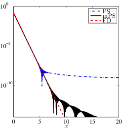
Figure 3: Decay properties of the one column of the discretized Green’s function for the operator $\lambda+\Delta$ with $\lambda=-10$. Here finite difference (FD), pseudo-spectral (PS) and mollified pseudo-spectral (mPS) methods are used. Due to periodic boundary condition only $G(x,0)$ for half of the interval $[0,L/2]$ is shown. Here $L=40,\Delta x=0.02$.

Next we consider the operator $\lambda+\Delta-V(x)$ where $V(x)$ takes the form of a Gaussian function which is not band limited, i.e. $V(x)=10e^{-0.2x^{2}}$, and $\lambda=-10$. The shape of the potential is shown in Fig. 4 (a), and the decay rate for FD, mPS and PS are given in Fig. 4 (b). Similar to the Laplacian case, the addition of the potential function does not modify the behavior of the decay rate. The off-diagonal elements of Green’s function decay exponentially for FD, and super-algebraically for mPS. For PS, the exponential decay only holds up to the consistency error near $10^{-7}$.

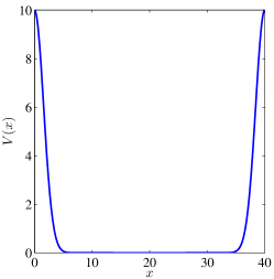
(a)

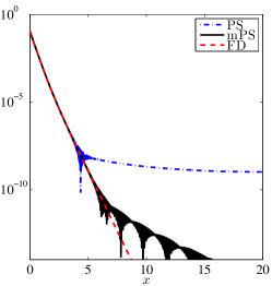
(b)

Figure 4: (a) Potential function $V(x)$. (b) Decay properties of the one column of the discretized Green’s function for the operator $\lambda+\Delta-V(x)$ with $\lambda=-10$. Here finite difference (FD), pseudo-spectral (PS) and mollified pseudo-spectral (mPS) methods are used. Due to periodic boundary condition only $G(x,0)$ for half of the interval $[0,L/2]$ is shown. Here $L=40,N=800$.

Below we systematically measure the dependence of the decay rate with respect to $L$ and $\Delta x$. Although the off-diagonal entries of the discretized Green’s function obtained from the mPS discretization only decay super-algebraically, we expect that the super-algebraic tail is independent of the domain size $L$ with fixed $\Delta x$. We also expect that the decay behavior will become closer to exponential decay when $L$ is fixed and $\Delta x$ is decreasing. In order to verify this, consider $\lambda+\Delta-V(x)$ with $\lambda=-10$, and we measure the exponential decay rate using $G(x,0)$ evaluated at two points $x_{1}=1.0$ and $x_{2}=7.0$, for the mPS method and FD method, respectively. We monitor a quantity $\gamma$ as below

$$\gamma=-\frac{\log G(x_{2},0)-\log G(x_{1},0)}{x_{2}-x_{1}}.$$

$\gamma$ characters the exponential decay rate of $G(x,0)$, and a small value of $\gamma$ indicates sub-exponential decay. Fig. 5 (a) demonstrates the decay rate for increasingly domain size $L$ from $40$ to $400$, with fixed grid size $\Delta x=0.02$. Similarly Fig. 5 (b) demonstrate the decay rate for fixed domain length $L=40$, but with decreasing grid size $\Delta x$ from $0.05$ to $0.005$. Correspondingly the truncation in the Fourier domain $k_{c}$ increases from $62.8$ to $628.3$. We observe that the decay rate of the finite difference scheme is very stable and depends very weakly on both $L$ and $k_{c}$. For mPS scheme, when $\Delta x$ is fixed, the decay rate is lower compared to the decay rate of the finite difference method. This agrees with the super-algebraic tail behavior observed in Fig. 3 and  4. When $L$ is fixed and $\Delta x$ is decreasing and correspondingly $k_{c}$ is increasing, the decay rate improves as $k_{c}$ increases, agreeing with our expectation.

(a)

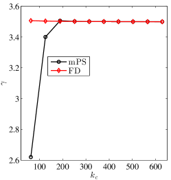
(b)

Figure 5: For $\lambda+\Delta-V(x)$ with $\lambda=-10$, measure the exponential decay rate $\gamma$ for (a) systems with fixed $\Delta x=0.005$ and increasing $L$. (b) systems with fixed $L=40$ and increasing $k_{c}$ (and hence decreasing $\Delta x$).

5 Conclusion

In this paper, we demonstrate that properly discretized Green’s functions for Schrödinger type operators satisfy off-diagonal decay properties. More specifically, for the finite difference discretization, the off-diagonal elements of the discretized Green’s function decay exponentially. For the mollified pseudo-spectral discretization, the off-diagonal elements of the discretized Green’s function decay super-algebraically. In particular, we obtain decay estimates of which the asymptotic decay rate is independent of the domain size $L$ and of the discretization parameter such as the grid spacing. Our analysis is verified by numerical experiments for one-dimensional Schrödinger type operators. Generalization of our estimate to Schrödinger type operators in higher dimensions is straightforward. Our numerical results also indicate that for the widely used pseudo-spectral discretization, due to the non-smoothness of the Laplacian operator at the boundary of the Fourier grid, the asymptotic decay rate of discretized Green’s function is only polynomial with respect to the degrees of freedom. It has been demonstrated that decay estimates of Green’s functions can provide a useful truncation error criterion for designing numerical schemes [BenziBoitoRazouk2013], and our decay estimates can be useful in correcting such error bound especially for operators with large spectral radius. We have assumed uniform grid spacing for both finite difference and pseudo-spectral discretization. This is most suited for smooth and bounded potential $V$. The case with unbounded potential $V$ with isolated singularity points (e.g. in the context of all-electron calculations) will be studied in the future.