Robust Topological Degeneracy of Classical Theories

Abstract

We challenge the hypothesis that the ground states of a physical system whose degeneracy depends on topology must necessarily realize topological quantum order and display non-local entanglement. To this end, we introduce and study a classical rendition of the Toric Code model embedded on Riemann surfaces of different genus numbers. We find that the minimal ground state degeneracy (and those of all levels) depends on the topology of the embedding surface alone. As the ground states of this classical system may be distinguished by local measurements, a characteristic of Landau orders, this example illustrates that topological degeneracy is not a sufficient condition for topological quantum order. This conclusion is generic and, as shown, it applies to many other models. We also demonstrate that certain lattice realizations of these models, and other theories, display a ground state entropy (and those of all levels) that is “holographic”, i.e., extensive in the system boundary. We find that clock and $U(1)$ gauge theories display topological (in addition to gauge) degeneracies.

I Introduction

The primary purpose of the current paper is to show that, as a matter of principle, contrary to discerning lore that is realized in many fascinating systems, e.g., Wen ; wen0 ; Fault-tolerant , the appearance of a topological ground state degeneracy does not imply that these degenerate states are “topologically ordered”, in the sense that local perturbations can be detected without destroying the encoded quantum information Terhal . Towards this end, we introduce various models, including a classical version of Kitaev’s Toric Code Fault-tolerant , that exhibit robust genus dependent degeneracies but are nonetheless Landau ordered. Those models do not harbor long-range entangled ground states that cannot be told apart from one another by local measurements. Rather, they (as well as all other eigenstates) are trivial classical states. Along the way we will discover that these two-dimensional classical models (including rather mundane clock and $U(1)$ gauge like theories with four spin interactions (specifically, Toric Clock and $U(1)$ theories that we will define) may not only have genus dependent symmetries and degeneracies but, for various lattice types, may also exhibit holographic degeneracies that scale exponentially in the system perimeter. Similar degeneracies also appear in classical systems having two spin interactions. Thus, the classical degeneracies that we find may be viewed as analogs of those in quantum models such as the Haah Code model on the simple cubic lattice Haah ; Haah1 ; Haah2 , a nontrivial theory with eight spin interactions that is topologically quantum ordered, and other quantum systems. To put our results in a broader context, we first succinctly review current basic notions concerning the different possible types of order.

The celebrated symmetry-breaking paradigm Landau' ; Landau has seen monumental success across disparate arenas of physics. Its traditional textbook applications include liquid to solid transitions, magnetism, and superconductivity to name only a few examples out of a very vast array. Within this paradigm, distinct thermodynamic phases are associated with local observables known as order parameter(s). In the symmetric phase(s), these order parameters must vanish. However, when symmetries are lifted, the order parameter may become non-zero. Phase transitions occur at these symmetry breaking points at which the order parameter becomes non-zero (either continuously or discontinuously). Landau Landau turned these ideas into a potent phenomenological prescription. Indeed, long before the microscopic theory of superconductivity BCS , Ginzburg and Landau GL wrote down a phenomenological free energy form in the hitherto unknown complex order parameter with the aid of which predictions may be made. Albeit its numerous triumphs, the symmetry-breaking paradigm might not directly account for transitions in which symmetry breaking cannot occur. Pivotal examples are afforded by gauge theories of the fundamental forces and very insightful abstracted simplified renditions capturing their quintessential character, e.g., wegner . Elitzur’s theorem elitzur prohibits symmetry breaking in gauge theories. Another notable example where the symmetry breaking paradigm cannot be directly applied is that of the Berezinskii-Kosterlitz-Thouless transition BKT in two-dimensional systems with a global $U(1)$ symmetry. By the Mermin-Wagner-Hohenberg-Coleman theorem and its extensions MW1 ; MW2 ; MW3 ; MW4 , such continuous symmetries cannot be spontaneously broken in very general two-dimensional systems.

Augmenting these examples, penetrating work illustrated that something intriguing may happen when the quantum nature of the theory is of a defining nature Wen . In particular, strikingly rich behavior was found in Fractional Quantum Hall (FQH) systems Wen ; Tsui ; Laughlin ; Fradkin , chiral spin liquids Wen ; chiral_spin_liquid ; Fradkin , a plethora of exactly solvable models, e.g., Fault-tolerant ; Anyons ; kitaev_review ; Levin-Wen , and other systems. One curious characteristic highlighted in Wen concerns the number of degenerate ground states in FQH fluids wen''' , chiral spin liquids wen' ; wen'' , and other systems. Namely, in these theories, the ground state (g.s.) degeneracy is set by the topology alone. For instance, regardless of general perturbations (including impurities that may break all the symmetries of the Hamiltonian), when placed on a manifold of genus number $g$ (the determining topological characteristic), the FQH liquid at a Laughlin type filling of $\nu=1/q$ (with $q\geq 3$ an odd integer) universally has

$$n^{\sf Laughlin}_{\sf g.s.}=q^{g}$$ (1)

orthogonal ground states wen''' . Equation (1) constitutes one of the best known realization of topological degeneracy. Exact similarity transformations connect the second quantized FQH systems of equal filling when these are placed on different surfaces sharing the same genus FQHE_us . Making use of the archetypal topological quantum phenomenon, the Aharonov-Bohm effect AB , it was argued that, when charge is quantized in units of $(1/q)$ (as it is for Laughlin states), the minimal ground state degeneracy is given by the righthand side of Eq. (1) oshikawa . This may appear esoteric since realizing FQH states on Riemann surfaces is seemingly not feasible in the lab. Recent work sagi proposed the use of an annular superconductor-insulator-superconductor Josephson junction in which the insulator is (an electron-hole double layer) in a FQH state (of an identical filling) for which this degeneracy is not mathematical fiction but might be experimentally addressed. Associated fractional Josephson effects of this type in parafermionic systems were advanced in Fock .

Historically, the robust topological degeneracy of Eq. (1) for FQH systems and its counterparts in chiral spin liquids suggested that such a degeneracy may imply the existence of a novel sort of order — “topological quantum order” present in Kitaev’s Toric Code model Fault-tolerant , Haah’s code Haah ; Haah1 , and numerous other quantum systems wen''' ; wen' ; wen'' ; wen2 — a quantum order for which no local Landau order parameter exists. As we will later review and make precise (see Eq. (3)), in topologically ordered systems, no local measurement may provide useful information.

As it is of greater pertinence to a model analyzed in the current work, we note that similar to Eq. (1), on a surface of genus $g$ the ground state degeneracy of Kitaev’s Toric Code model Fault-tolerant , an example of an Abelian quantum double model representing quantum error correcting codes (solvable both in the ground state sector Fault-tolerant as well as at all temperatures symmetry1 ; symmetry2 ; fragility ), is

$$n^{\sf Toric-Code}_{\sf g.s.}=4^{g}.$$ (2)

Thus, for instance, on a torus ($g=1$), the model exhibits 4 ground states while the system has a unique ground state on a topologically trivial ($g=0$) surface with boundaries. By virtue of a simple mapping symmetry1 ; symmetry2 ; fragility , it may be readily established that an identical degeneracy appears for all excited states; that is the degeneracy of each energy level is an integer multiple of $4^{g}$. Thus, the minimal degeneracy amongst all energy levels is given by $4^{g}$. Same ground state degeneracy msb appears in Kitaev’s honeycomb model Anyons ; kitaev_review . As is widely known, an identical situation occurs in the quantum dimer model QDM ; symmetry1 ; symmetry2 . Invoking the well-known “$n-$ality” considerations of $SU(n)$, leading to a basic spin of 1/2 in $SU(2)$ and a minimal quark charge of 1/3 in $SU(3)$, it was suggested symmetry1 ; symmetry2 that in many systems, fractional charges (quantized in units of $1/n$) are a trivial consequence of the $\mathbb{Z}_{n}$ phase group center structure of a system endowed with an $SU(n)$ symmetry, which is associated with the $n$ states comprising the ground state manifold. This $n$-ality type phase factors and other considerations, prompted Sato sato to suggest the use of topological degeneracy (akin to that of Eqs. (1) and (2)) as a theoretical diagnosis delineating the boundary between the confined and the topological deconfined phases of QCD in the presence of dynamical quarks. Other notable examples include, e.g., the BF action for superconductors (carefully argued to not support a local order parameter vadim ).

References symmetry1 ; symmetry2 examined the links between various concepts surrounding topological order with a focus on the absence of local order parameters. In particular, building on a generalization of Elitzur’s theorem gelitzur ; holography it was shown how to construct and classify theories for which no local order parameter exists both at zero and at positive temperatures; this extension of Elitzur’s theorem unifies the treatment of classical systems, such as gauge and Berezinskii-Kosterlitz-Thouless type theories in arbitrary number of space (or spacetime) dimensions, to topologically ordered systems. Moreover, it was demonstrated that a sufficient condition for the existence of topological quantum order is the explicit presence, or emergence, of symmetries of dimension $d$ lower than the system’s dimension $D$, dubbed $d$-dimensional gauge-like symmetries, and which lead to the phenomenon of dimensional reduction. The topologically ordered ground states are connected by these low-dimensional operator symmetries symmetry1 ; symmetry2 . All known examples of systems displaying topological quantum order host these low dimensional symmetries, thus providing a unifying framework and organizing principle for such an order.

As underscored by numerous pioneers, features such as fractionalization and quasiparticle statistics, e.g., Wen ; Laughlin ; Fault-tolerant ; Anyons ; qps ; brav ; fraction1 ; fraction2 ; fraction3 ; fraction4 ; fraction5 ; fraction6 ; fraction7 ; nayak ; alicea , edge states Fault-tolerant ; Anyons ; nayak ; edge ; wedge , nontrivial entanglement symmetry1 ; symmetry2 ; etqo , and other fascinating properties seem to relate with the absence of local order parameters and permeate topological quantum order. While all of the above features appear and complement the topological degeneracies found in, e.g., the FQH (Eq. (1)), the Toric Code (Eq. (2)), and numerous other systems, it is not at all obvious that one property (say, a topological degeneracy such as those of Eqs. (1) and (2)) implies another attribute (for instance, the absence of meaningful local observables). The current work will indeed precisely establish the absence of such a rigid connection between these two concepts (viz., topological degeneracy is not at odds with the existence of a local order parameter).

We will employ the lack of local order parameters (or, equivalently, an associated robustness to local perturbations) as the defining feature of topological quantum order symmetry1 ; symmetry2 ; fragility . This robustness condition implies that local errors can be detected, and thus corrected, without spoiling the potentially encoded quantum information. To set the stage, in what follows, we consider a set of $n_{\sf g.s.}$ orthonormal ground states$\{|g_{\alpha}\rangle\}_{\alpha=1}^{n_{\sf g.s.}}$ with a spectral gap to all other (excited) states. Specifically symmetry1 ; symmetry2 , a system will be said to exhibit topological order at zero temperature if and only if for any quasi-local operator $\cal V$,

$$\langle g_{\alpha}|{\cal V}|g_{\beta}\rangle=v\ \delta_{\alpha,\beta}+c,$$ (3)

where $v$ is a constant, independent of $\alpha$ and $\beta$, and $c$ is a correction that is either zero or vanishes (typically exponentially in the system size) in the thermodynamic limit. The physical content of Eq. (3) is clear: no possible quantity $\cal V$ may serve as an order parameter to differentiate between the different ground states in the “algebraic language” JW where $\cal V$ is local symmetry1 ; symmetry2 ; holographic . That is, all ground states look identical locally. Similarly, no local operator $\cal V$ may link different orthogonal states – the ground states are immune to all local perturbations. Notice the importance of the physical, and consequently mathematical, language to establish topological order: A physical system may be topologically ordered in a given language but its dual (that is isospectral) is not symmetry1 ; symmetry2 ; holographic .

Expressed in terms of the simple equations that we discussed thus far, the goal of this work is to introduce systems for which the ground state sector has a genus dependent degeneracy (as in Eqs. (1) and (2)) while, nevertheless, certain local observables (or order parameters) $\cal V$ will be able to distinguish between different ground states (thus violating Eq. (3)). Moreover, they will be connected by global symmetry operators as opposed to low-dimensional ones. Our conclusions are generic and, as shown, they apply to many classical models. The paradigmatic counterexample that we will introduce is a new classical version of Kitaev’s Toric Code model Fault-tolerant .

We now turn to the outline of the paper. In Section II, we generalize the standard (quantum) Toric Code model. After a brief review and analysis of the ground states of Kitaev’s Toric Code model (Section III), we exclusively study our classical systems. In Section IV, we extensively study the ground states of the classical variant of the model for different square lattices on Riemann surfaces of varying genus numbers $g\geq 1$. A principal result will be that this and many other classical systems exhibit a topological degeneracy. We will demonstrate that an intriguing holographic degeneracy may appear on lattices of a certain type. As will be explained, topological as well as exponentially large in system linear size (“holographic”) degeneracies can appear in numerous systems, not only in this new classical version of Kitaev’s Toric Code model Noteholo . We further study the effect of lattice defects. The partition function of the classical Toric Code model is revealed in Section V and Appendix A.

In Section VI, we introduce related classical clock models. Generalizing the considerations of Section IV, we will demonstrate that these clock models may exhibit topological or holographic degeneracies. The ensuing analysis is richer by comparison to that of the classical Toric Code model. Towards this end, we will construct a new framework for broadly examining degeneracies. We then derive lower bounds on the degeneracy that are in agreement with our numerical analysis. These bounds are not confined to the ground state sector. That is, all levels may exhibit topological degeneracies (as they do in the classical Toric Code model (Section V)).

In Section VII, we will relate our results to $U(1)$ models and to $U(1)$ lattice gauge theories in particular. The fact that simple lattice gauge systems, that constitute a limiting case of our more general studied models, such as the conventional classical Clock and $U(1)$ lattice gauge theories on general Riemann surfaces (and their Toric Code extensions), exhibit topological (or, in some cases, holographic) degeneracies seems to have been overlooked until now. In Section VIII, we will study honeycomb and triangular lattice systems embedded on surfaces of different genus. In Section IX, we will discuss yet three more regular lattice classical systems that exhibit holographic degeneracies. We summarize our main message and findings in Section X.

Before embarking on the specifics of these various models, we briefly highlight the organizing principle behind the existence of degeneracies in our theories. Irrespective of the magnitude and precise form of the interactions in these theories, the number of independent constraints between the individual interaction terms sets the system degeneracy. As such, the degeneracies that we find are, generally, not a consequence of any particular fine-tuning.

II The general Toric Code Model

We start with a general description of a class of two-dimensional stabilizer models defined on lattices embedded on closed manifolds with arbitrary genus number $g$ (the number of handles or, equivalently, the number of holes). The genus of a closed orientable surface is related to a topological invariant known as Euler characteristic

$$\chi=2-2g,$$ (4)

which, for a general tessellation of that surface, satisfies the (Euler) relation

$$\chi=V-E+F.$$ (5)

In Eq. (5), $V$ is the number of vertices in the closed tessellating polyhedron, or graph, $E$ is the number of edges, and $F$ the number of polygonal faces. Assume that on each of the $E$ edges of the graph there is a spin $S$ degree of freedom, defining a local Hilbert space of size $\dim{\cal{H}}={\sf{d}}_{Q}$, and that on each of the $V$ vertices and $F$ faces we will have a number of conditions to be satisfied by the ground states of a model that we define next.

We now explicitly define, on a general lattice or graph $\Lambda$, the “General Toric Code model”. Towards this end, we consider the Hamiltonian

$$H^{\mu,\nu}=-J\sum_{s}A^{\mu}_{s}-J^{\prime}\sum_{p}B^{\nu}_{p},$$ (6)

where $J$ and $J^{\prime}$ are coupling constants (although it is immaterial, in the remainder of this work we will assume these to be positive). The interaction terms of edges in Eq. (6) are so-called “star” (“$s$”) terms ($A^{\mu}_{s}$) associated with the $V$ vertices (labelled by the letter $i$) and the $F$ “plaquette” (“$p$”) terms ($B^{\nu}_{p}$). In the $S=1/2$ case, these are given by the following products of Pauli operators $\sigma^{\mu}_{ij}$, $\mu,\nu=x,y,z$,

$$A^{\mu}_{s} =\prod_{i\in\,{\sf vertex}(s)}\sigma_{is}^{\mu},$$

$$B^{\nu}_{p} =\prod_{(ij)\in\,{\sf face}(p)}\sigma_{ij}^{\nu}.$$ (7)

The product defining $A^{\mu}_{s}$ spans the spins on all edges $(is)$ that have vertex $s$ as an endpoint, and the plaquette product $B^{\nu}_{p}$ is over all spins lying on the edges $(ij)$ that form the plaquette $p$ (see Fig. 1 for an illustration). A key feature of this system (both the well known Fault-tolerant quantum variant ($\mu=x\neq\nu=z$) as well as, even more trivially, the classical version that we introduce in this paper ($\mu=\nu=z$)) is that each of the bonds $A^{\mu}_{s}$ and $B^{\nu}_{p}$ can assume ${\sf{d}}_{Q}=2S+1=2$ independent values. Apart from global topological constraints symmetry1 ; symmetry2 that we will expand on below, the bonds $\{A^{\mu}_{s}\}$ and $\{B^{\nu}_{p}\}$ are completely independent of one another. Not only, trivially, in the classical but also in the quantum ($q$) rendition of the model Fault-tolerant all of these operators commute with one another. That is $\forall s,p\in\Lambda$,

$$[A^{\mu}_{s},B^{\nu}_{p}]=0.$$ (8)

Figure 1: General Toric Code lattice model with spins $S=1/2$ placed on the edges (bonds). The red cross-shape object corresponds to the star operator $A^{\mu}_{s}$. The plaquette operator $B^{\nu}_{p}$ is depicted in the top-left corner in blue color. Dark solid and dashed lines represent the loops $C_{1}$, $C_{2}$ and $C^{\prime}_{1}$, $C^{\prime}_{2}$, defining the symmetry operators $Z_{1}$, $Z_{2}$, and $X_{1}$, $X_{2}$, respectively.

In the quantum version of the model, these terms commute as the products defining the star and plaquette operators must share an even number of spins. As the individual Pauli operators $\sigma^{x}$ and $\sigma^{z}$ appearing in the product of Eq. (II) anticommute, an even number of such anticommutations trivially gives rise to the commutativity in Eq. (8). Even more simply, one observes that

$$[A^{\mu}_{s},A^{\mu}_{s^{\prime}}]=[B^{\nu}_{p},B^{\nu}_{p^{\prime}}]=0.$$ (9)

Lastly, from Eq. (II), it is trivially seen that

$$(A^{\mu}_{s})^{2}=(B^{\nu}_{p})^{2}=\mathbb{1}.$$ (10)

Apart from a number ($C_{g}^{\Lambda}$) of constraints, Eqs. (8), (9), and (10) completely specify all the relations amongst the operators of Eq. (II). As we will illustrate, $H^{\mu,\nu}$ is a minimal model that embodies all of the elements in Eq. (5) such that its minimum degeneracy will only depend on the genus number $g$. As all terms in the Hamiltonian $H^{\mu,\nu}$ commute with one another, the general Toric Code model can be related quite trivially to a classical model. Intriguingly, as may be readily established by a unitarity transformation (a particular case of the bond-algebraic dualities bond ), the quantum version, which includes Kitaev’s Toric Code model as a particular example, on a graph having $E$ edges spanning the surface of genus $g\geq 1$ is identical symmetry1 ; symmetry2 ; fragility , i.e. is isomorphic, to two decoupled classical Ising chains (with one of these chains having $V$ classical Ising spins and the other chain composed of $F$ Ising spins) augmented by $2(g-1)$ decoupled single Ising spins. Perusing Eq. (6), it is clear that, if globally attainable, within the ground state(s), $|g_{\alpha}\rangle$,

$$A^{\mu}_{s}|g_{\alpha}\rangle=(+1)|g_{\alpha}\rangle\ ,\ B^{\nu}_{s}|g_{\alpha}\rangle=(+1)|g_{\alpha}\rangle,$$ (11)

on all vertices $s$ and faces $p$ and, thus, the ground state energy is $E_{0}=-JV-J^{\prime}F$. The algebraic relations above enable the realization of Eq. (11) for all $s$ and $p$.

We now turn to the constraints that augment Eqs. (8), (9), and (10). For any lattice $\Lambda$ on any closed surface of genus $g\geq 1$, there are $C^{\sf{universal}}_{g\geq 1}=2$ universal constraints given by the equalities

$$\prod_{s}A^{\mu}_{s}=\prod_{p}B^{\nu}_{p}=\mathbb{1}.$$ (12)

For the quantum variant Fault-tolerant no further constraints appear beyond those of Eq. (12) (that is, $C_{g}^{\Lambda}=2$ irrespective of the lattice $\Lambda$). By contrast, for the classical variant of the theory realized on the relatively uncommon “commensurate” lattices, additional constraints will augment those of Eq. (12) (i.e., for classical systems, $C_{g}^{\Lambda}\geq 2$). Invoking the $C_{g}^{\Lambda}$ constraints as well as the trivial algebra of Eqs. (8) and (9), we may transform from the original variables – the spins on each of the $E$ edges – $\{\sigma^{\mu}_{ij}\}$ to new basic degrees of freedom – all ${\sf N}_{{\sf ind.~{}bonds}}$ independent “bonds” $\{A^{\mu}_{s\neq s^{\prime}}\},\{B^{\nu}_{p\neq p^{\prime}}\}$ that appear in the Hamiltonian and $N_{\sf{redundant}}=(E-{\sf N}_{{\sf ind.~{}bonds}})$ remaining redundant spins of the original form $\{\sigma^{\mu}_{ij}\}$ on which the energy does not depend (and thus relate to symmetries). If the bonds $A^{\mu}_{s}$ and $B^{\nu}_{p}$ do not adhere to any constraint apart from that in Eq. (12) then ${\sf N}_{{\sf ind.~{}bonds}}=(V+F-2)$ of the $(V+F)$ bonds in the Hamiltonian of Eq. (6) will be independent of one another. Correspondingly, $N_{\sf{redundant}}=[E-(V+F-2)]=2g$. As all bonds must satisfy the constraint of Eq. (12) and thus ${\sf N}_{{\sf ind.~{}bonds}}\leq(V+F-2)$, the number of redundant spin degrees of freedom $N_{\sf{redundant}}\geq 2g$. In the general case, if there are $(C^{\Lambda}_{g}-2)$ constraints that augment the two restrictions already present in Eq. (12), then we may map the original system of $E$ spins to ${\sf N}_{{\sf ind.~{}bonds}}=(V+F-C^{\Lambda}_{g})$ independent bonds in Eq. (6) and $N_{\sf{redundant}}=(E-{\sf N}_{{\sf ind.~{}bonds}})=2(g-1)+C_{g}^{\Lambda}$ spins that have no impact on the energy. Thus, for genus $g\geq 1$ surfaces, the degeneracy of each energy level is an integer multiple of the minimal degeneracy possible,

$$\min(n_{\sf g.s.})=2^{N_{\sf{redundant}}}=n^{\sf min}_{\sf g.s.}\times 2^{C^{\Lambda}_{g}-2},$$ (13)

with $n^{\sf min}_{\sf g.s.}=4^{g}$. Equation (13) will lead to a global redundancy factor in the partition function ${\cal Z}={\sf Tr}\exp(-\beta H^{\mu,\nu})$ with $\beta$ the inverse temperature.

We now focus on the ground state sector. If there are no constraints apart from Eq. (12), then to obtain the ground states it suffices to make certain that ${\sf N}_{{\sf ind.~{}bonds}}$ of the bonds are unity in a given state. Once that occurs, we are guaranteed a ground state in which each bond in the Hamiltonian of Eq. (6) is maximized (i.e., Eqs. (11) are satisfied). A smaller number of bonds fixed to one will not ensure that only ground states may be obtained. Thus the values of all ${\sf N}_{{\sf ind.~{}bonds}}$ independent bonds need to be fixed in order to secure a minimal value of the energy. The lower bound of the degeneracy on each level (Eq. (13)) is saturated for the ground state sector where it becomes an equality. That is, very explicitly, the ground state degeneracy is given by

$$n^{\sf General~{}Toric-Code}_{\sf g.s.}=4^{g}\times 2^{C^{\Lambda}_{g}-2}.$$ (14)

The equalities of Eqs. (13) and (14) are basic facts that will be exploited in the present article. The degeneracy of Eq. (14) is in accord with the general result

$$n^{\sf{g\geq 1}}_{\sf g.s.}={\sf{d}}_{Q}^{-\chi+(C^{\Lambda}_{g}-C^{\Lambda}_{1})}n^{\sf{g=1}}_{\sf g.s.},$$ (15)

and differs from that of Kitaev’s Toric Code model Fault-tolerant (Eq. (2)) by a factor of $2^{C^{\Lambda}_{g}-2}$. As each of the $C^{\Lambda}_{g}$ constraints as well as increase in genus number leads to a degeneracy of the spectrum, a simple “correspondence maxim” follows: it must be that we may associate a corresponding independent set of symmetries with any individual constraint. Similarly, as Eqs. (13, 14) attest, elevating the genus number $g$ must introduce further symmetries. Thus, the global degeneracy of Eq. (13) is a consequence of all of these symmetries.

Given Eq. (6) it is readily seen that the system has a gap of magnitude $\Delta=4(J+J^{\prime})$ between the ground state $E_{0}$ and the lowest lying excited state $E_{1}$. All energy levels $E_{\ell}$, defining the spectrum of $H^{\mu,\nu}$, are quantized in integer multiples of $J$ and $J^{\prime}$.

III Ground states of the quantum Toric Code model

In Kitaev’s Toric Code model Fault-tolerant the symmetries associated with the constraints of Eq. (12) are rather straightforward, and cogently relate to the topology of the surface on which the lattice is embedded. An illustration for the square lattice is depicted in Fig. 1. For such a model on a simple torus (i.e., one with genus $g=1$), the four canonical symmetry operators are

$$Z^{q}_{1,2}=\prod_{(ij)\in C_{1,2}}\sigma_{ij}^{z}\ ,\ X^{q}_{1,2}=\prod_{(ij)\in C^{\prime}_{1,2}}\sigma_{ij}^{x}.$$ (16)

These two sets of non-commuting operators Fault-tolerant

$$\{X^{q}_{1},Z^{q}_{1}\}=\ 0 \ =\{X^{q}_{2},Z^{q}_{2}\},$$

$$\left[X^{q}_{1},X^{q}_{2}\right]=\ 0 \ =\left[Z^{q}_{1},Z^{q}_{2}\right],$$

$$\left[X^{q}_{1},Z^{q}_{2}\right]=\ 0 \ =\left[X^{q}_{2},Z^{q}_{1}\right],$$ (17)

realize a $\mathbb{Z}(2)\times\mathbb{Z}(2)$ symmetry and ensure a four-fold degeneracy (or, more generally a degeneracy that is an integer multiple of four) of the whole spectrum.

To see this, we may, for instance, seek mutual eigenstates of the Hamiltonian $H^{x,z}$ along with the two symmetries $Z^{q}_{1}$ and $Z^{q}_{2}$ with which it commutes. Noting the algebraic relations amongst the above operators, a moment’s reflection reveals that a possible candidate for a normalized ground state is given by

$$|g_{1}\rangle=\frac{1}{\sqrt{2}}\prod_{s}\left(\frac{\mathbb{1}+A_{s}^{x}}{\sqrt{2}}\right)|{\bf F}\rangle,$$ (18)

where $\sigma^{z}_{ij}|{\bf F}\rangle=|{\bf F}\rangle$, for all $E$ edges, and $\langle{\bf F}|{\bf F}\rangle=1$. This corresponds to $Z^{q}_{1,2}|g_{1}\rangle=|g_{1}\rangle$. Now, because $X^{q}_{1,2}$ are symmetries, by the algebraic relations of Eq. (III), the three additional orthogonal states

$$|g_{2}\rangle=X_{1}^{q}|g_{1}\rangle\ ,\ |g_{3}\rangle=X_{2}^{q}|g_{1}\rangle\ ,\ |g_{4}\rangle=X_{1}^{q}X_{2}^{q}|g_{1}\rangle,$$ (19)

are the remaining ground states. That is, the $C^{\Lambda}_{g=1}=2$ lattice ($\Lambda$) independent constraints of the quantum model (Eq. (12)) correspond to the $2$ sets of symmetry operators associated with the $\gamma=1,2$ toric cycles ($\{Z^{q}_{\gamma},X^{q}_{\gamma}\}$) of Eq. (16). This correspondence is in agreement with the simple maxim highlighted above. The symmetry operators $X^{q}_{1}$ and $Z^{q}_{1}$ are independent (and trivially commute) with the symmetry operators $X^{q}_{2}$ and $Z^{q}_{2}$. Notice that in the spin $(\sigma^{\mu}_{ij}$) language the ground states above are entangled, and they are connected by $d=1$ symmetry operators symmetry1 ; symmetry2 . Moreover, the anyonic statistics of its excitations is linked to the entanglement properties of those ground states symmetry1 ; symmetry2 . As mentioned above, the model can be trivially related, by duality, to two decoupled classical Ising chains so that in the dual language the mapped ground states are unentangled symmetry1 ; symmetry2 .

For a Riemann surface of genus $g$, we may write down trivial extensions of Eqs. (16) for the $(2g)$ cycles circumnavigating the $g$ handles of that surface. That is, instead of the four operators of Eq. (16), we may construct $2g$ operators pairs with each of these pairs associated with a particular handle $h$ (where $1\leq h\leq g$), containing the four operators $\{Z^{q}_{\gamma,h}\}$ and $\{X^{q}_{\gamma,h}\}$ with $\gamma=1,2$. A generalization of Eqs. (III) leads to an algebra amongst the $2g$ independent pairs of symmetry operators. The multiplicity of independent symmetries leads to the first factor in Eq. (14). The number of constraints is, in the quantum case, lattice independent and given by $C^{\Lambda}_{g\geq 1}=2$ (there are no constraints beyond those in Eq. (12)). It is rather straightforward to establish that when $g=0$ (i.e., for topologically trivial surfaces), the ground state of the quantum model is unique. Putting all of these pieces together, the well known degeneracy of Eq. (2) follows.

IV Ground states of the classical Toric Code model

We now finally turn to the examination of the ground states of the classical rendering of Eq. (6) in which only a single component $\mu=\nu=z$ of all spins appears. We will explain how the degeneracy of Eqs. (13) and (14) emerges. The upshot of our analysis, already implicitly alluded to above, consists of two main results:

$\bullet$ In the most frequent lattice realization of this classical model, its degeneracy will still be given by Eq. (2), i.e., $4^{g}$. That is, in the most common of geometries, the number of ground states will depend on topology alone (i.e., the genus number $g$ of the embedding manifold). For arbitrary square lattice or graph, as our considerations universally mandate, the minimal possible ground state degeneracy will be given by the topological figure of merit of Eq. (2).

$\bullet$ In the remaining lattice realizations, the degeneracy of the system will typically be holographic. That is, in these slightly rarer lattices, the ground state degeneracy will scale as ${\cal{O}}(2^{L})$ where $L$ is the length of one of the sides of the two-dimensional lattice.

As will be seen, for the square lattice, depending on the parity of the length of the lattice sides, the number of constraints $C^{\Lambda}_{g}$ may exceed its typical value of two. This will then lead to an enhanced degeneracy vis a vis the minimal possible value of $4^{g}$. In the next subsection we first broadly sketch the constraints and symmetries of the classical system. As it will be convenient to formulate our main result via the “correspondence maxim”, we will then proceed to explicitly relate the constraints and symmetries to one another. The $symmetry\leftrightarrow constraint$ consonance, along with Eqs. (13) and (14), will then rationalize all of the degeneracies found for general square lattices embedded on Riemann surfaces of arbitrary genus number. Exhaustive calculations for these degeneracies will then be reported in the subsections that follow.

IV.1 Symmetries and constraints

We next list the general symmetries and constraints of the classical Toric Code model in square lattices of varying sizes. Consider first a lattice $\Lambda$ of size $L_{x}\times L_{y}$ on a torus (i.e., having $V=L_{x}L_{y}$ vertices and $E=2L_{x}L_{y}$ edges). We will then examine more general lattices of arbitrary genus $g$. The square lattice on the torus will be categorized as being one of two types:

$$\begin{cases}\text{Type I},&\text{$L_{x}\neq L_{y}$ where at least}\\ &\text{one of $L_{x}$ or $L_{y}$ is odd}\\ \text{Type II},&\text{otherwise}.\\ \end{cases}$$ (20)

Type I lattices, as defined for the $g=1$ case above and their generalizations for higher genus numbers $g>1$, only admit two constraints $C^{\Lambda}_{g}$ and thus by the correspondence maxim only two symmetries. For these lattices, we will show that the ground state degeneracy is $4^{g}$. By contrast, Type II lattices have a larger wealth of constraints, $C^{\Lambda}_{g}>2$, and therefore a larger number of symmetries and a degeneracy higher than $4^{g}$.

Figure 2: Dotted lines represent the rotated lattice $\Lambda^{\prime}$. The spin degrees of freedom $\vec{\sigma}$ reside on the vertices of the rotated bipartite lattice $\Lambda^{\prime}$, formed out of two sublattices $\Lambda_{+}$ and $\Lambda_{-}$.

The centers of all nearest neighbor edges on the square lattice (of lattice constant $a$) form yet another square lattice $\Lambda^{{}^{\prime}}$ (of lattice constant $a/\sqrt{2}$) at an angle of $45^{\circ}$ relative to the original lattice (Fig. 2). The spins are located at the vertices of the rotated square lattice $\Lambda^{{}^{\prime}}$. In order to describe the symmetries and constraints of this system, let us denote the two (standard) sublattices of the square lattice $\Lambda^{{}^{\prime}}$ by $\Lambda_{\pm}$. That is, both $\Lambda_{+}$ and $\Lambda_{-}$ are, on their own, square lattices with $\Lambda^{{}^{\prime}}=\Lambda_{+}\cup\Lambda_{-}$ and $\Lambda_{+}\cap\Lambda_{-}=\emptyset$. Let us furthermore denote the sites of $\Lambda_{\pm}$ by ${\imath_{\pm}}$, respectively.

With these preliminaries, it is trivial to verify that

$$T^{x}_{+}=\prod_{\imath_{+}\in\Lambda_{+}}\sigma^{x}_{\imath_{+}},\ \$$

$$T^{x}_{-}=\prod_{\imath_{-}\in\Lambda_{-}}\sigma^{x}_{\imath_{-}},\ \$$ (21)

are, universally, both symmetries of the classical ($\mu=\nu=z$) version of the Hamiltonian of Eq. (6). Most square lattices (those of Type I in Eq. (20)) will only exhibit the two symmetries of Eq. (IV.1). The more commensurate Type II lattices admit diagonal contours (connecting nearest neighbors of sites $\imath$ of $\Lambda^{{}^{\prime}}$) that close on themselves before threading all of the lattice sites of $\Lambda^{{}^{\prime}}$. That is, in Type II lattices, it is possible to find diagonal loops $\Gamma_{m}$ at a constant $45^{\circ}$ angle (or a more non-trivial alternating contour) that contain only a subset of all sites of $\Lambda^{{}^{\prime}}$ (or, equivalently, a subset of all edges $(ij)$ of the original square lattice $\Lambda$). Associated with each such independent contour $\Gamma_{m}$, there is a symmetry operator,

$$T^{x}_{m}=\prod_{\imath\in\Gamma_{m}}\sigma^{x}_{\imath},$$ (22)

augmenting the symmetries of Eq. (IV.1).

The form of the symmetries suggests the distinction between Type I and Type II lattices on general surfaces. On Type II lattices, it is possible to find, at least, one diagonal contour $\Gamma_{m}$ that contains a subset of all edges $(ij)$ of the lattice $\Lambda$. Conversely, due to the lack of the requisite lattice commensurability, on Type I lattices, it is impossible to find any such contour.

We now turn to the constraints associated with Type I and II lattices. These are in one-to-one correspondence with the symmetries of Eqs. (IV.1) and (22). Specifically for Type I lattices, the only universal constraints present are those of Eq. (12) which we rewrite again for clarity,

$${\cal{C}}_{+}:~{}~{}\prod_{s}A^{z}_{s}=1,$$

$${\cal{C}}_{-}:~{}~{}\prod_{p}B^{z}_{p}=1.$$ (23)

These two constraints match the two symmetries of Eq. (IV.1). In the case of the more commensurate lattices $\Lambda$, additional constraints appear. In order to underscore the similarities to the symmetries of Eq. (22), we will now aim to briefly use the same notation concerning the lattice $\Lambda^{{}^{\prime}}$. Within the framework highlighted in earlier sections, the spin products $\{A^{z}_{s}\}$ and $\{B^{z}_{p}\}$ of Eq. (II) are associated with geometrical objects that look quite different (i.e., “stars” and “plaquettes”), see Fig. 1. If we now label the plaquettes of $\Lambda^{{}^{\prime}}$ by ${\mathcal{P}}$ then, we may, of course, trivially express Eq. (6) as a sum of local terms,

$$H=-J\sum_{{\mathcal{P}}}W_{{\mathcal{P}}}-J^{\prime}\sum_{{\mathcal{P}^{\prime}}}W_{{\mathcal{P}^{\prime}}},$$ (24)

where $W_{{\mathcal{P}}}=\prod_{\imath\in{{\mathcal{P}}}}\sigma^{z}_{\imath}$ are the products of all Ising spins at sites $\imath$ belonging to plaquette ${{\mathcal{P}}}$. This trivial description renders the original star and plaquette terms of Eq. (6) on a more symmetric footing, see Fig. 2.

Associated with each of the symmetries of Eq. (22) there is a corresponding constraint,

$${\cal{C}}_{m}:~{}~{}\prod_{\imath\in\Gamma_{m}}W_{m}=1.$$ (25)

In accordance with our earlier maxim, insofar as counting is concerned, we have the following correspondence between the symmetries and the associated constraints,

$$\begin{cases}T^{x}_{+}\leftrightarrow{\cal{C}}_{+},\\ T^{x}_{-}\leftrightarrow{\cal{C}}_{-},\\ T^{x}_{m}\leftrightarrow{\cal{C}}_{m}.\\ \end{cases}$$ (26)

In Type I systems, wherein only the $C^{\Lambda}_{g}=2$ universal constraints appear, the degeneracy of the spectrum is exactly $4^{g}$. In Type II lattices, $C_{g}^{\Lambda}>2$ (with the difference of $(C_{g}^{\Lambda}-2)$ equal to the number of additional independent contours $\Gamma_{m}$ that do not contain all edges of the original lattice $\Lambda$) and, as Eq. (14) dictates, the ground state degeneracy exceeds the minimal value of $4^{g}$ multiplied by two raised to the power of the number of the additional independent loops.

Figure 3: A square lattice with $8$ spins along with its embedding on a torus. Because of periodic boundary conditions, spins on boundary edges (dashed-blue) display numbers identical to those in the bulk. In this figure $A_{s}=A^{z}_{s}$ and $B_{p}=B^{z}_{p}$. In the right panel, each edge has been labeled according to the left panel, and the solid red squares represent the vertices labeled by $A_{s}$. Since $B_{3}$ and $B_{4}$ are respectively behind $B_{1}$ and $B_{2}$, we cannot see them here.

IV.2 Ground state degeneracy on $g=1$ surfaces

Thus far, our discussion has been quite general and, admittedly, somewhat abstract. We now turn to simple concrete examples. We first consider the classical Toric Code model on a simple torus (i.e., a surface with genus $g=1$), and examine small specific square lattices of dimension $L_{x}\times L_{y}$. We find that for general lattices $\Lambda$ (with reference to Eq. (20)), the total number of independent constraints is

$$C^{\Lambda}_{g=1}=\begin{cases}2,&\text{$\Lambda$ is a Type I lattice}\\ &\\ 2\min\{L_{x},L_{y}\},&\text{$\Lambda$ is a Type II lattice.}\\ \end{cases}$$ (27)

Thus, from Eq. (14), our two earlier stated main results follow: while for the more “incommensurate” Type I lattices, the degeneracy will be “topological” (i.e., given by $4^{g}$), for Type II lattices, the degeneracy will be “holographic” (viz., the degeneracy will be exponential in the smallest of the edges along the system boundaries). As discussed in Section IV.1, the additional constraints in Type II lattices are of the form of Eq. (25). Expressed in terms of the four spin interaction terms $A^{z}_{s}$ and $B^{z}_{p}$ of Eq. (6), a constraint of the form of Eq. (25) states that there is a subset $\Gamma_{m}\subset\Lambda$ for which $\prod_{s,p\in\Gamma_{m}}A^{z}_{s}B^{z}_{p}=1$. An illustration of a constraint of such a type is provided, e.g. in Fig. 3. Here, by virtue of the defining relations of Eq. (II), the product,

$$A^{z}_{1}B^{z}_{1}A^{z}_{4}B^{z}_{4}=1.$$ (28)

Similarly, in panel a) of Fig. 4, colored arrows are drawn along the diagonals. These colors code the constraints on the specific $A_{s}^{z}$ and $B_{p}^{z}$ interaction terms. For example, along the green arrows,

$$A^{z}_{1}B^{z}_{1}A^{z}_{4}B^{z}_{4}=1\,\,\,\,\,\,\,\,\,\,\text{green (dashed)},$$ (29)

and the constraints associated with the other diagonals

$$A^{z}_{2}B^{z}_{2}A^{z}_{3}B^{z}_{3} = 1\,\,\,\,\,\,\,\,\,\,\text{brown (dashed-dotted)},$$

$$A^{z}_{2}B^{z}_{1}A^{z}_{3}B^{z}_{4} = 1\,\,\,\,\,\,\,\,\,\,\text{red (dashed-doubled-dotted)},$$

$$A^{z}_{1}B^{z}_{2}A^{z}_{4}B^{z}_{3} = 1\,\,\,\,\,\,\,\,\,\,\text{black (dotted)}.$$ (30)

Figure 4: a) Lattice of size $L_{x}=2$, $L_{y}=2$, $E=8$ and b) $L_{x}=2$, $L_{y}=3$, $E=12$. Diagonal lines with arrows represent possible paths realizing constraints on $A_{s}=A^{z}_{s}$ and $B_{p}=B^{z}_{p}$.

We provide another example in panel b) of Fig. 4. The simplest visually appealing realization of Eq. (25) is that of the subset $\Gamma_{m}$ being a trivial closed diagonal loop. Composites (i.e., products) of independent constraints of the form of Eq. (25) are, of course, also constraints. We aim to find the largest number $(C^{\Lambda}_{g}-2)$ of such independent constraints. Non-trivial constraints formed by the product of bonds along real-space diagonal lines may appear. For example, in Fig. 3, the product $A^{z}_{1}B^{z}_{1}A^{z}_{3}B^{z}_{2}=1$ is precisely such a constraint. These constraints are more difficult to determine due to the periodic boundary conditions. Generally, not all constraints are independent of each other (e.g., multiplying any two constraints yield a new constraint). The number of independent constraints, $C^{\Lambda}_{g}$ may be generally found by calculating the “modular rank” of the linear equations formed by taking the logarithm of all constraints found. The qualified “modular” appears here as the $A^{z}_{s}$ and $B^{z}_{p}$ eigenvalues may only be $(\pm 1)$ and thus, correspondingly, their phase is either $0$ or $\pi$. Many, yet generally, not all, of the $C^{\Lambda}_{g}$ independent constrains are naturally associated with products along the 45^∘ lattice diagonals (as it appears on the torus). Table 1 lists the numerically computed ground state degeneracies for numerous lattices of genus $g=1$. All of these are concomitant with Eq. (27).

Type	$L_{x}$	$L_{y}$	$E$	$C_{g=1}^{\Lambda}$	$n_{\sf{g.s.}}$
I	3	2	12	2	4
	5	2	20	2	4
	4	3	24	2	4
	5	3	30	2	4
II	2	2	8	4	$4\times 2^{2}$
	4	2	16	4	$4\times 2^{2}$
	6	2	24	4	$4\times 2^{2}$
	3	3	18	6	$4\times 2^{4}$
	4	4	32	8	$4\times 2^{6}$

Table 1: Computed ground state degeneracy ($n_{\sf{g.s.}}$) for the classical Toric Code for different lattice sizes with genus one. Type I corresponds to the case $L_{x}\neq L_{y}$ where at least one of them is odd. We put any other possibility under Type II which in general covers the case $L_{x}\neq L_{y}$ where both $L_{x}$ and $L_{y}$ are even plus all cases with $L_{x}=L_{y}$. In this table, $C_{g=1}^{\Lambda}$ denotes the number of independent constraints (see text).

IV.3 Construction of ground states

Given the symmetry operators of Eqs. (IV.1) and (22), we may rather readily write down all ground states of the system. Denote the ferromagnetic ground state (i.e., one with all spins up ($|\!\uparrow\rangle_{(ij)}$) on all edges $(ij)$) by

$$|{\bf F}\rangle\equiv\prod_{(ij)}|\uparrow\rangle_{(ij)};$$ (31)

then, the four ground states of Type I lattices are

$$|G_{n_{+},n_{-}}\rangle=(T^{x}_{+})^{n_{+}}(T^{x}_{-})^{n_{-}}|{\bf F}\rangle,$$ (32)

where $n_{\pm}=0,1$. Clearly, since $(T^{x}_{\pm})^{2}=1$, only the parity of the integers $n_{\pm}$ is important. As (i) $[T^{x}_{\pm},H]=0$ and (ii) the ferromagnetic state $|{\bf F}\rangle$ minimizes the energy in Eq. (6), it follows that all four binary strings $(n_{+},n_{-})=(0,0),(0,1),(1,0),(1,1)$ in Eq. (32) lead to $n_{\sf{g.s.}}=2^{2}=4$ ground states. The situation for Type II lattices is a trivial extension of the above. That is, if there are $(C_{g=1}^{\Lambda}-2)$ additional independent symmetries $T^{x}_{m=1},T^{x}_{m=2},\cdots,T^{x}_{m=(C_{g=1}^{\Lambda}-2)}$ of the form of Eq. (22) then, with the convention of Eq. (31), the ground states will be of the form

$$|G_{n_{+},n_{-},n_{1},n_{2},\cdots,n_{C_{g=1}^{\Lambda}-2}}\rangle=(T^{x}_{+})^{n_{+}}(T^{x}_{-})^{n_{-}}(T^{x}_{1})^{n_{1}}$$

$$\hskip 56.9055pt\times(T^{x}_{2})^{n_{2}}\cdots(T^{x}_{C_{g=1}^{\Lambda}-2})^{n_{C_{g=1}^{\Lambda}-2}}|{\bf F}\rangle,$$ (33)

with $2^{C_{g=1}^{\Lambda}}$ binary strings $(n_{+},n_{-},n_{1},n_{2},\cdots,n_{C_{g=1}^{\Lambda}-2})$, where $n_{m}=0,1$. These strings span all possible $n_{\sf{g.s.}}=2^{C_{g=1}^{\Lambda}}$ orthogonal ground states.

Given the set of all orthonormal ground states $\{|g_{\alpha}\rangle\}_{\alpha=1}^{n_{\sf{g.s.}}}$, it is possible to find quasi-local operators ${\cal V}$ composed of $\sigma^{z}_{ij}$ “operators” on a small number of edges such that

$$\langle g_{\alpha}|{\cal V}|g_{\alpha}\rangle=v_{\alpha}$$ (34)

assumes different values $v_{\alpha}$ in, at least, two different ground states. Equation (34) highlights that the expectation value of ${\cal V}$ is not state independent. In other words, Eq. (3) symmetry1 ; symmetry2 ; fragility is violated. Thus, our classical system is, rather trivially, not topologically ordered .

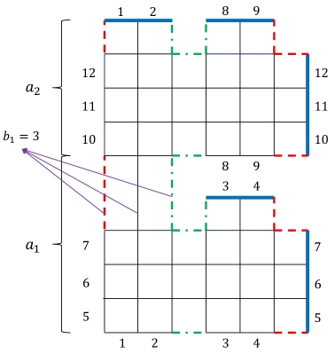
Figure 5: A genus two ($g=2$) lattice. Identical bonds are labeled by the same number (as a result of periodic boundary conditions). Thick solid (blue) lines represent the boundary. The two plaquettes with $8$ bonds are shown by dashed (red) and dashed-dotted (green) lines.

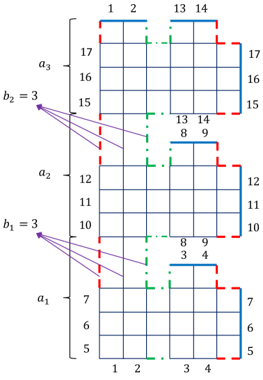
Figure 6: A genus three ($g=3$) lattice. Identical bonds are labeled by the same number (as a result of periodic boundary conditions). Thick solid (blue) lines represent the boundary. The two plaquettes with $12$ bonds are shown by dashed (red) and dashed-dotted (green) lines.

IV.4 Ground state degeneracy on $g>1$ surfaces

Having understood the case of the simple torus ($g=1$), we will now study lattices on surfaces $\Sigma$ of genus $g\geq 2$. We first explain how to construct a finite size lattice of genus $g$ Ising-genus>1 . Such lattices on genus $g$ ($g\geq 2$) surfaces may be formed by “stitching together” $g$ simple parts $a_{j}$, $j=1,\cdots,g$, each of which largely looks like that of a simple torus (i.e., each region $a_{j}$ represents a set of vertices, edges and faces of Type I or II in the notation of Eq. (20)), via $(g-1)$ “bridges” $\{b_{j}\}^{g-1}_{j=1}$. In Figs. 5, and 6, the integer number $b_{j}$ denotes the number of edges that regions $a_{j}$ and $a_{j+1}$ share.

To lucidly illustrate the basic construct, we start first with a $g=2$ lattice. In Fig. 5, identical edges are labeled by the same number as a consequence of the periodic boundary conditions. Here, there are $E=96$ edges, $V=48$ vertices, and $F=46$ plaquettes. As in the case of the simple torus ($g=1$), the typical vertices are endpoints of four edges. Similarly, in Fig. 5, all plaquettes (with the exception of two) are comprised of four edges as in the situation of the simple torus. The exceptional cases are colored green (dashed-dotted) and red (dashed). As seen in the figure, the lattice may be splintered into two regions (labeled by $a_{1}$ and $a_{2}$) where one end of some of the bonds belonging to $a_{1}$ are connected to $a_{2}$ as shown and labeled in the picture under $b_{1}$. Each of the regions $a_{1}$ and $a_{2}$ looks, by itself, like a square lattice on a genus $g=1$ surface. Generally, the regions $a_{1}$ and $a_{2}$ may be composed of a different number of edges. Employing the taxonomy of Eq. (20), we may classify these regions $\{a_{j}\}_{j=1}^{g}$ to be of either Type I or II. We remark that the number of edges $b_{1}$ must be always at least one less than the minimum of the number of bonds of $a_{1}$ and $a_{2}$ along the horizontal ($x$) axis. This algorithm trivially generalizes to higher genus number. The cartoon of Fig. 6 represents a lattice with $g=3$.

A synopsis of our numerical results for the ground state degeneracy for surfaces of genus $2\leq g\leq 5$ appears in Table 2. The ground state degeneracy depends on the type of each $a_{j}$ and the number of bonds of each $b_{j}$. When all fragments $\{a_{j}\}$ are of Type I and are inter-connected by only single common edges, the degeneracy attains will its minimal possible value (Eq. (14)) of $4^{g}$ .

$g$

$E$

$n_{\sf{g.s.}}$

Type

$a_{1}$

$b_{1}$

$a_{2}$

$b_{2}$

$a_{3}$

$b_{3}$

$a_{4}$

$b_{4}$

$a_{5}$

2

8

$4^{g}$

2 I

2$\times$1

1

2$\times$1

10

$4^{g}$

2 I

3$\times$1

1

2$\times$1

12

$4^{g}$

2 I

3$\times$1

1

3$\times$1

16

$4^{g}$

2 I

3$\times$2

1

2$\times$1

18

$4^{g}$

2 I

3$\times$2

1

3$\times$1

24

$4^{g}$

2 I

3$\times$2

1

3$\times$2

24

$4^{g}$

2 I

5$\times$2

1

2$\times$1

12

$4^{g}\times 2$

2 I

3$\times$1

2

3$\times$1

12

$4^{g}\times 2$

II+I

2$\times$2

1

2$\times$1

14

$4^{g}\times 2$

II+I

2$\times$2

1

3$\times$1

20

$4^{g}\times 2$

I+II

3$\times$2

1

2$\times$2

20

$4^{g}\times 2$

II+I

4$\times$2

1

2$\times$1

22

$4^{g}\times 2$

II+I

4$\times$2

1

3$\times$1

24

$4^{g}\times 2$

2 I

3$\times$2

2

3$\times$2

24

$4^{g}\times 2$

II+I

3$\times$3

2

3$\times$1

16

$4^{g}\times 2^{3}$

2 II

2$\times$2

1

2$\times$2

24

$4^{g}\times 2^{3}$

II+I

3$\times$3

1

3$\times$1

24

$4^{g}\times 2^{3}$

2 II

4$\times$2

1

2$\times$2

3

12

$4^{g}$

3 I

2$\times$1

1

2$\times$1

1

2$\times$1

14

$4^{g}$

3 I

3$\times$1

1

2$\times$1

1

2$\times$1

16

$4^{g}$

3 I

3$\times$1

1

3$\times$1

1

2$\times$1

16

$4^{g}$

3 I

3$\times$1

2

3$\times$1

1

2$\times$1

18

$4^{g}$

3 I

3$\times$1

1

3$\times$1

1

3$\times$1

18

$4^{g}$

3 I

3$\times$1

2

3$\times$1

1

3$\times$1

18

$4^{g}$

3 I

3$\times$1

1

3$\times$1

2

3$\times$1

18

$4^{g}$

3 I

3$\times$1

2

3$\times$1

2

3$\times$1

20

$4^{g}$

3 I

3$\times$2

1

2$\times$1

1

2$\times$1

24

$4^{g}$

3 I

3$\times$2

1

3$\times$1

1

3$\times$1

24

$4^{g}$

3 I

3$\times$2

2

3$\times$1

2

3$\times$1

16

$4^{g}\times 2$

2 I+II

2$\times$1

1

2$\times$1

1

2$\times$2

18

$4^{g}\times 2$

2 I+II

3$\times$1

1

2$\times$1

1

2$\times$2

20

$4^{g}\times 2$

2 I+II

3$\times$1

1

3$\times$1

1

2$\times$2

20

$4^{g}\times 2^{2}$

2 II+I

2$\times$2

1

2$\times$2

1

2$\times$1

22

$4^{g}\times 2^{2}$

2 II+I

2$\times$2

1

2$\times$2

1

3$\times$1

24

$4^{g}\times 2^{4}$

3 II

2$\times$2

1

2$\times$2

1

2$\times$2

4

16

$4^{g}$

4 I

2$\times$1

1

2$\times$1

1

2$\times$1

1

2$\times$1

18

$4^{g}$

4 I

2$\times$1

1

2$\times$1

1

2$\times$1

1

3$\times$1

24

$4^{g}$

4 I

3$\times$2

1

2$\times$1

1

2$\times$1

1

2$\times$1

20

$4^{g}\times 2$

II+3 I

2$\times$2

1

2$\times$1

1

2$\times$1

1

2$\times$1

5

20

$4^{g}$

5 I

2$\times$1

1

2$\times$1

1

2$\times$1

1

2$\times$1

1

2$\times$1

24

$4^{g}\times 2$

II + 4 I

2$\times$2

1

2$\times$1

1

2$\times$1

1

2$\times$1

1

2$\times$1

Table 2: Computed ground state degeneracy ($n_{\sf{g.s.}}$) for square lattices with $g>1$. The $g$ denotes “genus” (see text).

If, in Eq. (6), we set $J$ to zero, we will obtain the Hamiltonian of the Ising gauge model. As this theory does not have a star term, this Hamiltonian involves more symmetries and, therefore, one expects the ground state subspace to have a larger degeneracy. We numerically verified it to be $n^{\sf gauge}_{\sf g.s.}=4^{g}\times 2^{\sf N_{site}-1}$-fold degenerate (${\sf N_{site}}=E/2$) local-gauge-Ising .

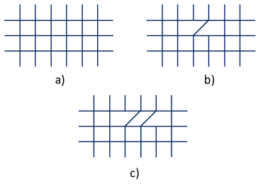
Figure 7: Sketch of a part of a square lattice a) with two types of defects b) and c). The defective lattices in b) and c) have one bond less than in a).

$g$	$E$	$n_{\sf{g.s.}}$	Type	$a_{1}$	$b_{1}$	$a_{2}$	$b_{2}$	$a_{3}$	$b_{3}$	$a_{4}$
1	11	$4^{g}$	I	3$\times$2 $\star$
	15	$4^{g}$	II	4$\times$2 $\star$
	19	$4^{g}$	I	5$\times$2 $\star$
	23	$4^{g}$	I	6$\times$2 $\star$
	23	$4^{g}$	I	4$\times$3 $\star$
	16	$4^{g}\times 2$	II	3$\times$3 $2\star$
	17	$4^{g}\times 2$	II	3$\times$3 $\star$
	19	$4^{g}\times 2$	I	5$\times$2 $\star\star$
	22	$4^{g}\times 2$	I	6$\times$2 $2\star$
2	15	$4^{g}$	2 I	3$\times$2 $\star$	1	2$\times$1
	17	$4^{g}$	2 I	3$\times$2 $\star$	1	3$\times$1
	21	$4^{g}$	2 I	4$\times$2 $\star$	1	3$\times$1
	22	$4^{g}$	2 I	3$\times$2 $\star$	1	3$\times$2 $\star$
	23	$4^{g}$	2 I	3$\times$2 $\star$	1	3$\times$2
	23	$4^{g}$	2 II	4$\times$2 $\star$	1	2$\times$2
	23	$4^{g}$	II+I	3$\times$3 $\star$	2	3$\times$1
	23	$4^{g}$	2 I	5$\times$2 $\star$	1	2$\times$1
	23	$4^{g}\times 2$	II+I	3$\times$3 $\star$	1	3$\times$1
3	19	$4^{g}$	3 I	3$\times$2 $\star$	1	2$\times$1	1	2$\times$1
	23	$4^{g}$	3 I	3$\times$2 $\star$	1	3$\times$1	1	3$\times$1
	23	$4^{g}$	3 I	3$\times$2 $\star$	2	3$\times$1	2	3$\times$1
4	23	$4^{g}$	4 I	3$\times$2 $\star$	1	2$\times$1	1	2$\times$1	1	2$\times$1

Table 3: Computed ground state degeneracy ($n_{\sf{g.s.}}$) of defective square lattices. The $g$ denotes “genus”. By “$2\star$” we mean there are $2$ defects of type “$\star$” (see text).

IV.5 Lattice Defects

When dislocations and/or any other lattice defects are present in the classical Toric Code model, the degeneracy is, of course, still bounded by the geometry independent result of $4^{g}$. On Type I lattice (and their composites), the degeneracy is typically equal to this bound yet it may go up upon the introduction of defects. Similarly, in most cases introducing such lattice defects lowers the degeneracy of the more commensurate Type II lattices (and their composites).

Table 3 provides the numerical results for such defective lattices. For example, in Fig. 7 we see the original lattice, panel a), along with two types of defects as in panel b) and c). These are obtained by replacing $3$ squares by $2$ adjacent or separated pentagons as in panel b) and c), respectively. To avoid confusion, we will use “$\star$” sign for the first case and “$\star\star$” for the second case. By putting a “$\star$” (“$\star\star$”) sign beside a $3\times 2$ lattice, we mean it exhibits a defect of type one (two). That is, represented as “$3\times 2\,\,\star$” (“$3\times 2\,\,\star\star$”).

V Thermodynamics of the Classical Toric Code Model

Previous sections largely focused on the ground states of the classical Toric Code model. As our earlier considerations make clear, however, a minimal topology (and general constraint) dependent degeneracy ${\cal{N}}_{\sf global}\equiv\min(n_{\sf g.s.})$ appears for all levels (see, e.g., Eq. (13)). This “global” degeneracy must manifest itself as a prefactor in the computation of the partition function. That is, if the whole spectrum has a global degeneracy ${\cal{N}}_{\sf global}$ then the canonical partition function may be expressed as

$${\cal Z}={\cal{N}}_{\sf global}\sum_{\ell=0}n_{\ell}e^{-\beta E_{\ell}},$$ (35)

where ${\cal{N}}_{\sf global}\,n_{\ell}\geq{\cal{N}}_{\sf global}$ is the number of states having total energy $E_{\ell}$. In “incommensurate” lattices, when no constraints $\{{\cal{C}}_{m}\}$ augment those of Eq. (12), we find that, similar to the partition function of the quantum Toric Code model symmetry1 ; symmetry2 ; fragility , the partition of the classical Toric Code model is given by

$${\cal Z}_{\sf inc.}= 4^{g-1}[(2\cosh\beta J)^{V}+(2\sinh\beta J)^{V}]$$ (36)

$$\times[(2\cosh\beta J^{\prime})^{F}+(2\sinh\beta J^{\prime})^{F}].$$

The prefactor of $4^{g-1}$ embodies the increase in degeneracy by a factor of four as $g$ is elevated in increments $g\to(g+1)$ beyond a value of $g=1$. On the simple torus (i.e., when $g=1$), this partition function (similar to the partition function of the quantum Toric Code model symmetry1 ; symmetry2 ; fragility ) is that of two decoupled Ising chains with one of these chains having $V$ spins and the other composed of $F$ spins. As each such Ising chain has a two-fold degeneracy, it thus follows that the degeneracy of the (more “incommensurate”) Type I $g=1$ system is four-fold and that the degeneracy of the classical Toric Code model on incommensurate lattices on Riemann surfaces of genus $g$ is $4^{g}$ for all $g\geq 1$. The latter value saturates the lower bound on the degeneracy of Eq. (13). In Appendix A, we list the partition function for several other more commensurate finite size lattice realizations.

VI Classical Toric Clock Models and their Clock gauge theory limits

In this section, we introduce and study a clock model ($\mathbb{Z}_{{\sf d}_{Q}}$) extension of the classical Toric Code model. To that end, we consider what occurs when each spin $S$ may assume ${\sf d}_{Q}>2$ values. Specifically, on every oriented ($i\rightarrow j$) edge (that we will hereafter label as $(ij)$), we set

$$\sigma_{ij} = \exp\Big{[}{\rm i}\,\frac{2\pi}{{\sf d}_{Q}}\alpha_{ij}\Big{]},\,\,\,\,(\alpha_{ij}=0,1,\cdots,{\sf d}_{Q}-1),$$ (37)

$$\sigma_{ji} = \sigma^{*}_{ij}.$$ (38)

The last equality reflects that a change in the orientation (i.e., a link in the direction from $j\to i$ as opposed to $i\to j$) is associated with complex conjugation. At each vertex “$s$”, we define $A_{s}$ as

$$A_{s} = \frac{1}{2}(\sigma_{si}^{\;}\sigma_{sj}\sigma_{sk}^{\;}\sigma_{sl}+{\rm H.c.})$$ (39)

$$= \cos\Big{(}\frac{2\pi}{{\sf d}_{Q}}(\alpha_{si}+\alpha_{sj}+\alpha_{sk}+\alpha_{sl})\Big{)},$$

and for each plaquette $p$

$$B_{p}=\cos\Big{(}\frac{2\pi}{{\sf d}_{Q}}(\alpha_{ij}+\alpha_{jk}+\alpha_{kl}+\alpha_{li})\Big{)},$$ (40)

composed of edges $(ij),(jk),(kl),(li)$, such that the loop $i\rightarrow j\rightarrow k\rightarrow l$ is oriented counter-clockwise around about the plaquette center. Table 4 provides our numerical results for ground state degeneracy ($D^{0}_{{\sf d}_{Q}}$) for different size lattices of varying genus numbers $g$. The ${\sf d}_{Q}=2$ case is that investigated in the earlier sections (i.e., that of the classical Toric Code model with Ising variables $\sigma_{ij}=\pm 1$).

It is readily observed that the minimal ground state degeneracy is set by the genus number,

$$n^{\sf min}_{\sf g.s.}=\min\{D^{0}_{{\sf d}_{Q}}\}=\begin{cases}{\sf d}_{Q}^{2g-1},&\text{odd ${\sf d}_{Q}$},\\ &\\ 2{\sf d}_{Q}^{2g-1},&\text{even ${\sf d}_{Q}$}.\\ \end{cases}$$ (41)

We next introduce a simple framework that rationalizes Eq. (41) and enables us to furthermore derive the results of the previous sections (i.e., the Ising case of ${\sf d}_{Q}=2$) in a unified way. Furthermore, this approach will allow us to better understand not only the degeneracies in the ground sector but also those of all higher energy states. In the up and coming, we will study the Hamiltonian

$$H_{{\sf d}_{Q}} = -\sum_{s}A_{s}-\sum_{p}B_{p}$$

$$= -\sum_{s}\cos\Big{(}\ \frac{2\pi m_{s,{\sf d}_{Q}}}{{\sf d}_{Q}}\Big{)}-\sum_{p}\cos\Big{(}\frac{2\pi m_{p,{\sf d}_{Q}}}{{\sf d}_{Q}}\Big{)}.$$

Here,

$$\begin{cases}m_{s,{\sf d}_{Q}}=\alpha_{si}+\alpha_{sj}+\alpha_{sk}+\alpha_{sl},\\ m_{p,{\sf d}_{Q}}=\alpha_{ij}+\alpha_{jk}+\alpha_{kl}+\alpha_{li},\\ \end{cases}$$ (43)

constitute a system of linear equations. A pair of fixed integers $m^{\ell}_{s,{\sf d}_{Q}}$ and $m^{\ell}_{p,{\sf d}_{Q}}$ defines an energy $E_{\ell}$. There are $n^{\ell}_{{\sf d}_{Q}}$ such pairs.

For each fixed pair $r$, $r=1,\cdots,n^{\ell}_{{\sf d}_{Q}}$, we may express these linear equations as

$$WX^{r}=Y^{r},$$ (44)

where $W$ is a rectangular ($(V+F)\times E$) matrix. The matrix elements of $W$ are either $0$ or $\pm 1$. Generally, the form of the matrix $W$ depends on both the size and type of lattice. The dimension of the vector $X^{r}$ is equal to the number ($E$) of edges; $Y^{r}$ is a $(V+F)-$component vector. Specifically, following Eq. (43), these two vectors are defined as: $X^{r}=\vec{\alpha}$, with components $\alpha_{ij}$, and $Y^{r}=m^{\ell}_{s,{\sf d}_{Q}}$, for its first $V$ components and $Y^{r}=m^{\ell}_{p,{\sf d}_{Q}}$, for the remaining $F$ components.

The number of linearly independent equations ($r_{{\sf d}_{Q}}$) is equal to the rank of the matrix $W$. Typically, the rank $r_{{\sf d}_{Q}}$ is less than the number of unknown $\alpha_{ij}$. Therefore, we cannot determine all $\alpha_{ij}$ from Eq. (44). We should note that the rank of the matrix $W$ is computed modularly, “$\bmod~{}{\sf d}_{Q}$”. This latter modular rank is of pertinence as the edge variables $\alpha_{ij}$ may only take on particular modular values ($\alpha_{ij}=0,1,\cdots,{\sf d}_{Q}-1$).

$g$	$E$	Type	$a_{1}$	$b_{1}$	$a_{2}$	$b_{2}$	$a_{3}$	$b_{3}$	$a_{4}$	$\sf N^{0}_{3}$	$\sf N^{0}_{4}$	$\sf N^{0}_{5}$	$\sf N^{0}_{6}$	$\sf N^{0}_{7}$	$\sf N^{0}_{8}$	$\sf N^{0}_{9}$	$\sf N^{0}_{10}$	$\sf N^{0}_{11}$	$\sf N^{0}_{12}$	$\sf N^{0}_{13}$	$\sf N^{0}_{14}$	$\sf N^{0}_{15}$	$\sf N^{0}_{16}$
1	4	I	2$\times$1							1	2	1	1	1	2	1	1	1	2	1	1	1	2
	6	I	3$\times$1							3	1	1	3	1	1	3	1	1	3	1	1	3	1
	8	I	4$\times$1							1	2	1	1	1	4	1	1	1	2	1	1
	8	II	2$\times$2							$3^{2}$	$4^{2}$	$5^{2}$	$6^{2}$	$7^{2}$	$8^{2}$	$9^{2}$	$10^{2}$	$11^{2}$	$12^{2}$	$13^{2}$	$14^{2}$
	12	I	3$\times$2							3	2	1
	16	II	4$\times$2							$3^{2}$	$2\times 4^{2}$
	18	II	3$\times$3							$3^{4}$
2	8	2 I	2$\times$1	1	2$\times$1					1	2	1	1	1	2	1	1	1	2	1	1
	12	2 I	3$\times$1	1	3$\times$1					3	1	1
	12	2 I	3$\times$1	2	3$\times$1					3	2	1
	12	II+I	2$\times$2	1	2$\times$1					1	4	1
	16	2 II	2$\times$2	1	2$\times$2					$3^{2}$	$2\times 4^{2}$
	18	2 I	3$\times$2	1	3$\times$1					3
3	12	3 I	2$\times$1	1	2$\times$1	1	2$\times$1			1	2	1
	16	3 I	3$\times$1	1	3$\times$1	1	2$\times$1			1	1
	16	2 I+II	2$\times$1	1	2$\times$1	1	2$\times$2			1	4
	18	2 I+II	3$\times$1	1	2$\times$1	1	2$\times$2			1
4	16	4 I	2$\times$1	1	2$\times$1	1	2$\times$1	1	2$\times$1	1	2
	18	4 I	2$\times$1	1	2$\times$1	1	2$\times$1	1	3$\times$1	1

Table 4: Computed departure from the minimal ground state degeneracy, ${\sf N}^{0}_{\sf M}$ = ${D^{0}_{\sf M}}/{n^{\sf min}_{\sf g.s.}}$, where $D^{0}_{\sf M}$ denotes the ground state degeneracy for ${\sf d}_{Q}={\sf M}$, and $n^{\sf min}_{\sf g.s.}$ is equal to ${\sf d}_{Q}^{2g-1}$ ($2{\sf d}_{Q}^{2g-1}$) for odd (even) ${\sf d}_{Q}$.

Our objective is to calculate the degeneracy $D^{\ell}_{{\sf d}_{Q}}$ of each energy level $\ell$ (or sector of states that share the same energy of Eq. (VI)). Equation (44) imposes $r_{{\sf d}_{Q}}$ constraints on the ${\sf d}_{Q}$ possible values of $\alpha_{ij}$. Thus, for each set of integers $m^{\ell}_{s,{\sf d}_{Q}}$ and $m^{\ell}_{p,{\sf d}_{Q}}$, the degeneracy is equal to ${\sf d}_{Q}^{E-r_{{\sf d}_{Q}}}$. As there are $n^{\ell}_{{\sf d}_{Q}}$ such sets of integers (see Eq. (44)), the degeneracy of each level $\ell$ is

$$D^{\ell}_{{\sf d}_{Q}}=n^{\ell}_{{\sf d}_{Q}}{\sf d}_{Q}^{E-r_{{\sf d}_{Q}}}.$$ (45)

We may recast Eq. (45) to highlight the effect of topology and invoke the Euler relation (Eqs. (4) and (5)) to write the degeneracy as

$$D^{\ell}_{{\sf d}_{Q}}=n^{\ell}_{{\sf d}_{Q}}{\sf d}_{Q}^{2(g-1)+C^{\Lambda}_{g}},$$ (46)

where we define

$$C^{\Lambda}_{g}\equiv V+F-r_{{\sf d}_{Q}}.$$ (47)

The modular rank of the matrix $W$ lies in the interval $1\leq r_{{\sf d}_{Q}}<V+F$. It thus follows that

$$1\leq C^{\Lambda}_{g}\leq V+F-1.$$ (48)

From Eqs. (46) and (48), it is readily seen that

$$D^{\ell}_{{\sf d}_{Q}}\geq{\sf d}_{Q}^{2g-1}.$$ (49)

The degeneracy of Eq. (49) (stemming from the spectral redundancy of each level $\ell$ seen in Eq. (46)) is consistent with an effective composite symmetry

$$G=\mathbb{Z}_{{\sf d}_{Q}}\otimes\mathbb{Z}_{{\sf d}_{Q}}\otimes\cdots\otimes\mathbb{Z}_{{\sf d}_{Q}},$$ (50)

i.e., the product of $(2g-1)$ symmetries of the $\mathbb{Z}_{{\sf d}_{Q}}$ type. That is, if each element of such a $\mathbb{Z}_{{\sf d}_{Q}}$ symmetry gave rise to a ${\sf d}_{Q}$-fold degeneracy then the result of Eq. (46) will naturally follow.

The non-local symmetry of Eq. (50) compound the standard local symmetries that appear in the gauge theory limit of Eq. (VI) in which the $A_{s}$ terms are absent, i.e., $H_{{\sf d}_{Q}}=-\sum_{p}B_{p}$. The latter gauge theory enjoys the local symmetries

$$\theta_{ij}\to\theta_{ij}+\phi_{i}-\phi_{j},$$ (51)

with, at any lattice vertex (site) $i$, the angle $\phi_{i}$ being an arbitrary integer multiple of ${2\pi}/{{\sf d}_{Q}}$. In this case, we find that the ground state degeneracy ($D^{\sf gauge,0}_{\sf d_{Q}}$) is purely topological (i.e., not holographic),

$$D^{\sf gauge,0}_{{\sf d}_{Q}}=n^{\sf gauge,0}_{{\sf d}_{Q}}{\sf d}_{Q}^{2(g-1)+\frac{E}{2}},$$ (52)

where,

$$\begin{cases}1\leq n^{\sf gauge,0}_{{\sf d}_{Q}}\leq{\sf d}_{Q},&\text{odd ${\sf d}_{Q}$},\\ &\\ 2\leq n^{\sf gauge,0}_{{\sf d}_{Q}}\leq{\sf d}_{Q},&\text{even ${\sf d}_{Q}$}.\\ \end{cases}$$ (53)

These equations extend the degeneracy $\sf n^{\sf gauge}_{\sf g.s.}$ found in Subsection IV.4 for the Ising (${\sf d}_{Q}=2$) lattice gauge theory local-gauge-Ising .

VII $U(1)$ Classical Toric Code Model and its gauge theory limit

We next turn to a simple $U(1)$ theory

$$H=-J\sum_{s}\cos(\Phi_{s})-J^{\prime}\sum_{p}\cos(\Phi_{p}),$$ (54)

where the “fluxes”

$$\Phi_{s}=\sum_{i}\theta_{si},\ \ \Phi_{p}=\sum_{ij\in p}\theta_{ij},$$ (55)

are, respectively, the sums of the angles on all edges emanating from site $s$ and the sum of all angles $\theta_{ij}$ on edges that belong to a plaquette $p$. In the continuum limit (in which the lattice constant $a$ tends to zero), the $\cos\Phi_{p}$ term may be Taylor expanded as the flux is small, $\cos\Phi_{p}\approx(1-\frac{1}{2}\Phi_{p}^{2}+\cdots)$ in the usual way. Then, omitting an irrelevant constant additive term, the Hamiltonian becomes in the standard manner

$$H=\frac{1}{2}\int\Phi_{p}^{2}(x)d^{2}x\approx a^{2}\int B_{3}^{2}d^{2}x,$$ (56)

where $B_{3}=\partial_{1}A_{2}-\partial_{2}A_{1}$ (with $\vec{A}$ a vector potential) is the conventional magnetic field along the direction transverse to the plane where the lattice resides. In the ${\sf d}_{Q}\to\infty$ limit, the $U(1)$ Hamiltonian of Eq. (54) follows from Eqs. (37), (39), and (40) where $\sigma_{ij}=e^{{\rm i}\theta_{ij}}$, and $\theta_{ij}=2\pi\alpha_{ij}/{\sf d}_{Q}$ with $\alpha_{ij}=0,1,\cdots,{\sf d}_{Q}-1$. In the ${\sf d}_{Q}\to\infty$ limit, the discrete clock symmetry becomes a continuous rotational symmetry, $\mathbb{Z}_{{\sf d}_{Q}}\to U(1)$. Rather trivially, yet notably, in this limit, the system becomes gapless. Repeating mutatis mutandis the considerations of Eqs. (46) and (49), in the continuous large ${\sf d}_{Q}$ limit, a genus dependent symmetry is naturally associated with the system degeneracy. Peculiarly, in this limit, similar to Eq. (50), a genus dependent

$$G=U(1)\otimes U(1)\cdots\otimes U(1)$$ (57)

symmetry may appear for the Toric $U(1)$ theory of Eq. (54). In the limiting case in which the star term does not appear in Eq. (54), i.e., that of $J=0$, a symmetry of the type of Eq. (57) compounds the known local $U(1)$ symmetry,

$$\theta_{ij}\to\theta_{ij}+\phi_{i}-\phi_{j},$$ (58)

similar to Eq. (51) but with an arbitrary real phase $\phi_{i}$ at each lattice vertex (site) $i$. These local symmetries are lifted once the $\cos\Phi_{s}$ term is introduced, as in Eq. (54). Thus, similar to the Clock gauge theory (whose degeneracy was given by Eqs. (52), and (53)), this $U(1)$ lattice gauge theory exhibits a genus dependent degeneracy.

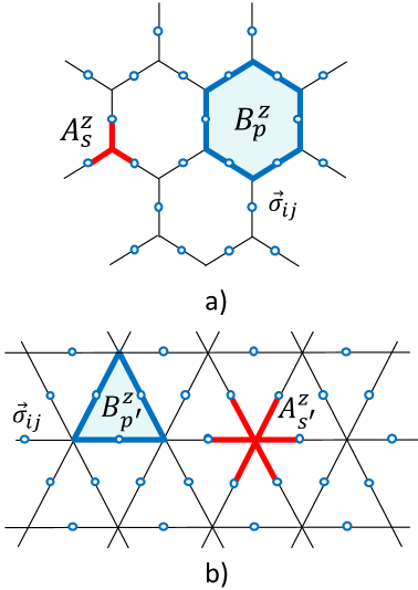
Figure 8: a) Hexagonal lattice and b) Triangular lattice. In panel a) the star terms $A^{z}_{s}$ and plaquette terms $B^{z}_{p}$ involve three and six spins $S$ (circles) interactions, respectively, while the opposite happens in panel b).

VIII Honeycomb and Triangular lattices

Thus far, we focused on square lattice realizations of the Ising, clock, and $U(1)$ theories. For completeness, we now examine other lattice geometries. Specifically, we study the honeycomb lattice (H) and triangular lattice (T) incarnations of our classical theory and determine their ground state degeneracies. In Fig. 8, $A^{z}_{s}$ and $B^{z}_{p}$ are defined for each lattice. The Hamiltonians are given by

$$H_{\sf H} = -J_{h}\sum_{s}A^{z}_{s}-J_{h}^{\prime}\sum_{p}B^{z}_{p},$$

$$H_{\sf T} = -J_{t}\sum_{s^{\prime}}A^{z}_{s^{\prime}}-J^{\prime}_{t}\sum_{p^{\prime}}B^{z}_{p^{\prime}}.$$ (59)

Our numerical results are summarized in Table 5. These results are consistent with Eqs. (46) and (49).

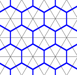
Figure 9: By connecting the centers of hexagons in an hexagonal lattice (thick solid lines), we obtain the corresponding dual lattice which is a triangular lattice (solid lines).

$g$	$E$	$D^{0}_{2}$	$D^{0}_{3}$	$D^{0}_{4}$	$D^{0}_{5}$	$D^{0}_{6}$	$D^{0}_{7}$	$D^{0}_{8}$	$D^{0}_{9}$
1	6	8	27	64	125	216	343	512	729
	12	16	27
	18	8
	24	128
2	24	128
	30	64

Table 5: Computed ground state degeneracy $D^{0}_{\sf M}$ for ${\sf d}_{Q}={\sf M}$, for a hexagonal lattice ($=$ triangular lattice).

As is well known, the H and T lattices are dual lattices (Fig. 9). This duality implies that the classical Toric Code models of Eq. (VIII) yield the same results. From Figs. 8 and 9, as a consequence of duality, what is defined as $A^{z}_{s}$ ($B^{z}_{p}$) in H corresponds to some $B^{z}_{p^{\prime}}$ ($A^{z}_{s^{\prime}}$) in T, and vice versa. This indicates that

$$A^{z}_{s} \overset{\sf Duality}{\longleftrightarrow} B^{z}_{p^{\prime}},$$

$$A^{z}_{s^{\prime}} \overset{\sf Duality}{\longleftrightarrow} B^{z}_{p}.$$ (60)

After this transformation we can rewrite Eqs. (VIII) as,

$$H_{\sf H} = -J_{h}\sum_{p^{\prime}}B^{z}_{p^{\prime}}-J_{h}^{\prime}\sum_{s^{\prime}}A^{z}_{s^{\prime}},$$

$$H_{\sf T} = -J_{t}\sum_{p}B^{z}_{p}-J^{\prime}_{t}\sum_{s}A^{z}_{s},$$ (61)

and assuming $J_{h}=J^{\prime}_{t},J_{h}^{\prime}=J_{t}$, it is seen that $H_{\sf H}=H_{\sf T}$. This simple analysis does not take into account potential boundary terms that may appear in finite lattices, as a result of the duality transformation.

IX Other classical models with holographic degeneracy

In this section, we dwell on a few more Ising type spin systems, similar to Type II commensurate lattice realizations of the classical Toric Code model (Eq. (27)), in which the degeneracy is holographic, i.e., exponential in the system’s boundary.

IX.1 Potts Compass Model

We now discuss a discretized version of the compass model Compass Model , the “$4$-state Potts compass model” on an $L_{x}\times L_{y}$ square lattice with periodic boundary conditions. The Hamiltonian is given by,

$$H_{\sf PC}=-\sum_{i,\sigma,\tau}\Big{(}n_{i\sigma}n_{i+\hat{x},\sigma}\sigma_{i}\sigma_{i+\hat{x}}+n_{i\tau}n_{i+\hat{y},\tau}\tau_{i}\tau_{i+\hat{y}}\Big{)},$$

where at each site (vertex) $i$ there are two Ising type spins $\sigma_{i}=\pm 1$, $\tau_{i}=\pm 1$, while the occupation numbers $n_{i\sigma}=0,1$ and $n_{i\tau}=1-n_{i\sigma}$. Then, at each site, there is either a $\sigma$ or a $\tau$ degree of freedom. The Cartesian unit vectors $\hat{x}$ and $\hat{y}$ link neighboring sites of the square lattice. Spins of the $\sigma$ type interact along the $x$-direction (horizontally) while those of the $\tau$ variety interact along the $y$-direction (vertically). Minimizing the energy is equivalent to maximizing the number of products in the summand of Eq. (IX.1) that are equal to $+1$. In a configuration in which at all sites there is a $\sigma$ (and no $\tau$) spin, the system effectively reduces to that of $L_{y}$ independent Ising chains parallel to the $x$ direction. For each such chain, there are two ground states: $\sigma_{i}=+1$ or $\sigma_{i}=-1$ for all lattice sites. As these chains are independent, there are $2^{L_{y}}$ ground states. Replacing some sites with $\tau$ spins some bonds turn into $0$ and energy increases as a result. Repeating the same procedure where all sites are occupied by $\tau$ spins, we find out that there are $L_{x}$ independent vertical Ising chains and so $2^{L_{x}}$ states giving the same minimum energy. The ground state degeneracy of Eq. (IX.1) is $2^{L_{x}}+2^{L_{y}}$. For a more general case with genus $g$ (composed of regions $\{a_{j}\}$ connected by bridges $\{b_{j}\}$ (shared by regions $a_{j}$ and $a_{j+1}$)), the degeneracy again depends on the number of independent horizontal ($L_{y}$) and vertical ($L_{x}$) Ising chains. If each region $a_{j}$ is of size $L^{j}_{x}\times L^{j}_{y}$ ($j=1,\cdots,g$) and $b_{j}$ ($j=1,\cdots,g-1$) is the number of edges connecting $a_{j}$ and $a_{j+1}$, then, the ground state degeneracy will be

$$n^{\sf Potts-compass}_{\sf g.s}=2^{L_{x}}+2^{L_{y}},$$ (63)

where

$$L_{x}=\sum^{g}_{j=1}L^{j}_{x}-\sum^{g-1}_{j=1}b_{j},~{}L_{y}=\sum^{g}_{j=1}L^{j}_{y}.$$ (64)

This degeneracy depends on both the geometry and the topology of the lattice. We briefly highlight the effects of topology in the degeneracy of Eqs. (63) and (64). Panel a) of Fig. 10 depicts a genus one lattice for which $L_{x}=5,L_{y}=12$ and $N=V=60$. By redefining the way spins are connected and boundary conditions, as we explained before, we may transform it into, e.g., $g=2,3$ lattices as in Fig. 10 (panels b) and c), respectively). Here, one may readily verify that although $L_{y}=12$ and the total number of spins do not change, $L_{x}$ varies (increases) as a result of increasing the genus number.

Figure 10: Three lattices with different genus numbers and their corresponding tori below. All have the same total number of spins, $N=60$. Thick solid (blue) lines represent the boundary and spins are located at the vertices. We have, a) $g=1$ and $L_{x}=5,L_{y}=12$. b) $g=2$ and $L_{x}=7,L_{y}=12$. c) $g=3$ and $L_{x}=9,L_{y}=12$.

IX.2 Classical Xu-Moore Model

As discussed earlier, our classical Toric Code model of Eq. (6) is identical to the spin (defined on vertices) plaquette model of Eq. (24). This latter Hamiltonian is, as it turns out, a particular limiting case of the so-called “Xu-Moore model” Xu-Moore1 ; Xu-Moore2 , one in which its transverse field is set to zero and the model becomes classical. In its original rendition, this classical limit of the Xu-Moore model has a degeneracy exponential in the system’s boundary. This degeneracy appears regardless of the parity of the system sides. We now discuss how to relate the degeneracy in our system to that of the classical Xu-Moore model. To achieve this, instead of applying periodic boundary conditions along the Cartesian directions as in the classical Toric Code model (i.e. along the solid lines of Fig. 2), we endow the system with different boundary conditions. Specifically, we examine instances in which periodic boundary conditions are associated with the diagonal $x^{\prime}$ and $y^{\prime}$ axis ($45^{\circ}$ angle rotation of the original square lattice) of Fig. 2. A simple calculation then illustrates that the ground state sector as well as all other energies have a global degeneracy factor,

$${\cal{N}}_{\sf global}=2^{L_{x^{\prime}}+L_{y^{\prime}}}.$$ (65)

where $L_{x^{\prime}}$ and $L_{y^{\prime}}$ are defined as in Eq. (64) but along the diagonal directions (dotted lines in Fig. 2). A similar (global) degeneracy appears in the classical 90^∘ orbital compass model kitaev_review (having only nearest neighbor two-spin interactions) to which the Xu-Moore model is dual.

IX.3 Second and Third nearest neighbor Ising models

We conclude our discussion of holographic degeneracy in spin models with a brief review of an Ising system even simpler than the ones discussed above. Specifically, we may consider an Ising spin system on a square lattice with its lattice constant $a$ set to unity when it is embedded on a torus ($g=1$) with periodic boundary conditions along the $x^{\prime}$ and $y^{\prime}$ diagonals with the Hamiltonian

$$H=\sum_{i,j}(2\delta_{|i-j|,\sqrt{2}}+\delta_{|i-j|,2})\sigma_{i}\sigma_{j}.$$ (66)

Here interactions are anti-ferromagnetic between next-nearest neighbors ($|i-j|=\sqrt{2}$) and next-next-nearest neighbors ($|i-j|=2$). It is straightforward to demonstrate that this system has a ground state degeneracy scales as $2^{L_{x^{\prime}}}+2^{L_{y^{\prime}}}$ where $L_{x^{\prime},y^{\prime}}$ are the lattice sizes along the $x^{\prime}$ and $y^{\prime}$ directions MW4 .

X Conclusions

In this work, we demonstrated that a topological ground state degeneracy (one depending on the genus number of the Riemann surface on which the lattice is embedded) does not imply concurrent topological order (i.e., Eq. (3) is violated and distinct ground states may be told apart by local measurements). We illustrated this by introducing the classical Toric Code model (Eq. (6) with $\mu=\nu=z$). As we showed in some detail, under rather mild conditions (those pertaining to “Type I” lattices in the classification of Eq. (27)), the ground state degeneracy solely depends on topology. In these classical systems, however, the ground states (given by, e.g., Eqs. (32) and (IV.3) on the torus) are distinguishable by measuring the pattern of $\sigma^{z}_{ij}$ on a finite number of nearest neighbor edges; thus, the ground states do not satisfy Eq. (3) and are, rather trivially, not topologically ordered. They are Landau ordered instead and, most importantly, illustrate that the ground states are related by $d=2$ (global) Gauge-like symmetries contrary to the $d=1$ symmetries of Kitaev’s Toric Code model symmetry1 ; symmetry2 ; fragility .

In the more commensurate Type II lattice realizations of the classical Toric Code model as well as in a host of other systems, the ground state degeneracy is “holographic”- i.e., exponential in the linear size of the lattice MW4 ; holography . This classical holographic effect is different from more subtle deeper quantum relations, for entanglement entropies, e.g., holo1 ; holo2 ; holo3 . In all lattices and topologies, the minimal ground state degeneracy (and that of all levels in the system) of the classical model is robust and bounded from below by $4^{g}$ with $g$ the genus number. We find similar genus dependent minimal degeneracies in clock and $U(1)$ theories (including lattice gauge theories). For completeness, we remark that a degeneracy of the form $2^{\eta(L)}$ with $\eta$ a quantity bounded from above by the linear system size (viz., a holographic entropy) also appears in bona fide topologically ordered systems such as the “Haah code” Haah ; Haah1 ; Haah2 .

Beyond demonstrating that such degeneracies may arise in classical theories, we illustrated that these behaviors may arise in rather canonical clock and $U(1)$ type theories. We provided a simple framework for studying and understanding the origin of these ubiquitous topological and holographic degeneracies.

We conclude with one last remark. Our results for classical systems enable the construction of simple quantum models with ground states that may be told apart locally (i.e., violating Eq. (3) for topological quantum order) yet, nevertheless, exhibit a topological ground state degeneracy). We present one, out of a large number of possible, routes to write such models exactly. Consider any one of the different theories studied in our work. Let us denote the classical Hamiltonian associated with any of these theories by $H_{\sf Classical}$ and corresponding local observables that may differentiate ground states apart by ${\cal V}$. One may then apply any product $U$ of local unitary transformations to both the Hamiltonian and the corresponding “order parameter” local observable ${\cal V}$. That is, we may consider the “quantum” Hamiltonian $H_{\sf Quantum}\equiv U^{\dagger}H_{\sf Classical}U$ and the corresponding local operator ${\cal V}_{\sf Quantum}\equiv U^{\dagger}{\cal V}U$. By virtue of the unitary transformation, both in the ground state sector (as well as at any finite temperature), the expectation value of the local observable ${\cal V}$ in the classical system given by $H_{\sf Classical}$ is identical to the expectation value of the ${\cal V}_{\sf Quantum}$ in the quantum system governed by $H_{\sf Quantum}$. To be concrete, one may consider, e.g., the Classical Toric Code (CTC) model. That is, e.g., one may set $H_{\sf Classical}=H_{\sf CTC}$ that contains only classical Ising ($\sigma^{x}_{j}$) spins. Next, consider the unitary operator $U=\prod_{j\in\Lambda_{+}}\exp[i\frac{\pi}{4}\sigma_{j}^{z}]$ that effects a $\pi/2$ rotation of all spins at sites $j$ that belong to the sublattice $\Lambda_{+}$ about the internal $\sigma^{z}$ axis. (That is, indeed, $\frac{1}{\sqrt{2}}(1-i\sigma_{j}^{z})\sigma_{j}^{x}\frac{1}{\sqrt{2}}(1+i\sigma_{j}^{z})=\sigma_{j}^{y}$.) Thus, trivially, the resulting Hamiltonian $H_{\sf Quantum}$ contains non-commuting $\sigma^{x}$ and $\sigma^{y}$ and is “quantum” (just as the Kitaev Toric Code model of Section III Fault-tolerant that may be mapped to two decoupled classical Ising spin chains symmetry1 ; symmetry2 ; fragility ) contains exactly these two quantum spin components and is “quantum”). By virtue of the local product nature of the mapping operator $U$, the classical local observables ${\cal V}$ that we discussed in our paper become now new local observables ${\cal V}_{\sf Quantum}$ in the quantum model. Thus, putting all of the pieces together, we may indeed generate quantum models with a topological degeneracy in which the ground state may be told apart by local measurements.

XI Acknowledgment

This work was partially supported by the National Science Foundation under NSF Grant No. DMR-1411229 and the Feinberg foundation visiting faculty program at the Weizmann Institute. We are very grateful to a discussion with J. Haah in which he explained to us the degeneracies found in his model Haah2 .

Appendix A Canonical Partition function of the Classical Toric Code Model

In Type I lattices (and their simplest composites), the canonical partition function of the classical Toric Code model is given by Eq. (36). The situation is somewhat richer for other lattices. Below, we briefly write the partition functions for several such finite size lattices. For simplicity we set $J=J^{\prime}=1$ and ${\sf d}_{Q}=2$ in the classical rendition of Eq. (6) and perform a high temperature (H-T) and low temperature (L-T) series expansion which is everywhere convergent for these finite size systems. One can follow a similar procedure and find the partition functions for ${\sf d}_{Q}>2$. We start with H-T series expansion,

$${\cal Z_{\sf H-T}} = \sum_{\{\sigma\}}e^{-\beta H^{z,z}}=\sum_{\{\sigma\}}e^{\beta\sum_{s}A^{z}_{s}+\beta\sum_{p}B^{z}_{p}}$$

$$= \sum_{\{\sigma\}}\prod_{s}e^{\beta A^{z}_{s}}\prod_{p}e^{\beta B^{z}_{p}}$$

$$= (\cosh\beta)^{V+F}\sum_{\{\sigma\}}\prod_{s}(1+T\,A^{z}_{s})\prod_{p}(1+T\,B^{z}_{p}),$$

where $T=\tanh\beta$ and $\beta=1/(k_{B}T)$.

In Eq. (A) after expanding the products, and summing over all configurations, the only surviving terms are those for which the product of a subset of $A^{z}_{s}$’s and $B^{z}_{p}$’s is equal to $1$ and this corresponds to one constraint or a product of two or more of them sharing no star or plaquette operators. Thus,

$${\cal Z_{\sf H-T}} = 2^{E}(\cosh\beta)^{V+F}$$

$$\times \Big{(}1+\text{terms from constraints on $A^{z}_{s}$'s and $B^{z}_{p}$'s}\Big{)},$$

where $F$ is the number of faces and $V$ is the number of vertices. The factor of $2^{E}$ (with $E=N$ the number of spins or lattice edges) originates from the summation $\sum_{\{\sigma\}}1$ (each $\sigma^{z}_{ij}$ has two values ($\pm 1$), with $(ij)=1,\cdots,E$). The sole non-vanishing traces in Eq. (A) originate from the constraints of Eqs. (IV.1) and (25) and their higher genus counterparts. While this procedure trivially gives rise to the partition function of Eq. (36) for simple lattices, the additional constraints in other lattices spawn new terms in the partition functions.

In the following we develop the L-T series expansion for ${\sf d}_{Q}=2$. From Eq. (36),

$${\cal Z_{\sf L-T}} = {\cal{N}}_{\sf global}\sum_{\ell=0}n_{\ell}e^{-\beta E_{\ell}}$$ (69)

$$= {\cal{N}}_{\sf global}e^{-\beta E_{0}}\Big{(}1+\sum_{\ell=1}n_{\ell}e^{-\beta(E_{\ell}-E_{0})}\Big{)},$$

where $E_{0}$ is the ground state energy and ${\cal{N}}_{\sf global}$ is the ground state degeneracy. Numerical results illustrate that the integers $n_{\ell}$ are larger than or equal to $1$. One can generalize this form for ${\sf d}_{Q}>2$

$${\cal Z_{\sf L-T}} = \sum_{\ell=0}D^{\ell}_{{\sf d}_{Q}}e^{-\beta E_{\ell}},$$ (70)

where $E_{\ell}$ and $D^{\ell}_{{\sf d}_{Q}}$ indicate energy and degeneracy of energy level $\ell$ for a given ${\sf d}_{Q}$, respectively.

Below is a sample of our numerical results for ${\cal Z}_{\sf H-T}$ and ${\cal Z}_{\sf L-T}$ of lattices with different sizes, ${\sf d}_{Q}$’s and genus numbers ($g=1,2,3$). From ${\cal Z}_{\sf L-T}$, we can easily see that exited states have a degeneracy “higher than or equal to” the ground state degeneracy ($J=J^{\prime}$ and $\beta J={\rm K}$).

1. $\bm{g=1}$:

   1. $\bm{3\times 1,E=6}$:

      1. ${\sf d}_{Q}=2$:

         $${\cal Z_{\sf H-T}} = (2\cosh\beta)^{6}\Big{(}1+T^{6}+2T^{3}\Big{)},$$

         $${\cal Z_{\sf L-T}} = 4(e^{6\text{K}})\Big{(}1+9e^{-8\text{K}}+6e^{-4\text{K}}\Big{)}.$$

      2. ${\sf d}_{Q}=3$:

         $${\cal Z_{\sf H-T}} = (3\cosh\beta)^{6}\Big{(}1+\frac{T^{6}}{32}+\frac{3T^{4}}{8}\Big{)},$$

         $${\cal Z_{\sf L-T}} = 9(e^{6\text{K}})\Big{(}1+10e^{-9\text{K}}+12e^{-\frac{15\text{K}}{2}}+36e^{-6\text{K}}$$

         $$+ 16e^{-\frac{9\text{K}}{2}}+6e^{-3\text{K}}\Big{)}.$$

      3. ${\sf d}_{Q}=4$:

         $${\cal Z_{\sf H-T}} = (4\cosh\beta)^{6}\Big{(}1+\frac{T^{6}}{16}\Big{)},$$

         $${\cal Z_{\sf L-T}} = 8(e^{6\text{K}})\Big{(}1+e^{-12\text{K}}+12e^{-10\text{K}}+135e^{-8\text{K}}$$

         $$+ 216e^{-6\text{K}}+135e^{-4\text{K}}+12e^{-2\text{K}}\Big{)}.$$

      4. ${\sf d}_{Q}=5$:

         $${\cal Z_{\sf H-T}} = (5\cosh\beta)^{6}\Big{(}1+\frac{T^{6}}{32}\Big{)},$$

         $${\cal Z_{\sf L-T}} = 5(e^{6\text{K}})\Big{(}1+90e^{\left(-\sqrt{5}-5\right)\text{K}}+90e^{\left(\sqrt{5}-5\right)\text{K}}$$

         $$+ 240e^{\left(\frac{1}{4}\left(-\sqrt{5}-1\right)+\sqrt{5}-6\right)\text{K}}+30e^{\left(\frac{1}{2}\left(-\sqrt{5}-1\right)-2\right)\text{K}}$$

         $$+ 210e^{\left(\frac{1}{2}\left(-\sqrt{5}-1\right)+\sqrt{5}-7\right)\text{K}}+12e^{\left(\frac{5}{4}\left(-\sqrt{5}-1\right)-5\right)\text{K}}$$

         $$+ 20e^{\left(\frac{3}{2}\left(-\sqrt{5}-1\right)-6\right)\text{K}}+240e^{\left(\frac{1}{4}\left(\sqrt{5}-1\right)-\sqrt{5}-6\right)\text{K}}$$

         $$+ 120e^{\left(\frac{1}{2}\left(-\sqrt{5}-1\right)+\frac{1}{4}\left(\sqrt{5}-1\right)-3\right)\text{K}}$$

         $$+ 120e^{\left(\frac{3}{4}\left(-\sqrt{5}-1\right)+\frac{1}{4}\left(\sqrt{5}-1\right)-4\right)\text{K}}$$

         $$+ 60e^{\left(\frac{5}{4}\left(-\sqrt{5}-1\right)+\frac{1}{4}\left(\sqrt{5}-1\right)-6\right)\text{K}}$$

         $$+ 30e^{\left(\frac{1}{2}\left(\sqrt{5}-1\right)-2\right)\text{K}}$$

         $$+ 210e^{\left(\frac{1}{2}\left(\sqrt{5}-1\right)-\sqrt{5}-7\right)\text{K}}$$

         $$+ 120e^{\left(\frac{1}{4}\left(-\sqrt{5}-1\right)+\frac{1}{2}\left(\sqrt{5}-1\right)-3\right)\text{K}}$$

         $$+ 360e^{\left(\frac{1}{2}\left(-\sqrt{5}-1\right)+\frac{1}{2}\left(\sqrt{5}-1\right)-4\right)\text{K}}$$

         $$+ 360e^{\left(\frac{3}{4}\left(-\sqrt{5}-1\right)+\frac{1}{2}\left(\sqrt{5}-1\right)-5\right)\text{K}}$$

         $$+ 120e^{\left(\frac{1}{4}\left(-\sqrt{5}-1\right)+\frac{3}{4}\left(\sqrt{5}-1\right)-4\right)\text{K}}$$

         $$+ 360e^{\left(\frac{1}{2}\left(-\sqrt{5}-1\right)+\frac{3}{4}\left(\sqrt{5}-1\right)-5\right)\text{K}}$$

         $$+ 240e^{\left(\frac{3}{4}\left(-\sqrt{5}-1\right)+\frac{3}{4}\left(\sqrt{5}-1\right)-6\right)\text{K}}$$

         $$+ 12e^{\left(\frac{5}{4}\left(\sqrt{5}-1\right)-5\right)\text{K}}$$

         $$+ 60e^{\left(\frac{1}{4}\left(-\sqrt{5}-1\right)+\frac{5}{4}\left(\sqrt{5}-1\right)-6\right)\text{K}}$$

         $$+ 20e^{\left(\frac{3}{2}\left(\sqrt{5}-1\right)-6\right)\text{K}}\Big{)}.$$

      5. ${\sf d}_{Q}=6$:

         $${\cal Z_{\sf H-T}} = (6\cosh\beta)^{6}\Big{(}1+\frac{T^{6}}{32}\Big{)},$$

         $${\cal Z_{\sf L-T}} = 36(e^{6\text{K}})\Big{(}1+6e^{-11\text{K}}+12e^{-10\text{K}}+24e^{-\frac{19\text{K}}{2}}$$

         $$+ 10e^{-9\text{K}}+48e^{-\frac{17\text{K}}{2}}+165e^{-8\text{K}}+12e^{-\frac{15\text{K}}{2}}$$

         $$+ 192e^{-7\text{K}}+168e^{-\frac{13\text{K}}{2}}+36e^{-6\text{K}}+96e^{-\frac{11\text{K}}{2}}$$

         $$+ 282e^{-5\text{K}}+16e^{-\frac{9\text{K}}{2}}+114e^{-4\text{K}}+60e^{-\frac{7\text{K}}{2}}$$

         $$+ 6e^{-3\text{K}}+24e^{-\frac{5\text{K}}{2}}+24e^{-2\text{K}}\Big{)}.$$

   2. $\bm{2\times 2,E=8}$:

      1. ${\sf d}_{Q}=2$:

         $${\cal Z_{\sf H-T}} = (2\cosh\beta)^{8}\Big{(}1+14T^{4}+T^{8}\Big{)},$$

         $${\cal Z_{\sf L-T}} = 16(e^{8\text{K}})\Big{(}1+e^{-16\text{K}}+14e^{-8\text{K}}\Big{)}.$$

      2. ${\sf d}_{Q}=3$:

         $${\cal Z_{\sf H-T}} = (3\cosh\beta)^{8}\Big{(}1+\frac{3T^{8}}{128}+\frac{T^{6}}{8}+\frac{3T^{4}}{4}\Big{)},$$

         $${\cal Z_{\sf L-T}} = 27(e^{8\text{K}})\Big{(}1+18e^{-12\text{K}}+16e^{-21\text{K}/2}$$

         $$+ 80e^{-9\text{K}}+64e^{-15\text{K}/2}+56e^{-6\text{K}}+8e^{-3\text{K}}\Big{)}.$$

      3. ${\sf d}_{Q}=4$:

         $${\cal Z_{\sf H-T}} = (4\cosh\beta)^{8}\Big{(}1+\frac{T^{8}}{16}+\frac{3T^{4}}{4}\Big{)},$$

         $${\cal Z_{\sf L-T}} = 128(e^{8\text{K}})\Big{(}1+e^{-16\text{K}}+44e^{-12\text{K}}+64e^{-10\text{K}}$$

         $$+ 294e^{-8\text{K}}+64e^{-6\text{K}}+44e^{-4\text{K}}\Big{)}.$$

   3. $\bm{4\times 1,E=8}$:

      1. ${\sf d}_{Q}=2$:

         $${\cal Z_{\sf H-T}} = (2\cosh\beta)^{8}\Big{(}1+2T^{4}+T^{8}\Big{)},$$

         $${\cal Z_{\sf L-T}} = 4(e^{8\text{K}})\Big{(}1+e^{-16\text{K}}+12e^{-12\text{K}}+38e^{-8\text{K}}$$

         $$+ 12e^{-4\text{K}}\Big{)}.$$

      2. ${\sf d}_{Q}=3$:

         $${\cal Z_{\sf H-T}} = (3\cosh\beta)^{8}\Big{(}1+\frac{T^{8}}{128}\Big{)},$$

         $${\cal Z_{\sf L-T}} = 3(e^{8\text{K}})\Big{(}1+86e^{-12\text{K}}+336e^{-\frac{21\text{K}}{2}}$$

         $$+ 616e^{-9\text{K}}+560e^{-\frac{15\text{K}}{2}}420e^{-6\text{K}}+112e^{-\frac{9\text{K}}{2}}$$

         $$+ 56e^{-3\text{K}}\Big{)}.$$

      3. ${\sf d}_{Q}=4$:

         $${\cal Z_{\sf H-T}} = (4\cosh\beta)^{8}\Big{(}1+\frac{T^{8}}{64}\Big{)},$$

         $${\cal Z_{\sf L-T}} = 16(e^{8\text{K}})\Big{(}1+e^{-16\text{K}}+8e^{-14\text{K}}+252e^{-12\text{K}}$$

         $$+ 952e^{-10\text{K}}+1670e^{-8\text{K}}+952e^{-6\text{K}}$$

         $$+ 252e^{-4\text{K}}+8e^{-2\text{K}}\Big{)}.$$

   4. $\bm{3\times 2,E=12}$:

      1. ${\sf d}_{Q}=2$:

         $${\cal Z_{\sf H-T}} = (2\cosh\beta)^{12}\Big{(}1+2T^{6}+T^{12}\Big{)},$$

         $${\cal Z_{\sf L-T}} = 4(e^{12\text{K}})\Big{(}1+e^{-24\text{K}}+30e^{-20\text{K}}$$

         $$+ 255e^{-16\text{K}}+452e^{-12\text{K}}+255e^{-8\text{K}}+30e^{-4\text{K}}\Big{)}.$$

      2. ${\sf d}_{Q}=3$:

         $${\cal Z_{\sf H-T}} = (3\cosh\beta)^{12}\Big{(}1+\frac{T^{12}}{2048}+\frac{3T^{8}}{128}\Big{)},$$

         $${\cal Z_{\sf L-T}} = 9(e^{12\text{K}})\Big{(}1+466e^{-18\text{K}}+2664e^{-\frac{33\text{K}}{2}}$$

         $$+ 7668e^{-15\text{K}}+12344e^{-\frac{27\text{K}}{2}}+14148e^{-12\text{K}}$$

         $$+ 11232e^{-\frac{21\text{K}}{2}}+6720e^{-9\text{K}}+2592e^{-\frac{15\text{K}}{2}}$$

         $$+ 1026e^{-6\text{K}}+152e^{-\frac{9\text{K}}{2}}+36e^{-3\text{K}}\Big{)}.$$

   5. $\bm{4\times 2,E=16}$:

      1. ${\sf d}_{Q}=2$:

         $${\cal Z_{\sf H-T}} = (2\cosh\beta)^{16}\Big{(}1+T^{16}+14T^{8}\Big{)},$$

         $${\cal Z_{\sf L-T}} = 16(e^{16\text{K}})\Big{(}1+e^{-32\text{K}}+8e^{-28\text{K}}+252e^{-24\text{K}}$$

         $$+ 952e^{-20\text{K}}+1670e^{-16\text{K}}+952e^{-12\text{K}}$$

         $$+ 252e^{-8\text{K}}+8e^{-4\text{K}}\Big{)}.$$

   6. $\bm{3\times 3,E=18}$:

      1. ${\sf d}_{Q}=2$:

         $${\cal Z_{\sf H-T}} = (2\cosh\beta)^{18}\Big{(}1+T^{18}+6T^{12}+9T^{10}$$

         $$+ 32T^{9}+9T^{8}+6T^{6}\Big{)},$$

         $${\cal Z_{\sf L-T}} = 64(e^{18\text{K}})\Big{(}1+9e^{-32\text{K}}+72e^{-28\text{K}}+636e^{-24\text{K}}$$

         $$+ 1296e^{-20\text{K}}+1422e^{-16\text{K}}+552e^{-12\text{K}}$$

         $$+ 108e^{-8\text{K}}\Big{)}.$$

2. $\bm{g=2}$

   1. $\bm{2\times 1+2\times 1,E=8}$:

      1. ${\sf d}_{Q}=2$:

         $${\cal Z_{\sf H-T}} = 2^{8}(\cosh\beta)^{6}\Big{(}1+T^{6}+T^{4}+T^{2}\Big{)},$$

         $${\cal Z_{\sf L-T}} = 16(e^{6\text{K}})\Big{(}1+e^{-12\text{K}}+7e^{-8\text{K}}+7e^{-4\text{K}}\Big{)}.$$

      2. ${\sf d}_{Q}=3$:

         $${\cal Z_{\sf H-T}} = 3^{8}(\cosh\beta)^{6}\Big{(}1+\frac{T^{6}}{32}\Big{)},$$

         $${\cal Z_{\sf L-T}} = 27(e^{6\text{K}})\Big{(}1+22e^{-9\text{K}}+60e^{-\frac{15\text{K}}{2}}$$

         $$+ 90e^{-6\text{K}}+40e^{-\frac{9\text{K}}{2}}+30e^{-3\text{K}}\Big{)}.$$

      3. ${\sf d}_{Q}=4$:

         $${\cal Z_{\sf H-T}} = 4^{8}(\cosh\beta)^{6}\Big{(}1+\frac{T^{6}}{16}\Big{)},$$

         $${\cal Z_{\sf L-T}} = 256(e^{6\text{K}})\Big{(}1+e^{-12\text{K}}+4e^{-10\text{K}}+71e^{-8\text{K}}$$

         $$+ 104e^{-6\text{K}}+71e^{-4\text{K}}+4e^{-2\text{K}}\Big{)}.$$

   2. $\bm{3\times 1+3\times 1(b_{1}=1),E=12}$:

      1. ${\sf d}_{Q}=2$:

         $${\cal Z_{\sf H-T}} = 2^{12}(\cosh\beta)^{10}\Big{(}1+T^{10}+T^{6}+T^{4}\Big{)},$$

         $${\cal Z_{\sf L-T}} = 16(e^{10\text{K}})\Big{(}1+e^{-20\text{K}}+21e^{-16\text{K}}$$

         $$+ 106e^{-12\text{K}}+106e^{-8\text{K}}+21e^{-4\text{K}}\Big{)}.$$

      2. ${\sf d}_{Q}=3$:

         $${\cal Z_{\sf H-T}} = 3^{12}(\cosh\beta)^{10}\Big{(}1+\frac{T^{10}}{512}+\frac{T^{7}}{32}+\frac{T^{6}}{32}\Big{)},$$

         $${\cal Z_{\sf L-T}} = 81(e^{10\text{K}})\Big{(}1+114e^{-15\text{K}}+572e^{-\frac{27\text{K}}{2}}+1266e^{-12\text{K}}$$

         $$+ 1716e^{-\frac{21\text{K}}{2}}+1530e^{-9\text{K}}+816e^{-\frac{15\text{K}}{2}}$$

         $$+ 438e^{-6\text{K}}+84e^{-\frac{9\text{K}}{2}}+24e^{-3\text{K}}\Big{)}.$$

   3. $\bm{3\times 1+3\times 1(b_{1}=2),E=12}$:

      1. ${\sf d}_{Q}=2$:

         $${\cal Z_{\sf H-T}} = 2^{12}(\cosh\beta)^{10}\Big{(}1+T^{10}+T^{6}+4T^{5}+T^{4}\Big{)},$$

         $${\cal Z_{\sf L-T}} = 32(e^{10\text{K}})\Big{(}1+13e^{-16\text{K}}+48e^{-12\text{K}}+58e^{-8\text{K}}$$

         $$+ 8e^{-4\text{K}}\Big{)}.$$

      2. ${\sf d}_{Q}=3$:

         $${\cal Z_{\sf H-T}} = 3^{12}(\cosh\beta)^{10}\Big{(}1+\frac{T^{10}}{512}+\frac{T^{7}}{32}+\frac{T^{6}}{32}\Big{)},$$

         $${\cal Z_{\sf L-T}} = 81(e^{10\text{K}})\Big{(}1+114e^{-15\text{K}}+572e^{-\frac{27\text{K}}{2}}+1266e^{-12\text{K}}$$

         $$+ 1716e^{-\frac{21\text{K}}{2}}+1530e^{-9\text{K}}+816e^{-\frac{15\text{K}}{2}}+438e^{-6\text{K}}$$

         $$+ 84e^{-\frac{9\text{K}}{2}}+24e^{-3\text{K}}\Big{)}.$$

   4. $\bm{2\times 2+2\times 1,E=12}$:

      1. ${\sf d}_{Q}=2$:

         $${\cal Z_{\sf H-T}} = 2^{12}(\cosh\beta)^{10}\Big{(}1+T^{10}+3T^{6}+3T^{4}\Big{)},$$

         $${\cal Z_{\sf L-T}} = 32(e^{10\text{K}})\Big{(}1+e^{-20\text{K}}+9e^{-16\text{K}}+54e^{-12\text{K}}$$

         $$+ 54e^{-8\text{K}}+9e^{-4\text{K}}\Big{)}.$$

      2. ${\sf d}_{Q}=3$:

         $${\cal Z_{\sf H-T}} = 3^{12}(\cosh\beta)^{10}\Big{(}1+\frac{T^{10}}{512}\Big{)},$$

         $${\cal Z_{\sf L-T}} = 27(e^{10\text{K}})\Big{(}1+342e^{-15\text{K}}+1700e^{-\frac{27\text{K}}{2}}$$

         $$+ 3870e^{-12\text{K}}+5040e^{-\frac{21\text{K}}{2}}+4620e^{-9\text{K}}$$

         $$+ 2520e^{-\frac{15\text{K}}{2}}+1260e^{-6\text{K}}+240e^{-\frac{9\text{K}}{2}}+90e^{-3\text{K}}\Big{)}.$$

3. $\bm{g=3}$:

   1. $\bm{2\times 1+2\times 1+2\times 1,E=12}$:

      1. ${\sf d}_{Q}=2$:

         $${\cal Z_{\sf H-T}} = 2^{12}(\cosh\beta)^{8}\Big{(}1+T^{8}+T^{6}+T^{2}\Big{)},$$

         $${\cal Z_{\sf L-T}} = 64(e^{8\text{K}})\Big{(}1+e^{-16\text{K}}+16e^{-12\text{K}}$$

         $$+ 30e^{-8\text{K}}+16e^{-4\text{K}}\Big{)}.$$

      2. ${\sf d}_{Q}=3$:

         $${\cal Z_{\sf H-T}} = 3^{12}(\cosh\beta)^{8}\Big{(}1+\frac{T^{8}}{128}\Big{)},$$

         $${\cal Z_{\sf L-T}} = 243(e^{8\text{K}})\Big{(}1+86e^{-12\text{K}}+336e^{-\frac{21\text{K}}{2}}+616e^{-9\text{K}}$$

         $$+ 560e^{-\frac{15\text{K}}{2}}+420e^{-6\text{K}}+112e^{-\frac{9\text{K}}{2}}+56e^{-3\text{K}}\Big{)}.$$

M

References

- (1) X.-G. Wen Quantum Field Theory of Many-Body Systems (Oxford University Press, Oxford, 2004).
- (2) For an explicit statement of the perceptive lore, see, e.g., page 8 of Wen for a remark concerning the quite deep standard manifestation of these degeneracies in the rich quantum arena: “The existence of topologically-degenerate ground states proves the existence of topological order. Topological degeneracy can also be used to perform fault-tolerant quantum computations (Kitaev, 2003).”
- (3) A. Yu. Kitaev, Ann. of Phys. 303, 2 (2003); arXiv:quant-ph/9707021 (1997).
- (4) B. Terhal, Rev. Mod. Phys. 87, 307 (2015).
- (5) J. Haah, Phys. Rev. A 83, 042330 (2011).
- (6) J. Haah, Comm. Math. Phys. 324(2), 351 (2013).
-
(7)
Specifically, on a cube of size endowed with
periodic boundary conditions, the degeneracy of Haah’s Code of
Haah ; Haah1 is equal to with set by the degree (in
) of the polynomial that constitutes the greatest common divisor of
the below three polynomials,
where . This degeneracy varies between and an exponential in and can exhibit capricious jumps as the lattice size is varied. For instance, (i) when (with a natural number) the degeneracy is while (ii) when , the degeneracy is four Haah ; Haah1 .(71) - (8) R. Peierls, Proc. Cambridge Phil. Soc. 32, 477 (1936); L. D. Landau and E. M. Lifshitz, Statistical Physics - Course of Theoretical Physics Vol 5 (Pergamon, London, 1958); J. Frolich, B. Simon, and T. Spencer, Commun. Math. Phys. 50, 79 (1976); R. Peierls, Contemporary Physics 33, 221 (1992).
- (9) L. D. Landau, Zh. Eksp. Teor. Fiz. 7, 19 (1937).
- (10) J. Bardeen, L. N. Cooper, and J. R. Schrieffer, Physical Review 106, 162 (1957).
- (11) V. L. Ginzburg and L. D. Landau, Zh. Eksp. Teor. Fiz. 20, 1064 (1950).
- (12) F. Wegner, J. Math. Phys. 12, 2259 (1971).
- (13) S. Elitzur Phys. Rev. D 12, 3978 (1975).
- (14) J. M. Kosterlitz and D. J. Thouless, Journal of Physics C: Solid State Physics 6, 1181 (1973); V. L. Berezinskii, Sov. Phys. JETP 32, 493 (1971).
- (15) N. D. Mermin and H. Wagner, Phys. Rev. Lett. 17, 1133 (1966).
- (16) P. C. Hohenberg, Phys. Rev. 158, 383 (1967).
- (17) S. Coleman, Commun. Math. Phys. 31: 259 (1973).
- (18) Z. Nussinov, arXiv:cond-mat/0105253 (2001).
- (19) D. C. Tsui, H. L. Stormer, and A. C. Gossard, Phys. Rev. Lett. 48, 1559 (1982).
- (20) R. B. Laughlin, Phys. Rev. Lett. 50, 1395 (1983).
- (21) E. Fradkin, Field Theories of Condensed Matter Physics, second Edition, (Cambridge University Press, Cambridge, 2013).
- (22) V. Kalmeyer and R. B. Laughlin, Phys. Rev. Lett. 59, 2095 (1987); V. Kalmeyer and R. B. Laughlin, Phys. Rev. B 39, 11879 (1989); X.-G. Wen, F. Wilczek, and A. Zee, Phys. Rev. B 39, 11413 (1989); H. Yao and S. A. Kivelson, Phys. Rev. Lett. 99, 247203 (2007); L. Messio, B. Bernu, and C. Lhuillier, Phys. Rev. Lett. 108, 207204 (2012); Yin-Chen He, D. N. Sheng, and Yan Chen, Phys. Rev. Lett. 112, 137202 (2014).
- (23) A. Yu. Kitaev, Ann. of Phys. 321, 2 (2006); arXiv:cond-mat/0506438 (2005).
- (24) Z. Nussinov and J. van den Brink, Rev. Mod. Phys. 87, 1 (2015); arXiv:1303.5922 (2013).
- (25) M. A. Levin and X.-G. Wen, Phys. Rev. B 71, 045110 (2005).
- (26) X.-G. Wen and Q. Niu, Phys. Rev. B 41, 9377 (1990).
- (27) X.-G. Wen, Phys. Rev. B 40, 7387 (1989).
- (28) X.-G. Wen, Int. J. Mod. Phys. B 4, 239 (1990).
- (29) G. Ortiz, Z. Nussinov, J. Dukelsky, and A. Seidel, Phys. Rev. B 88, 165303 (2013).
- (30) Y. Aharonov and D. Bohm, Phys. Rev. 115, 485 (1959).
- (31) M. Oshikawa and T. Senthil, Phys. Rev. Lett. 96, 060601 (2006).
- (32) E. Sagi, Y. Oreg, A. Stern, and B. I. Halperin, Phys. Rev. B 91, 245144 (2015).
- (33) E. Cobanera and G. Ortiz, Phys. Rev. A 89, 012328 (2014); Phys. Rev. A 91, 059901 (2015).
- (34) X.-G. Wen, Int. J. Mod. Phys. B 5, 1641 (1991).
- (35) Z. Nussinov and G. Ortiz, Ann. of Phys.(N.Y.) 324, 977 (2009); arXiv:cond-mat/0702377 (2007).
- (36) Z. Nussinov and G. Ortiz, Proceedings of the National Academy of Sciences, 106, 16944 (2009); arXiv:cond-mat/0605316 (2006).
- (37) Z. Nussinov and G. Ortiz, Phys. Rev. B 77, 064302 (2008).
- (38) In any particular fixed gauge, the degeneracy is (see, e.g., Eq. (187) of symmetry1 for a derivation). The factor of is the number of independent gauge fixes as can be seen as follows. The operators of Eq. (II) connect one gauge fix to another. There are such operators, and they are not independent of each other. Specifically, the local gauge symmetry operators adhere to the single global constraint of Eq. (12).
- (39) S. Mandal, R. Shankar, and G. Baskaran, J. Phys. A: Math. Theor. 45, 335304 (2012).
- (40) S. A. Kivelson, D. S. Rokhsar, and J. P. Sethna, Phys. Rev. B 35, 8865 (1987); D. S. Rokhsar and S. A. Kivelson, Phys. Rev. Lett. 61, 2376 (1988); R. Moessner and K. S. Raman, arXiv:0809.3051 (2008); F. S. Nogueira and Z. Nussinov, Physical Review B 80, 104413 (2009).
- (41) M. Sato, Phys. Rev. D 77, 045013 (2008).
- (42) T. H. Hansson, V. Oganesyan, and S. L. Sondhi, Annals of Physics 313, 497 (2004).
- (43) C. D. Batista and Z. Nussinov, Phys. Rev. B 72, 045137 (2005).
- (44) Z. Nussinov, G. Ortiz, and E. Cobanera, Annals of Physics 327, 2491 (2012).
- (45) D. Arovas, J. R. Schrieffer, and F. Wilczek, Phys. Rev. Lett. 53, 722 (1984).
- (46) S. B. Bravyi and A. Yu. Kitaev, arXiv:quant-ph/9811052 (1998).
- (47) N. Read and S. Sachdev, Phys. Rev. Lett. 66, 1773 (1991).
- (48) R. Moessner and S. L. Sondhi, Phys. Rev. Lett. 86, 1881 (2001).
- (49) G. Misguich, D. Serban, and V. Pasquier, Phys. Rev. Lett. 89, 137202 (2002).
- (50) L. Balents, M. P. A. Fisher, and S. M. Girvin, Phys. Rev. B 65, 224412 (2002).
- (51) O. I. Motrunich and T. Senthil, Phys. Rev. Lett. 89, 277004 (2002).
- (52) O. I. Motrunich, Phys. Rev. B 67, 115108 (2003).
- (53) M. Freedman, C. Nayak, K. Shtengel, K. Walker, and Z. Wang, Ann. Phys. (N.Y.) 310, 428 (2004).
- (54) C. Nayak, S. H. Simon, A. Stern, M. Freedman, and S. D. Sarma, Rev. Mod. Phys. 80, 1083 (2008).
- (55) J. Alicea, Reports on Progress in Physics 75, 076501 (2012).
- (56) X.-G. Wen, Int. J. Mod. Phys. B 6, 1711 (1992).
- (57) B. I. Halperin, Phys. Rev. B 25, 2185 (1982).
- (58) A. Kitaev and J. Preskill, Phys. Rev. Lett. 96, 110404 (2006); M. Levin and X. -G. Wen, Phys. Rev. Letts. 96, 110405 (2006).
- (59) C. D. Batista and G. Ortiz, Adv. in Phys. 53, 1 (2004).
- (60) E. Cobanera, G. Ortiz, and Z. Nussinov, Phys. Rev. B 87, 041105(R) (2013).
- (61) Apart from the models that we will introduce in the current paper, holographic degeneracies also appear in short range Ising, , non-Abelian gauge background, tiling holography ; MW4 ; glass ; langari ; klich , and other models. Indeed, holographic entropies have also been reported on fractal structures realized on lattices Moore1999 ; Yoshida .
- (62) Z. Nussinov, Phys. Rev. B 69, 014208 (2004).
- (63) M. Sadrzadeh and A. Langari, The European Physical Journal B 88, 259 (2015).
- (64) I. Klich, S. -H. Lee, and K. Iida Nature Communications 5, 3497 (2014).
- (65) M. E. J. Newman and C. Moore, Phys. Rev. E 60, 5068 (1999).
- (66) B. Yoshida, Phys. Rev. B 88, 125122 (2013); Ann. of Phys. 338, 134 (2013).
- (67) E. Cobanera, G. Ortiz, and Z. Nussinov, Phys. Rev. Lett. 104, 020402 (2010); E. Cobanera, G. Ortiz, and Z. Nussinov, Adv. in Phys. 60, 679 (2011); Z. Nussinov and G. Ortiz, Europhysics Letters 84, 36005 (2008); Z. Nussinov and G. Ortiz, Phys. Rev. B 79, 214440 (2009); G. Ortiz, E. Cobanera, and Z. Nussinov, Nuclear Physics B 854, 780 (2012).
- (68) R. Costa-Santos and B. M. McCoy, Nuclear Phys. B 623(3), 439 (2002).
- (69) Cenke Xu and J. E. Moore, Nucl. Phys. B 716, 487 (2005).
- (70) C. Xu and J. E. Moore, Phys. Rev. Lett. 93, 047003 (2004).
- (71) A, Mishra, M, Ma, F.-C. Zhang, S. Guertler, L.-H. Tang, and S. Wan. Phys. Rev. Lett. 93, 207201 (2004).
- (72) A. Pakman and A. Parnachev, JHEP 0807, 097 (2008).
- (73) S. Ryu and T. Takayanagi, Phys. Rev. Lett. 96, 181602 (2006).
- (74) L. McGough and H. Verlinde, JHEP 1311, 208 (2013).