Buckling and wrinkling from geometric and energetic viewpoints

Abstract

We discuss shape profiles emerging in inhomogeneous growth of squeezed tissues. Two approaches are used simultaneously: i) conformal embedding of two-dimensional domain with hyperbolic metrics into the plane, and ii) a pure energetic consideration based on the minimization of the total energy functional. In the latter case the non-uniformly pre-stressed plate, which models the inhomogeneous two-dimensional growth, is analyzed in linear regime under small stochastic perturbations. It is explicitly demonstrated that both approaches give consistent results for buckling profiles and reveal self-similar behavior. We speculate that fractal-like organization of growing squeezed structure has a far-reaching impact on understanding cell proliferation in various biological tissues.

I Introduction

Variety of shapes of growing objects emerges often due to incompatibility of internal growth protocol with geometrical restrictions imposed by embedding of growing substances into the space. For example, buckling of a salad leaf can be naively explained as a conflict between growth due to the reproduction of periphery cells, and geometrical growth of a circumference of a planar disc. It is known that there exists a biological mechanism which inhibits a cell growth if the cell experiences sufficient external pressure. So, cells located inside a body of growing tissue, preserve their size, while periphery cells have less steric restrictions an proliferate easier.

If the circumference, $P$, of a two-dimensional membrane (tissue) of typical radius $R$ grows faster than $P(R)\sim R$, one could expect buckling since ”extra material” goes out of plane and finds space in third dimension. The same is valid for growing 3D objects: suppose that growing surface, $S$, of a tissue (for example, a spherical cell colony of typical size $R$) grows faster than $S(R)\sim R^{2}$. In this case however, the expected colony shape is more cumbersome than for membranes, because the ”extra material” cannot go out in a forth dimension: our world is three-dimensional and the grows is accompanied by surface instabilities.

Certainly such naive geometric viewpoint does not take into account bending energy of deformed elastic tissues and definitely should be modified by an appropriate account of stresses existing in non-uniformly deformed elastic two– and three-dimensional objects. In this work, we restrict our consideration to growth of 2D objects only. Currently, two groups of works, devoted to the determination of shapes of growing bodies, can be distinguished in the literature.

In the first group of works, tentatively denoted as ”geometric” 1 ; 2 (see also 3 ), the determination of the typical profile of 2D surface is dictated by optimal ”isometric” embedding of discretized 2D surface into 3D space, and is described by an appropriate change of conformal metrics. This approach relies only on geometric constraints imposed by a ”conflict” between metric of a 3D Euclidean space and intrinsic hyperbolic metric of a 2D ideal membrane, and can be treated using the conformal methods. It should be mentioned, that formation of wrinkles within this approach seems to be closely related to description of phyllotaxis via conformal methods levitov . The discussion of possible connection between wrinkling patterns and energy relief of continuously deformed periodic 2D lattices of repulsive particles, will be considered separately.

In the second, more numerous group of works hebrew ; lewicka ; gemmer ; marder ; ignobel ; swinney , conventionally named ”energetic”, more realistic approach, based on minimization of a bending free energy of non-uniformly deformed thin elastic plates, is realized. Authors of almost all works, devoted to buckling of 2D growing tissues, state that ”geometric” and ”energetic” approaches are complimentary to each other. Besides, explicit comparison of results of these two approaches is still absent, as well as there is lack of analytic results obtained within the ”energetic approach”. In the current work we would like to fill this gap and consider from conformal (geometric) and energetic viewpoints wrinkling and buckling, paying attention to similarity and differences of obtained results.

The paper is organized as follows. In the Section II we discuss wrinkling in frameworks of a conformal approach and explicitly define the surface profile under the constraint of elementary surface area conservation. In Sections III-IV we consider buckling of non-uniformly squeezed thin plate obtained by minimization of its bending energy in linear approximation and summarize obtained results. Technical details of computations are presented in Appendices A-C.

II Conformal wrinkling

Surface wrinkling of constrained exponentially growing tissue can be tentatively described by the following naive geometric model. Consider initial flat elementary domain schematically depicted by the triangle $A$ in upper row of the Fig. 1a. Suppose that this domain represents, say, a linearly ordered colony of proliferating cells. If all cells divide independently and unconstrained, the colony doubles after some given time slot and expands its linear size.

To mimic the colony perimeter growth, suppose that 2nd generation of initial sample $A$ consists of two aligned copies of $A$. Repeating such duplication recursively, we arrive at a sequence of discrete time slots, $1,2,...k$, where in $k$th generation the perimeter of a colony, $P$, expressed in number of copies of $A$, is just $P(k)=2^{k-1}$. In absence of external confinement, two consequent duplications of initial sample $A$ are schematically shown in the Fig. 1a.

Now, to impose confinement effect which preserves the lateral size of a system, suppose that each generation $k$ of a colony, experiences lateral squeezing: as larger $P(k)$, as more external pressure should be applied to return the length of a colony, $P(k)$, to its initial size, $P(k=1)$, – as it is shown in the Fig. 1a. Under such a squeezing the elementary domains become essentially deformed: as larger $k$, as more compressed the elementary domains $A$ in a corresponding generation – see the Fig. 1b. Impose now an ”incompressibility condition” and demand the domains $A$ to preserve their surface areas in all generations. To satisfy this condition, the squeezed elementary domains should buckle in third dimension orthogonal to the plane of figures.

II.1 The model

Let us reformulate the above hand-waving viewpoint on buckling in more rigorous terms allowing analytic treatment. Make the nonuniform (exponential) discrete contraction of the sample shown in the Fig. 1c in vertical direction: the row $k$ is contracted by the factor $2^{k-1}$ along the $y$-axis. Such contraction together with above defined squeezing gives the ”discrete hyperbolic tessellation” of a domain shown in the Fig. 1c. The solid lines connecting the centers of neighboring triangles constitute the hyperbolic graph embedded into this domain.

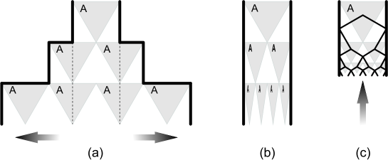
Figure 1: Nonuniform squeezing of a sample consisting of duplicating elementary cells $A$: a) Exponentially increasing lateral pressure is applied to each generation of samples $A$ to return them to initial size shown by dotted line; b) Schematic illustration of result of nonuniform (exponential) squeezing; c) Structure of a sample after nonuniform compression in vertical direction. The sample is covered by the hyperbolic regular lattice.

To make this hyperbolic tessellation consistent with the tessellation of Euclidean plane, we should proceed as it has been prescribed in 1 . Namely, take an equilateral triangle $A$ in the complex plane $z=x+iy$ with Euclidean metrics, $ds^{2}=dx^{2}+dy^{2}$, and make a conformal mapping of $A$ onto circular hyperbolic triangle $A^{\prime}$ with angles $\{\alpha,\alpha,0\}$ ($0\leq\alpha\leq\pi/3$) lying in the upper half-plane $\textrm{Im}\,w>0$ of the plane $w=u+iv$ endowed with the Hyperbolic metric $d\sigma^{2}=\frac{du^{2}+dv^{2}}{v^{2}}$. Let us denote this conformal mapping as $z(w)$. Below we provide an explicit construction of $z(w)$.

Other triangles in the Euclidean plain $z$ can be recursively obtained by reflections of the domain $A$ with respect to its sides, then – with respect to the sides of its images, etc. Correspondingly, we tessellate the Hyperbolic domain and cover isometrically the strip in the Fig. 2b by the images of the equilateral triangle $A$. Remind that isometric covering means that it preserves angles and distances in a given metrics.

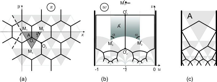
Figure 2: Conformal mapping of Euclidean complex plane $z=x+iy$ to the half-strip $v>0$ ($0\leq u\leq 1$) of the complex plane $w=u+iv$ with hyperbolic metrics. The mapping is defined by the conformal transform of the equilateral triangle $M_{1}M_{2}N_{3}$ (a) to the circular triangle $M_{1}^{\prime}M_{2}^{\prime}M_{3}^{\prime}$ with angles $\{\alpha,\alpha,0\}$ (b). The figure (b) is drawn for specific value $\alpha=\pi/3$. The figure (c) is the same as Fig. 1c and and is drawn to emphasize the similarity with discrete squeezing shown in the Fig. 1.

It is easy to check that the conformal mapping $z(w)$ preserves the area of the hyperbolic triangles. Namely, the area $S_{A}$ of the triangle $A$ in the the plane $z$ can be written as

$$S_{A}=\int\limits_{\triangle A}dxdy$$ (1)

where the integration is restricted by the boundary of the triangle. After the conformal mapping the area of the hyperbolic triangle $A^{\prime}$ should not be changed and therefore it reads

$$S_{A^{\prime}}=\int\limits_{\triangle A^{\prime}}|J(z,w)|dudv$$ (2)

where

$$J(z,w)=\left|\begin{array}[]{cc}\displaystyle\frac{\partial x}{\partial u}&\displaystyle\frac{\partial y}{\partial u}\;\vskip 6.0pt plus 2.0pt minus 2.0pt\\ \displaystyle\frac{\partial x}{\partial v}&\displaystyle\frac{\partial y}{\partial v}\end{array}\right|$$ (3)

is the Jacobian of conformal mapping $z(w)$. If $z(w)$ is holomorphic function, the Cauchy-Riemann conditions allow to express $J(w)$ as follows:

$$J(w)=\left|\frac{dz(w)}{dw}\right|^{2}$$ (4)

Let us connect the value of the Jacobian $J(w)$ at the point $w=u+iv$ with the surface height above the point $(u,v)$ in the plane $w$. Supposing that the surface is defined by the function $f(u,v)$, we have straightforwardly

$$J(w)=\sqrt{1+\left(\frac{\partial f}{\partial u}\right)^{2}+\left(\frac{\partial f}{\partial v}\right)^{2}}$$ (5)

Hence, the nonlinear partial differential equation

$$\left(\frac{\partial f(u,v)}{\partial u}\right)^{2}+\left(\frac{\partial f(u,v)}{\partial v}\right)^{2}=\left|\frac{dz(w)}{dw}\right|^{4}-1$$ (6)

where $z(w)$ is a known function, defines implicitly the height profile $f(u,v)$ of buckling surface above the plane $w$ tessellated by images of equilateral triangles. By changing $\alpha$ we can change the effective curvature and study the dependence of the profile on $\alpha$. However, note that the conformal approach is valid only for $0\leq\alpha\leq\pi/3$ and fails for $\alpha>\pi/3$. The function $f(u,v)$ is our desire, which should be later compared with the wrinkling profile of nonuniformly squeezed elastic membrane.

II.2 Construction of the conformal map $z(w)$

The conformal transform $z(w)$ which maps the triangle $M_{1}M_{2}M_{3}$ in $z$ onto the triangle $M_{1}^{\prime}M_{2}^{\prime}M_{3}^{\prime}$ in $w$ can be realized in two sequential steps as described in 1 ; 4 .

First of all, we map the triangle $M_{1}M_{2}M_{3}$ onto the upper half-plane of auxiliary complex plane $\zeta=\xi+i\eta$ with three branching points at 0, 1 and $\infty$. This mapping is realized by the function $z(\zeta)$:

$$z(\zeta)=\frac{1}{B\left(\frac{1}{3},\frac{1}{3}\right)}\int_{0}^{\zeta}\frac{d\zeta^{\prime}}{\zeta^{\prime 2/3}(1-\zeta^{\prime})^{2/3}}$$ (7)

where $B\left(\frac{1}{3},\frac{1}{3}\right)$ is the $\beta$-function. The correspondence of the branching points is as follows:

$$\begin{array}[]{lll}M_{1}(z=0)&\to&\tilde{M}_{1}(\zeta=0)\vskip 6.0pt plus 2.0pt minus 2.0pt\\ M_{2}(z=1)&\to&\tilde{M}_{1}(\zeta=1)\vskip 6.0pt plus 2.0pt minus 2.0pt\\ M_{3}\left(z=e^{-i\frac{\pi}{3}}\right)&\to&\tilde{M}_{3}(\zeta=\infty)\end{array}$$ (8)

Next step consists in mapping the auxiliary upper half-plane $\textrm{Im}\,\zeta>0$ onto the circular triangle $M^{\prime}_{1}M^{\prime}_{2}M^{\prime}_{3}$ with angles $\{\alpha,\alpha,0\}$ – the fundamental domain of the Hecke group in $w$. This mapping is realized by the function $\zeta(w)$, which can be constructed as follows koppenfels . Let $w(\zeta)$ be the inverse function of $\zeta(w)$ and represent it as a quotient

$$w(\zeta)=\frac{\phi_{1}(\zeta)}{\phi_{2}(\zeta)}$$ (9)

where $\phi_{1,2}(\zeta)$ are the fundamental solutions of the 2nd order differential equation of Picard-Fuchs type:

$$\zeta(\zeta-1)\phi^{\prime\prime}(\zeta)+\left(\left(a+b+1\right)\zeta-c\right)\phi^{\prime}(\zeta)+ab\phi(\zeta)=0$$ (10)

It is known caratheodory ; koppenfels that the function $w(\zeta)$ conformally maps the generic circular triangle with angles $\{\alpha_{0},\alpha_{1},\alpha_{\infty}\}$ in the upper halfplane of $w$ onto the upper halfplane of $\zeta$ with the following correspondence of points:

$$\left\{\begin{array}[]{ll}\mbox{In vertex $w(\zeta=0)$}&\mbox{angle $\alpha_{0}=\pi|c-1|$}\vskip 6.0pt plus 2.0pt minus 2.0pt\\ \mbox{In vertex $w(\zeta=1)$}&\mbox{angle $\alpha_{1}=\pi|a+b-c|$}\vskip 6.0pt plus 2.0pt minus 2.0pt\\ \mbox{In vertex $w(\zeta=\infty)$}&\mbox{angle $\alpha_{\infty}=\pi|a-b|$}\end{array}\right.$$ (11)

Choosing $\alpha_{\infty}=0$ and $\alpha_{0}=\alpha_{1}=\alpha$, we can express the parameters $(a,b,c)$ of the equation (10) in terms of $\alpha$, taking into account that the triangle $M_{1}^{\prime}M_{2}^{\prime}M_{3}^{\prime}$ in the Fig. 2b is parameterized as follows $\{\alpha_{0},\alpha_{1},\alpha_{\infty}\}=\{\alpha,\alpha,0\}$:

$$a=b=\frac{\alpha}{\pi}+\frac{1}{2},\quad c=\frac{\alpha}{\pi}+1$$ (12)

This leads us to the following particular form of equation (10)

$$\zeta(\zeta-1)\phi^{\prime\prime}(\zeta)+\left(\frac{\alpha}{\pi}+1\right)(2\zeta-1)\phi^{\prime}(\zeta)+\left(\frac{\alpha}{\pi}+\frac{1}{2}\right)^{2}\phi(\zeta)=0$$ (13)

where $\alpha=\frac{\pi}{m}$ and $m=3,4,...\infty$. For $\alpha=0$ Eq.(13) takes especially simple form, known as Legendre hypergeometric equation,

$$\zeta(\zeta-1)\phi^{\prime\prime}(\zeta)+(2\zeta-1)\phi^{\prime}(\zeta)+\frac{1}{4}\phi(\zeta)=0$$ (14)

The pair of possible fundamental solutions of (14) reads

$$\begin{array}[]{l}\phi_{1}(\zeta)=F\left(\frac{1}{2},\frac{1}{2},1,\zeta\right);\vskip 6.0pt plus 2.0pt minus 2.0pt\\ \phi_{2}(\zeta)=iF\left(\frac{1}{2},\frac{1}{2},1,1-\zeta\right)\end{array}$$ (15)

Substituting (15) into (9) we get $w(\zeta)$. The inverse function $\zeta(w)$ is the so-called modular function, $k^{2}(w)$ (see modular for details), i.e.

$$\zeta(w)\equiv k^{2}(w)=\frac{\theta_{2}^{4}(0,e^{i\pi w})}{\theta_{3}^{4}(0,e^{i\pi w})}$$ (16)

where $\theta_{2}$ and $\theta_{3}$ are the elliptic Jacobi $\theta$-functions jacobi . The correspondence of branching points for the auxiliary mapping $\zeta(w)$ is as follows:

$$\begin{array}[]{lll}\tilde{M}_{1}(\zeta=0)&\to&M^{\prime}_{1}(w=\infty)\vskip 6.0pt plus 2.0pt minus 2.0pt\\ \tilde{M}_{2}(\zeta=1)&\to&M^{\prime}_{1}(w=0)\vskip 6.0pt plus 2.0pt minus 2.0pt\\ \tilde{M}_{3}(\zeta=\infty)&\to&M^{\prime}_{3}(w=-1)\end{array}$$ (17)

Collecting (7) and (16) we arrive at an explicit expression for a composite map, $z(\zeta(w))$. Computing the Jacobian (4) of this composite conformal mapping, we get

$$J(w)\equiv\left|\frac{dz(w)}{dw}\right|^{2}=\frac{\left|\eta(w)\right|^{8}}{\pi^{2/3}B^{2}(\frac{1}{3},\frac{1}{3})}$$ (18)

where

$$\eta(w)=e^{\pi iw/12}\prod_{n=0}^{\infty}(1-e^{2\pi inw})\quad(w=u+iv)$$ (19)

is $\eta(w)$ the Dedekind $\eta$-function jacobi .

The profile $f(u,v)$ of the surface wrinkling above the plane $w=u+iv$ can be computed now from the Eq.(6), which for the particular choice of the Jacobian $J(w)$, defined by (18), reads

$$\left(\frac{\partial f(u,v)}{\partial u}\right)^{2}+\left(\frac{\partial f(u,v)}{\partial v}\right)^{2}=\frac{\left|\eta(w)\right|^{16}}{\pi^{4/3}B^{4}(\frac{1}{3},\frac{1}{3})}-1$$ (20)

It is worth mentioning that (20) has a form of eminent eikonal equation for wave propagation time to the point $(x,y)$ in the medium that allows for a certain wave speed $c(x,y)$, namely $|\nabla T(x,y)|^{2}=\frac{1}{c(x,y)}$ with the source initially located at some surface $\Gamma$, with initial Dirichlet conditions geo1 ; geo2 . Solving numerically (20), we get the surface profile $f(u,v)$, shown in the Fig. 3 (left).

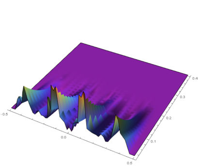
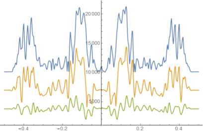
Figure 3: Numerical solution of the eikonal equation (20) for buckling surface in the geometrical approach (left). Few solutions for the free edge profile in the geometrical approach for $v=0.07,0.05,0.03$ (right).

Buckling profile near the open boundary $v=0$, for exponential growth of cells is shown in the Fig. 3 (right) for few values $v=0.07,0.05,0.03$. Later on we shall compare these profiles with the ones derived via energetic approach. Note that with progression towards the free edge (i.e. for $v\to 0$), the shape develops novel peaks vegetating from previous ones. It will be shown later that the same structure emerges in growth considered in the frameworks of energetic approach.

III Energetic approach to buckling

Here we discuss continuous energetic model of a shape formation in a very thin planar elastic tissue growing between two impenetrable walls. We conjecture that this model mimics growth in the situation when cell division works homogeneously with a certain time-dependent rate about the whole width of the sample squeezed between the walls. Specifically, the growth rate is chosen such that cell density is gradually increasing towards the direction of growth. Buckling of plants leaves contribute to the belief, that there exists some correlation length, on which tissue benefits from local breaking of planar topology, which occurs as a sort of bifurcation and is a fundamental biological and physical property.

The cell division rate is crucial for resulting profiles, giving rise a variety of buckling forms and shapes in different biological systems. We put this parameter in our model as the number of cells, $N(y)$, in a layer $y$, where $y\equiv y(t)$ characterizes the kinetics of cell division. The advantage of elastic approach consists in the possibility to develop sufficiently simple general solution for the stable shape of elastic tissue from the system energy minimization. This approach can be extended to the model which takes into account random inhomogeneity in growth rate and in boundary conditions.

The model of the nonuniformly squeezed elastic tissue is set as follows. Consider a 2D sample grown till time $t$, that buckles out of its plane since it has to grow under the constraints imposed by walls, that prevent increasing of the in-plane sample width. If we now let the grown tissue to relax, the tissue will loose its buckling profile and adopt a smooth, not deformed one, as depicted in the Fig. 4. As long as this resulting state can be taken for the reference one, and we believe there is no energy loss during the relaxation, the work needed to keep walls is equal to buckling deformation energy. On next step, we may recreate buckling picture by applying certain forces to the walls. Eventually, buckling at time $t$ obtained by grown 2D tissue can be understood in terms of the model of the plate with some sort of gradual prestress applied. Since we consider linear regime only, there is no in-plane deformations before the plate starts buckling out. Thus this prestress does not change the size of the plate and the contour length of each row is conserved as we move from relaxed state to the prestressed one.

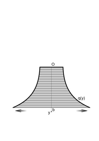
Figure 4: Relaxed tissue when two walls have been taken away.

Now let us take a closer look on a prestressed plate a thickness $h(a,b\gg h)$ that undergoes compressing contour forces $q(y)$ distributed along the edges $x=-a/2$ and $x=a/2$, that are kept fixed. The growth spreads in $y$ direction and the side of the plate $y=0$, where the growing starts, is fixed also. The question we will be interested in, is which buckling should minimize the full energy of the system grown under such conditions? It is known that the energy of in-plane strain scales as $H_{in}\sim h$ while the energy of out-plane ”buckling-kind” deformations scales as $H_{out}\sim h^{3}$, which implies that thin enough plates would benefit from buckling instead of staying stable. It will be shown further that buckling complexity crucially depends on the thickness.

In tense state the full energy, $H$, is the sum of deformation energy, $U$, and of its potential counterpart of applied forces, $P$, i.e. $H=U+P$. By minimizing the energy functional, the equation on equilibrium buckling profile can be obtained. The main steps of the derivation are presented here, while more elaborated description constitutes the subject of the Appendix A.

In linear approximation the deformation energy of an elastic sample can be written in terms of tension and deformation tensor components:

$$U=\frac{1}{2}\int\limits_{V}\bigg{(}\sum_{i}\sigma_{i}\epsilon_{i}+\sum_{i\neq j}\tau_{ij}\gamma_{ij}\bigg{)}dV$$ (21)

where $i=\{x,y,z\},j=\{x,y,z\}$, $i\neq j$, and $\tau_{ij}=\tau_{ji}$, $\gamma_{ij}=\gamma_{ji}$.

The potential energy of applied forces is measured by the work needed to get from this state to the reference one which is regarded as an unbuckling state.

$$P=\int\limits_{-a/2}^{a/2}\int\limits_{0}^{b}q(y)\left[w\partial^{2}_{xx}w+\left(\partial_{x}w\right)^{2}\right]dxdy,$$ (22)

Minimizing the resulting energy functional, we get the Euler equation for the equilibrium shape $w(x,y)$

$$D\Delta^{2}w(x,y)+P=0$$ (23)

where $D=\frac{Eh^{3}}{12(1-\mu^{2})}$ is bending stiffness of a plate, $P=3q(y)\frac{\partial^{2}w}{\partial x^{2}}$, and $\Delta=\partial_{xx}^{2}+\partial_{yy}^{2}$.

Equation (23) is a linear form of the well-known Föppl-von-Karman (FvK) equation muller ; lewicka ; gemmer for out-of-plane displacement of a thin homogeneous rectangular plate. It can give us some insight on the eigenfunctions of the plate, however due to its linear structure, (23) can say nothing neither about dynamics of the system on the phase plane ”force-harmonics” between different bifurcation points, nor about the types of these bifurcations. The nonlinear parts should be analyzed to understand the process deeper. However external errors, for example at the boundaries, can increase the number of intersections of different trajectories on the phase plane and effectively smear some of nonlinear peculiarities. As a result, the system may exist in many eigenstates at the same time and the problem of choosing between different states becomes purely statistical.

To simplify forthcoming espressions, rewrite (23) as:

$$D\left(\partial^{4}_{xxxx}w+2\partial^{4}_{xxyy}w+\partial^{4}_{yyyy}w\right)+q(y)\partial^{2}_{xx}w=0$$ (24)

where the reassignment $q\to 3q$ is made.

Note that in the limit of infinite growing times and constant compressing force, we arrive at the Euler equation for rod bending. The solution for eigenfunctions takes the well-known form, $w_{n}(x)=A_{n}\sin\frac{n\pi x}{a}$, where $q_{n}=\frac{n^{2}\pi^{2}D}{a}$ are the eigenvalues of corresponding Sturm-Liouville problem.

Our growth model implies that the plate is fixed on three sides, namely at $x=-\frac{a}{2}$, $x=\frac{a}{2}$ and $y=0$, where the $z$-displacement, $w(x,y)$ nullifies. Moreover deformations nullify as well since our plate can freely rotate at the boundaries. At forth open edge (the surface) both, tension and forces, vanish (see Appendix B for details):

$$\left\{\begin{array}[]{r}w\left(-\frac{a}{2},y\right)=\partial^{2}_{xx}w\left(-\frac{a}{2},y\right)=0\vskip 6.0pt plus 2.0pt minus 2.0pt\\ w\left(\frac{a}{2},y\right)=\partial^{2}_{xx}w\left(\frac{a}{2},y\right)=0\vskip 6.0pt plus 2.0pt minus 2.0pt\\ w(x,0)=\partial^{2}_{yy}w(x,0)=0\vskip 6.0pt plus 2.0pt minus 2.0pt\\ \partial^{2}_{yy}w(x,b)+\mu\partial^{2}_{xx}w(x,b)=0\vskip 6.0pt plus 2.0pt minus 2.0pt\\ \partial^{3}_{xxx}w(x,b)+(2-\mu)\partial^{3}_{xxy}w(x,b)=0\end{array}\right.$$ (25)

The symmetry of the problem forces the solution to be even or odd in $x$ coordinate (relatively to the center of the plate). Thus, we seek the solution in terms of sine- or cosine-Fourier series in $x$. The resulting coefficients are weighted functions of $y$. To satisfy boundary conditions at $x=\frac{a}{2}$ and $x=-\frac{a}{2}$, one should require the sine series to be over only even harmonics and the cosine series - over odd harmonics:

$$\begin{array}[]{l}\displaystyle w_{S}(x,y)=\sum_{n=0}^{\infty}Y_{n}(y)\sin\frac{2\pi nx}{a}\vskip 6.0pt plus 2.0pt minus 2.0pt\\ \displaystyle w_{C}(x,y)=\sum_{n=0}^{\infty}Y_{n}(y)\cos\frac{(2n+1)\pi x}{a}\end{array}$$ (26)

Substituting (26) in (24), we get the following fourth-order equation for $Y_{n}(y)$:

$$\partial^{4}_{yyyy}Y_{n}(y)-2S_{n}\partial^{2}_{yy}Y_{n}(y)+S_{n}\left(S_{n}-\frac{q(y)}{D}\right)Y_{n}(y)=0$$ (27)

where

$$S_{n}=\left\{\begin{array}[]{ll}\left(\frac{2n\pi}{a}\right)^{2}&\mbox{for sine-solutions}\vskip 6.0pt plus 2.0pt minus 2.0pt\\ \left(\frac{(2n+1)\pi}{a}\right)^{2}&\mbox{for cosine-solutions}\end{array}\right.$$ (28)

Equations (27)-(28) are equipped with the following boundary conditions:

$$\left\{\begin{array}[]{r}Y_{n}(0)=\partial^{2}_{yy}Y_{n}(0)=0\vskip 6.0pt plus 2.0pt minus 2.0pt\\ \partial^{2}_{yy}Y_{n}(b)-\mu S_{n}Y_{n}(b)=0\vskip 6.0pt plus 2.0pt minus 2.0pt\\ \partial^{3}_{yyy}Y_{n}(b)-(2-\mu)S_{n}\partial_{y}Y_{n}(b)=0\end{array}\right.$$ (29)

The Sturm-Liouville problem (27)-(29) cannot be solved analytically for generic squeezing protocol $q$, however can be treated exactly for $q(y)=q={\rm const}$, since in that case it becomes a linear differential equation with constant coefficients. The solution for $q(y)=q$ reads

$$Y_{n}(y)=A_{1}\sin\alpha_{n}y+A_{2}\cos\alpha_{n}y\\ +A_{3}\sinh\beta_{n}y+A_{4}\cosh\beta_{n}y,$$ (30)

where

$$\alpha_{n}=\sqrt{S_{n}}\sqrt{-1+\sqrt{\frac{q}{D}S_{n}}};\quad\beta_{n}=\sqrt{S_{n}}\sqrt{1+\sqrt{\frac{q}{D}S_{n}}}$$ (31)

Taking into account boundary conditions (29), we obtain:

• The amplitude,

  $$Y_{n}(y)\sim\sinh\beta_{n}y+\frac{\beta_{n}^{2}-\mu S_{n}}{\alpha_{n}^{2}+\mu S_{n}}\frac{\sinh\beta_{n}b}{\sin\alpha_{n}b}\sin\alpha_{n}y$$ (32)

• The spectral equation, which eventually determines the plate buckling modes,

  $$\frac{\alpha_{n}}{\beta_{n}}\tanh{\beta_{n}b}\cot{\alpha_{n}b}\frac{\beta_{n}^{2}-\mu S_{n}}{\alpha_{n}^{2}+\mu S_{n}}\frac{\alpha_{n}^{2}-(2-\mu)S_{n}}{\beta_{n}^{2}-(2-\mu)S_{n}}=1$$ (33)

Eq.(33) allows to determine harmonics, $n$. It can be inferred from the Fig. 5a that when the effective compressing parameter $\frac{q}{D}$ is small enough, only few harmonics are available in the plate. By increasing $\frac{q}{D}$ we increase number of possible harmonics, as shown in the Fig. 5b. Let us argue that in any real physical system, the unavoidable presence of noise makes the buckling ”uncertain”, meaning simultaneous presence of many harmonics, corresponding to the solution of (33). Indeed, suppose that due to fluctuations in initial conditions, the solution of (33) is known with some accuracy, $\epsilon$, designated in the Fig. 5a,b by the grey strip of width $\epsilon$. If $\epsilon$ is smaller than spacing between harmonics, only one solution is realized as shown in the Fig. 5a. Otherwise, one could have many solutions inside the strip of width $\epsilon$ – see Fig. 5b.

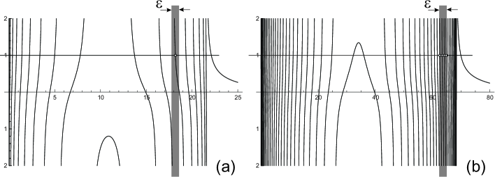
Figure 5: Graphic solution of (33) for the plate with $a=5$, $b=2$ and (a) $\frac{q}{D}=100$; (b) $\frac{q}{D}=1000$.

As approved by Fig. 5b, for soft enough surfaces buckling is mostly pronounced and the spectrum should be extremely dense. In this case, the gap between the energies of neighbouring harmonics (local minimizers) is much less the energy perturbations, induced by the errors. As long so, one can imply that the system lives in all the states at one time. In other words, the probabilities of the each eigenvector is the same. This allows to take all the weight functions in Fourier series with equal absolute amplitudes. But still the sign of the each wave amplitude is a subject that provides this problem with stochastic nature, because states that differ only by a sign have equal probabilities to survive.

We plot the squared buckling profile at the free edge, $w^{2}(x,b)$, in Fig. 6 for even and odd solutions. Interestingly, the profiles seem very similar, being different in small details only, such as a peak in the center. It can be seen from the Fig. 6, that constant compressing protocol gives homogeneous buckling with no fractal structure pronounced at the free edge. Nevertheless, homogenous squeezing is still of great importance since it gives us physical insight on the spectrum properties of the deformed plate.

Now we are going to proceed with numerical approach for non-constant $q(y)$ looking for fractal behavior. It has to be mentioned that in our approach we deal only with thin plates. It is well justified because all interesting features, such as intense buckling and fractal profiles, can be found only in soft enough systems, which means low values of bending stiffness, $D$. Thus having the thickness increased and jumping to 3D problem we leave little chances for buckling, according to spectral equation (33).

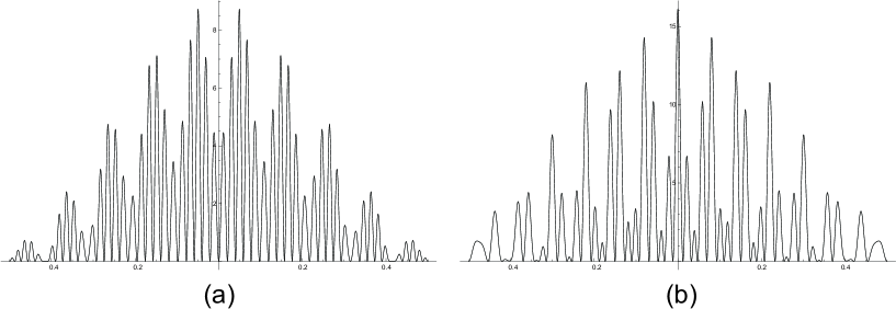
Figure 6: (a) Even and (b) odd buckling profiles for plates with $a=5$, $b=2$ and $\frac{q}{D}=10^{3}$.

IV Numerical solution of linear problem

For nonconstant squeezing protocol, $q(y)$, one solves (27) numerically for various modes $n$ and receive the $y$-dependent amplitudes for each harmonics. To proceed, replace each derivative in (27) by its finite-difference analog and convert it along with the boundary conditions (29) into the system of linear equations for the vector $u$:

$$A_{N}{\bf u}={\bf b},$$ (34)

where $N$ is the number of steps in the finite-difference scheme that divides the mattress length $a$ in equal step sizes $h=a/N$.

The matrix $A_{N}$ is five-diagonal and approximates the equation (27) with the accuracy $O(h^{2})$. Details of the derivations approximations and the explicit forms of matrix elements can be found in Appendix C. According to (27)-(29), the row ${\bf b}$ should be a null vector. In this case, we get only trivial solution ${\bf u}=0$ for any nonsingular $A_{N}$. It is well justified that semi-analytical spectral condition for non-constant compressing, analogous to (33), is

$$\det A_{N}(n)=0$$ (35)

for any large $N$.

Unfortunately, Eq.(35) is difficult to analyze due to general computational reasons, like increasing errors for sufficiently small step sizes, $h$. However, in linear regime one can legally find order of magnitude of critical forces $q(y)$ when first bucking appears. It is worth noting that the spontaneous symmetry breaking at the first buckling point, crucially depends on noise at boundaries of the plate and fluctuations in the bulk. Thus, in order to describe buckling profile we treat $b$ as a noise of small amplitude. Fluctuations in the lattice give rise to random matrices implementation. On this way one can improve (34) and write $M_{N}=A_{N}+R_{N}$, where $A_{N}$ is the matrix described above and $R_{N}$ is a random $N\times N$ matrix describing the perturbation. Then improved solution of (34) takes the following form:

$${\bf u}={\bf u}_{A}+\sum{\bf u}_{i}P(R_{i}),$$ (36)

where ${\bf u}_{A}$ is not perturbed solution with the matrix $A$, and ${\bf u}_{i}$ is the ”random solution” with the matrix $R_{i}$ such that $R_{i}{\bf u}_{i}={\bf b}$, and $P(R_{i})$ is the probability of the fluctuation $R_{i}$.

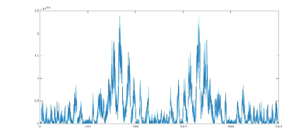
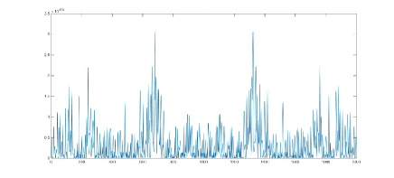
Figure 7: (left) Even buckling profile $w^{2}(x,b)$ on the free edge for the plate with $a=5$, $b=1$ for $q(y)\sim e^{y}$; (right) Odd buckling profile $w^{2}(x,b)$ on the free edge for the plate with $a=10$, $b=1$ for $q(y)\sim e^{y}$.

Discussion of specific properties of random matrices $R$ goes beyond the scopes of this work. We assume that it is possible to account for noise taking ${\bf b}$ as small random perturbation. First and last two elements of ${\bf b}$ describe noise at edges and other elements are responsible for fluctuations in the bulk of the plate. Solving (34) numerically with such choice of ${\bf b}$, one finds typical buckling profiles.

Let us now look on odd and even profiles on the free edge for exponential compressing protocol $q(y)\sim e^{y}$ Fig. 7. First, it can be noticed that at the center of the plate the fractal behavior qualitatively does not change. It was found that for larger $\frac{a}{b}$ new higher modes develop in the plate whose relative disposition mimics the picture at low $\frac{a}{b}$ and positions of peaks on subsequent hierarchical levels. These pictures were found stable to errors induced by the boundaries, especially at the central part of the plate. These profiles have striking similarities with the profiles derived via geometric approach, Fig. 3. Interestingly, no such self-similarity profiles have been found for other types of compressing protocol, $q(y)$, including the case of constant squeezing.

To show the effect of developing branching on the buckling surface with progression of $y$ towards the free edge, we have plotted the squared profiles, $w(x,y)$ on $x$ for different $y$, starting from $y=0$, see Fig. 8. Developing of new peaks as a result of fission of the previous ones is consistent with the model of cell division, as long as we used exponential squeezing protocol $q(y)$ in our computations.

V Conclusion

In this paper, using geometrical and energetic approaches, we have investigated equilibrium shapes of exponentially growing 2D patterns squeezed between plate boundaries. The resulting profiles posses self-similar organization, one of most crucial features of exponential protocol of growth. This can explain visual resemblance of various biological structures in the nature and gives rise for mechanical description of cells proliferation.

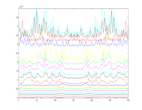
Figure 8: The developing of new modes with the progression towards the free edge

The parameters of the system, $h,E$ and $\mu$, can be combined into one effective stiffness $D=\frac{Eh^{3}}{12(1-\mu^{2})}$ of the plate as the main parameter defining mechanical properties of the system. It has been shown for constant compressing, that increasing stiffness suppresses buckling. Thus as long as $h$ provides the strongest influence on $D$, it seems meaningless to look for buckling in thick stiff membranes. At the same time, thick but soft membranes can be reformulated in terms of thin plates if one rescales the thickness and Young modulus to keep the effective stiffness $D$ the same.

We can provide physical arguments in favor of multi-solution property of spectral equation (33). As long as (33) is derived by the total energy minimization, each mode allowed by (33) realizes a local minimum of the sample’s energy. When the plate is rigid enough, only one single mode exists, and corresponds to the energy minimum that is surely the global one. However, for rather soft plate, we have many energy levels separated by small gaps. It is known that global minimizer of the Föpple-von-Karman elastic energy of a thin plate is not that which is found in real experiments klein1 ; klein2 , where multi-waves solution were encountered instead. Moreover, with decrease of the thickness, the number of waves is increasing and resulting profile is getting more buckled, according to the mentioned experiments. This conclusion is in good agreement with Fig. 5, which can be regarded (since as $D\sim h^{3}$) as cases of two different thicknesses. Apparently, due to fluctuations in the system, the profile of the plate can be understood as the superposition of waves (local minimizers) taken with certain magnitudes accordingly to Boltzmann probabilities.

Let us finalize the paper by some observation which is, to our point of view, beyond just a funny speculation. It is well known that a thin long rod, like a dry noodle, being squeezed at extremities, breaks typically in three parts at two symmetric points to the center ignobel (this work has earned the Ig Nobel prize in 2006). Two maxima of largest amplitudes on the $w(x)$ curve, clearly seen in the Fig. 7 appeared in any of our solutions, in geometric and energetic approaches, in odd or even cases, for many different compressing protocols $q(y)$. It seems naturally to conjecture that points of largest amplitudes in $w(x)$ coincide with the points of maximal stress in the plate. So, we could conjecture that a nonuniformly squeezed plate breaks by proliferation of two basic cracks started at the free surface of points of maximal stress.

Appendix A Minimizing full energy of a plate

In tense state the full energy is determined by the deformation energy and its potential counterpart of distributed forces, $H=U+P$. In the linear approximation the deformation energy of a sample can be written in terms of tension and deformation tensor components (see (21)):

$$U=\frac{1}{2}\int_{V}\bigg{(}\sum_{i}\sigma_{i}\epsilon_{i}+\sum_{i\neq j}\tau_{ij}\gamma_{ij}\bigg{)}dV$$ (37)

where $i=\{x,y,z\},j=\{x,y,z\}$, $i\neq j$, and $\tau_{ij}=\tau_{ji}$, $\gamma_{ij}=\gamma_{ji}$.

Proceeding with Hooke’s law and taking into account the definition of the Young modulus $E$ and the Poisson ratio $\mu$, we get the following explicit expressions:

$$\begin{array}[]{ll}\displaystyle\epsilon_{x}=\frac{\sigma_{x}-\mu\sigma_{y}-\mu\sigma_{z}}{E};&\displaystyle\gamma_{xy}=\frac{2(1+\mu)}{E}\tau_{xy}\vskip 6.0pt plus 2.0pt minus 2.0pt\\ \displaystyle\epsilon_{y}=\frac{\sigma_{y}-\mu\sigma_{x}-\mu\sigma_{z}}{E};&\displaystyle\gamma_{xz}=\frac{2(1+\mu)}{E}\tau_{xz}\vskip 6.0pt plus 2.0pt minus 2.0pt\\ \displaystyle\epsilon_{z}=\frac{\sigma_{z}-\mu\sigma_{x}-\mu\sigma_{y}}{E};&\displaystyle\gamma_{yz}=\frac{2(1+\mu)}{E}\tau_{yz}\end{array}$$ (38)

Then one can reverse (38) and substitute the result into the deformation energy (37). For in-plane compression just until the bifurcation starts, all $z$–components of deformation and stress tensors vanish: $\sigma_{z}$ = $\tau_{x}z$ = $\tau_{y}z$ = 0. It is also worth mentioning that all deformations are considered in a midplane of our thin plate. Thus, we get:

$$U=\frac{E}{2(1-\mu^{2})}\int_{V}\left(\epsilon_{x}^{2}+2\mu\epsilon_{x}\epsilon_{y}+\epsilon_{y}^{2}+\frac{1-\mu}{2}\gamma_{xy}^{2}\right)dV$$ (39)

In linear theory it is possible to treat the components of deformations in terms of linear dependencies of in-plane displacements:

$$\epsilon_{x}=\partial_{x}u,\quad\epsilon_{y}=\partial_{y}v\quad\gamma_{xy}=\partial_{y}u+\partial_{x}v$$

where $u(x,y)$ and $v(x,y)$ are in-plane displacements in $x$ and $y$ directions of the plate correspondingly.

It should be mentioned that we do not take into account deformations due to contraction, as usually is done in pre-buckling state. This effect introduces changes in deformation of second order of $\frac{h}{a}$ and thus could be neglected in the linear approximation. Designate the transverse displacement of midplane points in the instable state as $w(x,y)$ and see how bending (i.e. buckling) induces the local deformations $u_{\rm b}$ and $v_{\bf b}$ at some height $z$ above the midplane. Under the assumption for thin plates that the normal is the same for all the planes of the plate and slightly change the direction, we can write:

$$u=-z\partial_{x}w,\quad v=-z\partial_{y}w$$ (40)

Now it is easy to write down the deformation energy in terms of displacement, $w(x,y)$. Integrating over the thickness of the plate, one arrives at the following expression:

$$U=\frac{D}{2}\int_{-a/2}^{a/2}\int_{-b/2}^{b/2}\Big{\{}\left(\partial^{2}_{xx}w+\partial^{2}_{yy}w\right)^{2}\\ +2(1-\mu)\left(\left(\partial^{2}_{xy}w\right)^{2}-\partial^{2}_{xx}w\partial^{2}_{yy}w\right)\Big{\}}dxdy$$ (41)

where $D=\frac{Eh^{3}}{12(1-\mu^{2})}$ is called a bending stiffness of the plate.

The potential energy of applied forces can be treated as the work needed to get from this state to the reference (unbuckling) state. Let $p(y)$ be the pressure applied at borders of the plate. It can be easily converted to contour force density, $q(y)=hp(y)$, since applied forces are uniform along the plate thickness. The increment of a total work is a sum of a work on $u$ displacement tangential to the plate, and work on $w$ displacement (the force does not perform any work on the displacements normal to the $x$-axis). The tangential part of local force is $dF_{\rm tan}=\frac{p(y)dydz}{\partial_{y}w}$ and the part that performs work on z-displacements is $dF_{z}=p(y)\partial_{x}w\,dydz$. Using the relations (40) one can write the potential energy as the whole work performed:

$$P=\int_{0}^{b}\int_{-h/2}^{h/2}\left(-\frac{z}{\partial_{y}w}+w\right)p(y)\partial_{x}w\,dydz\\ =h\int_{0}^{b}p(y)w\partial_{x}w\,dy,$$ (42)

where we have integrated over the thickness and the work on tangential displacements vanishes due to effectively zero compression energy in the linear approximation. Rewrite (42) as:

$$P=\int\limits_{0}^{b}q(y)\left(w\partial^{2}_{xx}w+\left(\partial_{x}w\right)^{2}\right)dxdy,$$ (43)

Combining (41) and (43) in one energy functional to be minimized, write down the corresponding Euler equation:

$$\frac{D}{2}\Big{\{}\partial^{2}_{xx}\left(2\left(\partial^{2}_{xx}w+\partial^{2}_{yy}w\right)-2(1-\mu)\partial^{2}_{yy}w\right)\\ +\partial^{2}_{yy}\left(2\left(\partial^{2}_{xx}w+\partial^{2}_{yy}w\right)-2(1-\mu)\partial^{2}_{xx}w\right)\\ +2(1-\mu)\partial^{2}_{xy}\left(2\partial^{2}_{xy}w\right)\Big{\}}+3q(y)\partial^{2}_{xx}w=0$$ (44)

and eventually receive a biharmonic equation on $w(x,y)$

$$D\Delta^{2}w+P=0$$ (45)

where $P=3q(y)\partial^{2}_{xx}w$

Appendix B Derivation of boundary conditions

To derive boundary conditions we should first discriminate between two different types of fixation. If the plate is firmly fixed at a border and the rotation over the line of fixing is prohibited, than it is clamp type of fixation and the value $\partial_{\bf n}w$ should vanish, where ${\bf n}$ is a normal towards the border. Otherwise rotation is allowed meaning joint type of fixation. In the last case we demand the absence of any deformations at the edges.

Taking into account the dependencies between bending function $w(x,y)$ and $u-v$ displacements, one can find that the condition of absence of the deformation on $x=-a/2,x=a/2$ edges is equivalent to $\partial^{2}_{xx}w=0$. Similar condition is true for $y=0$ edge.

In linear elasticity regime there are no deformations along the plate in pre-bifurcation states. It means that sizes of a plate in $x$ and $y$ dimensions are kept constant. Thus the 2nd boundary condition says that $z$-displacement nullifies at the boundary, i.e. $w=0$.

While the three edges of a rectangular plate are fixed, the last one, at $y=b$ is kept free to bend. The natural condition here is vanishing of forces and tensions in the direction of growing. Let us write down the Hooke’s law that describes the dependencies between tension and deformation tensors components in the linear regime (compare to (38)):

$$\begin{array}[]{rcl}\displaystyle\sigma_{x}=\displaystyle\frac{E}{1-\mu^{2}}(\epsilon_{x}+\mu\epsilon_{y})&=&\displaystyle\frac{E}{1-\mu^{2}}(\partial_{x}u+\mu\partial_{y}v);\vskip 6.0pt plus 2.0pt minus 2.0pt\\ \displaystyle\sigma_{y}=\displaystyle\frac{E}{1-\mu^{2}}(\mu\epsilon_{x}+\epsilon_{y})&=&\displaystyle\frac{E}{1-\mu^{2}}(\mu\partial_{x}u+\partial_{y}v);\vskip 6.0pt plus 2.0pt minus 2.0pt\\ \displaystyle\tau_{xy}=\displaystyle\frac{E}{2(1+\mu)}\gamma_{xy}&=&\displaystyle\frac{E}{2(1+\mu)}\left(\partial_{y}u+\partial_{x}v\right)\end{array}$$ (46)

According to (46), to vanish tensions towards $y$ axis one should require $\partial_{yy}w+\mu\partial_{xx}w=0$. The same condition for forces can be derived easily, because we take the thickness $h$ of the plate doesn’t change through bending. The change of forces per length unit projection on $y$-axis $df_{y}=\frac{\delta F_{y}}{\delta x}$ acting on the platform with sizes $\delta y,\delta x,h$ near the free edge should be zero:

$$\delta(df_{y})=h(\sigma_{y}(y+dy)-\sigma_{y}(y))+h(\tau_{xy}(y+dy)-\tau_{xy}(y))\\ =h\delta y(\partial_{y}\sigma_{y}+\partial_{y}\tau_{xy})\\ =h\delta y\frac{E}{1-\mu^{2}}\left(\partial_{yyy}w+(2-\mu)\partial_{xxy}w\right)$$ (47)

This gives us the second boundary condition at $y=b$:

$$\partial_{yyy}w+(2-\mu)\partial_{xxy}w=0$$ (48)

Appendix C Numeric approach

To approximate (27) we use symmetric difference quotient with the precision $O(h^{2})$:

$$\frac{u_{i-2}-4u_{i-1}+6u_{i}-4u_{i+1}+u_{i+2}}{h^{4}}\\ -2S_{n}\frac{u_{i-1}-2u_{i}+u_{i+1}}{h^{2}}+S_{n}\left(S_{n}-\frac{q_{i}}{D}\right)u_{i}=0$$ (49)

for $2\leq i\leq N-2$, where $S_{n}=\left(\frac{2\pi n}{a}\right)^{2}$ or $S_{n}=\left(\frac{(2n+1)\pi}{a}\right)^{2}$ and $h=\frac{a}{N}$ is a step size.

The boundary conditions are approximated by right-hand and left-hand quotients (to not to introduce additional points outside the plate). To have precision $O(h^{2})$ they require one more point:

$$\begin{array}[]{l}u_{N}^{\prime}=\displaystyle\frac{3u_{N}+u_{N-2}-4u_{N-1}}{2h}\vskip 6.0pt plus 2.0pt minus 2.0pt\\ u_{0}^{\prime\prime}=\displaystyle\frac{2u_{0}-5u_{1}+4u_{2}-u_{3}}{h^{2}}\vskip 6.0pt plus 2.0pt minus 2.0pt\\ u_{N}^{\prime\prime}=\displaystyle\frac{2u_{N}-5u_{N-1}+4u_{N-2}-u_{N-3}}{h^{2}}\vskip 6.0pt plus 2.0pt minus 2.0pt\\ u_{N}^{\prime\prime\prime}=\displaystyle\frac{5u_{N}-18u_{N-1}+24u_{N-2}-14u_{N-3}+3u_{N-4}}{2h^{3}}\end{array}$$ (50)

We can rewrite (49) using 5-diagonal matrix $A$ having the following form:

$$A=\frac{1}{h^{2}}\left(\begin{matrix}h^{2}&0&0&0&0&0&0&\cdots&0\vskip 6.0pt plus 2.0pt minus 2.0pt\\ 2&-5&4&-1&0&0&0&\cdots&0\vskip 6.0pt plus 2.0pt minus 2.0pt\\ a_{0}^{2}&a_{1}^{2}&a_{2}^{2}&a_{3}^{2}&a_{4}^{2}&0&0&\cdots&0\vskip 6.0pt plus 2.0pt minus 2.0pt\\ 0&a_{1}^{3}&a_{2}^{3}&a_{3}^{3}&a_{4}^{3}&a_{5}^{3}&0&\cdots&0\vskip 6.0pt plus 2.0pt minus 2.0pt\\ 0&0&a_{2}^{4}&a_{3}^{4}&a_{4}^{4}&a_{5}^{4}&a_{6}^{4}&\cdots&0\vskip 6.0pt plus 2.0pt minus 2.0pt\\ &&&\ddots&\ddots&\ddots&\ddots&\ddots\vskip 6.0pt plus 2.0pt minus 2.0pt\\ 0&0&\cdots&0&a_{N-4}^{N-2}&a_{N-3}^{N-2}&a_{N-2}^{N-2}&a_{N-1}^{N-2}&a_{N}^{N-2}\vskip 6.0pt plus 2.0pt minus 2.0pt\\ 0&0&\cdots&0&0&-1&4&-5&2-\mu h^{2}S_{n}\vskip 6.0pt plus 2.0pt minus 2.0pt\\ 0&0&\cdots&0&a_{N-4}^{N}&a_{N-3}^{N}&a_{N-2}^{N}&a_{N-1}^{N}&a_{N}^{N}\end{matrix}\right)$$ (51)

where we have introduced the definitions for $2\leq i\leq N-2$

$$\begin{array}[]{l}a_{i}^{i}=\displaystyle\frac{6}{h^{2}}+4S_{n}+h^{2}S_{n}\left(S_{n}-\frac{q_{i}}{D}\right);\vskip 6.0pt plus 2.0pt minus 2.0pt\\ a_{i-1}^{i}=\displaystyle a_{i+1}^{i}=-2\left(\frac{2}{h^{2}}+S_{n}\right);\vskip 6.0pt plus 2.0pt minus 2.0pt\\ a_{i-2}^{i}=\displaystyle a_{i+2}^{i}=\frac{1}{h^{2}}\end{array}$$ (52)

The explicit form of last row of $A$ is

$$\begin{array}[]{l}a_{N-4}^{N}=\displaystyle\frac{3}{2h};\vskip 6.0pt plus 2.0pt minus 2.0pt\\ a_{N-3}^{N}=\displaystyle\frac{-14}{2h};\vskip 6.0pt plus 2.0pt minus 2.0pt\\ a_{N-2}^{N}=\displaystyle\frac{1}{2h}\left(24-h^{2}S_{n}(2-\mu)\right);\vskip 6.0pt plus 2.0pt minus 2.0pt\\ a_{N-1}^{N}=\displaystyle\frac{1}{2h}\left(-18+4h^{2}S_{n}(2-\mu)\right);\vskip 6.0pt plus 2.0pt minus 2.0pt\\ a_{N}^{N}=\displaystyle\frac{1}{2h}\left(5-3h^{2}S_{n}(2-\mu)\right)\end{array}$$ (53)

References

- (1) S.Nechaev, R.Voituriez, J.Phys. A: Math. Gen. 34 11069-11082 (2001)
- (2) S.Nechaev, O.Vasilyev, J.Phys. A: Math. Gen. 37 3783-3804 (2004)
- (3) V. Borrelli, S. Jabrane, F, Lazarus, and B. Thibert, PNAS, 109 7218 7223 (2012)
- (4) L. S. Levitov, Europhys. Lett. 14, 533 (1991)
- (5) M. Lewicka, L. Mahadevan, M.R. Pakzad, Proceedings of Royal Society A, 467, 402-426 (2011)
- (6) E. Efrati, E. Sharon, R. Kupferman, arXiv:0810.2411
- (7) J. Gemmer, E. Sharon, S. Venkataramani, arXiv:1504.00738
- (8) E. Sharon, B. Roman, M. Marder, G.-S. Shin, and H. L. Swinney, Nature 419, 579 (2002)
- (9) E. Sharon, B. Roman, and H. L. Swinney, Physical Review E 75, 046211 (2007)
- (10) S.K. Nechaev, J. Phys. (A): Math. Gen., 21, 3659-3671 (1988)
- (11) W. Koppenfels, F. Stallman, Praxis der conformen abbildung, (Berlin: Springer, 1959)
- (12) C. Carathéodory, Functiontheorie II, (Basel, 1950)
- (13) V.V.Golubev Lectures on Analytic Theory of Differential Equations (Moscow: GITTL, 1950)
- (14) K. Chandrassekharan, Elliptic Functions (Berlin: Springer, 1985)
- (15) F. Qin, Y. Luo, W. Cai, G.T. Schuster, Geophysics, 57(3), 478-487 (1992)
- (16) R. Nowack, Geophysical Journal International, 110(1), 55-62 (1992)
- (17) H.B. Belgacem, S. Conti, A. DeSimone, S. Müller, Journal of Nonlinear Science, 10(6), 661-685 (2000)
- (18) Y. Klein, S. Venkataramani, E. Sharon, Physical Review Letters, 106(11), 118303 (2011)
- (19) Y. Klein, E. Efrati, E. Sharon, Science, 315(5815), 1116-1120 (2007)
- (20) B. Audoly, S. Neukirch, Physical Review Letters, 95(9), 095505 (2005)