Incremental Query Processing
on Big Data Streams
Abstract
This paper addresses online query processing for large-scale, incremental data analysis on a distributed stream processing engine (DSPE). Our goal is to convert any SQL-like query to an incremental DSPE program automatically. In contrast to other approaches, we derive incremental programs that return accurate results, not approximate answers. This is accomplished by retaining a minimal state during the query evaluation lifetime and by using incremental evaluation techniques to return an accurate snapshot answer at each time interval that depends on the current state and the latest batches of data. Our methods can handle many forms of queries on nested data collections, including iterative and nested queries, group-by with aggregation, and equi-joins. Finally, we report on a prototype implementation of our framework, called MRQL Streaming, running on top of Spark and we experimentally validate the effectiveness of our methods.
Keywords: Incremental Data Processing, Distributed Stream Processing, Big Data, MRQL, Spark.
1 Introduction
In recent years, large volumes of data are being generated, analyzed, and used at an unprecedented scale and rate. Data analysis tools that process these data are typically batch programs that need to work on the complete datasets, thus repeating the computation on existing data when new data are added to the datasets. Consequently, batch processing may be prohibitively expensive for Big Data that change frequently. For example, the Web is evolving at an enormous rate with new Web pages, content, and links added daily. Web graph analysis tools, such as PageRank, which are used extensively by search engines, need to recompute their Web graph measures very frequently since they become outdated very fast. There is a recent interest in incremental Big Data analysis, where data are analyzed in incremental fashion, so that existing results on current data are reused and merged with the results of processing the new data. Incremental data processing can generally achieve better performance and may require less memory than batch processing for many data analysis tasks. It can also be used for analyzing Big Data incrementally, in batches that can fit in memory. Consequently, incremental data processing can also be useful to stream-based applications that need to process continuous streams of data in real-time with low latency, which is not feasible with existing batch analysis tools. For example, the Map-Reduce framework [14], which was designed for batch processing, is ill-suited for certain Big Data workloads, such as real-time analytics, continuous queries, and iterative algorithms. New alternative frameworks have emerged that address the inherent limitations of the Map-Reduce model and perform better for a wider spectrum of workloads. Currently, among them, the most promising frameworks that seem to be good alternatives to Map-Reduce while addressing its drawbacks are Google’s Pregel [29], Apache Spark [40], and Apache Flink [20], which are in-memory distributed computing systems. There are also quite a few emerging distributed stream processing engines (DSPEs) that realize online, low-latency data processing with a series of batch computations at small time intervals, using a continuous streaming system that processes data as they arrive and emits continuous results. To cope with blocking operations and unbounded memory requirements, some of these systems build on the well-established research on data streaming based on sliding windows and incremental operators [4], which includes systems such as Aurora [1] and Telegraph [11], often yielding approximate answers, rather than accurate results. Currently, among these DSPEs, the most popular platforms are Twitter’s (now Apache) Storm [35], Spark’s D-Streams [46], Flink Streaming [20], Apache S4 [42], and Apache Samza [39].
This paper addresses online processing for large-scale, incremental computations on a distributed processing platform. Our goal is to convert any batch data analysis program to an incremental distributed stream processing (DSP) program automatically, without requiring the user to modify this program. We are interested in deriving DSP programs that produce accurate results, rather than approximate answers. To accomplish this task, we would need to carefully analyze the program to identify those parts that can be used to process the incremental batches of data and those parts that can be used to merge the current results with the new results of processing the incremental batches. Such analysis is hard to attain for programs written in an algorithmic programming language but can become more tractable if it is performed on declarative queries. Fortunately, most programmers already prefer to use a higher-level query language, such as Apache Hive [26], to code their distributed data analysis applications, instead of coding them directly in an algorithmic language, such as Java. For instance, Hive is used for over 90% of Facebook Map-Reduce jobs. There are many reasons why programmers prefer query languages. First, it is hard to develop, optimize, and maintain non-trivial applications coded in a general-purpose programming language. Second, given the multitude of the new emerging distributed processing frameworks, such as Spark and Flink, it is hard to tell which one of them will prevail in the near future. Data intensive applications that have been coded in one of these paradigms may have to be rewritten as technologies evolve. Hence, it would be highly desirable to express these applications in a declarative query language that is independent of the underlying distributed platform. Furthermore, the execution of such queries can benefit from cost-based query optimization and automatic parallelism, thus relieving the application developers from the intricacies of Big Data analytics and distributed computing. Therefore, our goal is to convert batch SQL-like queries to incremental DSP programs. We have developed our framework on Apache MRQL [33], because it is both platform-independent and powerful enough to express complex data analysis tasks, such as PageRank, data clustering, and matrix factorization, using SQL-like syntax exclusively. Since we are interested in deriving incremental programs that return accurate results, not approximate answers, our focus is in retaining a minimal state during the query evaluation lifetime and across iterations, and use incremental evaluation techniques to return an accurate snapshot answer at each time interval that depends on the current state and the latest batches of data.
We have developed general, sound methods to transform batch queries to incremental queries. The first step in our approach is to transform a query so that it propagates the join and group-by keys to the query output. This is known as lineage tracking ([5, 6, 13]). That way, the values in the query output are grouped by a key combination, which corresponds the join/group-by keys used in deriving these values during query evaluation. If we also group the new data in the same way, then computations on current data can be combined with the computations on the new data by joining the data on these keys. This approach requires that we can combine computations on data that have the same lineage to derive incremental results. In our framework, this is accomplished by transforming a query to a ’monoid homomorphism’ by extracting the non-homomorphic parts of the query outwards, using algebraic transformation rules, and combine them to form an answer function, which is detached from the rest of the query. We have implemented our incremental processing framework using Apache MRQL [33] on top of Apache Spark Streaming [46], which is an in-memory distributed stream processing platform. Our system is called Incremental MRQL. MRQL is currently the best choice for implementing our framework because other query languages for data-intensive, distributed computations provide limited syntax for operating on data collections, in the form of simple relational joins and group-bys, and cannot express complex data analysis tasks, such as PageRank, data clustering, and matrix factorization, using SQL-like syntax exclusively. Our framework though can be easily adapted to apply to other query languages, such as SQL, XQuery, Jaql, and Hive.
The contribution of this work can be summarized as follows:
-
•
We present a general automated method to convert most distributed data analysis queries to incremental stream processing programs.
-
•
Our methods can handle many forms of queries, including iterative and nested queries, group-by with aggregation, and joins on one-to-many relationships.
-
•
We have extended our framework to handle deletions by using state increments to diminish the state in such a way that the query results would be the same as those we could have gotten on current data after deletion.
-
•
We report on a prototype implementation of our framework using Apache MRQL running on top of Apache Spark Streaming. We show the effectiveness of our method through experiments on four queries: groupBy, join-groupBy, k-means clustering, and PageRank.
The rest of this paper is organized as follows. Section 2 illustrates our approach through examples. Section 3 compares our work with related work. Section 4 describes our earlier work on MRQL query processing. Section 5 defines the algebraic operators used in the MRQL algebra. Section 6 presents transformation rules for converting algebraic terms to a normal form that is easier to analyze. Section 7 describes an inference algorithm that statically infers the merge function that merges the current results with the results of processing the new data. Section 8 describes our method for transforming algebraic terms to propagate all keys used in joins and group-bys to the query output. Section 9 describes an algorithm that pulls the non-homomorphic parts of a query outwards, deriving a homomorphism. Section 10, gives an example of the transformation of a batch query to an incremental query. Section 11 extends our framework to handle data deletion. Section 12 gives some implementation details. Section 13 presents experiments that evaluate the performance of our incremental query processing techniques for four queries.
2 Highlights of our Approach
A dataset in our framework is a bag (multiset) that consists of arbitrarily complex values, which may contain nested bags and hierarchical data, such as XML and JSON fragments. We are considering continuous queries over a number of streaming data sources, , for . A data stream in our framework consists of an initial dataset, followed by a continuous stream of incremental batches that arrive at regular time intervals . In addition to streaming data, there may be other input data sources that remain invariant through time. A streaming query in our framework can be expressed as , where an is a streaming data source. Incremental stream processing is feasible when we can derive the query results at time by simply combining the query results at time (i.e., the current results) with the results of processing the incremental batches only, rather than the entire streams , where is the additive (bag) union. This is possible if can be expressed in terms of (the current query result) and (the incremental query result), that is, when is a homomorphism111We use the term homomorphism throughout the paper as an abbreviation of monoid homomorphism. over . But some queries, such as counting the number of distinct elements in a stream or calculating average values after a group-by, are not homomorphisms. For such queries, we break into two functions and , so that and is a homomorphism. The function is a homomorphism if for some monoid (an associative function with a zero element ). For example, the query that counts the number of distinct elements can be broken into the query that returns the list of distinct elements (a homomorphism), followed by the answer query that counts these elements. Ideally, we would like most of the computation in to be done in , leaving only some computationally inexpensive data mappings to the answer function . Note that, the obvious solution when is equal to and is the union of data sources, is also the worst-case scenario that we try to avoid, since it basically requires to compute the new result from the entire input, . On the other hand, in the special case when is the identity function and is equal to , the output at each time interval can be simply taken to be only , which is the output we would expect to get from a fixed window system (i.e., new batches of output from new batches of input).
If we split into a homomorphism and an answer function , then we can calculate incrementally by storing its results into a state and then using the current state to calculate the next result. Initially, or, if there are initial stream data, . Then, at each time interval , the query answer is calculated from the state, which becomes equal to :
In Spark, for example, the state and the invariant data sources are stored in memory as Distributed DataSets (Spark’s RDDs [45]) and are distributed across the worker nodes. However, the streaming data sources are implemented as Discretized Streams (Spark’s D-Streams [46]), which are also distributed.
Our framework works best for queries whose output is considerably smaller than their input, such as for data analysis queries that aggregate data. Such queries would require a smaller state and impose less processing overhead to .
Figure 1 shows the evaluation of an incremental query over two streaming data sources, where .
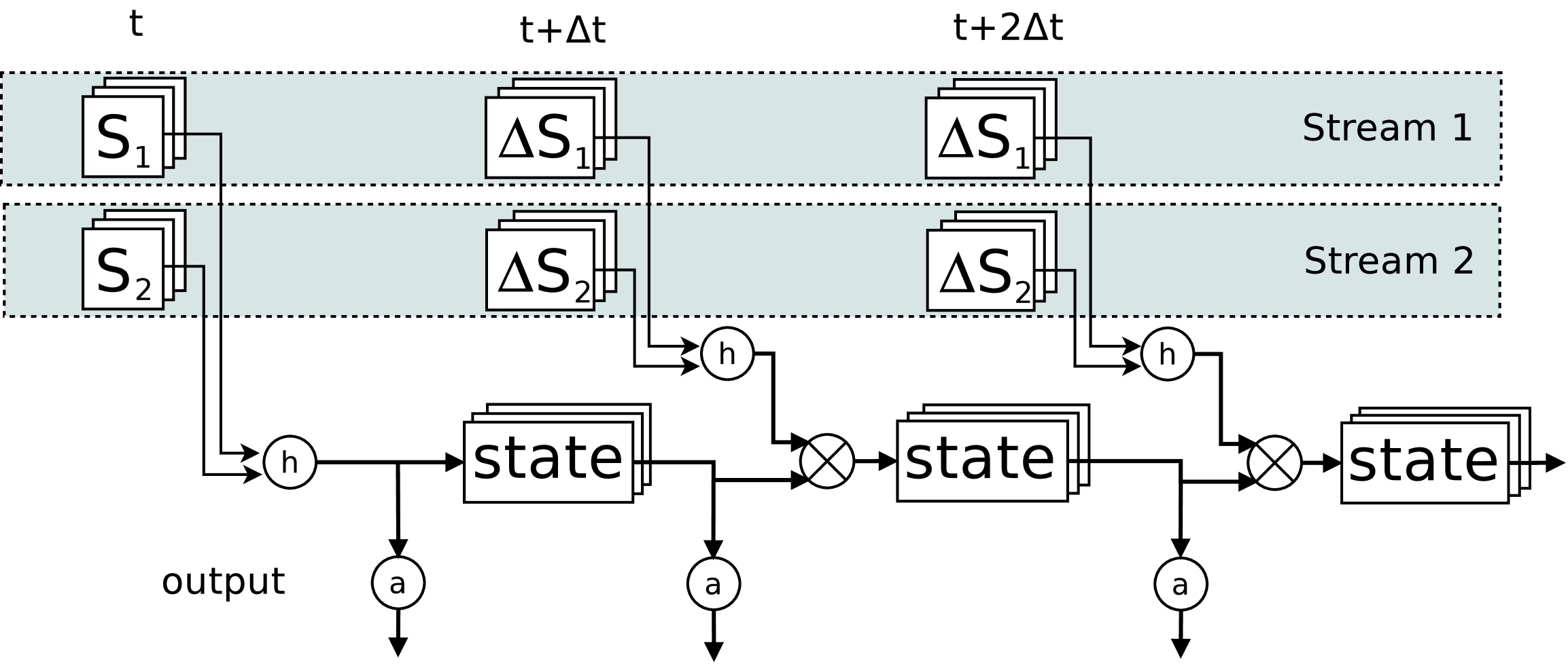
Our query processing system performs the following tasks:
-
1.
It pulls all non-homomorphic parts of a query out from the query, using algebraic transformations.
-
2.
It collects these non-homomorphic parts into an answer function , leaving an algebraic homomorphic term , such that .
-
3.
From the homomorphic algebraic term , our system derives a merge function , such that .
These tasks are, in general, hard to attain for a program expressed in an algorithmic programming language. Instead, these tasks can become more tractable if they are performed on higher-order operations, such as the MRQL query algebra [18, 17]. Although all algebraic operations used in MRQL are homomorphic, their composition may not be. We have developed transformation rules to derive homomorphisms from compositions of homomorphisms, and for pulling non-homomorphic parts outside a query. Our methods can handle most forms of queries on nested data sets, including iterative queries, complex nested queries with any form and any number of nesting levels, general group-bys with aggregations, and general one-to-one and one-to-many equi-joins. Our methods cannot handle non-equi-joins and many-to-many equi-joins, as they are notoriously difficult to implement efficiently in a streaming or an incremental computing environment.
Example
For example, consider the following query (all queries are expressed in MRQL):
where and in are streaming data sources. Unfortunately, is not a homomorphism over and , that is, cannot be expressed in terms of and exclusively. The intrinsic reason behind this is that there is no lineage in the query output that links a pair in the query result to the join key (x.B or y.C) that contributed to this pair. Consequently, there is no way to tell how the new data batches and will contribute to the previous query results if we do not know how these results are related to the inputs and . To compensate, we need to establish links between the query results and the data sources that were used to form their values. This is called lineage tracking and has been used for consistent representation of uncertain data [5] and for propagating annotations in relational queries [6]. In our case, this lineage tracking can be accomplished by propagating all keys used in joins and group-bys along with the values associated with the keys, so that, for each combination of keys, we have one group of result values. For our query, this is done by including the join key x.B as a group-by key. That is, in the following transformed query:
the join key is propagated to the output values so that the avg components, sum and count, are aggregations over groups that correspond to unique combinations of x.A and x.B. It can be shown that this query is a homomorphism over and , provided that the join is not on a many-to-many relationship. In general, a query with joins/group-bys/order-bys will be transformed to a query that injects the join/group-by/order-by keys to the output so that each output value is annotated with a combination of keys. Note that the output of the query is larger than that of the original query because it creates more groups and each group is assigned two values (sum and count), instead of one (avg). This is expected since we extended with lineage tracking. The answer query that gives the final result in is:
that is, it removes the lineage from but also groups the result by the group-by key again and calculates the final avg values. The merge function for the homomorphism is a full outer join on the lineage key that aggregates the matches. It is specified as:
where matches the lineage and is pair and bag projection.
Merging States
The effectiveness of our incremental processing depends on the efficient implementation of the state transformation that merges the previous state with the results of processing the new data, . The merge operation in the previous example can be implemented efficiently as a partitioned join. On Spark, for example, both the state and the new results are kept in the distributed memory of the worker nodes (as RDDs), while the full outer join can be implemented as a coGroup operation, which shuffles the join input data across the worker nodes using hash partitioning. However, when the new state is created by coGroup, it is already partitioned by the join key and is ready to be used for the next call to coGroup to handle the next batch of data. Consequently, only the results of processing the new data, which are typically smaller than the state, would have to be shuffled across the worker nodes before coGroup. Although other queries may require different merge functions, the correlation between the previous state and the results of processing the new data is always based on the lineage keys. Therefore, regardless of the query, we can keep the state partitioned on the lineage keys by simply leaving the new state partitions at the place they were generated. However, the new results would have to be partitioned and shuffled across the working nodes to be combined with the current state.
Our approach is based on the assumption that, since the state is kept in the distributed memory, there will be very little overhead in replacing the current state with a new state, as long as it is not repartitioned. But this assumption may not be valid if the input data or the current state is larger than the available distributed memory. Indeed, one of our goals is to be able to process data larger than the available memory, by processing these data incrementally, in batches that can fit in memory. However, if the state is stored on disk, replacing it with a new state may become prohibitively expensive. Fortunately, there is no need for using a distributed key-value store, such as HBase, to update the state in-place. There is, in fact, a simpler solution: since the state is kept partitioned on the lineage keys, every worker node may store its assigned state partition on its local disk, as a binary file (such as, an HDFS Sequence file) sorted by the lineage key. Then, after the results of processing the new data are distributed to worker nodes (using uniform hashing based on lineage key), each worker node will sort its new data partition by the lineage key and will merge it with its old state (stored on its local disk) to create a new state.
Iteration
Given that many important data analysis and mining algorithms, such as PageRank and k-means clustering, require repetition, we have extended our methods to include repetition, so that these algorithms too can become incremental. A repetition can take the following general form:
where is the fixpoint of the repetition that has initial value . That is, , where applies times. Note that is not necessarily a bag. For example, non-negative Matrix Factorization [22], used in machine learning applications, such as for recommender systems, splits a matrix into two non-negative matrices and . In that case, the fixpoint is the pair , which is refined at every loop step.
An exact incremental solution of the above repetition is only possible if is a homomorphism; a strict requirement that excludes many important iterative algorithms, such as PageRank and k-means clustering. Instead, our approach is to use an approximate solution that works well for iterative queries that improve a solution at each iteration step. As before, we split into a homomorphism , for some monoid , and an answer function , so that and . Let be the current state on input and be the new state on input . An ideal solution would have been to derive the new state incrementally, as , so that the state increment depends on but not on . But this independence from is not always possible for many iterative algorithms. In PageRank, for example, we cannot just calculate the PageRanks of the new data and merge them with the PageRank of the existing data because the new PageRank contributions may have to propagate to the rest of the graph. On the other hand, it would be too expensive to correlate the entire state with at each iteration step. Our compromise is to partially correlate with at each iteration step, and then fully merge with after the iteration. This partial correlation is accomplished with the operation , called diffusion, which is directly derived from the merge function . That is, while returns a new complete state by merging with , the operation returns a new that contains only the part of that is different from . Although is larger than , it is often far smaller than . For instance, if were a bag, would have been a subset of . Based on this analysis, we are using the following approximate algorithm to compute the iteration incrementally:
The diffusion operator must satisfy the property:
that is, when and are merged with , they give the same answer, because discards the parts of that are not joined with , but these parts are embedded back in the answer when we merge with .
For example, PageRank is an iterative algorithm that calculates the PageRank of a graph node as the sum of the incoming PageRank contributions from its neighbors, while its own PageRank is equally distributed to its outgoing neighbors. The PageRank query expressed in MRQL is a simple self-join on the graph, which is optimized into a single group-by operation [18]. For PageRank, the state merging is a full outer join that incorporates the new PageRank contributions to the existing PageRanks. The diffusion operation , on the other hand, propagates the new PageRank contributions from to , that is, from the nodes in to their immediate outgoing neighbors in both and . Thus, at each iteration step, is expanded to , growing one level at a time, in a way similar to breadth-first-search. Consequently, our approximate algorithm propagates PageRanks up to depth , starting from the nodes, and only the affected nodes will be part of the new . The operation is similar to , but with a right-outer join instead of a full outer join. That way, the data from that are not joined with will not appear in the new .
A more complete example is the following query that implements the k-means clustering algorithm by repeatedly deriving new centroids from the old:
where is the input stream of points on the X-Y plane, centroids is the current set of centroids ( cluster centers), and distance is a function that calculates the distance between two points. The initial value of centroids (the … value) can be a bag of random points. The inner select-query in the group-by part assigns the closest centroid to a point s (where [0] returns the first tuple of an ordered list). The outer select-query in the repeat step clusters the data points by their closest centroid, and, for each cluster, a new centroid is calculated from the average values of its points. As in the previous join-groupBy example, the average value of a bag of values is decomposed into a pair that contains the sum and the count of values. That is, the state is a bag of so that the centroids are the bag of points and is the lineage (the group-by key), which is the X-Y coordinates of a centroid. Consequently, the answer query that returns the final result (the centroids) is:
(it does not require a group-by since is the only lineage key), while is:
The merge function is a full outer join, similar to the one used by the join-groupBy example. The diffusion operation though is a right-outer join that discards those state data that do not join with the new data. That is, it is equal to the query without the last union:
But, suppose that one of the group-by or join keys in a query is a floating point number. This is the case with the previous k-means clustering query, because it groups the points by their closest centroids, which contain floating point numbers. The group-by operation itself is not a problem because the centroids are fixed during the group-by. The problem arises when merging the current state with the results of processing the new data. For the k-means query example, the merge function is an equi-join whose join attribute is a centroid, so that the sum and count values associated with the same centroid are brought together from the join inputs and are accumulated. Since the join condition is over attributes with floating point numbers, the join condition will fail in most cases. This problem becomes even worse for the approximate solution, because it uses different sets of centroids and when states are merged. Most iterative queries do not have this problem. The lineage in PageRank, for example, is the node ID, which remains invariant across iterations. For these uncommon queries, such as k-means, that have floating point numbers in their join/group-by/order-by attributes, we use yet another approximation: the join is done based on an “approximate equality” where two floating point numbers are taken to be equal if their difference is below some given threshold. This works well for our approximate solution for iteration because it is based on the assumption that the new solution is approximately equal to the previous one, .
3 Related Work
New frameworks in distributed Big Data analytics have become essential tools to large-scale machine learning and scientific discoveries. Among these frameworks, the Map-Reduce programming model [14] has emerged as a generic, scalable, and cost effective solution for Big Data processing on clusters of commodity hardware. One of the major drawbacks of the Map-Reduce model is that, to simplify reliability and fault tolerance, it does not preserve data in memory between the map and reduce tasks of a Map-Reduce job or across consecutive jobs, which imposes a high overhead to complex workflows and graph algorithms, such as PageRank, which require repetitive Map-Reduce jobs. Recent systems for cloud computing use distributed memory for inter-node communication, such as the main memory Map-Reduce (M3R [38]), Apache Spark [40], Apache Flink [20], Piccolo [36], and distributed GraphLab [28]. Another alternative framework to the Map-Reduce model is the Bulk Synchronous Parallelism (BSP) programming model [44]. The best known implementations of the BSP model for data analysis on the cloud are Google’s Pregel [29], Apache Giraph [21], and Apache Hama [25].
Although the Map-Reduce framework was originally designed for batch processing, there are several recent systems that have extended Map-Reduce with online processing capabilities. Some of these systems build on the well-established research on data streaming based on sliding windows and incremental operators [4], which includes systems such as Aurora [1] and Telegraph [11]. MapReduce Online [12] maintains state in memory for a chain of MapReduce jobs and reacts efficiently to additional input records. It also provides a memoization-aware scheduler to reduce communication across a cluster. Incoop [7] is a Hadoop-based incremental processing system with an incremental storage system that identifies the similarities between the input data of consecutive job runs and splits the input based on the similarity and file content. MapReduce [47] implements incremental iterative Map-Reduce jobs using a store, MRB-Store, that maps input values to the reduce output values. This store is used for detecting delta changes and propagating these changes to the output. Google’s Percolator [35] is a system based on BigTable for incrementally processing updates to a large data set. It updates an index incrementally as new documents are crawled. Microsoft Naiad [32] is a distributed framework for cyclic dataflow programs that facilitates iterative and incremental computations. It is based on differential dataflow computations, which allow incremental computations to have nested iterations. CBP [27] is a continuous bulk processing system on Hadoop that provides a stateful group-wise operator that allows users to easily store and retrieve state during the reduce stage as new data inputs arrive. Their incremental computing PageRank implementation is able to cut running time in half. REX [31] handles iterative computations in which changes in the form of deltas are propagated across iterations and state is updated efficiently. In contrast to our automated approach, REX requires the programmer to explicitly specify how to process deltas, which are handled as first class objects. Trill [10] is a high throughput, low latency streaming query processor for temporal relational data, developed at Microsoft Research. The Reactive Aggregator [43], developed at IBM Research, is a new sliding-window streaming engine that performs many forms of sliding-window aggregation incrementally. In addition to these general data analysis engines, there are many data analysis algorithms that have been implemented incrementally, such as incremental pagerank [15]. Finally, the incremental query processing is related to the problem of incremental view maintenance, which has been extensively studied in the context of relational views (see [23] for a literature survey).
Many novel Big Data stream processing systems, also known as distributed stream processing engines (DSPEs), have emerged recently. The most popular one is Twitter’s Storm [35], which is now part of the Apache ecosystem for Big Data analytics. It provides primitives for transforming streams based on a user-defined topology, consisting of spouts (stream sources) and bolts (which consume input streams and may emit new streams). Other popular DSPE platforms include Spark’s D-Streams [46], Flink Streaming [20], Apache S4 [42], and Apache Samza [39].
In programming languages, self-adjusting computation [2] refers to a technique for compiling batch programs into programs that can automatically respond to changes to their data. It requires the construction of a dependence graph at run-time so that when the computation data changes, the output can be updated by re-evaluating only the affected parts of the computation. In contrast to our work, which requires only the state to reside in memory, self-adjusting computation expects both the input and the output of a computation to reside in memory, which makes it inappropriate for unbounded data in a continuous stream. Furthermore, such dynamic methods impose a run-time storage and computation overhead by maintaining the dependence graph. The main idea in [2] is to manually annotate the parts of the input type that is changeable, and the system will derive an incremental program automatically based on these annotations. Each changeable value is wrapped by a mutator that includes a list of reader closures that need to be evaluated when the value changes. A read operation on a mutator inserts a new closure, while the write operation triggers the evaluation of the closures, which may cause writes to other mutators, etc, resulting to a cascade of closure execution triggered by changed data only. This technique has been extended to handle incremental list insertions (like our work), but it requires the rewriting of all list operations to work on incremental lists. Recently, there is a proof-of-concept implementation of this technique on map-reduce [3], but it was tested on a serial machine. It is doubtful that such dynamic techniques can be efficiently applied to a distributed environment, where a write in one compute node may cause a read in another node. Finally, there is recent work on static incrementalization based on derivatives [8]. In contrast to our work, it assumes that the merge function that combines the previous result with the result on the delta changes uses exactly the same delta changes, a restriction that excludes aggregations and group-bys.
4 Earlier Work: MRQL
Apache MRQL [33] is a query processing and optimization system for large-scale, distributed data analysis. MRQL was originally developed by the author ([18, 17]), but is now an Apache incubating project with many developers and users worldwide. The MRQL language is an SQL-like query language for large-scale data analysis on computer clusters. The MRQL query processing system can evaluate MRQL queries in four modes: in Map-Reduce mode using Apache Hadoop [24], in BSP mode (Bulk Synchronous Parallel model) using Apache Hama [25], in Spark mode using Apache Spark [40], and in Flink mode using Apache Flink [20]. The MRQL query language is powerful enough to express most common data analysis tasks over many forms of raw in-situ data, such as XML and JSON documents, binary files, and CSV documents. The design of MRQL has been influenced by XQuery and ODMG OQL, although it uses SQL-like syntax. In fact, when restricted to XML, MRQL is as powerful as XQuery. MRQL is more powerful than other current high-level Map-Reduce languages, such as Hive [26] and PigLatin [34], since it can operate on more complex data and supports more powerful query constructs, thus eliminating the need for using explicit procedural code. With MRQL, users are able to express complex data analysis tasks, such as PageRank, k-means clustering, matrix factorization, etc, using SQL-like queries exclusively, while the MRQL query processing system is able to compile these queries to efficient Java code that can run on various distributed processing platforms. For example, the PageRank query on raw DBLP XML data, which ranks authors based on the number of citations they have received from other authors, is 16 lines long [17] and can be executed on all the supported platforms as is, without changing the query.
A recent extension to MRQL, called MRQL Streaming, supports the processing of continuous MRQL queries over streams of batch data (that is, data that come in continuous large batches). Before the incremental MRQL work presented in this paper, MRQL Streaming supported traditional window-based streaming based on a fixed window during a specified time interval. Any batch MRQL query can be converted to a window-based streaming query by replacing at least one of the ’source’ calls in the query that access data sources to ‘stream’ calls (with exactly the same call arguments). For example, the query:
groups a stream of points by their coordinate and returns the average values in each group. The MRQL Streaming engine first processes all the existing sequence files in the directory points and then checks this directory periodically for new files. When new files are inserted in the directory, it processes the new batch of data using distributed query processing. MRQL Streaming also supports a stream input format for listening to TCP sockets for text input based on one of the MRQL Parsed Input Formats (XML, JSON, CSV). A query may work on multiple stream sources and multiple batch sources. If there is at least one stream source, the query becomes continuous (it never stops). The output of a continuous query is stored in a file directory, where each file contains the results of processing each batch of streaming data. Currently, MRQL Streaming works on Spark Streaming only but there are current efforts to add support for Storm and Flink Streaming in the near future. The work reported here, called Incremental MRQL, extends the current MRQL Streaming engine with incremental stream processing.
5 The MRQL Algebra
Our compiler translates queries to algebraic terms and then uses rewrite rules to put these algebraic terms into a homomorphic form, which is then used to compute the query results incrementally by combining the previous results with the results of processing the incremental batches.
The MRQL algebra described in this section is a variation of the algebra presented in our previous work [18], but is more suitable for describing our incremental methods. The relational algebra, the nested relational algebra, as well as many other database algebras can be easily translated to our algebra. Our algebra consists of a small number of higher-order homomorphic operators [18], which are defined using structural recursion based on the union representation of bags [19]. Monoid homomorphisms capture the essence of many divide-and-conquer algorithms and can be used as the basis for data parallelism [19].
The first operator, cMap (also known as concat-map or flatten-map in functional programming languages), generalizes the select, project, join, and unnest operators of the nested relational algebra. Given two arbitrary types and , the operation maps a bag of type to a bag of type by applying the function of type to each element of , yielding one bag for each element, and then by merging these bags to form a single bag of type . Using a set former notation on bags, it is expressed as:
| (1) |
or, alternatively, using structural recursion:
Given an arbitrary type that supports value equality (), an arbitrary type , and a bag of type , the operation groups the elements of the bag by their first component and returns a bag of type . For example, groupBy({ (1,“A”), (2,“B”), (1,“C”) }) returns {(1,{“A”,“C”}), (2,{“B”})}. The groupBy operation cannot be defined using a set former notation, but can be defined using structural recursion:
where the parametric monoid is a full outer join that merges groups associated with the same key using the monoid (equal to for groupBy):
where . In other words, the monoid constructs a set of pairs whose unique key is the first pair element. In fact, any bag can be converted to a set using . Note also that is not the same as the nesting , as the latter contains duplicate entries for the key . Unlike nesting, unnesting a groupBy returns the input bag (proven in Appendix A):
| (3) |
Although any join can be expressed as a nested cMap:
this term is not always a homomorphism on both inputs. Instead, MRQL provides a special homomorphic operation for equi-joins and outer joins, , between a bag of type and a bag of type over their first component of a type , which returns a bag of type :
where the product of two monoids, is a monoid that, when applied to two pairs and , returns . That is, the monoid merges two bags of type by unioning together their and values that correspond to the same key . For example, coGroup({ (1,“A”), (2,“B”), (1,“C”) }, { (1,“D”), (2,“E”), (3,“F”) }) returns {(1,({“A”,“C”},{“D”})), (2,({“B”},{“E”})), (3,({ },{“F”}))}. It can be proven (with a proof similar to that of Equation (3)) that both coGroup inputs can be derived from the coGroup result:
and a coGroup is equivalent to a groupBy if one of the inputs is empty:
Aggregations are captured by the operation , which aggregates a bag using a commutative monoid . For example, . This operation is in fact a general homomorphism that can be defined on any monoid with an identity function. We have:
Finally, iteration over the bag of type applies of type to times, yielding a bag of type :
An iteration is a homomorphism as long as is a homomorphism, that is, when .
Definition 1 (MRQL Algebra).
The MRQL algebra consists of terms that take the following form:
where is a monoid on basic types, such as , , , , etc. Function is an anonymous function that may contain such algebraic terms but is not permitted to contain any reference to a stream source, .
The restriction on in Definition 1 excludes non-equi-joins, such as cross products, which require a nested cMap in which the inner cMap is over a data source. This algebra does not include iteration, . Iterations have been discussed in Section 2. In addition, for brevity, this algebra does not include terms for non-streaming input sources, general tuple and record construction and projection, bag union, singleton and empty bag, arithmetic operations, if-then-else expressions, boolean operations, etc.
In addition to these operations, there are a few more algebraic operations that can be expressed as homomorphisms, such as , which is a groupBy followed by a sorting over the group-by key. This operation returns a list, which is represented by the non-commutative monoid list-append, . Mixing multiple collection monoids and operations in the same algebra has been addressed by our previous work [19], and is left out from this paper to keep our analysis simple.
For example, the query used as the first example in Section 2, is translated to the following algebraic term :
where and .
Although all algebraic operators used in MRQL are homomorphisms, their composition may not be. For instance, is not a homomorphism for certain functions , because, in general, cMap does not distribute over . One of our goals is to transform any composition of algebraic operations into a homomorphism.
6 Query Normalization
In an earlier work [18], we have presented general algorithms for unnesting nested queries. For example, consider the following nested query:
A typical method for evaluating this query in a relational system is to first group Y by y.B, yielding pairs of y.B and sum(y.C), and then to join the result with X on x.A=y.B using a left-outer join, removing all those matches whose x.D is below the sum. But, in our framework, this query is translated into:
| cMap( | (k,(xs,ys)). cMap( | x. | if x.D reduce(+,ys) |
| then {x} | |||
| else { }, xs), | |||
| coGroup( | cMap( x. {(x.A,x)}, X ), | ||
| cMap( y. {(y.B,y.C)}, Y ) ) ) |
That is, the query unnesting is done with a left-outer join, which is captured concisely by the coGroup operation without the need for using an additional group-by operation or handling null values. This unnesting technique was generalized to handle arbitrary nested queries, at any place, number, and nesting level (the reader is referred to our earlier work [18] for details).
The algebraic terms derived from MRQL queries can be normalized using the following rule:
| (4) |
which fuses two cascaded cMaps into a nested cMap, thus avoiding the construction of the intermediate bag. This rule can be proven directly from the cMap definition in Equation (1):
If we apply the transformation (4) repeatedly, and given that we can always use the identity in places where there is no cMap between groupBy/coGroup operations, any algebraic terms in Definition 1 can be normalized into the following form:
Definition 2 (Normalized MRQL Algebra).
The normalized MRQL algebra consists of terms that take the following form:
where function is an anonymous function that does not contain any reference to a stream source, .
The query body is a tree of groupBy/coGroup operations connected via cMaps.
| (5a) (5b) (5c) (5d) (5e) (5f) (5g) (5h) |
7 Monoid Inference
One of our tasks is, given an algebraic term , where an is a streaming data source, to prove that is a homomorphism by deriving a monoid such that:
| (6) |
We have developed a monoid inference system, inspired by type inference systems used in programming languages. We use the judgment to indicate that is a monoid homomorphism with a merge function under the environment , which binds variables to monoids. The notation extracts the binding of the variable , while extends the environment with a new binding from to . Equation (6) can now be expressed as the judgment:
If a term is invariant under change, such as an invariant data source, it is associated with the special monoid :
Our monoid inference algorithm is a heuristic algorithm that annotates terms with monoids (when possible). It is very similar to type inference. Most of our inference rules are expressed as fractions: the denominator (below the line) contains the premises (separated by comma) and the numerator (above the line) is the conclusion. For example, the rule indicates that . Figure 2 gives some of the inference rules. More rules will be given in Lemma 1. Rules (5c) through (5f) are derived directly from the algebraic definition of the operators. Rule (5a) retrieves the associated monoid of a variable from the environment . Rule (5b) indicates that if all the variables in a term are invariant, then so is . Rule (5h) indicates that a cMap over a groupBy is a homomorphism as long as its functional argument is a homomorphism. It can be proven as follows:
8 Injecting Lineage Tracking
There are two tasks that need to be accomplished to achieve our goal of transforming an algebraic term into a homomorphism: 1) transform the algebraic term in such a way that it propagates all keys used in joins and group-bys to the query output, and 2) pull the non-homomorphic parts out of the algebraic term so that it becomes a homomorphism. In this section, we address the first task.
We will transform the algebraic terms given in Definition 2 in such a way that they propagate the join and the group-by keys. That is, each value returned by these terms is annotated with a lineage , as a pair , where takes the following form:
That is, the lineage of the query result is the tree of the groupBy and coGroup keys that are used in deriving the result (one key for each groupBy and coGroup operation). The lineage tree has the same shape as the groupBy/coGroup tree of the query. We transform a query in such a way that, if the output of the query is for some type , then the transformed query will have output . Furthermore, if the the output is a non-collection type , then the transformed query will also have output , which separates the contributions to associated with each combination of group-by/join keys.
Algorithm 1 (Lineage Annotation).
Input: a normalized query term defined in Definition 2
Output: a term annotated with a lineage
(7a)
(7b)
(7c)
(7d)
(7e)
(7f)
(7g)
(7h)
where sMap1, sMap2, sMap3, swap, and mix are defined as follows:
| (8a) | ||||
| (8b) | ||||
| (8c) | ||||
| (8d) | ||||
| (8e) | ||||
A query in our framework is transformed in such a way that it propagates the lineage from the data stream sources to the query output, starting with the empty lineage at the sources and extended with the join and group-by keys. The sMap1 operation is a cMap that propagates the input lineage to the output as is. The sMap2 operation is a cMap that extends the input lineage with a groupBy/coGroup key . The lineage propagation is done by the cMap Rules (7c) and (7h). Rule (7c) applies to the outer query cMap that produces the query output. It simply propagates the lineage from the cMap input to the output. Rule (7h) applies to a cMap that returns the input of a groupBy or coGroup. The output of this cMap must be a bag of key-value pairs, as is expected by a groupBy or a coGroup. Thus, Rule (7h) extends the lineage with a new key and prepares the cMap output for the enclosing groupBy or coGroup. This is done by translating cMap to sMap2. Rule (7b) indicates that a total aggregation becomes a group-by aggregation by aggregating the values of each group associated with a different lineage . Rule (7e) translates a groupBy on a key to a groupBy on the entire lineage (which includes the groupBy key). Rule (7f) translates a coGroup on a key to a coGroup on the entire lineage, but it is done using the function mix (defined in (8e) because the left input lineage is not necessarily compatible with the right input lineage . Given this, Rule (7f) generates a coGroup on the join key first, and then, for each join key , it groups the left and right join matches by and respectively, so that the output contains unique lineage key combinations, . Finally, Rule (7g) annotates each value of the input stream with the empty lineage .
We will prove next that the transformed query is a homomorphism. We first prove that the generated sMap1 and sMap2 in are homomorphisms, provided that their functional arguments are homomorphisms. More specifically, we prove the following judgments:
Lemma 1 (Transformed Term Judgments).
| (9a) | |||
| (9b) | |||
| (9c) | |||
| (9d) | |||
| (9e) | |||
The proof of this Lemma is given in Appendix A.
Definition 3 (Query Merger Monoid).
The query merger monoid of a normalized query term is defined as follows:
where the monoid in the last equation comes from in Equation (9a).
Based on Lemma 1, we can now prove that the transformed query is a homomorphism:
Theorem 1 (Homomorphism).
The proof is given in Appendix A.
Definition 4 (Query Answer).
The following theorem proves that returns the same answer as :
Theorem 2 (Correctness).
The over the state returns the same result as the original query , where is defined in Definition 2:
| for | (11) |
The proof of this theorem is given in Appendix A.
8.1 Restricting Joins
Theorem 1 indicates that a query transformed by Algorithm 1 is a homomorphism if the cMap functional arguments in the query satisfy the premises in Judgment (9a) and (9b). But, consider the following join:
Our monoid inference system can not prove that the functional argument of this cMap is a homomorphism on both and . This is expected because this join could be a many-to-many join, which we know can not be a homomorphism. Since we have given up on handling many-to-many joins, we want to extend the monoid inference algorithm to always assume that every join is a one-to-one or one-to-many join and draw inferences based on this assumption.
We have already seen in Section 7 that if a term is invariant under change, such as an invariant data source, it is associated with the special monoid . We can also use the annotation to denote certain functional dependencies, such as on a bag of type , which indicates that the second component of a pair in depends on the first. This dependency is captured by annotating with the monoid , which indicates that each group remains invariant under change, implying that the group-by key is also a unique key of . That is, if and , then in Definition (5) must have so that , otherwise it will be an error. This means that we can not have two different groups associated with the same key . Given that a groupBy over a singleton gives a singleton group, each group returned from a groupBy is a singleton that remains invariant. A similar functional dependency can also apply to a join between of type and of type , which is a of type . To indicate that this join is one-to-one or one-to-many, we annotate with the monoid , which enforces the constraint that the bag in be either empty or singleton, that is, at most one element can be joined with over a key . This is because the and values that are joined over the same key are merged with and , respectively, as indicated by . Therefore, to incorporate the assumption that all joins are one-to-one or one-to-many in the monoid inference system, we have to replace Judgment (5g) with the following judgment:
| (12) |
Given this judgment, the cMap input of our join example will be annotated with , which means that and will be annotated with and , respectively (ie, is invariant). Based on these annotations, the functional argument satisfies the premise in Judgment (9b) since it is annotated with .
8.2 Handling Iterative Queries
The approximate algorithm that processes iterations incrementally, presented in Section 2, requires an additional operation, called the diffusion operator , that satisfies the property:
Our goal is to define in terms of in such a way that contains only those parts of that changed from .
Definition 5 (Diffusion).
The diffusion of a monoid is defined as follows:
where is a right-outer join defined as follows:
This satisfies the desired property, (proven in Appendix A).
9 Non-Homomorphic Terms
Theorem 2 indicates that the terms generated by the transformations (7a) through (7h) are homomorphisms as long as the premises of the judgements in Lemma 1 are true. These premises indicate that the cMap functional arguments must be homomorphisms too. We want the operations that cannot be annotated with a monoid to be transformed so that the non-homomorphic parts of the operation are pulled outwards from the query using rewrite rules. We achieve this with the help of kMap:
which is a cMap that propagates the lineage as is. In our framework, all non-homomorphic parts take the form of a kMap and are accumulated into one kMap using
More specifically, we first split each non-homomorphic cMap to a composition of a kMap and a cMap so that the latter cMap is a homomorphism, and then we pull and merge kMaps. Consider the term , which creates a new lineage from the old . In our framework, we find the largest subterms in the algebraic term , namely , that are homomorphisms. This is accomplished by traversing the tree that represents the term , starting from the root, and by checking if the node can be inferred to be a homomorphism. If it is, the node is replaced with a new variable. Thus, is mapped to a term , for some term , and the terms are replaced with variables when is pulled outwards:
The kMaps are combined and are pulled outwards from the query using the following rewrite rules:
where . Rewrite rules as these, when applied repeatedly, can pull out and combine the non-homomorphic parts of a query, leaving a homomorphism whose merge function can be derived from our annotation rules.
10 An Example
Consider again the algebraic term , presented at the end of Section 5. If we apply the transformations in Equations (7a) through (7h), we derive the following term term , which propagates the join and group-by keys to the query output:
| (13) | |||
where and . If we expand sMap1, sMap2, swap, and mix, then the transformed query is:
where is
The output lineage is , where and are groupBy and coGroup keys. But, and since the key is . Consequently, the transformed query becomes:
We now check if the transformed query (13) is a homomorphism. Both coGroup inputs in (13) are sMap2 terms, annotated with , which means that, based on Equation (5g), the coGroup is annotated with . From Equation (9b), the sMap2 operation is annotated with as long as is annotated with . Hence, the groupBy operation is annotated with , based on Equation (5f). Unfortunately, based on Equation (8a), the sMap1 term is not a homomorphism as is, because is not a homomorphism over . Based on the methods described in Section 9 that factor out non-homomorhic parts from terms, the sMap1 term is broken into two terms , where is:
This is equivalent to the homomorphism given in Section 2.
In addition, from Definition 4, the answer function is . Therefore, the answer function , combined with the non-homomorphic part of the query is:
This is equivalent to the answer query given in Section 2. Finally, is a homomorphism annotated with , because the reduce terms are annotated with (from Equation (5c)) and we have a pair of homomorphisms. This is equivalent to the merge function given in Section 2, implemented as a partitioned join combined with aggregation.
11 Handling Deletions
Our framework can be easily extended to handle deletion of existing data from an input stream, in addition to insertion of new data. To handle both insertions and deletions, a data stream in our framework consists of an initial data set, followed by a continuous stream of incremental batches and a continuous stream of decremental batches that arrive at regular time intervals . Then, the stream data at time is , where is bag difference, which satisfies . (An element appears in as many times as it appears in , minus the number of times it appears in .) This dual stream of updates, can be implemented as a single stream that contains updates tagged with + or -, to indicate insertion or deletion. Alternatively, a stream data source may monitor two separate directories, one for insertions and another for deletions, so that if a new file is created, it will be treated as a new batch of insertions or deletions, depending on the directory. In our framework, we require that , that is, we can only delete values that have already appeared in the stream in larger or equal multiplicities. This restriction implies that there is a bag such that . Without this restriction, it would be hard to diminish the query results on by the results on to calculate the new results.
Definition 6 (Diminisher).
The diminisher of a monoid is defined as follows:
where is a left-outer join defined as follows:
Note that a diminisher is not a monoid.
Theorem 3.
For all .
The proof is given in Appendix A. For , it implies that .
Theorem 4.
If and for all
,
then .
Proof.
Since , then there must be such that . Thus, . Then,
This theorem indicates that, to process the deletions , we can simply use the same methods as for insertions, but using the diminishing function for merging the state, instead of . That is, we can use the same functions and , but now the state is diminished as follows:
For example, the join-groupby query used in Section 2 must now use the merging, , equal to:
12 Implementation
We have implemented our incremental processing framework using Apache MRQL [33] on top of Apache Spark Streaming [46]. The Spark streaming engine monitors the file directories used as stream sources in an MRQL query, and when a new file is inserted in one of these directories or the modification time of a file changes, it triggers the MRQL query processor to process the new files, based on the state derived from the previous step, and creates a new state.
We have introduced a new physical operator, called Incr, which is a stateful operator that updates a state. More specifically, every instance of this operation is annotated with a state number and is associated with a state, , of type . The operation , where is a state transition function of type and is the initial state of type , has the following semantics:
with , initially. Note that the states are preserved across the Inc calls and are modified by these calls.
Recall that, in our framework, we break a query into a homomorphism and an answer function , and we evaluate the query incrementally using:
at every time interval, where, initially, . This is implemented using the following physical plan:
For an iteration , we use the approximate solution, described in Section 2: we split into a homomorphism , for some monoid , and a function , and we derive a diffusion operator :
13 Performance Evaluation
The system described in this paper is available as part of the latest official MRQL release (MRQL 0.9.6). We have experimentally validated the effectiveness of our methods using four queries: groupBy, join-groupBy, k-means clustering, and PageRank. The platform used for our evaluations is a small cluster of 9 Linux servers, connected through a Gigabit Ethernet switch. Each server has 4 Xeon cores at 3.2GHz with 4GB memory. For our experiments, we used Hadoop 2.2.0 (Yarn) and Spark 1.6.0. The cluster frontend was used exclusively as a NameNode/ResourceManager, while the rest 8 compute nodes were used as DataNodes/NodeManagers. For our experiments, we used all the available 32 cores of the compute nodes for Spark tasks.
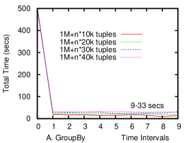
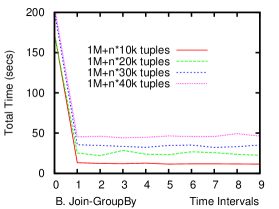
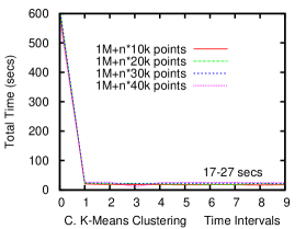
The data streams used by the first 3 queries (groupBy, join-groupBy, and k-means clustering) consist of a large set of initial data, which is used to initialize the state, followed by a sequence of 9 equal-size batches of data (the increments). The experiments were repeated for increments of size 10K, 20K, 30K, and 40K tuples, always starting with a fresh state (constructed from the initial data only). The performance results are shown in Figure 3. The -axis represents the time points when we get new batches of data in the stream. At time , we have the processing of the initial data and the construction of the initial state. Then, the 9 increments arrive at the time points through . The -axis is the query execution time, and there are 4 plots, one for each increment size.
The join-groupBy and the k-means clustering queries are given in Section 2. The groupBy query is ‘select (x,avg(y)) from (x,y) in group by x’. The datasets used for both the groupBy and join-groupBy queries consist of pairs of random integers between 0 and 10000. The groupBy initial dataset has size 1M tuples, while the two join-groupBy inputs have size 100K tuples. The datasets used for the k-means query consist of random points in 4 squares that have in or and in or . Thus, the 4 centroids are expected to be , , , and . This also means that the state contains 4 centroids only. The initial dataset for k-means contains 1M points and the k-means query uses 10 iteration steps. The k-means incremental program uses the approximate solution described in Section 2 based on approximate floating point equality.
From Figure 3, we can see that processing incremental batches of data can give an order of magnitude speed-up compared to processing all the data each time. Furthermore, the time to process each increment does not substantially increase through time, despite that the state grows with new data each time (in the case of the groupBy and join-groupBy queries). This happens because merging states is done with a partitioned join (implemented as a coGroup in Spark) so that the new state created by coGroup is already partitioned by the join key and is ready to be used for the next coGroup to handle the next increment. Consequently, only the results of processing the new data, which are typically smaller than the state, are shuffled across the worker nodes before coGroup. This makes the incremental processing time largely independent of the state size in most cases since data shuffling is the most prevalent factor in main-memory distributed processing systems.
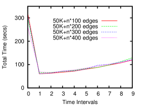
We have also evaluated our system on a PageRank query on random graphs generated by the R-MAT algorithm [9] using the Kronecker graph generator parameters: a=0.30, b=0.25, c=0.25, and d=0.20. The PageRank query expressed in MRQL is a simple self-join on the graph, which is optimized into a single group-by operation. (The MRQL PageRank query is given in [18].) The PageRanks were calculated in 10 iteration steps. This time, the initial graph used in our evaluations had size 5K nodes with 50K edges and the four different increments had sizes 100 nodes with 100, 200, 300, and 400 edges, respectively. The performance results are shown in Figure 4. We believe that the reason that we did not get a flat line for our incremental PageRank implementation was due to the lack of sufficient memory tuning. In Spark, cached RDDs and D-Streams are not automatically garbage-collected; instead, Spark leaves it to the programmer to cache the queued operations in memory if their results are used multiple times, and to dispose the cache later. This is reminiscent to legacy programming languages, such as C, that did not support GC. Removing all memory leaks is very crucial to continuous stream processing, and, if not done properly, it will eventually cause the system to run out of memory. We are planning to fine-tune our streaming engine to remove all these memory leaks.
14 Conclusion and Future Work
We have presented a general framework for translating batch MRQL queries to incremental DSPE programs. In contrast to other systems, our methods are completely automated and are formally proven to be correct. In addition to incremental query processing on a DSPE platform, our framework can also be used on a batch distributed system to process data larger than the available distributed memory, by processing these data incrementally, in batches that can fit in memory. Although our methods are described using the unconventional MRQL algebra, instead of the nested relational algebra, we believe that many other similar query systems can use our framework by simply translating their algebraic operators to the MRQL operators, then, using our framework as is, and, finally, translating the resulting operations back to their own algebra.
As a future work, we are planning to use an in-memory key-value store to
update the state in place, instead of replacing the entire state with
a new one every time we process a new batch of data. Spark
Streaming, in fact, already supports an operation updateStateByKey
operation, which allows to maintain an arbitrary state while
continuously updating it with new data. We believe that this will
considerably improve the performance of queries that require large
states, such as PageRank. Finally, in the near future, we are planning to add support
for more DSPE platforms in Incremental MRQL, such as Storm and Flink Streaming.
Acknowledgments:
This work is supported in part by the National Science Foundation
under the grant CCF-1117369.
Some of our performance evaluations were performed at the Chameleon cloud
computing infrastructure, supported by NSF, https://www.chameleoncloud.org/.
References
- [1] D. J. Abadi, D. Carney, U. Cetintemel, et al. Aurora: A New Model and Architecture for Data Stream Management. In VLDB Journal, 12(2):120–139, 2003.
- [2] U. A. Acar, G. E. Blelloch, M. Blume, R. Harper, and K. Tangwongsan. An Experimental Analysis of Self-Adjusting Computation. In ACM Trans. Prog. Lang. Sys., 32(1):3:1–53, 2009.
- [3] U. A. Acar and Y. Chen. Streaming Big Data with Self-Adjusting Computation. In Workshop on Data Driven Functional Programming (DDFP), 2013.
- [4] B. Babcock, S. Babu, M. Datar, R. Motwani, and J. Widom. Models and Issues in Data Stream Systems. In Symposium on Principles of Database Systems (PODS), pages 1–16, 2002.
- [5] O. Benjelloun, A. D. Sarma, A. Halevy, and J. Widom. ULDBs: Databases with Uncertainty and Lineage. In International Conference on Very Large Data Bases (VLDB), pages 953–964, 2006.
- [6] D. Bhagwat, L. Chiticariu, W. C. Tan, and G. Vijayvargiya. An Annotation Management System for Relational Databases. In International Conference on Very Large Data Bases (VLDB), pages 900–911, 2004.
- [7] P. Bhatotia, A. Wieder, R. Rodrigues, U. A. Acar, and R. Pasquin. Incoop: Mapreduce for Incremental Computations. In ACM Symposium on Cloud Computing (SoCC), 2011.
- [8] Y. Cai, P. G. Giarrusso, T. Rendel, and K. Ostermann. A Theory of Changes for Higher-Order Languages. Incrementalizing -Calculi by Static Differentiation. In ACM SIGPLAN Conference on Programming Language Design and Implementation (PLDI), pages 145-155, 2014.
- [9] D. Chakrabarti, Y. Zhan, and C. Faloutsos. R-MAT: A Recursive Model for Graph Mining. In Fourth SIAM International Conference on Data Mining (SDM), pages 442–446, 2004.
- [10] B. Chandramouli, J. Goldstein, M. Barnett, R. DeLine, D. Fisher, J. C. Platt, J. F. Terwilliger, J. Wernsing. Trill: A High-Performance Incremental Query Processor for Diverse Analytics. In International Conference on Very Large Data Bases (VLDB), pages 401–412, 2014.
- [11] S. Chandrasekaran, O. Cooper, A. Deshpande, M. J. Franklin, J. M. Hellerstein, W. Hong, S. Krishnamurthy, S. Madden, V. Raman, F. Reiss, and M. Shah. TelegraphCQ: Continuous Data flow Processing for an Uncertain World. In Conference on Innovative Data System Research (CIDR), 2003.
- [12] T. Condie, N. Conway, P. Alvaro, J. M. Hellerstein, K. Elmeleegy, and R. Sears. Mapreduce Online. In USENIX Symposium on Networked Systems Design and Implementation (NSDI), 10(4), 2010.
- [13] Y. Cui and J. Widom. Lineage Tracing for General Data Warehouse Transformations. In International Conference on Very Large Data Bases (VLDB), pages 471–480, 2001.
- [14] J. Dean and S. Ghemawat. MapReduce: Simplified Data Processing on Large Clusters. In Symposium on Operating System Design and Implementation (OSDI), 2004.
- [15] P. Desikan, N. Pathak, J. Srivastava, and V. Kumar Incremental PageRank Computation on Evolving Graphs. In International conference on World Wide Web (WWW), pages 1094–1095, 2005.
- [16] L. Fegaras. Supporting Bulk Synchronous Parallelism in Map-Reduce Queries. In International Workshop on Data Intensive Computing in the Clouds (DataCloud), 2012.
- [17] L. Fegaras, C. Li, U. Gupta, and J. J. Philip. XML Query Optimization in Map-Reduce. In International Workshop on the Web and Databases (WebDB), 2011.
- [18] L. Fegaras, C. Li, and U. Gupta. An Optimization Framework for Map-Reduce Queries. In International Conference on Extending Database Technology (EDBT), pages 26–37, 2012.
- [19] L. Fegaras and D. Maier. Optimizing Object Queries Using an Effective Calculus. In ACM Transactions on Database Systems (TODS), 25(4):457–516, 2000.
- [20] Apache Flink. http://flink.apache.org/.
- [21] Apache Giraph. http://giraph.apache.org/.
- [22] A. Ghoting, R. Krishnamurthy, E. Pednault, B. Reinwald, V. Sindhwani, S. Tatikonda, Y. Tian, and S. Vaithyanathan. SystemML: Declarative Machine Learning on MapReduce. In IEEE International Conference on Data Engineering (ICDE), pages 231–242, 2011.
- [23] A. Gupta and I. S. Mumick. Maintenance of Materialized Views: Problems, Techniques, and Applications. In IEEE Bulletin on Data Engineering, 18(2):145–157, 1995.
- [24] Apache Hadoop. http://hadoop.apache.org/.
- [25] Apache Hama. http://hama.apache.org/.
- [26] Apache Hive. http://hive.apache.org/.
- [27] D. Logothetis, C. Olston, B. Reed, K.C. Webb, and K. Yocum. Stateful Bulk Processing for Incremental Analytics. In ACM Symposium on Cloud Computing (SoCC), 2010.
- [28] Y. Low, J. Gonzalez, A. Kyrola, D. Bickson, C. Guestrin, and J. M. Hellerstein. Distributed GraphLab: A Framework for Machine Learning and Data Mining in the Cloud. In Proceedings of the VLDB Endowment, 5(8):716-727, 2012.
- [29] G. Malewicz, M. H. Austern, A. J.C Bik, J. C. Dehnert, I. Horn, N. Leiser, and G. Czajkowski. Pregel: a System for Large-Scale Graph Processing. In ACM symposium on Principles of Distributed Computing (PODC), 2009.
- [30] F. McSherry, D. G. Murray, R. Isaacs, and M. Isard. Differential Dataflow. In Conference on Innovative Data System Research (CIDR), 2013.
- [31] S. R. Mihaylov, Z. G. Ives, and S. Guha. REX: Recursive, Delta-Based Data-Centric Computation. In Proceedings of the VLDB Endowment, 5(11):1280-1291, 2012.
- [32] D. G. Murray, F. McSherry, R. Isaacs, M. Isard, P. Barham, and M. Abadi. Naiad: a Timely Dataflow System. In ACM Symposium on Operating Systems Principles (SOSP), 2013.
- [33] Apache MRQL (incubating). http://mrql.incubator.apache.org/.
- [34] C. Olston, B. Reed, U. Srivastava, R. Kumar, and A. Tomkins. Pig Latin: a not-so-Foreign Language for Data Processing. In ACM SIGMOD International Conference on Management of Data, pages 1099-1110, 2008.
- [35] D. Peng and F. Dabek. Large-scale Incremental Processing using Distributed Transactions and Notifications. In Symposium on Operating System Design and Implementation (OSDI), 2010.
- [36] R. Power and J. Li. Piccolo: Building Fast, Distributed Programs with Partitioned Tables. In Symposium on Operating System Design and Implementation (OSDI), 2010.
- [37] Ramalingam, G. and Reps, T. A Categorized Bibliography on Incremental Computation. In Principles of Programming Languages (POPL), 1993, pp. 502–510.
- [38] A. Shinnar, D. Cunningham, B. Herta, and V. Saraswat. M3R: Increased Performance for In-Memory Hadoop Jobs. In Proceedings of the VLDB Endowment, 5(12):1736-1747, 2012.
- [39] Apache Samza. http://samza.apache.org/
- [40] Apache Spark. http://spark.apache.org/.
- [41] Apache Storm: A System for Processing Streaming Data in Real Time. http://hortonworks.com/hadoop/storm/.
- [42] Apache S4 (incubating): A Distributed Stream Computing Platform. http://incubator.apache.org/s4/.
- [43] K. Tangwongsan, M. Hirzel, S. Schneider, and K.-L. Wu. General Incremental Sliding-Window Aggregation. In Proceedings of the VLDB Endowment, 8(7):702-713, 2015.
- [44] L. G. Valiant. A Bridging Model for Parallel Computation. In Communications of the ACM (CACM), 33(8):103-111, August 1990.
- [45] M. Zaharia, M. Chowdhury, T. Das, A. Dave, J. Ma, M. McCauley, M. J. Franklin, S. Shenker, and I. Stoica. Resilient Distributed Datasets: A Fault-Tolerant Abstraction for In-Memory Cluster Computing. In USENIX Symposium on Networked Systems Design and Implementation (NSDI), 2012.
- [46] M. Zaharia, T. Das, H. Li, T. Hunter, S. Shenker, and I. Stoica. Discretized Streams: Fault-Tolerant Streaming Computation at Scale. In Symposium on Operating Systems Principles (SOSP), 2013.
- [47] Y. Zhang, S. Chen, Q. Wang, and G. Yu. i2 MapReduce: Incremental MapReduce for Mining Evolving Big Data. In IEEE Transactions on Knowledge and Data Engineering (TKDE), 27(7):1906-1919, 2015.
Appendix A Proofs
Proof of Equation (3).
We will use structural induction. The inductive step
can be proven as follows. Let and . Then, for
| (14) | ||||
we have, , because for each group-by key , there is at most one and at most one . Then, we have:
Proof of Lemma 1 (Transformed Term Judgments).
Theorem 1 (Homomorphism).
Proof.
We will prove Theorem 2 using the following lemma:
Lemma 2.
Proof.
Theorem 2 (Correctness).
Proof.
To prove Equation (11), we first prove from Equations (7g) and (7h). If , then
If , then using Equations (7h), (7e), (15a) and (15c):
If , then using Equations (7h), (7f), (15b) and (15d)):
We now prove Equation (11) using induction on . Based on Definition 4, we have three cases. When , then for :
| (from induction hypothesis) | |||
For , we have:
For , we have:
where
It is easy to prove by induction that for we have . Then,
The proof for is similar. For , and for or (the proof is easier for ), we have:
from the previous proofs for and. ∎
Theorem 3.
For all .
Proof.
We will prove this for only: