Orbital Spectrum Analysis of Non-Axisymmetric Perturbations of the Guiding-Center Particle Motion in Axisymmetric Equilibria

Abstract

The presence of non-axisymmetric perturbations in an axisymmetric magnetic field equilibrium renders the Guiding Center (GC) particle motion non-integrable and may result in particle, energy and momentum redistribution, due to resonance mechanisms. We analyse these perturbations in terms of their spectrum, as observed by the particles in the frame of unperturbed GC motion. We calculate semi-analytically the exact locations and strength of resonant spectral components of multiple perturbations. The presented Orbital Spectrum Analysis (OSA) method is based on an exact Action-Angle transform that fully takes into account Finite Orbit Width (FOW) effects. The method provides insight into the particle dynamics and enables the prediction of the effect of any perturbation to all different types of particles and orbits in a given, analytically or numerically calculated, axisymmetric equilibrium.

I Introduction

Guiding Center (GC) theory has been widely used for more than four decades as the basis for the study of single and collective particle dynamics in toroidal magnetic fields utilized in fusion devices Ref. 1]. The theory has been originally formulated in a non-canocical Ref. 2] description which was later extended to a canonical one Ref. 3]. The former has the advantage of being applicable to any type of coordinates, whereas the latter, while being more abstract, has the advantage of an elegant description of the underlying dynamics, accompanied by an arsenal of powerful mathematical methods Ref. 4].

The GC motion of charged particles in an axisymmetric magnetic field is known to be regular, due to the existence of three integrals of motion, namely the energy, the magnetic moment and the canonical toroidal momentum Ref. 3, 5]. However, the presence of any non-axisymmetric perturbation results in symmetry breaking, non-integrability and complex particle dynamics. In realistic tokamaks, non-axisymmetric perturbations are introduced due to static magnetic field fluctuations, magnetohydrodynamic (MHD) modes or radio frequency (RF) waves. The effect of these perturbations is the redistribution of particles, energy and momentum, through local (e.g energy absorption) and non-local processes (e.g. energy transport), that are based on resonant interactions with the 3 degrees of freedom of the GC motion Ref. 6, 7].

Significant interaction with any perturbative mode takes place when the mode is resonant with the unperturbed particle motion. Fundamental understanding of the perturbed motion requires the knowledge of the position of the resonant orbits in phase space, where the resonant condition - involving the 3 frequencies of the unperturbed motion - is met. However, this is not sufficient for obtaining a clear picture of the perturbed –single, or collective –particle dynamics. Some measures of the strength and the extent of the resonance in the phase space are also required.

The collective particle dynamics under symmetry-breaking perturbations can be studied on the basis of single particle GC theory, described above. This is the Gyro-Kinetic (GK) theory, which has been formulated either in non-canonical or canonical coordinates Ref. 8], with the latter resulting in a kinetic equation of the Fokker-Planck type in the Action space Ref. 9]. This is the standard quasilinear transport theory formulated either by the trajectory integral approach Ref. 10, 11, 12] or by the Hamiltonian approach, both made possible due to the canonical structure of the GC phase space Ref. 3, 13, 14]. Common to both approaches is the requirement that the quasilinear diffusion operator be expressed in terms of constants of the unperturbed motion. The former approach relies on the application of integration operators on the perturbations, the constants of motion being used to label the unperturbed orbits, whereas in the latter, the constants of motion are the Action variables Ref. 9, 15, 16, 17, 18, 19]

Although the Action-Angle description is accompanied by powerful mathematical tools Ref. 4, 20] and is widely appreciated for its elegance, applications have been restricted to either formal derivations Ref. 9, 16, 17, 18, 19] or calculations under strict assumptions Ref. 21, 15]. Explicit calculations of AA variables have been carried out only for the simple case of Large Aspect Ratio (LAR) equilibria for transit and banana orbits, under the approximation of zero drift from the magnetic surfaces or Zero Orbit Width (ZOW) approximation Ref. 15, 22]. However, it is known that energetic particle orbits deviate strongly from the magnetic surfaces. Even the simple case of concentric circular magnetic surface equilibria supports 10 orbit types other than the transit and banana orbits Ref. 23, 24] of Standard Neoclassical Theory (SNT). The effect of such orbits has been long debated Ref. 25, 26, 27, 28, 29], and though it seems that the contribution from low energy non–standard orbits is not significant Ref. 29], this cannot be argued for energetic orbits as well, since the bounce and drift frequencies can become comparable Ref. 24], giving rise to new interactions and instabilities, which SNT cannot predict. White and al. Ref. 6, 7] have recently provided a method of numerically locating resonances with a particular mode in phase space, by means of the vector rotation criterion. This involves particle tracing, a time consuming process of numerically integrating particle orbits with initial conditions that span the entire phase space for long enough integration times so that the resonance is manifested and for every perturbation separately.

Undoubtedly, the AA formalism provides the appropriate description and concepts for understanding the particle motion, due to its direct relation to the three adiabatic constant of GC dynamics. No wonder the scientific community have decided to include it in most textbooks on plasma physics or fusion (e.g. Ref. 30, 31]). The widespread notion that the AA formalism cannot provide specific results for realistic magnetic field configurations (e.g. Ref. 32, 10]) stems from the fact that so far no general method for obtaining the transform from configuration variables to AA variables has been presented, rather than from some intrinsic obscurity of the Hamiltonian formalism itself. So do the aforementioned restrictions and approximations. In fact, we argue that it is the AA formalism that elucidates the dynamics and separates the timescales of different degrees of motion. After all, it is the AA formalism that takes the most advantage of the Hamiltonian structure and fully exploits the canonical structure of GC dynamics.

In this paper, we demonstrate a method for calculating the transform from configuration space variables to AA variables for any given axisymmetric equilibrium. The existence of a local transform to AA variable is guaranteed by the symmetries of the unperturbed system Ref. 4], and, though, in general, no such global transform exists, we are able to cover all phase space by calculating multiple AA transforms. The orbital frequencies, being constants of motion, are functions of the Actions alone, so that the resonances can be located and studied on the Action subspace. Since the Actions are both the canonical momenta and the integrals of motion, perturbation analysis is significantly simplified Ref. 4, 20].

Based on the AA transform we introduce the Orbital Spectrum Analysis (OSA) method for analytically estimating the effects of particle interaction with different kinds of perturbations. In OSA, all different kinds of orbits are treated on equal footing, without referring to phenomenological taxonomies, which makes it straightforward to expand the analysis to equilibria more complex than LAR. One of the most significant advantages this approach has to offer is that the frequencies of the different degrees of freedom are readily calculated and that the resonance condition can be written in a simple form. Full Orbit Width (FOW) effects are intrinsically taken into account and the phase space location as well as the effective strength of resonances is automatically revealed. Moreover, the Actions, being both canonical momenta and constants of motion, provide an excellent framework for building an equilibrium distribution function, a task that until recently has been known to be problematic Ref. 33].

In section II the canonical GC motion is reviewed and the AA transform algorithm is outlined. In section III we introduce the Orbital Spectrum Analysis (OSA) method and demonstrate it by applying it to the case of synergetic interaction with two nonresonant magnetic perturbations, where chaotic particle motion occurs, while the magnetic field lines remain regular and no magnetic surface destruction occurs. By means of OSA, the conditions for transition to chaos are analytically determined.

II The Action Angle Transform

The Lagrangian of the Guiding Center (GC) motion of a charged particle is $\mathcal{L}=\left(\mathbf{A}+\rho_{\parallel}\cdot\mathbf{B}\right)\cdot\mathbf{v}+\mu\dot{\xi}-H$, where $\mathbf{A}$ and $\mathbf{B}$ are the vector potential and the magnetic field respectively, $\mathbf{v}$ is the guiding center velocity, $\mu$ the magnetic moment, $\xi$, the gyrophase, $\rho_{\parallel}$ the parallel velocity to the magnetic field, normalized with $B$ and

$$H=\rho_{\parallel}^{2}B^{2}/2+\mu B+\Phi$$ (1)

the Hamiltonian, with $\Phi$ the electric potential Ref. 5] (see Appendix). All quantities are evaluated at the guiding center position and normalized with respect to the nominal magnetic axis gyrofrequency and the major radius $R$. It has been shown that, when the magnetic coordinates $(\psi,\tau,\chi)$ – $\psi$ being the toroidal flux, $\tau$ and $\chi$ the poloidal and toroidal angle – are appropriately chosen, the dynamical system is Hamiltonian and one can define $P_{\tau}$ and $P_{\chi}$ to be the canonical poloidal and toroidal momenta respectively Ref. 3]. In axisymmetric equilibria, the canonical position $\chi$ is ignorable and $P_{\chi}$ is conserved, so that the dynamical system, being reduced to one Degree Of Freedom (DOF), is integrable. However, the motion in phase space is non–trivial and there is no straightforward way to predict the behaviour of the system when perturbations are introduced and the integrability is lost.

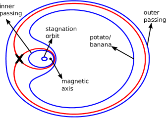
Figure 1: Schematic diagram of LAR characteristic orbits. Two separatrices, homoclinic to the x-point, are shown, each one acting as a boundary between two continents.

The conserved canonical momenta $P_{\chi}$ and $\mu$ are already the actions of the toroidal motion and the gyromotion respectively. The AA pair ($J,\theta$) of the poloidal motion is found by integrating along a closed orbit in the poloidal plane:

$$J\ =\ \frac{1}{2\pi}\oint P_{\tau}d\tau$$ (2)

and defining $\theta$ as the normalized time

$$\theta\ =\ \omega_{\theta}\left(J,P_{\chi},\mu\right)t,$$ (3)

where $\omega_{\theta}$ is the frequency of the poloidal motion and depends only on the three actions. By virtue of the Liouville–Arnlold theorem Ref. 34], such a transform always exists locally. In particular we can cover all phase space with a measurable set of AA transforms, one for each phase space region that is bounded by a separatrix. From now on we shall call such a region a continent, while the set of transforms for all regions is called an atlas.

Fig. 1 depicts a poloidal projection of LAR orbits with the same $P_{\chi}$ and $\mu$. Each of the two separatrices (thick red lines) separates two continents. All orbits belonging to the same continent share the same topology and the behaviour of the dynamics varies continuously within each continent. The conventional orbit labelling (e.g. passing, trapped, stagnated) is phenomenological and refers to the magnetic axis, because it is the natural reference point of the magnetic field geometry and very close to the natural reference point of the slow particle dynamics, i.e. the elliptic point of the inner passing orbits (first continent in the figure). However, for the energetic particle dynamics, the magnetic axis is not special from the dynamics point of view, and conventional labelling is arbitrary and confusing. For example, in Fig. 1, the two orbits marked as stagnation and inner passing orbits share the shame topology, but their conventional labelling is not the same. In fact, it would be more useful to label the orbits with respect to the continent they belong to. This choice not only underlines the dynamic characteristics of each orbit, but serves the purpose of clarity and algorithmic simplicity.

Although the Hamiltonian $H$ is integrable, finding an analytic solution is impractical. Instead, we calculate the atlas numerically. The algorithm we follow relies on finding the boundaries of each continent in $(\tau,\psi,P_{\chi},\mu)$ subspace, i.e. the separatrices, and then calculating numerically each AA transform defined by eqs. 2, 3 on a carefully chosen sample of closed orbits. The particulars of the algorithm will be discussed in another paper.

In transforming from $(\tau,\psi)$ to $(J,\theta)$, the angles of the other two DOFs are redefined, so that eventually all DOFs are described by AA pairs. In each continent, the transform is comprised from a non–canonical step, from $(\tau,\psi,P_{\chi},\mu)$ to $(\tau,P_{\tau},P_{\chi},\mu)$ (see Appendix), and a canonical one to $\left(\theta,J,P_{\chi},\mu\right)$, which is implicitly generated by a function of the form $F_{2}\ =\ F\left(\tau,J,P_{\chi},\mu\right)$. Dependence of $F_{2}$ on $P_{\chi}$ and $\mu$ implies that $\chi$ is also transformed to an angle variable

$$\hat{\chi}\ =\ \chi-f_{\chi}\left(J,\theta,P_{\chi},\mu\right)$$ (4)

and so does $\xi$. Therefore, this procedure generates the transform to the AA pairs $\left(P_{\chi},\hat{\chi}\right)$ and $\left(\mu,\bar{\xi}\right)$. The barred angles differ from the original in that they evolve linearly with time, with frequencies $\omega_{\hat{\chi}}$ and $\Omega_{c}$, which are the averaged drift frequency and the mean gyrofrequency respectively. By construction, the new poloidal angle $\theta$ evolves linearly as well, with the average poloidal frequency $\omega_{\theta}$, while the actions $J$, $P_{\chi}$ and $\mu$ are constants of motion.

III Chaotic Motion, Due To Nonresonant Magnetic Fields

We will demonstrate the power of the AA transform, by applying it on the study of the particle dynamics in the presence of nonresonant magnetic perturbations. As we show below, the particle motion can become chaotic, even though there is no destruction of the magnetic surfaces. This should come as no surprise, because, only only under the ZOW approximation is the chaoticity of the particle motion directly related to the chaoticity of the magnetic field lines. In this case, however, the drift effects are significant, so that the stochastisation of magnetic field lines is not a reliable criterion for predicting chaotic particle motion, when FOW effects are involved. Resonance and resonance overlap is a dynamic effect, the analysis of which, ideally, should be restricted on the particulars of phase space alone, without resorting to configuration geometry concepts. This is, of course, not the first time such a behaviour has been described (see, for example, Ref. 35] and references therein), but here it is analysed in the action space alone, without referring to the configuration geometry. The simplicity of this approach and the excellent quantitative results it can provide is a major advantage of the OSA method.

III.1 Orbital Spectrum Analysis

A perturbation of the form $\delta\mathbf{B}=\boldsymbol{\nabla}\times\sigma\mathbf{B}$ can be straightforwardly included in the guiding center Hamiltonian as $H=(\rho_{c}-\sigma)^{2}B^{2}/2+\mu B+\Phi$, $\rho_{c}=\rho_{\parallel}+\sigma$. Ref. 36] This introduces a first and second order perturbation Hamiltonian term. Any perturbation with physical meaning should be given in terms of the magnetic coordinates, or even the lab coordinates. The first order Hamiltonian $H_{1}$ is proportional to $\sigma$. Due to the nonlinear depencence of $\hat{\chi}$ on $\theta$ (eq. 4), a monochromatic mode $\sigma=A_{m,n}\left(\psi\right)\mathrm{exp}\left(i\left(m\chi+n\tau-\omega t\right)\right)$ in the magnetic coordinates gives an infinite series of modes in the AA phase space, so that

$$H_{1}=\sum_{s}{\mathcal{H}^{1}_{s,m}}\left(J,P_{\chi}\right)\ e^{i\left(m\hat{\chi}+s\theta-\omega t\right)},$$ (5)

where

$$\mathcal{H}^{1}_{s,m}\left(J,P_{\chi}\right)=\frac{1}{2\pi}\oint\limits_{J,P_{\chi}=\mathrm{const.}}H^{1}_{m,n}\left(\psi\right)\ e^{i\left(n\tau+nf_{\chi}\left(J,P_{\chi},\theta\right)-s\theta\right)}d\theta.$$ (6)

As equation eq. 5 indicates, the resonances of the perturbation are located in action space at the points where the resonance condition

$$m\ \omega_{\hat{\chi}}\left(J,P_{\chi},\mu\right)+s\ \omega_{\theta}\left(J,P_{\chi},\mu\right)-\omega\ =0$$ (7)

is met. The location of the resonances in action space depends only on the spectral parameters $m$ and $\omega$. The actual profile of the perturbation, i.e the depencence on $n$ or $\psi$, is relevant in defining the amplitude of the resonant terms, but not in pinpointing their location in the orbital spectrum. Since $s$ can take on any integer value, each bounded continent contains an infinite number of such frequencies, most of which are located in the narrow chaotic sea near the separatrix, where $\omega_{\theta}$ approaches zero. In the bulk of each continent there are only a few, if any, sites where eq. 7 is satisfied.

Near a particular resonance $m\ \omega_{\hat{\chi}}+s\ \omega_{\theta}-\omega=0$, the dynamics follow a pendulum– like Hamiltonian and a trapped area of width proportional to the square root of the perturbation amplitude is formed. The width depends on $\mathcal{H}_{s,m}\left(J,P_{\chi}\right)$ and can be easily calculated once the AA transform has been performed.

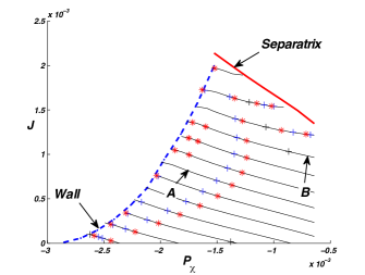
Figure 2: Resonance chart cross section in $\mu$. The solid black lines depict the energy surfaces, crosses and stars correspond to resonances with $m=10$ and $m=8$ respectively.

III.2 Application

We apply this analysis on the study of the dynamics in a peaked equilibrium (see Appendix) in the presence of two static magnetic perturbations with $m=8$ and $m=10$. The safety factor ranges from 1 to 1.8, so that the perturbations are nonresonant and no flux surface is destroyed. The amplitudes of the perturbation are of the order $\delta B/B\approx 10^{-4}-10^{-3}$, well inside the domain of validity of perturbation theory.

This case of time independent perturbations is particularly simple, but rather indicative of the power of the AA transform and the OSA method. The Hamiltonian is conserved and the quantity $P_{\chi}-m/sJ$ is an adiabatic invariant. The cases where the ratio $m/s$ or $s/m$ becomes very large are of little interest, since the adiabatic invariant coincides with one of the actions, so that no significant redistribution takes place.

Without any particular knowledge about the actual profile of the perturbations, other than the toroidal numbers, it is possible to chart the location of the resonances in the action space of each continent, by requiring that the condition

$$\frac{m\omega_{\hat{\chi}}}{\omega_{\theta}}\ =\ \textrm{integer}.$$ (8)

Fig. 2 depicts the chart of the $m=10$ and $m=8$ resonances in a potato–banana continent. The constant energy subsurfaces, on which the perturbed motion will be confined, due to time independence of the perturbation, are plotted with thick black lines.

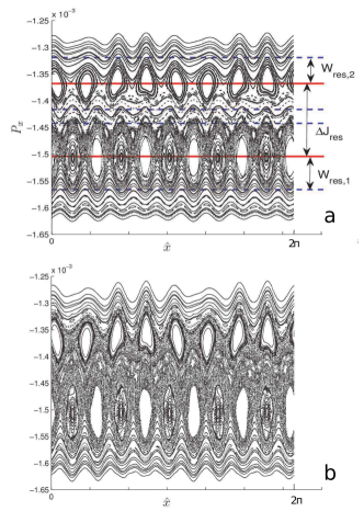
Figure 3: Inspection of the resonance chart can reveal the phase space regions when mode synergy can be significant. The analytically calculated resonance positions, width and overlap conditions are in excellent agreement with the simulations. a) Poincare plot on the surface A of Fig. 2 for two modes with subcritical amplitude. The semianalitically calculated positions of the resonances as well as their widths are denoted with solid and dashed lines respectively. b) The same Poincare plot for perturbations with critical amplitude. KAM lines between the two resonances have been destroyed and significant redistribution can take place.

Coexistence of more than one resonances on the same energy surface can lead to chaotic redistribution, due to destruction of the adiabatic invariant. On the energy surface denoted by A in Fig. 2 there are two neighbouring resonances located at $P_{\chi,1}\approx-1.5\cdot 10^{-3}$ and $P_{\chi,2}\approx-1.37\cdot 10^{-3}$. Chiricov criterion Ref. 20] provides a simple estimation for the onset of chaotic motion, by requiring that the resonances overlap. The resonance widths $W_{\textrm{res},i}$ are estimated by approximating the motion around the resonances with the pendulum Hamiltonian and using the well known formula for the separatrix width. The criterion requires that for chaotic motion

$$\Delta J\leq W_{\textrm{res},1}+W_{\textrm{res},2},$$ (9)

where $\Delta J$ is the distance between two neighbouring resonances.

As demonstrated in Fig. 3, the OSA method predicts both the location of the resonance center as well as the resonance width in the phase space. Moreover, application of the Chirikov criterion is shown very successful in predicting the transition from weak to strong chaos. Fig. 3a displays a Poincare plot of the perturbed motion, when the amplitude of the perturbation $A=A_{\textrm{subcrit}}$ is lower than the analytically computed critical amplitude $A_{\textrm{crit}}$. Some chaos is present, due to the existence of higher order resonances, but the primary resonances are well separated by KAM surfaces and no significant particle redistribution takes place. Superimposed on the Poincare plot are the analytically calculated locations of the resonances (solid lines) and the resonance widths (dashed lines). It is evident that the resonances do not overlap. The situation changes for $A=A_{\textrm{crit}}=A_{\textrm{Chiricov}}$ (Fig. 3b), for which the KAM surfaces have been destroyed and there is a chaotic sea between the two primary resonances. Some stickiness that can be observed a little lower than the upper chain of primary islands is reminiscent of the last KAM surface to be destroyed.

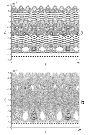
Figure 4: The OSA method as a tool for estimating conditions for confinement loss. The outer closed flux surface is marked with a thick dashed line. a) Poincare cut for the energy surface B of Fig. 2 and subcritical amplitude $0.08\ A_{\mathrm{Chirikov}}$. Only two of the resonances have partially overlapped. b) The same, with amplitude $0.3\ A_{\mathrm{Chirikov}}$. Although, this is still below the critical value determined by Chirikov criterion, the KAM surfaces have been destroyed. Chirikov criterion overestimates the critical amplitude, by ignoring higher order resonances.

The case of the energy surface B in Fig. 2 is of particular importance, because there is a line of resonances linking a deeply trapped part of phase space to the plasma wall (dashed blue line). Therefore, provided that all consecutive resonances overlap, significant particle loss can occur. Chirikov criterion determines the critical amplitude at $A_{\textrm{Chirikov}}=1.2\cdot 10^{-3}$,which is an overestimation of the critical amplitude $A_{\textrm{crit}}$, due to the strong presence of higher order resonances, as demonstrated in Fig. 4.

It is important to point out that zero orbit width approximations, which are necessary in order to calculate an analytical AA transform, cannot reproduce the picture described above. The location of the resonances is determined by requiring that $\omega_{\hat{\chi}}/\omega_{\theta}=s/10$ or $\omega_{\hat{\chi}}/\omega_{\theta}=s/8$, where $s$ is any integer. Figure 5 depicts the numerically calculated FOW frequency ratio curve, as well as the analytical one, calculated using well known formulas for ZOW approximation Ref. 36, 22]. As is clear from the figure, the two approaches predict entirely different resonance ratios and locations. ZOW approximation, therefore, fails for energetic particles, even in the case of a LAR equilibrium, where it is expected to be more accurate.

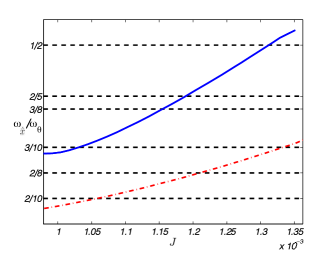
Figure 5: Toroidal over poloidal frequency ratio as a function of $J$ on the energy surface B. The resonances with the $m=8$ and $m=10$ are located at the intersections with the horizontal dashed lines. Solid curve: numerical calculation with full orbit width effects. Dashed-dotted curve: analytic zero orbit width approximation.

The previous analysis refers to the phase space study of the single particle motion. The resulting kinetic modelling of the collective dynamical behaviour consists of a Focker–Plank equation for the evolution of the Angle-averaged distribution function in the Action space, when the transition to strong chaos has occurred Ref. 20, 37]. The three Action variables are related to magnetic moment, parallel momentum and radial position (or energy) so that particle, momentum and energy transport is described by the corresponding Action-dependent quasilinear diffusion tensor.

Assuming that the gyromotion is much faster than every other process involved, the magnetic moment remains constant and the resonance condition Eq. 7, which does not involve the gyrofrequency $\Omega_{c}$, applies Ref. 9]. At the points where the resonance condition is met, the diffusion tensor is given by

$$\boldsymbol{\bar{D}}=\pi\sum\limits_{\mathbf{r}}\mathbf{r}\mathbf{r}\left|\mathcal{H}^{1}_{\mathbf{r}}\right|^{2}\delta(\mathbf{r}\cdot\boldsymbol{\omega}),$$ (10)

and the Focker–Plank equation takes the form

$$\frac{\partial}{\partial t}f\left(\boldsymbol{I},\mu;t\right)\ =\ \frac{\partial}{\partial\boldsymbol{I}}\cdot\left(\boldsymbol{D}\cdot\frac{\partial}{\partial\boldsymbol{I}}f\left(\boldsymbol{I},\mu;t\right)\right)$$ (11)

where $\mathbf{r}=(s,m)$ is the vector of the harmonic numbers, $\boldsymbol{\omega}=(\omega_{\theta},\omega_{\hat{\chi}})$, $\boldsymbol{I}=(J,P_{\chi})$ and $f$ is the distribution function Ref. 37, 38]. The diffusion tensor $\boldsymbol{D}$ used in the Focker–Plank equation is a smooth function that interpolates the singular diffusion tensor $\boldsymbol{\bar{D}}$ at the resonance points. This is because of the spreading of resonances, due to nonlinear effects Ref. 9]. The fact that the diffusion tensor can be expressed explicitly in Action space is one of the many advantages of the AA formalism. Fig. 6 depicts the $J,J$ element of the diffusion tensor as a function of $J$ for the case of Fig. 4b.

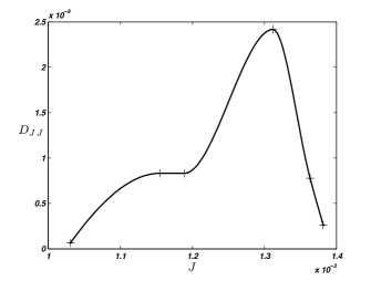
Figure 6: The $J,J$ element of the quasilinear tensor for the case of Fig. 4b.

IV Summary and Conclusions

The Orbital Spectrum Analysis (OSA) method of any type of non-axisymmetric pertirbation on the GC motion has been presented. The method is based on the Action-Angle (AA) transform of the unperturbed motion allowing for the calculation of the orbital frequencies of the three degrees of freedom and the explicit expression of the resonant conditions as well as of the perturbations in AA variables. It is shown that the exact location and the strength (width) of the resonances in the GC phase space can be calculated, providing an apriori knowledge (without tracing particles) of the effect perturbations including synegetic effects between different types of perturbations. It is worthmentioning that the AA transform is determined from each specific axisymmetric equilibrium and completely characterizes it in terms of the GC motion. Therefore, it has to be calculated only once for a given equilibrium and then it is available for the orbital spectrum analysis of any perturbation. The OSA method serves as an ideal tool for phase space engineering of the synergetic of antagonistic effects of different types of perturbations.

*

Appendix A Flux coordinates

The White–Boozer notation is summarised Ref. 36]. In a nested flux surface magnetic field configuration the magnetic field can be represented as

$$\boldsymbol{B}\ =\boldsymbol{\nabla}\psi\times\boldsymbol{\nabla}\theta+\boldsymbol{\nabla}\zeta\times\boldsymbol{\nabla}\psi_{p},$$ (12)

where $\theta$ is the poloidal angle, $\psi$ is the toroidal flux variable, $\psi_{p}(\psi)$ is the poloidal flux variable. This is the contravariant representation of the field. The covariant representation is given by

$$\boldsymbol{B}\ =\hat{\delta}\left(\psi,\theta,\zeta\right)\boldsymbol{\nabla}\psi+\hat{I}\left(\psi,\theta,\zeta\right)\boldsymbol{\nabla}\theta+\hat{g}\left(\psi,\theta,\zeta\right)\boldsymbol{\nabla}\zeta.$$ (13)

There is always a transform of the angular variables $\theta,\zeta$ to the variables $\tau,\chi$ so that the Jacobian $\mathcal{J}$ of the new system $(\psi,\tau,\chi)$ satisfies $\mathcal{J}=f(\psi)/B^{2}$. This is the Boozer representation Ref. 39]. The covariant representation then becomes

$$\boldsymbol{B}\ ={\delta}\left(\psi,\theta,\zeta\right)\boldsymbol{\nabla}\psi+{I}\left(\psi\right)\boldsymbol{\nabla}\tau+{g}\left(\psi\right)\boldsymbol{\nabla}\chi.$$ (14)

In this representation, the equations of motion are canonical. The canonical momenta conjugate to $\tau,\chi$ are

$$P_{\tau}\equiv\psi+\rho_{\parallel}I$$ (15)

and

$$P_{\chi}\equiv\rho_{\parallel}g+\psi_{p}$$ (16)

respectively. The Hamiltonian in eq. 1 takes the form

$$H=\frac{\left(P_{\chi}+\psi_{p}\left(P_{\tau},P_{\chi}\right)\right)^{2}}{2g^{2}\left(P_{\tau},P_{\chi}\right)}B^{2}+\mu B+\Phi,$$ (17)

When $B$ and $\Phi$ are independent of the generalized toroidal angle $\chi$ (quasisymmetric configuration), $P_{\chi}$ is a constant of motion.

The safety factor, defined as $q=\boldsymbol{B}\cdot\boldsymbol{\nabla}\chi/\boldsymbol{B}\cdot\boldsymbol{\nabla}\tau$, is determined by the balance of the pressure and the magnetic force and, as its name suggests, its profile is an important characteristic of the equilibrium. It is a flux function in Boozer coordinates. It is known that, for LAR equilibria, q profiles of the form

$$q=q_{0}\left(1+\left(\psi/\psi_{0}\right)^{\nu}\right)^{\frac{1}{\nu}}$$ (18)

are acceptable solutions of the force balance condition. Equilibria with $\nu=1,2,3$ are referred to as peaked, rounded and flat respectively Ref. 36].

References

- Cary and Brizard Ref. 2009] J. R. Cary and A. J. Brizard. Hamiltonian theory of guiding-center motion. Rev. Mod. Phys., 81:693, May 2009.
- Littlejohn Ref. 1979] R. G. Littlejohn. A guiding center hamiltonian: A new approach. J. Math. Phys., 20(12):2445, 1979.
- White and Chance Ref. 1984] R. B. White and M. S. Chance. Hamiltonian guiding center drift orbit calculation for plasmas of arbitrary cross section. Phys. Fluids, 27(10), 1984.
- Goldstein Ref. 1956] H. Goldstein. Classical mechanics. Cambridge: Addison-Wesley, 1956.
- Littlejohn Ref. 1983] R. G. Littlejohn. Variational principles of guiding centre motion. J. Plasma Phys., 29, 2 1983.
- White et al. Ref. 2010] R. B. White, N. Gorelenkov, W. W. Heidbrink, and M. A. Van Zeeland. Particle distribution modification by low amplitude modes. Plasma Phys. Controlled Fusion, 52(4):045012, 2010.
- White Ref. 2012] R. B. White. Modification of particle distributions by mhdinstabilities i. Commun. Nonlinear Sci., 17(5):2200, 2012.
- Brizard and Hahm Ref. 2007] A. J. Brizard and T. S. Hahm. Foundations of nonlinear gyrokinetic theory. Rev. Mod. Phys., 79:421–468, Apr 2007.
- Kaufman Ref. 1972a] A. N. Kaufman. Quasilinear diffusion of an axisymmetric toroidal plasma. Phys. Fluids, 15(6):1063, 1972a.
- Lamalle Ref. 1993] P.U. Lamalle. The nonlocal radio-frequency response of a toroidal plasma. Phys. Lett. A, 175(1):45–52, 1993.
- Eester and Koch Ref. 1998] D. Van Eester and R. Koch. A variational principle for studying fast-wave mode conversion. Plasma Phys. Controlled Fusion, 40(11):1949, 1998.
- Brambilla Ref. 1999] M. Brambilla. Numerical simulation of ion cyclotron waves in tokamak plasmas. Plasma Phys. Controlled Fusion, 41(1):1, 1999.
- White et al. Ref. 1982] R. B. White, A. H. Boozer, and R. Hay. Drift hamiltonian in magnetic coordinates. Phys. Fluids, 25(3), 1982.
- Wang Ref. 2006] S. Wang. Canonical hamiltonian theory of the guiding-center motion in an axisymmetric torus, with the different time scales well separated. Phys. Plasmas, 13(5), 2006.
- Hazeltine et al. Ref. 1981] R. D. Hazeltine, S. M. Mahajan, and D. A. Hitchcock. Quasilinear diffusion and radial transport in tokamaks. Phys. Fluids, 24(6), 1981.
- Gambier and Samain Ref. 1985] D. J. Gambier and A. Samain. Variational theory of ion cyclotron resonance heating in tokamak plasmas. Nucl. Fusion, 25(3):283, 1985.
- Kominis et al. Ref. 2008] Y. Kominis, A. K. Ram, and K. Hizanidis. Quasilinear theory of electron transport by radio frequency waves and nonaxisymmetric perturbations in toroidal plasmas. Phys. Plasmas, 15(12), 2008.
- Kominis Ref. 2008] Y. Kominis. Nonlinear theory of cyclotron resonant wave-particle interactions: Analytical results beyond the quasilinear approximation. Phys. Rev. E, 77:016404, Jan 2008.
- Kominis et al. Ref. 2010] Y. Kominis, A. K. Ram, and K. Hizanidis. Kinetic theory for distribution functions of wave-particle interactions in plasmas. Phys. Rev. Lett., 104:235001, 2010.
- Lichtenberg and Lieberman Ref. 1992] A. J. Lichtenberg and M. A. Lieberman. Regular and Chaotic Dynamics, volume 38 of Applied Mathematical Sciences. Springer–Verlag, 1992.
- Abdullaev et al. Ref. 2006] S. S. Abdullaev, A. Wingen, and K. H. Spatschek. Mapping of drift surfaces in toroidal systems with chaotic magnetic fields. Phys. Plasmas, 13(4), 2006.
- Brizard Ref. 2011] A. J. Brizard. Compact formulas for guiding-center orbits in axisymmetric tokamak geometry. Phys. Plasmas, 18(2), 2011.
- Gott and Yurchenko Ref. 2014] Y. V. Gott and E. I. Yurchenko. Topology of drift trajectories of charged particles in a tokamak. Plasma Phys. Rep., 40(4), 2014.
- Eriksson and Porcelli Ref. 2001] L. G. Eriksson and F. Porcelli. Dynamics of energetic ion orbits in magnetically confined plasmas. Plasma Phys. Controlled Fusion, 43(4), 2001.
- Bergmann et al. Ref. 2001] A. Bergmann, A. G. Peeters, and S. D. Pinches. Guiding center particle simulation of wide-orbit neoclassical transport. Phys. Plasmas, 8(12):5192, 2001.
- Lin et al. Ref. 1997] Z. Lin, W. M. Tang, and W. W. Lee. Large orbit neoclassical transport. Phys. Plasmas, 4(5):1707, 1997.
- Shaing et al. Ref. 1997] K. C. Shaing, R. D. Hazeltine, and M. C. Zarnstorff. Ion transport process around magnetic axis in tokamaks. Phys. Plasmas, 4(3):771, 1997.
- Shaing and Peng Ref. 2004] K. C. Shaing and M. Peng. Transport theory for potato orbits in an axisymmetric torus with finite toroidal flow speed. Phys. Plasmas, 11(8):3726–3732, 2004.
- Helander Ref. 2000] P. Helander. On neoclassical transport near the magnetic axis. Phys. Plasmas, 7(7):2878, 2000.
- Chen Ref. 2013] F.F. Chen. Introduction to Plasma Physics and Controlled Fusion: Volume 1: Plasma Physics. Springer Science & Business Media, 2013.
- Wesson Ref. 2004] J. Wesson. Tokamaks. Oxford University, 2004.
- Eester Ref. 1999] D. Van Eester. Trajectory integral and hamiltonian descriptions of radio frequency heating in tokamaks. Plasma Phys. Controlled Fusion, 41(7):L23, 1999.
- Troia Ref. 2012] C. Di Troia. From the orbit theory to a guiding center parametric equilibrium distribution function. Plasma Phys. Controlled Fusion, 54(10):105017, 2012.
- Arnold Ref. 1989] V. I. Arnold. Mathematical methods of classical mechanics. Springer-Verlag, New York, 1989.
- Matsuyama et al. Ref. 2014] A. Matsuyama, M. Yagi, Y. Kagei, and N. Nakajima. Drift resonance effect on stochastic runaway electron orbit in the presence of low-order magnetic perturbations. Nucl. Fusion, 54(12):123007, 2014.
- White Ref. 2001] R. B. White. The theory of toroidally confined plasmas. Imperial College Press, 2001.
- Kaufman Ref. 1972b] A. N. Kaufman. Reformulation of quasi-linear theory. J. Plasma Phys., 8:1, 8 1972b.
- Abdullaev Ref. 2006] S. S. Abdullaev. Construction of mappings for Hamiltonian systems and their applications, volume 691 of Lecture Notes in Physics. Springer, 2006.
- Boozer Ref. 1980] A. H. Boozer. Guiding center drift equations. Phys. Fluids, 23(5):904, 1980.