Dynamic Capacity Networks
Abstract
We introduce the Dynamic Capacity Network (DCN), a neural network that can adaptively assign its capacity across different portions of the input data. This is achieved by combining modules of two types: low-capacity sub-networks and high-capacity sub-networks. The low-capacity sub-networks are applied across most of the input, but also provide a guide to select a few portions of the input on which to apply the high-capacity sub-networks. The selection is made using a novel gradient-based attention mechanism, that efficiently identifies input regions for which the DCN’s output is most sensitive and to which we should devote more capacity. We focus our empirical evaluation on the Cluttered MNIST and SVHN image datasets. Our findings indicate that DCNs are able to drastically reduce the number of computations, compared to traditional convolutional neural networks, while maintaining similar or even better performance.
capbtabboxtable[][\FBwidth]
1 Introduction
Deep neural networks have recently exhibited state-of-the-art performance across a wide range of tasks, including object recognition (Szegedy et al., 2014) and speech recognition (Graves & Jaitly, 2014). Top-performing systems, however, are based on very deep and wide networks that are computationally intensive. One underlying assumption of many deep models is that all input regions contain the same amount of information. Indeed, convolutional neural networks apply the same set of filters uniformly across the spatial input (Szegedy et al., 2014), while recurrent neural networks apply the same transformation at every time step (Graves & Jaitly, 2014). Those networks lead to time-consuming training and inference (prediction), in large part because they require a large number of weight/activation multiplications.
Task-relevant information, however, is often not uniformly distributed across input data. For example, objects in images are spatially localized, i.e. they exist only in specific regions of the image. This observation has been exploited in attention-based systems (Mnih et al., 2014), which can reduce computations significantly by learning to selectively focus or “attend” to few, task-relevant, input regions. Attention employed in such systems is often referred to as “hard-attention”, as opposed to “soft-attention” which integrates smoothly all input regions. Models of hard-attention proposed so far, however, require defining an explicit predictive model, whose training can pose challenges due to its non-differentiable cost.
In this work we introduce the Dynamic Capacity Network (DCN) that can adaptively assign its capacity across different portions of the input, using a gradient-based hard-attention process. The DCN combines two types of modules: small, low-capacity, sub-networks, and large, high-capacity, sub-networks. The low-capacity sub-networks are active on the whole input, but are used to direct the high-capacity sub-networks, via our attention mechanism, to task-relevant regions of the input.
A key property of the DCN’s hard-attention mechanism is that it does not require a policy network trained by reinforcement learning. Instead, we can train DCNs end-to-end with backpropagation. We evaluate a DCN model on the attention benchmark task Cluttered MNIST (Mnih et al., 2014), and show that it outperforms the state of the art.
In addition, we show that the DCN’s attention mechanism can deal with situations where it is difficult to learn a task-specific attention policy due to the lack of appropriate data. This is often the case when training data is mostly canonicalized, while at test-time the system is effectively required to perform transfer learning and deal with substantially different, noisy real-world images. The Street View House Numbers (SVHN) dataset (Netzer et al., 2011) is an example of such a dataset. The task here is to recognize multi-digit sequences from real-world pictures of house fronts; however, most digit sequences in training images are well-centred and tightly cropped, while digit sequences of test images are surrounded by large and cluttered backgrounds. Learning an attention policy that focuses only on a small portion of the input can be challenging in this case, unless test images are pre-processed to deal with this discrepancy 111This is the common practice in previous work on this dataset, e.g. (Goodfellow et al., 2013; Ba et al., 2014; Jaderberg et al., 2015). DCNs, on the other hand, can be leveraged in such transfer learning scenarios, where we learn low and high capacity modules independently and only combine them using our attention mechanism at test-time. In particular, we show that a DCN model is able to efficiently recognize multi-digit sequences, directly from the original images, without using any prior information on the location of the digits.
Finally, we show that DCNs can perform efficient region selection, in both Cluttered MNIST and SVHN, which leads to significant computational advantages over standard convolutional models.
2 Dynamic Capacity Networks
In this section, we describe the Dynamic Capacity Network (DCN) that dynamically distributes its network capacity across an input.
We consider a deep neural network , which we decompose into two parts: where and represent respectively the bottom layers and top layers of the network while is some input data. Bottom layers operate directly on the input and output a representation, which is composed of a collection of vectors each of which represents a region in the input. For example, can output a feature map, i.e. vectors of features each with a specific spatial location, or a probability map outputting probability distributions at each different spatial location. Top layers consider as input the bottom layers’ representations and output a distribution over labels.
DCN introduces the use of two alternative sub-networks for the bottom layers : the coarse layers or the fine layers , which differ in their capacity. The fine layers correspond to a high-capacity sub-network which has a high-computational requirement, while the coarse layers constitute a low-capacity sub-network. Consider applying the top layers only on the fine representation, i.e. . We refer to the composition as the fine model. We assume that the fine model can achieve very good performance, but is computationally expensive. Alternatively, consider applying the top layers only on the coarse representation, i.e. . We refer to this composition as the coarse model. Conceptually, the coarse model can be much more computationally efficient, but is expected to have worse performance than the fine model.
The key idea behind DCN is to have use representations from either the coarse or fine layers in an adaptive, dynamic way. Specifically, we apply the coarse layers on the whole input , and leverage the fine layers only at a few “important” input regions. This way, the DCN can leverage the capacity of , but at a lower computational cost, by applying the fine layers only on a small portion of the input. To achieve this, DCN requires an attentional mechanism, whose task is to identify good input locations on which to apply . In the remainder of this section, we focus on 2-dimensional inputs. However, our DCN model can be easily extended to be applied to any type of N-dimensional data.
2.1 Attention-based Inference

In DCN, we would like to obtain better predictions than those made by the coarse model while keeping the computational requirement reasonable. This can be done by selecting a few salient input regions on which we use the fine representations instead of the coarse ones. DCN inference therefore needs to identify the important regions in the input with respect to the task at hand. For this, we use a novel approach for attention that uses backpropagation in the coarse model to identify few vectors in the coarse representation to which the distribution over the class label is most sensitive. These vectors correspond to input regions which we identify as salient or task-relevant.
Given an input image , we first apply the coarse layers on all input regions to compute the coarse representation vectors:
| (1) |
where and are spatial dimensions that depend on the image size and is a representation vector associated with the input region in , i.e. corresponds to a specific receptive field or a patch in the input image. We then compute the output of the model based completely on the coarse vectors, i.e. the coarse model’s output .
Next, we identify a few salient input regions using an attentional mechanism that exploits a saliency map generated using the coarse model’s output. The specific measure of saliency we choose is based on the entropy of the coarse model’s output, defined as:
| (2) |
where is the vector output of the coarse model and is the number of class labels. The saliency of an input region position is given by the norm of the gradient of the entropy with respect to the coarse vector :
| (3) | ||||
where . The use of the entropy gradient as a saliency measure encourages selecting input regions that could affect the uncertainty in the model’s predictions the most. In addition, computing the entropy of the output distribution does not require observing the true label, hence the measure is available at inference time. Note that computing all entries in matrix can be done using a single backward pass of backpropagation through the top layers and is thus efficient and simple to implement.
Using the saliency map , we select a set of input region positions with the highest saliency values. We denote the selected set of positions by , such that . We denote the set of selected input regions by where each is a patch in . Next we apply the fine layers only on the selected patches and obtain a small set of fine representation vectors:
| (4) |
where . This requires that , i.e. the fine vectors have the same dimensionality as the coarse vectors, allowing the model to use both of them interchangeably.
We denote the representation resulting from combining vectors from both and as the refined representation . We discuss in Section 4 different ways in which they can be combined in practice. Finally, the DCN output is obtained by feeding the refined representation into the top layers, . We denote the composition by the refined model.
2.2 End-to-End Training
In this section, we describe an end-to-end procedure for training the DCN model that leverages our attention mechanism to learn and jointly. We emphasize, however, that DCN modules can be trained independently, by training a coarse and a fine model independently and combining them only at test-time using our attention based inference. In Section 4.2 we show an example of how this modular training can be used for transfer learning.
In the context of image classification, suppose we have a training set , where each is an image, and is its corresponding label. We denote the parameters of the coarse, fine and top layers by , , and respectively. We learn all of these parameters (denoted as ) by minimizing the cross-entropy objective function (which is equivalent to maximizing the log-likelihood of the correct labels):
| (5) |
where is the conditional multinomial distribution defined over the labels given by the refined model (Figure 1). Gradients are computed by standard back-propagation through the refined model, i.e. propagating gradients at each position into either the coarse or fine features, depending on which was used.
An important aspect of the DCN model is that the final prediction is based on combining representations from two different sets of layers, namely the coarse layers and the fine layers . Intuitively, we would like those representations to have close values such that they can be interchangeable. This is important for two reasons. First, we expect the top layers to have more success in correctly classifying the input if the transition from coarse to fine representations is smooth. The second is that, since the saliency map is based on the gradient at the coarse representation values and since the gradient is a local measure of variation, it is less likely to reflect the benefit of using the fine features if the latter is very different from the former.
To encourage similarity between the coarse and fine representations while training, we use a hint-based training approach inspired by Romero et al. (2014). Specifically, we add an additional term to the training objective that minimizes the squared distance between coarse and fine representations:
| (6) |
There are two important points to note here. First, we use this term to optimize only the coarse layers . That is, we encourage the coarse layers to mimic the fine ones, and let the fine layers focus only on the signal coming from the top layers. Secondly, computing the above hint objective over representations at all positions would be as expensive as computing the full fine model; therefore, we encourage in this term similarity only over the selected salient patches.
3 Related Work
This work can be classified as a conditional computation approach. The goal of conditional computation, as put forward by Bengio (2013), is to train very large models for the same computational cost as smaller ones, by avoiding certain computation paths depending on the input. There have been several contributions in this direction. Bengio et al. (2013) use stochastic neurons as gating units that activate specific parts of a neural network. Our approach, on the other hand, uses a hard-attention mechanism that helps the model to focus its computationally expensive paths only on important input regions, which helps in both scaling to larger effective models and larger input sizes.
Several recent contributions use attention mechanisms to capture visual structure with biologically inspired, foveation-like methods, e.g. (Larochelle & Hinton, 2010; Denil et al., 2012; Ranzato, 2014; Mnih et al., 2014; Ba et al., 2014; Gregor et al., 2015). In Mnih et al. (2014); Ba et al. (2014), a learned sequential attention model is used to make a hard decision as to where to look in the image, i.e. which region of the image is considered in each time step. This so-called “hard-attention” mechanism can reduce computation for inference. The attention mechanism is trained by reinforcement learning using policy search. In practice, this approach can be computationally expensive during training, due to the need to sample multiple interaction sequences with the environment. On the other hand, the DRAW model (Gregor et al., 2015) uses a “soft-attention” mechanism that is fully differentiable, but requires processing the whole input at each time step. Our approach provides a simpler hard-attention mechanism with computational advantages in both inference and learning.
The saliency measure employed by DCN’s attention mechanism is related to pixel-wise saliency measures used in visualizing neural networks (Simonyan et al., 2013). These measures, however, are based on the gradient of the classification loss, which is not applicable at test-time. Moreover, our saliency measure is defined over contiguous regions of the input rather than on individual pixels. It is also task-dependent, as a result of defining it using a coarse model trained on the same task.
Other works such as matrix factorization (Jaderberg et al., 2014; Denton et al., 2014) and quantization schemes (Chen et al., 2010; Jégou et al., 2011; Gong et al., 2014) take the same computational shortcuts for all instances of the data. In contrast, the shortcuts taken by DCN specialize to the input, avoiding costly computation except where needed. However, the two approaches are orthogonal and could be combined to yield further savings.
Our use of a regression cost for enforcing representations to be similar is related to previous work on model compression (Buciluǎ et al., 2006; Hinton et al., 2015; Romero et al., 2014). The goal of model compression is to train a small model (which is faster in deployment) to imitate a much larger model or an ensemble of models. Furthermore, Romero et al. (2014) have shown that middle layer hints can improve learning in deep and thin neural networks. Our DCN model can be interpreted as performing model compression on the fly, without the need to train a large model up front.
4 Experiments
In this section, we present an experimental evaluation of the proposed DCN model. To validate the effectiveness of our approach, we first investigate the Cluttered MNIST dataset (Mnih et al., 2014). We then apply our model in a transfer learning setting to a real-world object recognition task using the Street View House Numbers (SVHN) dataset (Netzer et al., 2011).
4.1 Cluttered MNIST
We use the Cluttered MNIST digit classification dataset (Mnih et al., 2014). Each image in this dataset is a hand-written MNIST digit located randomly on a black canvas and cluttered with digit-like fragments. Therefore, the dataset has the same size of MNIST: 60000 images for training and 10000 for testing.
4.1.1 Model Specification
In this experiment we train a DCN model end-to-end, where we learn coarse and fine layers jointly. We use 2 convolutional layers as coarse layers, 5 convolutional layers as fine layers and one convolutional layer followed by global max pooling and a softmax as the top layers. Details of their architectures can be found in the Appendix 6.1. The coarse and fine layers produce feature maps, i.e. feature vectors each with a specific spatial location. The set of selected patches is composed of eight patches of size pixels. We use here a refined representation of the full input in which fine feature vectors are swapped in place of coarse ones:
| (7) | |||||
| (8) |
4.1.2 Baselines
4.1.3 Empirical Evaluation
| Model | Test Error |
|---|---|
| RAM | 8.11% |
| DRAW | 3.36% |
| Coarse Model | 3.69% |
| Fine Model | 1.70% |
| DCN w/o hints | 1.71% |
| DCN with hints | 1.39% |

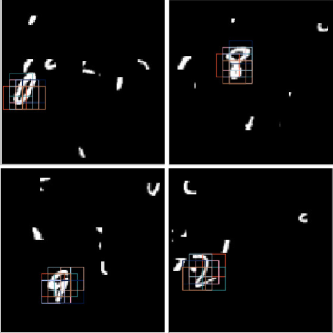
Results of our experiments are shown in Table 1. We get our best DCN result when we add the hint term in Eq. (6) in the training objective, which we observe to have a regularization effect on DCN. We can see that the DCN model performs significantly better than the previous state-of-the-art result achieved by RAM and DRAW models. It also outperforms the fine model, which is a result of being able to focus only on the digit and ignore clutter. In Figure 2 we explore more the effect of the hint objective during training, and confirm that it can indeed minimize the squared distance between coarse and fine representations. To show how the attention mechanism of the DCN model can help it focus on the digit, we plot in Figure 3 the patches it finds in some images from the validation set, after only 9 epochs of training.
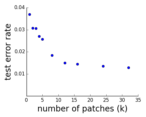
The DCN model is also more computationally efficient. A forward pass of the fine model requires the computation of the fine layers representations on whole inputs and a forward pass of the top layers leading to 84.5M multiplications. On the other hand, DCN applies only the coarse layers on the whole input. It also requires the computation of the fine representations for 8 input patches and a forward pass of the top layers. The attention mechanism of the DCN model requires an additional forward and backward pass through the top layers which leads to approximately M multiplications in total. As a result, the DCN model here has 3 times fewer multiplications than the fine model. In practice we observed a time speed-up by a factor of about 2.9. Figure 3 shows how the test error behaves when we increase the number of patches. While taking additional patches improves accuracy, the marginal improvement becomes insignificant beyond 10 or so patches. The number of patches effectively controls a trade-off between accuracy and computational cost.
4.2 SVHN
We tackle in this section a more challenging task of transcribing multi-digit sequences from natural images using the Street View House Numbers (SVHN) dataset (Netzer et al., 2011). SVHN is composed of real-world pictures containing house numbers and taken from house fronts. The task is to recognize the full digit sequence corresponding to a house number, which can be of length 1 to 5 digits. The dataset has three subsets: train (33k), extra (202k) and test (13k). In the following, we trained our models on 230k images from both the train and extra subsets, where we take a 5k random sample as a validation set for choosing hyper-parameters.
The typical experimental setting in previous literature, e.g. (Goodfellow et al., 2013; Ba et al., 2014; Jaderberg et al., 2015), uses the location of digit bounding boxes as extra information. Input images are generally cropped, such that digit sequences are centred and most of the background and clutter information is pruned. We argue that our DCN model can deal effectively with real-world noisy images having large portions of clutter or background information. To demonstrate this ability, we investigate a more general problem setting where the images are uncropped and the digits locations are unknown. We apply our models on SVHN images in their original sizes and we do not use any extra bounding box information. 222The only pre-processing we perform on the data is converting images to grayscale.
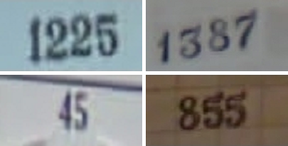
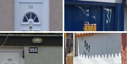
An important property of the SVHN dataset is the large discrepancy between the train/extra sets and the test set. Most of the extra subset images (which dominate the training data) have their digits well-centred with little cluttered background, while test images have more variety in terms of digit location and background clutter. Figure 4 shows samples of these images. We can tackle this training/test dataset discrepancy by training a DCN model in a transfer learning setting. We train the coarse and fine layers of the DCN independently on the training images that have little background-clutter, and then combine them using our attention mechanism, which does not require explicit training, to decide on which subsets of the input to apply the fine layers.
4.2.1 Multi-Digit Recognition Model
We follow the model proposed in (Goodfellow et al., 2013) for learning a probabilistic model of the digit sequence given an input image . The output sequence is defined using a collection of random variables, , representing the elements of the sequence and an extra random variable representing its length. The probability of a given sequence is given by:
| (9) |
where is the conditional distribution of the sequence length and is the conditional distribution of the -th digit in the sequence. In particular, our model on SVHN has 6 softmaxes: 1 for the length of the sequence (from to ), and 5 for the identity of each digit or a null character if no digit is present (11 categories).
4.2.2 Model Specification
The coarse and fine bottom layers, and , are fully-convolutional, composed of respectively and layers. The representation, produced by either the fine or coarse layers, is a probability map, which is a collection of independent full-sequence prediction vectors, each vector corresponding to a specific region of the input. We denote the prediction for the -th output at position by .
The top layer is composed of one global average pooling layer which combines predictions from various spatial locations to produce the final prediction .
Since we have multiple outputs in this task, we modify the saliency measure used by the DCN’s attention mechanism to be the sum of the entropy of the 5 digit softmaxes:
| (10) |
When constructing the saliency, instead of using the gradient with respect to the probability map, we use the gradient with respect to the feature map below it. This is necessary to avoid identical gradients as , the top function, is composed by only one average pooling.
We also use a refined model that computes its output by applying the pooling top layer only on the independent predictions from fine layers, ignoring the coarse layers. We have found empirically that this results in a better model, and suspect that otherwise the predictions from the salient regions are drowned out by the noisy predictions from uninformative regions.
We train the coarse and fine layers of DCN independently in this experiment, minimizing using SGD. For the purposes of training only, we resize images to . Details on the coarse and fine architectures are found in Appendix 6.2.
4.2.3 Baselines
As mentioned in the previous section, each of the coarse representation vectors in this experiment corresponds to multi-digit recognition probabilities computed at a given region, which the top layer simply averages to obtain the baseline coarse model:
| (11) |
The baseline fine model is defined similarly.
As an additional baseline, we consider a “soft-attention” coarse model, which takes the coarse representation vectors over all input regions, but uses a top layer that performs a weighted average of the resulting location-specific predictions. We leverage the entropy to define a weighting scheme which emphasizes important locations:
| (12) |
The weight is defined as the normalized inverse entropy of the -th prediction by the -th vector, i.e. :
| (13) |
where is defined as:
| (14) |
and is either for or for all other . As we’ll see, this weighting improves the coarse model’s performance in our SVHN experiments. We incorporate this weighting in DCN to aggregate predictions from the salient regions.
To address scale variations in the data, we extend all models to multi-scale by processing each image several times at multiple resolutions. Predictions made at different scales are considered independent and averaged to produce the final prediction.
It is worth noting that all previous literature on SVHN dealt with a simpler task where images are cropped and resized. In this experiment we deal with a more general setting, and our results cannot be directly compared with these results.
| Model | Test Error |
|---|---|
| Coarse model, 1 scale | 40.6% |
| Coarse model, 2 scales | 40.0% |
| Coarse model, 3 scales | 40.0% |
| Fine model, 1 scale | 25.2% |
| Fine model, 2 scales | 23.7% |
| Fine model, 3 scales | 23.3% |
| Soft-attention, 1 scale | 31.4% |
| Soft-attention, 2 scales | 31.1% |
| Soft-attention, 3 scales | 30.8% |
| DCN, 6 patches, 1 scale | 20.0% |
| DCN, 6 patches, 2 scales | 18.2% |
| DCN, 9 patches, 3 scales | 16.6% |
4.2.4 Empirical Evaluation
Table 2 shows results of our experiment on SVHN. The coarse model has an error rate of , while by using our proposed soft-attention mechanism, we decrease the error rate to . This confirms that the entropy is a good measure for identifying important regions when task-relevant information is not uniformly distributed across input data.
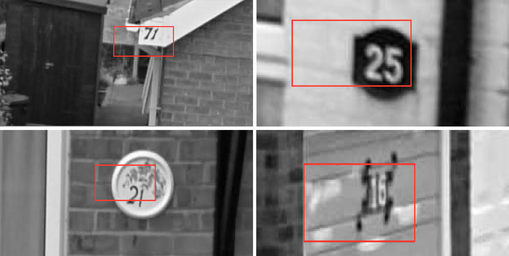
The fine model, on the other hand, achieves a better error rate of , but is more computationally expensive. Our DCN model, which selects only 6 regions on which to apply the high-capacity fine layers, achieves an error rate of . The DCN model can therefore outperform, in terms of classification accuracy, the other baselines. This verifies our assumption that by applying high capacity sub-networks only on the input’s most informative regions, we are able to obtain high classification performance. Figure 6 shows a sample of the selected patches by our attention mechanism.
An additional decrease of the test errors can be obtained by increasing the number of processed scales. In the DCN model, taking 3 patches at 2 scales (original and 0.75 scales), leads to error, while taking 3 patches at 3 scales (original, 0.75 and 0.5 scales) leads to an error rate of . Our DCN model can reach its best performance of by taking all possible patches at 3 scales, but it does not offer any computational benefit over the fine model.
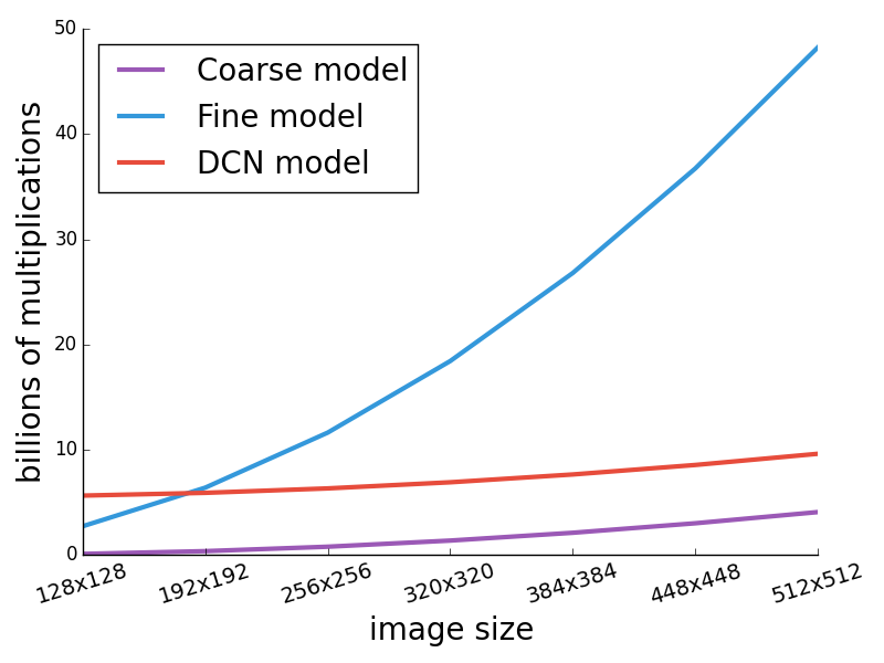
We also investigate the computational benefits of the DCN approach as the dimensions of the input data increase. Table 5 reports the number of multiplications the fine model, coarse model and the DCN model require, given different input sizes. We also verify the actual computational time of these models by taking the largest 100 images in the SVHN test set, and computing the average inference time taken by all the models. 333We evaluate all models on an NVIDIA Titan Black GPU card. The smallest of these images has a size of pixels, while the largest has a size of pixels. On average, the coarse and the soft-attention models take milliseconds, while the fine model takes milliseconds. On the largest 100 SVHN test images, the DCN requires on average milliseconds for inference.
5 Conclusions
We have presented the DCN model, which is a novel approach for conditional computation. We have shown that using our visual attention mechanism, our network can adaptively assign its capacity across different portions of the input data, focusing on important regions of the input. Our model achieved state-of-the-art performance on the Cluttered MNIST digit classification task, and provided computational benefits over traditional convolutional network architectures. We have also validated our model in a transfer learning setting using the SVHN dataset, where we tackled the multi-digit recognition problem without using any a priori information on the digits’ location. We have shown that our model outperforms other baselines, yet remains tractable for inputs with large spatial dimensions.
6 Appendix
6.1 Cluttered MNIST Experiment Details
-
•
Coarse layers: 2 convolutional layers, with and filter sizes, 12 and 24 filters, respectively, and a stride. Each feature in the coarse feature maps covers a patch of size pixels, which we extend by pixels in each side to give the fine layers more context. The size of the coarse feature map is .
-
•
Fine layers: 5 convolutional layers, each with filter sizes, strides, and 24 filters. We apply pooling with stride after the second and fourth layers. We also use zero padding in all layers except for the first and last layers. This architecture was chosen so that it maps a patch into one spatial location.
-
•
Top layers: one convolutional layer with filter size, stride and 96 filters, followed by global max pooling. The result is fed into a 10-output softmax layer.
6.2 SVHN Experiment Details
-
•
Coarse layers: the model is fully convolutional with 7 convolutional layers. First three layers have 24, 48, 128 filters respectively with size and stride . Layer 4 has 192 filters with and stride . Layer 5 has 192 filters with size . Finally, the last two layers are convolutions with 1024 filters. We use stride of in the last 3 layers and do not use zero padding in any of the coarse layers. The corresponding patch size here is .
-
•
Fine layers: 11 convolutional layers. The first 5 convolutional layers have 48, 64, 128, 160 and 192 filters respectively, with size and zero-padding. After layers 1, 3, and 5 we use max pooling with stride . The following layers have convolution with 192 filters. The 3 last layers are convolution with 1024 hidden units.
Here we use SGD with momentum and exponential learning rate decay. While training, we take random crop from images, and we use 0.2 dropout on convolutional layers and 0.5 dropout on fully connected layers.
Acknowledgements
The authors would like to acknowledge the support of the following organizations for research funding and computing support: Nuance Foundation, Compute Canada and Calcul Québec. We would like to thank the developers of Theano (Bergstra et al., 2011; Bastien et al., 2012) and Blocks/Fuel (Van Merriënboer et al., 2015) for developing such powerful tools for scientific computing, and our reviewers for their useful comments.
References
- Ba et al. (2014) Ba, Jimmy, Mnih, Volodymyr, and Kavukcuoglu, Koray. Multiple object recognition with visual attention. arXiv preprint arXiv:1412.7755, 2014.
- Bastien et al. (2012) Bastien, Frédéric, Lamblin, Pascal, Pascanu, Razvan, Bergstra, James, Goodfellow, Ian J., Bergeron, Arnaud, Bouchard, Nicolas, and Bengio, Yoshua. Theano: new features and speed improvements. Deep Learning and Unsupervised Feature Learning NIPS 2012 Workshop, 2012.
- Bengio (2013) Bengio, Yoshua. Deep learning of representations: Looking forward. In Statistical Language and Speech Processing, pp. 1–37. Springer, 2013.
- Bengio et al. (2013) Bengio, Yoshua, Léonard, Nicholas, and Courville, Aaron. Estimating or propagating gradients through stochastic neurons for conditional computation. arXiv preprint arXiv:1308.3432, 2013.
- Bergstra et al. (2011) Bergstra, James, Bastien, Frédéric, Breuleux, Olivier, Lamblin, Pascal, Pascanu, Razvan, Delalleau, Olivier, Desjardins, Guillaume, Warde-Farley, David, Goodfellow, Ian J., Bergeron, Arnaud, and Bengio, Yoshua. Theano: Deep learning on gpus with python. In Big Learn workshop, NIPS’11, 2011.
- Buciluǎ et al. (2006) Buciluǎ, Cristian, Caruana, Rich, and Niculescu-Mizil, Alexandru. Model compression. In Proceedings of the 12th ACM SIGKDD international conference on Knowledge discovery and data mining, pp. 535–541. ACM, 2006.
- Chen et al. (2010) Chen, Yongjian, Guan, Tao, and Wang, Cheng. Approximate nearest neighbor search by residual vector quantization. Sensors, 10(12):11259–11273, 2010.
- Denil et al. (2012) Denil, Misha, Bazzani, Loris, Larochelle, Hugo, and de Freitas, Nando. Learning where to attend with deep architectures for image tracking. Neural computation, 24(8):2151–2184, 2012.
- Denton et al. (2014) Denton, Emily L, Zaremba, Wojciech, Bruna, Joan, LeCun, Yann, and Fergus, Rob. Exploiting linear structure within convolutional networks for efficient evaluation. In NIPS, pp. 1269–1277. 2014.
- Gong et al. (2014) Gong, Yunchao, Liu, Liu, Yang, Min, and Bourdev, Lubomir. Compressing deep convolutional networks using vector quantization. CoRR, abs/1412.6115, 2014.
- Goodfellow et al. (2013) Goodfellow, Ian J, Bulatov, Yaroslav, Ibarz, Julian, Arnoud, Sacha, and Shet, Vinay. Multi-digit number recognition from street view imagery using deep convolutional neural networks. arXiv preprint arXiv:1312.6082, 2013.
- Graves & Jaitly (2014) Graves, Alex and Jaitly, Navdeep. Towards end-to-end speech recognition with recurrent neural networks. In ICML), 2014.
- Gregor et al. (2015) Gregor, Karol, Danihelka, Ivo, Graves, Alex, and Wierstra, Daan. Draw: A recurrent neural network for image generation. arXiv preprint arXiv:1502.04623, 2015.
- Hinton et al. (2015) Hinton, Geoffrey, Vinyals, Oriol, and Dean, Jeff. Distilling the knowledge in a neural network. arXiv preprint arXiv:1503.02531, 2015.
- Ioffe & Szegedy (2015) Ioffe, Sergey and Szegedy, Christian. Batch normalization: Accelerating deep network training by reducing internal covariate shift. arXiv preprint arXiv:1502.03167, 2015.
- Jaderberg et al. (2014) Jaderberg, M., Vedaldi, A., and Zisserman, A. Speeding up convolutional neural networks with low rank expansions. In BMVC, 2014.
- Jaderberg et al. (2015) Jaderberg, Max, Simonyan, Karen, Zisserman, Andrew, and Kavukcuoglu, Koray. Spatial transformer networks. arXiv preprint arXiv:1506.02025, 2015.
- Jégou et al. (2011) Jégou, Hervé, Douze, Matthijs, and Schmid, Cordelia. Product quantization for nearest neighbor search. IEEE TPAMI, 33(1):117–128, 2011.
- Kingma & Ba (2014) Kingma, Diederik and Ba, Jimmy. Adam: A method for stochastic optimization. arXiv preprint arXiv:1412.6980, 2014.
- Larochelle & Hinton (2010) Larochelle, Hugo and Hinton, Geoffrey E. Learning to combine foveal glimpses with a third-order boltzmann machine. In Advances in neural information processing systems, pp. 1243–1251, 2010.
- Mnih et al. (2014) Mnih, Volodymyr, Heess, Nicolas, Graves, Alex, et al. Recurrent models of visual attention. In Advances in Neural Information Processing Systems, pp. 2204–2212, 2014.
- Netzer et al. (2011) Netzer, Yuval, Wang, Tao, Coates, Adam, Bissacco, Alessandro, Wu, Bo, and Ng, Andrew Y. Reading digits in natural images with unsupervised feature learning. In NIPS workshop on deep learning and unsupervised feature learning, volume 2011, pp. 5. Granada, Spain, 2011.
- Ranzato (2014) Ranzato, Marc’Aurelio. On learning where to look. arXiv preprint arXiv:1405.5488, 2014.
- Romero et al. (2014) Romero, Adriana, Ballas, Nicolas, Kahou, Samira Ebrahimi, Chassang, Antoine, Gatta, Carlo, and Bengio, Yoshua. Fitnets: Hints for thin deep nets. arXiv preprint arXiv:1412.6550, 2014.
- Simonyan et al. (2013) Simonyan, Karen, Vedaldi, Andrea, and Zisserman, Andrew. Deep inside convolutional networks: Visualising image classification models and saliency maps. arXiv preprint arXiv:1312.6034, 2013.
- Szegedy et al. (2014) Szegedy, Christian, Liu, Wei, Jia, Yangqing, Sermanet, Pierre, Reed, Scott, Anguelov, Dragomir, Erhan, Dumitru, Vanhoucke, Vincent, and Rabinovich, Andrew. Going deeper with convolutions. arXiv preprint arXiv:1409.4842, 2014.
- Van Merriënboer et al. (2015) Van Merriënboer, Bart, Bahdanau, Dzmitry, Dumoulin, Vincent, Serdyuk, Dmitriy, Warde-Farley, David, Chorowski, Jan, and Bengio, Yoshua. Blocks and fuel: Frameworks for deep learning. ArXiv e-prints, (1506.00619), June 2015. URL http://adsabs.harvard.edu/abs/2015arXiv150600619V.