Understanding dynamical black hole apparent horizons
Abstract
Dynamical, non-asymptotically flat black holes are best characterized by their apparent horizons. Cosmological black hole solutions of General Relativity exhibit two types of apparent horizon behaviours which, thus far, appeared to be completely disconnected. By taking the limit to General Relativity of a class of Brans-Dicke spacetimes, it is shown how one of these two behaviours is really a limit of the other.
pacs:
04.70.-s, 04.70.Bw,98.80.-kI Introduction
The mechanics and thermodynamics of black holes developed in the 1970s and culminating in the discovery of Hawking radiation rest on the concept of event horizon for stationary, asymptotically flat spacetimes. Correspondingly, thermodynamics was developed also for de Sitter space, which has a null horizon surface and is locally static below this horizon GibbonsHawking77 . However, realistic black holes are time-dependent and are not isolated: black holes are surrounded by astrophysical fluids, accretion disks, companions in binary systems, and are eventually embedded in the ‘background’111We use quotation marks because in general, due to the non-linearity of the field equations, any splitting of solutions into a background and deviations from it is not covariant. of the universe. As a result, mass-energy is exchanged between a black hole and its surroundings and horizons are not stationary. Even Hawking radiation itself, corresponding to an energy outflow, causes the black hole mass to decrease and the horizon to shrink in a non-stationary manner suggesting that horizons are intrinsically non-stationary and proper event horizons are probably idealised abstractions of the real-world dynamical horizons. This backreaction effect is completely negligible for astrophysical black holes, but is theoretically important in the late stages of evaporation, in which the horizon changes dramatically.
The true black hole event horizon is defined as a connected component of the causal boundary of future null infinity (the cosmological event horizon is defined similarly) and, as such, it requires knowledge of the global spacetime structure to be located. In dynamical situations the event horizon so defined may not exist (this is the case of decelerated Friedmann-Lemaître-Robertson-Walker (FLRW) spaces). Nevertheless, such dynamical spacetimes still possess regions which locally behave like event horizons, trapping geodesics and cloaking singularities for example. In practice, it is these local versions of the horizon which are useful and meaningful in real astrophysical scenarios.
One such astrophysical process is the production of gravitational waves from non-stationary gravitational sources. During the last two decades the goal of theoretical research on gravitational waves has been the prediction of accurate waveforms for banks of templates used in the experiments designed to detect gravitational waves with giant laser interferometers such as LIGO and VIRGO. In these experiments, the signal-to-noise ratio is so low that signals can only be extracted by matching data with templates. The most promising processes for the direct detection of gravitational waves involve black holes and their horizons because gravitational collapse and merger processes produce clean signals. Numerical codes describing these processes cannot, by definition, know the entire future structure of spacetime; event horizons, which are practically useless for numerical work, are de facto replaced by apparent and trapping horizons (see e.g., numerical ).
There is, therefore, a dichotomy in the theoretical community: while the more abstract mechanics and thermodynamics of black holes are mostly based on event horizons, which are null surfaces, the latter are replaced by apparent and trapping horizons in real world applications including gravitational wave physics. Apparent and trapping horizons are regarded with some suspicion by more mathematically oriented researchers because i) they depend on the foliation of spacetime (although they are coordinate-independent) WaldIyer91PRD , and ii) they are not null surfaces but can be spacelike, timelike, or change their causal character during the evolution of spacetime. Notwithstanding this caveat, there is little doubt that apparent horizons (AHs) are more useful than event horizons to locate ‘black hole boundaries’ in dynamical and non-asymptotically flat spacetimes.
Only a handful of exact solutions of General Relativity (GR) and of alternative theories of gravity are known which describe dynamical and/or non-asymptotically flat black holes, at least in some regions of the spacetime manifold. The known solutions are mostly spherically symmetric and describe inhomogeneities embedded in cosmological ‘backgrounds’ (see Refs. Galaxies ; lastbook for reviews). Contrary to the Kerr metric of GR, there are no uniqueness theorems that single out a particular solution of the Einstein (or alternative) field equations describing a central object surrounded by a cosmological or other non-trivial environment. Given this situation, to understand the dynamical behaviour of AHs one must necessarily use particular exact solutions of the field equations. The zoo of known exact solutions with these features in GR and in alternative theories of gravity is quite small Galaxies ; lastbook .
Apart from the well-known Schwarzschild-de Sitter-Kottler black hole, which is static in the region between the two (null, static) horizons, the first such solution of GR to be discovered was the McVittie metric McVittie , which is spherically symmetric and describes a central inhomogeneity in a FLRW ‘background’ universe222See Krasinskibook for a comprehensive review of inhomogeneous spacetimes. and was introduced in order to study the effect of the cosmological expansion on local systems (a problem still debated today, see the recent review CarreraGiuliniRMD10 ). The matter source for the McVittie metric is a fluid which has the character of a perfect fluid only far away from the central inhomogeneity. There is no flow of matter onto the central object. Studies of the causal structure and the AHs of the McVittie spacetime continue these days Nolan ; AndresRoshina and only recently has agreement been reached that the central object does indeed represent a black hole KaloperKlebanMartin10 ; LakeAbdelqader11 ; Roshina1 ; Roshina2 ; AndresRoshina ; SilvaFontaniniGuariento12 .
A charged version of the McVittie metric has been proposed and studied ShahVaidya68 ; GaoZhang ; FaraoniZambranoPrain . More interesting are the so-called ‘generalized McVittie’ spaces of GR sourced by an imperfect fluid with a radial spacelike heat flow onto the central object AudreyPRD , the AHs of which were studied in GaoChenFaraoniShen08 . Recently, it was discovered that the McVittie geometry is also a solution of cuscuton theory, a special representative of Hořava-Lifschitz gravity GuarientoAfshordi1 , while generalized McVittie metrics are also solutions of Horndeski theory GuarientoAfshordi2 .
Another relevant solution of the Einstein equations is the Husain-Martinez-Nuñez one HusainMartinezNunez which is sourced by a massless free scalar field and represents a black hole in a FLRW universe for part of the cosmic time. This solution was generalized by Fonarev Fonarev ; HidekiFonarev to the case of an exponential potential for the scalar field. There are also Lemaître-Tolman-Bondi solutions of GR which represent dynamical black holes in cosmological ‘backgrounds’: their AHs were studied in BoothBritsGonzalezVDB ; GaoChenShenFaraoni11 .
Still another solution of GR is the Sultana-Dyer black hole SultanaDyer04 sourced by a timelike and a null dust, which is conformal to the Schwarzschild metric and has been studied in order to shed light on the thermodynamics of AHs SaidaHaradaMaeda07 ; myHawkingT ; Majhi .
Other spacetimes reported in the literature exhibit unphysical properties of their matter sources in at least some spacetime region McClureDyer , or are not required to solve any field equations Lindesay . Similar solutions of the field equations of alternative theories of gravity include the Brans-Dicke spacetimes found by Clifton, Mota, and Barrow CliftonMotaBarrow and studied in climobarr , the conformally transformed Husain-Martinez-Nuñez spacetime CliftonMotaBarrow studied in FaraoniZambranocousin , and the Clifton solution of gravity CliftonCQG2006 , whose dynamical AHs were discussed in myClifton .
I.1 Fold-type or ‘C-curve’ horizons
The solutions mentioned above are all spherically symmetric, which allows for simplifications in the study of their structure and their AHs. In the presence of spherical symmetry, the AHs are located by the roots of the equation (e.g., NielsenVisser )
| (1) |
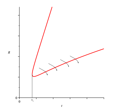
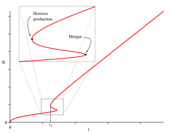
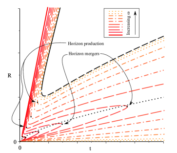
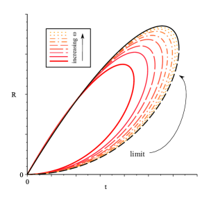
where is the areal radius of spacetime. In general, this equation can only be solved numerically or, if its solutions can be expressed in analytical form, they are usually implicit. A rather common phenomenon encountered in the study of dynamical AHs lastbook is the sudden appearance of a pair of AHs, or the merging and disappearance of pairs of AHs HusainMartinezNunez . The two common phenomenologies are illustrated in Figs. 1 and 2.
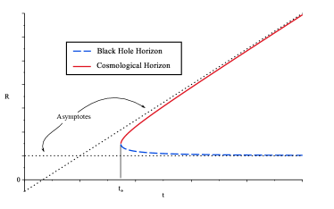
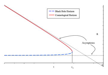
In Fig. 1, a naked singularity present in an inhomogeneous universe gets covered by a black hole AH which appears together with a cosmological AH at a critical time : the black hole AH starts shrinking while the cosmological AH expands. This type of phenomenology is encountered in the McVittie solution Nolan ; AndresRoshina ; KaloperKlebanMartin10 ; LakeAbdelqader11 ; SilvaFontaniniGuariento12 and is interpreted in AndresRoshina . Following the widely known example of the Schwarzschild-de Sitter-Kottler spacetime (which is a special case of McVittie for a static de Sitter ‘background’), for times less than the critical instant the black hole AH is larger than the cosmological AH and cannot be seen; at the critical time the two AHs coincide (and they are instantaneously null), or they are ‘created’; while for the black hole AH fits into the cosmological AH. The reversal of this, shown in Fig. 2, where the expansion is accelerating from an initially quasi-static state, the cosmological horizon shrinks and eventually engulfs the black hole horizon, leaving a naked singularity.
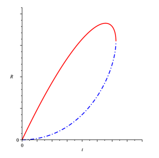
The picture corresponding to Fig. 1 for the actual exact McVittie solution at later times is richer than this simple scenario. In that case the black hole AH keeps shrinking and asymptotes to a spacelike spacetime singularity located at a finite areal radius. This singularity divides spacetime into two disconnected regions (but these two spacetime regions don’t communicate—for all purposes they describe two different spacetimes). In the charged version of McVittie spacetime, formally, a third root exists in the spacetime region below the spacelike singularity. Depending on the region of parameter space, this third root either asymptotes to a finite radius inside the spacelike singularity as shown in Fig. 3
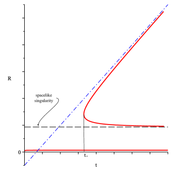
or approaches this singularity from below, as shown in Fig. 4.
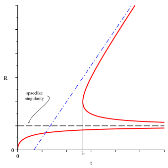
The asymptotic structure of the innermost pair of horizons in this charged case matches what one would expect from knowledge of the Reissner Nordstrom charged static black hole which possesses an inner and outer event horizon the locations of which coincide with the asymptotes of their counterparts in charged McVittie (including in the critical Reissner Nordstrom case). After the Einstein-Straus Swiss-cheese model EinsteinStraus , the McVittie solution of GR is probably the most famous spacetime describing a local object embedded in a universe and this is likely the first phenomenology of AHs that one is bound to encounter in a survey of the literature Galaxies ; lastbook .
It should be pointed out that the McVittie and charged McVittie solutions are special in that they have zero radial flux of matter at the black hole horizon. Allowing for a radial energy flux into the central singularity, one is led to the so-called generalized McVittie solutions. The generalized McVittie line element is given by AudreyPRD
| (2) | |||||
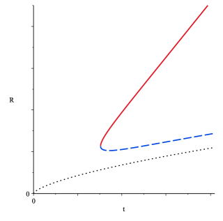
with an arbitrary function of time and (where is the Einstein tensor), corresponding to a radial energy flow. The generalized McVittie spacetime has a singularity at (corresponding to in the notations of AudreyPRD ), where the energy density and the pressure diverge AudreyPRD . The AH structure, as generically shown in Fig. 5, is similar to the McVittie case but with an expanding black hole horizon as the black hole accretes energy and becomes more massive (see SilvaGuarientoMolina15 ). However, when the surrounding matter is of phantom type, the black hole can lose mass and the black hole horizon can shrink, as discussed in GaoChenFaraoniShen08 .
The phenomenology of AHs reported in Figs. 1, 3, 4, and 5 will be referred to as fold-type or ‘C-curve’ behaviour due to the shape of the curve. This phenomenology is reported also for Lemaître-Tolman-Bondi spacetimes BoothBritsGonzalezVDB ; GaoChenShenFaraoni11 .
I.2 Cusp-type or ‘S-curve’ horizons
A second type of phenomenological behaviour of AHs of cosmological black holes is the one represented generally in Fig. 6, which we will refer to as cusp-type or ‘S-curve’.
This terminology comes from catastrophe theory where curves of this shape describe what are called cusp-type catastophies. In this case, a single AH exists from the initial Big Bang, then two initially coincident AHs appear at time . The larger (cosmological) AH expands forever, while the smaller (black hole) one shrinks, eventually meeting the smallest AH which in the meantime has been expanding. When these two black hole AHs (interpreted as inner and outer black hole AHs HusainMartinezNunez ) meet, they ‘annihilate’ and disappear, leaving behind a naked central singularity in a cosmological ‘background’. This S-curve behaviour was discovered by Husain, Martinez, and Nuñez in their scalar field solution HusainMartinezNunez and was subsequently reported myClifton in the Clifton solution of metric gravity CliftonCQG2006 and in the Clifton-Mota-Barrow family of solutions of Brans-Dicke theory CliftonMotaBarrow in a certain region of the parameter space climobarr . Indeed, Fig. 6 is precisely the AH structure for the Husain, Martinez, and Nuñez solution (with their parameter HusainMartinezNunez ). In Fig. 7 we also show the cusp-type behaviour of the AHs for an exact CMB solution which we will discuss more fully in the following section.

Thus far, the s-curve and the c-curve phenomenologies of AHs seem completely disconnected and mutually exclusive—and what could the s-curve behaviour with three AHs have in common with spacetimes containing only two AHs and a singularity at a finite radius? Here we will show that these two phenomenologies are not disconnected and that C-curve spacetimes correspond indeed to a limit of S-curve spacetimes when the lower bend in the S (where two AHs annihilate) is pushed to infinity. In this limit a spacetime singularity appears at a finite radius, precisely at the location that would be occupied by the would-be critical AH resulting from the instantaneous merging of the inner and outer black hole AHs. This insight comes from the limit to GR of the Clifton-Mota-Barrow family of Brans-Dicke solutions.
II The Clifton-Mota-Barrow family of spacetimes
The Clifton-Mota-Barrow family (CMB) of solutions of Brans-Dicke theory is written as CliftonMotaBarrow
| (3) |
in isotropic coordinates, where
| (4) | |||||
| (5) | |||||
| (6) | |||||
| (7) | |||||
| (8) |
and the Brans-Dicke scalar field is given by CliftonMotaBarrow
| (9) |
Here is the Brans-Dicke parameter, is a mass parameter, , and are positive constants (, , and are not independent). The matter source is a perfect fluid with energy density , pressure , and equation of state , where is a constant CliftonMotaBarrow .
The structure of the apparent horizons depends crucially on the equation of state parameter and the Brans-Dicke parameter . For completeness, when the expansion is positive, the condition (1) reduces for this metric to
| (10) |
where is the areal radius. This condtion can have 0, 1, 2 or 3 roots for positive with the generic behaviour being that which is shown in Fig. 7 or alternatively a bubble like configuration as shown in Fig. 8, which is a variant on the basic horizon merger structure which we described in Fig. 2.
II.1 The limit of the Clifton-Mota-Barrow family of spacetimes
The Clifton-Mota-Barrow family of spacetimes was interpreted in Ref. climobarr , in which the limit to GR was briefly discussed, although the connection between S-curve and C-curve was missed there because of an incorrect figure (Fig. 4 of climobarr ).
The limit of the line element (3) is quite interesting in itself: it is a late-time attractor of the generalized McVittie class of solutions (2) of the Einstein equations. We have already remarked that there is no uniqueness theorem analogous to the Israel-Carter-Robinson theorems for non-isolated and/or dynamical black holes in GR. However, within the restricted class of generalized McVittie solutions (2) AudreyPRD ; GaoChenFaraoniShen08 ; GuarientoAfshordi1 ; GuarientoAfshordi2 , there is a unique late-time attractor FaraoniGaoChenShen09 and this is the only known such occurrence among classes of spacetimes describing cosmological black holes.
The limit of the line element is
| (11) | |||||
| (12) | |||||
| (13) |
which is recognized as a special case of a generalized McVittie metric (2). The special case , where is a constant, is the late-time attractor of this class FaraoniGaoChenShen09 and is the limit of the Clifton-Mota-Barrow spacetime (3)-(8). The singularity of this attractor spacetime is located at the areal radius and it expands comoving with the cosmic substratum.
The limit of the Clifton-Mota-Barrow spacetime has a peculiar feature: its two AHs are given by the simple expressions FaraoniGaoChenShen09
| (14) |
where the subscripts C and BH stand for cosmological and black hole AHs, respectively, and an overdot denotes differentiation with respect to the comoving time . It is very rare to be able to locate AHs analytically, and even rarer to do so explicitly lastbook . Eq. (14) states that there are two and only two AHs provided that
| (15) |
where , in the limit, and , otherwise there are none.
The case we will be interested in mainly is a dust-dominated universe which is described by the range . In this case the exponent is negative which corresponds to the equation of state parameter and hence the universe is decelerated in this case. This will be the main case we are interested in because it is the case in which our equivalence between S- and C-curve horizons is most transparent.
In this case the two distinct AHs are present for
| (16) |
These two AHs are created at and subsequently have a C-curve behaviour as shown in Fig. 9. This is exactly as we showed schematically in Fig. 5 as an example of an accreting cosmological black hole. In addition to the two apparent horizons there is a new finite-radius singularity indicated in Fig. 9 by the black dotted line.
Let us follow the evolution of the AHs of the Clifton-Mota-Barrow spacetime as the Brans-Dicke parameter becomes larger and larger. This is limit is shown in the various S-curves333Fig. 4 of Ref. climobarr incorrectly depicts them as C-curves instead. of Fig. 10 for increasing values of :
as grows, these curves become more and more stretched and their lower bend (where the two innermost AHs merge and disappear) occurs at times which are larger and larger. As , also and the S-curve is broken, becoming a C-curve and the lowest branch of the S converges to 0 for all . A spacetime singularity appears in this limit at a finite areal radius, which is the location of the would-be ‘critical’ horizon resulting from the merger of the inner and outer black hole AHs occurring for finite values of .
The inner horizon (the limit of the lower leg of the S-curve) is usually not reported in the literature in plots describing the AHs structure of McVittie and generalized McVittie solutions because it belongs to a different spacetime disconnected from the previous one by the finite radius singularity. However, plotting the three AHs together clearly shows how the S-curve breaks into a C-curve in the limit. It looks as if AHs ‘want’ to disappear in pairs and, by making only one of them survive in the limit, one somehow ‘splits’ the spacetime instead. The mechanism and the deep reasons for this process are completely unclear, but one cannot help feeling that the structure of these AHs is telling us something about the spacetime itself.
While the AHs momentarily coinciding at the lower bend of the S-curve are instantaneously null (with there), the black hole AH asymptoting to the finite-radius singularity in the generalized McVittie metric quickly becomes spacelike (with ). The AH in the disconnected spacetime “below” the finite radius singularity also becomes spacelike with .
II.2 Other parameter ranges: and
When (equivalent to and corresponding to an accelerated universe) the exponent is positive, the inequality (15) is satisfied, and there are two AHs for times less than a critical time
| (17) |
The two AHs exist during all times approaching each other, then coincide and disappear at the time , as we generically showed in Fig. 8.
One can interpret this behaviour as a black hole which is ‘swallowed’ by the cosmological horizon as the latter shrinks due to the increasing acceleration of the expansion while for former grows as matter is accreted across it.444Due to a peculiarity of the power law, in fact accelerating spacetimes have a small for early times and hence the cosmological horizon in that case always sits outside the black hole horizon, all the way back to . On the other hand, decelerating spacetimes have a which in fact diverges for small , which is the reason why decelerated spacetimes begin their lives with a cosmological horizon which is much smaller than the black hole horizon. Effectively, decelerated spacetimes start off expanding very rapidly while accelerated spacetimes start off expanding mildly.
Again we can follow the apparent horizon structure in the full CMB solution as the limit is carried out. In Fig. 11 we choose and plot the horizons over time for increasing values of . The AHs form a closed curve touching the origin for each value of so the limit is less interesting and does not interpolate between cusp and fold structures.
This accelerated expansion AHs are interpreted as a special case of the fold-type, with the fold pushed all the way back to the big bang singularity.
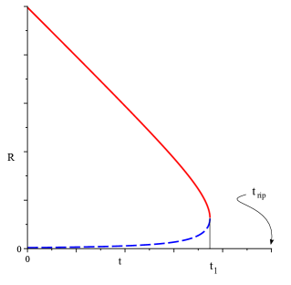
For completeness we mention the spacetimes (corresponding to and to a phantom universe with a big rip singularity at the time ). The exponent is again negative and the scale factor is
| (18) |
the inequality (15) is satisfied, and there are two AHs, for times
| (19) |
The two AHs coincide and disappear at as shown in Fig. 12. Note that, in our universe, phantom energy would not have dominated forever but would have started dominating only recently and the behaviour described by the formal solution (18) and shown for illustration would have to be changed accordingly.
III Conclusions
Dynamical and non-asymptotically flat black holes are best characterized by their AHs. The known exact solutions of the Einstein equations which are spherically symmetric and represent dynamical black holes embedded in FLRW spaces exhibit two types of phenomenological behaviours, here dubbed “S-curve” and “C-curve” types because of the shape of the AH radii versus comoving time. These phenomenologies show up also in (rare) cosmological black hole solutions of scalar-tensor and gravity. Thus far, these two types of AHs behaviours appeared to be completely disconnected. However, by taking the limit to GR of the Clifton-Mota-Barrow spacetimes, one understands that the C-curve is just a limit of the S-curve as the lower bend of the S approaches infinity. Because no spacetime is known in which the AHs exhibit S-curve behaviour and can be located analytically and explicitly, one cannot control directly the location of this lower bend and adjust a parameter in order to push this bend to infinity. However, the limit of the Clifton-Mota-Barrow class of solutions of Brans-Dicke theory does exactly that for us: the C-curve is obtained essentially as the limit of S-curves as the lower bend of the S is pushed to infinity. Therefore, this limit to GR connects what thus far appeared to be two completely disconnected phenomenologies of AHs. What is more, AHs usually appear or disappear in pairs HusainMartinezNunez ; Nolan ; AndresRoshina and inner/outer black hole AHs, in particular, seem to want to do the same: if only one horizon is selected through the limit to GR, a spacetime singularity appears and the other AH is relegated to the associated (but disconnected) spacetime “below the singularity”. The reason why pairs of AHs can only be split by introducing a spacetime singularity between them remains a mystery.
Acknowledgements.
This research is supported by Bishop’s University and by the Natural Sciences and Engineering Research Council of Canada (NSERC).References
- (1) J. Thornburg, Living Rev. Relat. 10, 3 (2007); T.W. Baumgarte, S.L. Shapiro, Phys. Rept. 376, 41 (2003); T. Chu, H.P. Pfeiffer, M.I. Cohen, Phys. Rev. D 83, 104018 (2011).
- (2) G.W. Gibbons and S.W. Hawking, Phys. Rev. D 15, 2738 (1977).
- (3) R.M. Wald and V. Iyer, Phys. Rev. D 44, R3719 (1991); E. Schnetter and B. Krishnan, Phys. Rev. D 73, 021502 (2006).
- (4) V. Faraoni, Galaxies 1, 114 (2013).
- (5) V. Faraoni, Cosmological and Black Hole Apparent Horizons (Springer, New York), forthcoming 2015.
- (6) A.B. Nielsen and M. Visser, Class. Quantum Grav. 23, 4637 (2006).
- (7) G.C. McVittie, Mon. Not. R. Astr. Soc. 93, 325 (1933).
- (8) A. Krasiński, Inhomogeneous Cosmological Models (Cambridge University Press, Cambridge, 1997).
- (9) M. Carrera and D. Giulini, Rev. Mod. Phys. 82, 169 (2010).
- (10) B.C. Nolan, Class. Quantum Grav. 16, 1227 (1999); Class. Quantum Grav. 16, 3183 (1999); Phys. Rev. D 58, 064006 (1998).
- (11) V. Faraoni, A.F. Zambrano Moreno, and R. Nandra, Phys. Rev. D 85, 083526 (2012).
- (12) N. Kaloper, M. Kleban, and D. Martin, Phys. Rev. D 81, 104044 (2010).
- (13) K. Lake and M. Abdelqader, Phys. Rev. D 84, 044045 (2011).
- (14) R. Nandra, A.N. Lasenby, and M.P. Hobson, Mon. Not. R. Astr. Soc. 422, 2931 (2012).
- (15) R. Nandra, A.N. Lasenby, and M.P. Hobson, Mon. Not. R. Astr. Soc. 422, 2945 (2012).
- (16) A. da Silva, M. Fontanini, and D.C. Guariento, Phys. Rev. D 87, 064030 (2013).
- (17) Y.P. Shah and P.C. Vaidya, Tensor 19, 191 (1968).
- (18) C.J. Gao and S.N. Zhang, Phys. Lett. B 595, 28 (2004).
- (19) V. Faraoni, A.F. Zambrano Moreno, and A. Prain, Phys. Rev. D 89, 103514 (2013).
- (20) V. Faraoni and A. Jacques, Phys. Rev. D 76, 063510 (2007).
- (21) E. Abdalla, N. Afshordi, M. Fontanini, D.C. Guariento, and E. Papantonopoulos, Phys. Rev. D 89, 104018 (2014).
- (22) N. Afshordi, M. Fontanini, and D.C. Guariento, Phys. Rev. D 90, 084012 (2014).
- (23) V. Husain, E.A. Martinez, and D. Nuñez, Phys. Rev. D 50, 3783 (1994).
- (24) O.A. Fonarev, Class. Quantum Grav. 12, 1739 (1995).
- (25) H. Maeda, arXiv:0704.2731.
- (26) I. Booth, L. Brits, J.A. Gonzalez, and V. Van den Broeck, Class. Quantum Grav. 23, 413 (2006).
- (27) C. Gao, X. Chen, Y.-G. Shen, and V. Faraoni, Phys. Rev. D 84, 104047 (2011).
- (28) J. Sultana and C.C. Dyer, J. Math. Phys. 45, 4764 (2004).
- (29) H. Saida, T. Harada, and H. Maeda, Class. Quantum Grav. 24, 4711 (2007).
- (30) V. Faraoni, Phys. Rev. D 76, 104042 (2007).
- (31) B.R. Majhi, J. Cosmol. Astropart. Phys. 1405, 014 (2014); Phys. Rev. D 90, 044020 (2014).
- (32) M.L. McClure and C.C. Dyer, Class. Quantum Grav. 23, 1971 (2006); Gen. Rel. Gravit. 38, 1347 (2006); M.L. McClure, K. Anderson, and K. Bardahl, arXiv:0709.3288; Phys. Rev. D 77, 104008 (2008); M.L. McClure, Cosmological Black Holes as Models of Cosmological Inhomogeneities, PhD thesis, University of Toronto, 2006.
- (33) J. Lindesay, Found. Phys. 37, 1181 (2007); J. Lindesay, Foundations of Quantum Gravity (Cambridge University Press, Cambridge, 2013), p.282; J. Lindesay and P. Sheldon, Class. Quantum Grav. 27, 215015 (2010).
- (34) T. Clifton, D.F. Mota, and J.D. Barrow, Mon. Not. R. Astr. Soc. 358, 601 (2005).
- (35) V. Faraoni, V. Vitagliano, T.P. Sotiriou, and S. Liberati, Phys. Rev. D 86, 064040 (2012).
- (36) V. Faraoni and A.F. Zambrano Moreno, Phys. Rev. D 86, 084044 (2012).
- (37) T. Clifton, Class. Quantum Grav. 23, 7445 (2006).
- (38) V. Faraoni, Class. Quantum Grav. 26, 195013 (2009); V. Faraoni, in Proceedings of Cosmology, Quantum Vacuum, and Zeta Functions, Springer Proceedings in Physics vol. 137, Barcelona 2010, S.D. Odintsov, D. Saez-Gomez, and S. Xambo-Descamps eds. (Springer, New York, 2011), 173.
- (39) A. Einstein and E.G. Straus, Rev. Mod. Phys. 17, 120 (1945); Rev. Mod. Phys. 18, 148 (1946).
- (40) C. Gao, X. Chen, V. Faraoni, and Y.-G. Shen, Phys. Rev. D 78, 024008 (2008).
- (41) A. da Silva, D.C. Guariento, and C. Molina, Phys. Rev. D 91, 084043 (2015).
- (42) V. Faraoni. C. Gao, X. Chen, and Y.-G. Shen, Phys. Lett. B 671, 7 (2009).