Maps for global separation of roots

Abstract

Two simple predicates are adopted and certain real-valued piecewise continuous functions are constructed from them. This type of maps will be called quasi-step maps and aim to separate the fixed points of an iteration map in an interval. The main properties of these maps are studied. Several worked examples are given where appropriate quasi-step maps for Newton and Halley iteration maps illustrate the main features of quasi-step maps as tools for global separation of roots.

Key words: Step function; Fixed point; Iteration map; Newton map; Halley map; Sieve of Eratosthenes.

2010 Mathematics Subject Classification: 65-05, 65H05, 65H20, 65S05.

1 Introduction

Separation of real roots is a classical subject dating back to the seminal work of Lagrange [11] on polynomial equations. In this paper we aim to offer other computational perspective to the global separation of roots of a general nonlinear equation by constructing certain iteration maps which will be called quasi-step maps.

We consider the problem of finding the roots of a given real-valued equation $f(x)=0$ on a closed interval $D=[a,b]$, which we write as a fixed point equation $x=g(x)$. Let ${\cal Z}=\{z_{1},z_{2},\ldots,z_{n}\}$ be the non-empty set of (distinct) fixed points of the map $g$. If the set ${\cal Z}$ was known, a good model of a map separating the fixed points of $g$ in the interval $D$ is the following step map $\Psi$:

$$\Psi(x)=\sum_{i=1}^{n}z_{i}{\cal X}_{I_{i}}(x),\quad x\in D,$$ (1)

where ${\cal X}_{I_{i}}$ is the characteristic function of the subinterval $I_{i}\subset D$ (i.e. ${\cal X}_{I_{i}}(x)=1$ for $x\in I_{i}$ and ${\cal X}_{I_{i}}(x)=0$ otherwise) and the intervals $I_{i}$ are pairwise disjoint.

In general, a step map of the form (1) is not directly feasible from $g$ since the set of fixed points ${\cal Z}$ is unknown. It is then natural to look for a map $\widetilde{\Psi}$ of the form

$$\widetilde{\Psi}(x)=\sum_{i=1}^{s}\widetilde{g}(x){\cal X}_{J_{i}}(x),\qquad\text{$x\in D$}$$ (2)

where:

(a) The union of the intervals $J_{i}$ is contained in $D$ and each $J_{i}$ contains at least a fixed point of $g$.

(b) The function $\widetilde{g}$ is continuous on each subinterval $J_{i}$;

(c) The function $\widetilde{g}$ preserves the fixed points of $g$ on each $J_{i}$.

Like the map (1), the map (2) may be seen as a tool for separation of points in ${\cal Z}$. A map $\widetilde{\Psi}$ of the type (2) will be called a quasi-step map (see Definition 2.1).

The construction of a map $\widetilde{g}$ as in (2) will be done by considering one or more predicates which are based upon the map $g$ and the domain $D$. The predicates to be used hereafter are denoted by $\mathbb{P}_{0}$ and $\mathbb{P}_{1}$. Given a constant $d>0$, these predicates are:

$$\begin{array}[]{ll}\mathbb{P}_{0}:&x\in D,\,\,\text{ $y=g(x)\in D$ and $|y-x|<d$},\\ \mathbb{P}_{1}:&\text{$x\in D$, $y=g(x)\in D$, $w=g(y)\in D$ and $|w-y|\leq|y-x|$}.\end{array}$$

For any point $x\in D$ the predicate $\mathbb{P}_{0}$ tests the image $y=g(x)$ while $\mathbb{P}_{1}$ tests two applications of $g$.

A collection of subintervals $J_{i}\subset D$ is induced by a sort of divide and conquer effect from the action of one or both predicates. Moreover when we use the predicate $\mathbb{P}_{0}$ (resp. $\mathbb{P}_{1}$) the value assigned to $\widetilde{g}(x)$ in (2) will be $y=g(x)$ (resp. $w=g(g(x)))$ for all points $x\in D$ for which $\mathbb{P}_{0}$ (resp. $\mathbb{P}_{1}$) is true. All the other points $x\in D$ for which the predicate under consideration is false, the value zero will be assigned to $\widetilde{g}$. A map $\widetilde{\Psi}$ as in (2) constructed from one or more predicates will be called an ‘educated’ map in the sense that the construction of this map is based on the action of the predicate(s).

As explained in detail in Section 2, under mild assumptions on $g$, the above predicates $\mathbb{P}_{0}$ and $\mathbb{P}_{1}$ lead to quasi-step maps of type (2), separating fixed points of the initial map $g$. As we will see, it is convenient to choose an initial map $g$ satisfying the property of attracting points in $D$ which are sufficiently close to the fixed points. Fortunately such a choice of maps $g$ does not presents any difficulty due to the plethora of iteration maps in the literature enjoying the referred attracting property. Among them we will consider the celebrated Newton-Raphson and Halley maps since as it is well known, under mild assumptions, both maps have at least linear local convergence and so guaranteeing the referred attracting property ([20], [5], [9],[16], [25], [21], and [14]). The proofs of how the predicates will lead to quasi-step maps separating fixed points of $g$, given in Section 2, use mainly the fixed point theorem for closed and bounded real intervals or the contraction Banach principle (see for instance [16], [17], [26]).

The paper is divided in two parts. In the first part (Section 2) the main theoretical results are established and the second part deals with worked examples (Section 3). In Section 2 we show under which conditions on $g$, or on its fixed points, the predicates $\mathbb{P}_{0}$ and $\mathbb{P}_{1}$ will enable the construction of quasi-step maps providing a global separation of the fixed points of $g$ (propositions 1 and 2). A brief reference on how the composition of quasi-step maps may be implemented to achieve accurate approximations of fixed points of $g$ is also made (see paragraph 2.1).

Section 3 is devoted to examples illustrating the separation of fixed points by constructing quasi-step maps from the predicates $\mathbb{P}_{0}$ and $\mathbb{P}_{1}$. We begin with a family of trigonometrical functions $f_{k}$ presented by Charles Pruitt in [19]. Due to the fact that Pruitt functions only admit integer zeros (cf. Proposition 3) we are able to numerically construct (Example 1) a step map which provides not only all the zeros of $f_{3}$ but it also enables to distinguish composite numbers from prime numbers in the interval of definition of the map. Pruitt functions are also used (Examples 2 and 3) to illustrate the main features of several quasi-step maps derived from Newton and Halley maps educated by the predicates $\mathbb{P}_{0}$ and $\mathbb{P}_{1}$. In Example 4 a strongly oscillating transcendental function $f$ is considered. Certain discretized versions of composed Halley educated maps are applied in order to globally separate a great number of zeros of $f$ producing at the same time accurate values for them.

2 Separation of fixed points

In this section we show how the predicates $\mathbb{P}_{0}$ and $\mathbb{P}_{1}$ will enable the construction of quasi-step maps of type (2) from a given function $g$. Given an interval $D=[a,b]$ and a constant $d>0$, the predicates to be considered are the following:

$$\mathbb{P}_{0}: \;\;x\in D,\,\,\text{ $y=g(x)\in D$ and $|y-x|<d$},$$ (3)

$$\mathbb{P}_{1}: \;\;\text{$x\in D$, $y=g(x)\in D$, $w=g(y)\in D$ and $|w-y|\leq|y-x|$}.$$ (4)

Note that if $x$ is a fixed point of $g$, the predicates $\mathbb{P}_{0}$ and $\mathbb{P}_{1}$ hold true for $x$. Moreover, assuming that $g$ is continuous near each fixed point, there are subintervals $J_{i}$ of $D$, containing fixed points of $g$, where the predicates hold true as well. We now precise the notion of a quasi-step map.

Definition 2.1.

Let $g:\mathbb{R}\rightarrow\mathbb{R}$ be a function and $D=[a,b]\subset\mathbb{R}$. A quasi-step map associate to $g$ is a function $\widetilde{\Psi}$ of the form

$$\widetilde{\Psi}(x)=\sum_{k=1}^{s}\widetilde{g}(x)\,{\cal X}_{J_{k}}(x),\quad\text{if $x\in D$}$$ (5)

where

• Any subinterval $J_{k}$ contains at least one fixed point of $g$ and the union of these intervals is contained in $D$ (i.e. $J=\cup_{k=1}^{s}J_{k}\subseteq D$);

• The function $\widetilde{g}$ is continuous on each subinterval $J_{k}$;

• $\widetilde{g}(z)=z$ for any fixed point $z$ of $g$ belonging to $J_{k}$.

We note that if in the above definition all the subintervals $J_{i}$ are pairwise disjoint and the number $s$ coincides with the number $n$ of the fixed points of $g$, the quasi-step map $\widetilde{\Psi}$ separates all the fixed points of $g$ in $D$.

For practical purposes we chose either one or both predicates $\mathbb{P}_{0}$, $\mathbb{P}_{1}$ to construct a quasi-step map as in (5). Such a map will be called ‘educated’  by the predicate(s) in the sense that the map results from the action of the predicate(s) on the interval $D$.

Definition 2.2.

(Educated map)

Let $g$ be a real-valued map and consider the interval $D\subseteq\mathbb{R}$, ${\cal X}_{B}$ the characteristic function of a set $B$, $d$ a positive constant, and $\mathbb{P}_{0}$, $\mathbb{P}_{1}$ the predicates in (3) and (4), respectively. Let $\{L_{k}^{i}\}$ be the collection of subintervals of $D$ where the predicate $\mathbb{P}_{i}$ ($i=0,1$) holds true.

• The quasi-step map

  $$\widetilde{\Psi}_{i}(x)=\sum_{k}{\widetilde{g}}_{i}(x)\,{\cal X}_{L^{i}_{k}}(x),\quad x\in D$$

  is said to be educated by the predicate $\mathbb{P}_{i}$, if ${\widetilde{g}}_{i}(x)=0$ for all $x\in D\setminus\cup_{k}L_{k}^{i}$, and on each $L_{k}^{i}$: ${\widetilde{g}}_{i}=g$ for $i=0$ and ${\widetilde{g}}_{i}=g\circ g$ for $i=1$.

• The quasi-step map

  $$\widetilde{\Psi}(x)=\sum_{k}{\widetilde{g}}(x)\,{\cal X}_{J_{k}}(x),\quad x\in D$$

  is said to be educated by both predicates $\mathbb{P}_{0}$ and $\mathbb{P}_{1}$, if ${\widetilde{g}}_{i}(x)=0$ for $x\in D\setminus\cup_{k}(L^{0}_{k}\cap L^{1}_{k})$ and ${\widetilde{g}}=g\circ g$ in each $J_{k}=L^{0}_{k}\cap L^{1}_{k}$.

Note that a map educated by the predicate $\mathbb{P}_{0}$ is a map which is necessarely zero at all the $x\in D$ such that $(x,g(x))$ does not lie in a band of width $2d$ centered at the line $y=x$. This is the reason why we will call $d$ the vertical displacement parameter. On the other hand, the predicate $\mathbb{P}_{1}$ tests $y=g(x)\in D$ and $w=g(y)\in D$ satisfying $|w-y|\leq|y-x|$. Since, for $y\neq w$ the quantity $(w-y)/(y-x)$ represents the slope of the line through the points $(x,y)$ and $(y,w)$ we call $\mathbb{P}_{1}$ the slope predicate.

We note that the ‘education’  of a map is an a priori global technique (i.e. no initial guesses are required) which may be seen as a counterpart of the classical a posteriori stopping criteria used in root solvers algorithms for local search of roots (see for instance [15] and references therein).

Although in this work we only adopt the predicates $\mathbb{P}_{0}$ and $\mathbb{P}_{1}$, other predicates could be considered in order that the respective educated map will satisfy other criteria such as monotony or alternate local convergence. Also, an ‘education’  of the map $f$ instead of the map $g$ may be of interest, namely in the light of well known sufficient conditions for local monotone convergence of Newton and Halley methods (see for instance [4], [13]).

2.1 Quasi-step maps from the predicates $\mathbb{P}_{0}$ and $\mathbb{P}_{1}$

In this paragraph we address the question of knowing what kind of functions $g$ may be chosen in order to construct educated maps from the predicates $\mathbb{P}_{0}$ and $\mathbb{P}_{1}$ leading to a global separation of fixed points of $g$. In particular, with respect to the predicate $\mathbb{P}_{0}$ we will show that the contractivity of $g$ near each of its fixed points and a conveniently chosen vertical displacement parameter $d$, provide quasi-step maps isolating fixed points of $g$ in $D$. In the case of the predicate $\mathbb{P}_{1}$, under mild hypotheses on $g$, this predicate implies the contractivity of $g$ near fixed points and consequently enabling the construction of an educated map by $\mathbb{P}_{1}$ isolating fixed points of $g$ as well.

In what follows we assume that a real-valued map $g$ is given, $D$ is the closed interval $D=[a,b]\subset\mathbb{R}$, and ${\cal X}_{B}$ denotes the characteristic function of the set $B$. We denote by ${\cal Z}\subset D$ the (non-empty) finite set of the fixed points of $g$, say $z_{1},z_{2},\ldots,z_{n}$.

Lemma 1.

Let $d$ be a positive number and $z$ a fixed point of $g$ belonging to $D=[a,b]$. If $g$ is contractive in the interval

$$I_{z}=[z-d,z+d]\subseteq D,$$

and the predicate $\mathbb{P}_{0}$ holds true for any point of $I_{z}$, then there exists a bounded closed interval

$$J_{z}=[z-\epsilon,z+\epsilon]\subseteq I_{z},\quad\epsilon>0$$

such that the map

$$\widetilde{\Psi}_{z}(x)=\widetilde{g}_{z}(x)\,{\cal X}_{J_{z}}(x)\;\;x\in D,$$

with $\widetilde{g}_{z}(x)=0$ if $x\in D\setminus J_{z}$ and $\widetilde{g}_{z}=g$ in $J_{z}$, isolates the (unique) fixed point $z$ of $g$ in $D$.

Proof.

First note that the hypothesis on the predicate $\mathbb{P}_{0}$ gives

$$\begin{array}[]{l}|g(x)-x|<d,\quad x\in I_{z}.\end{array}$$ (6)

The points $(x,g(x))$ of the plane satisfying the above inequality (6) belong to a closed planar region delimited by the parallel horizontal lines $y=z+d$, $y=z-d$ and the oblique parallel lines $y=x+d$, $y=x-d$. Denote by ${\cal P}$ the parallelogram bounding such region and note that the diagonals of ${\cal P}$ intersect at the point $A=(z,z)$.

Let ${\cal D}$ be the closed disk of radius $r=d/\sqrt{2}$ centered at $A$. This disk is inscribed in the region delimited by ${\cal P}$. As by hypothesis $g$ is contractive in $I_{z}$, then $g$ is continuous in this interval. So, there exists $\delta>0$ such that

$$x\in[z-\delta,z+\delta]\Longrightarrow|g(x)-z|<r.$$

Also by the contractivity of $g$, there exists a number $K$, with $0\leq K<1$, ($K$ is a contractivity constant) such that the graph of $g$ lies inside a cone section with vertex at $A$ and whose edges make an angle $|\alpha|=\arctan(K)<\pi/4$ at the vertex $A$. Therefore, there exists a number $0<\epsilon<r$ such that the square region ${\cal S}=[z-\epsilon]\times[z+\epsilon]\subset\mathbb{R}^{2}$ is contained in the disk ${\cal D}$. Moreover, for the closed interval $J_{z}=[z-\epsilon,z+\epsilon]$ we have $g(J_{z})\subseteq J_{z}$. As $J_{z}$ is closed and $g$ is contractive in $J_{z}$, it follows from the Banach contraction principle that there is a unique fixed point of $g$ in $J_{z}$, which is obviously the point $z$. It is now immediate that the map $\widetilde{\Psi}_{z}$ isolates $z$ in $D$. ∎

We now assume that the set ${\cal Z}$ of the fixed points of $g$ is ordered, and define the resolution $\eta$ of ${\cal Z}$ as the minimum of the distances between any pair of consecutive points of ${\cal Z}$.

Proposition 1.

Let ${\cal Z}=\{z_{1},\ldots,z_{n}\}$ be the set of the fixed points of $g$ and $\eta$ its resolution. Consider $g$ and $\mathbb{P}_{0}$ satisfying the conditions of Lemma 1 on each interval $I_{z_{i}}=[z_{i}-d,z_{i}+d]$ with

$$d<\frac{\eta}{2}.$$

Then, there exists a collection of disjoint subintervals $J_{z_{i}}\subset I_{z_{i}}$ with $J=\cup_{i=1}^{n}J_{z_{i}}\subset D$, and maps $\widetilde{g}_{z_{i}}$ defined as $\widetilde{g}_{z_{i}}(x)=0$, if $x\in D\setminus J$ and $\widetilde{g}_{z_{i}}=g$ in each interval $J_{z_{i}}$, such that

$$\widetilde{\Psi}(x)=\sum_{i=1}^{n}\widetilde{g}_{z_{i}}(x)\,{\cal X}_{J_{z_{i}}}(x),\quad\text{$x\in D$}$$

is an educated map by $\mathbb{P}_{0}$, separating all the fixed points of $g$ in $D$.

Proof.

The hypotheses on $g$ and $\mathbb{P}_{0}$ implies that Lemma 1 is satisfied for each fixed point $z_{i}$. That is: (i) there exists a closed subinterval $J_{z_{i}}=[z_{i}-\epsilon_{i},z_{i}+\epsilon_{i}]$ of $I_{z_{i}}=[z_{i}-d,z_{i}+d]\subset D$; (ii) the map $g$ is continuous in $J_{z_{i}}$; (iii) the fixed point $z_{i}$ is the unique fixed point of $g$ in $J_{z_{i}}$.

Hence, as $d<\eta/2$ the subintervals $J_{z_{i}}$ are obviously disjoint and, by the definition of an educated map by $\mathbb{P}_{0}$ (cf. Definition 2.1), the map $\widetilde{\Psi}$ is an educated map separating the fixed points of $g$. ∎

We now explain the role of the slope predicate $\mathbb{P}_{1}$ in the construction of a quasi-step map. Let us begin with a lemma showing that for a given fixed point $z$ verifying $g^{\prime}(z)\neq 1$ (i.e. a non-neutral fixed point), if the predicate $\mathbb{P}_{1}$ holds in a certain interval containing $z$ it is possible to isolate this fixed point.

Lemma 2.

Let $z\in D$ be a fixed point of a map $g$ which is of class $C^{1}$ in the interval $X_{z}=[z-\epsilon,z+\epsilon]\subset D$ ($\epsilon>0$). Assume that $g^{\prime}(z)\neq 1$ and $\mathbb{P}_{1}$ holds true for all non-fixed points of $g$ belonging to $X_{z}$. Then,

• There is a closed bounded subinterval $\widetilde{X}_{z}=[z-\mu,z+\mu]$ of $X_{z}$ where the map $g$ is contractive.

• The map

  $${\widetilde{\Psi}}_{z}(x)=\widetilde{g}_{z}(x)\,{\cal X}_{\widetilde{X}_{z}}(x),\quad\text{$x\in D$},$$ (7)

  with $\widetilde{g}_{z}(x)=0$ if $x\in D\setminus\widetilde{X}_{z}$ and $\widetilde{g}_{z}=g\circ g$ in $\widetilde{X}_{z}$, isolates the fixed point $z$.

Proof.

(i) Note that the inequality in $\mathbb{P}_{1}$ means that $|g(g(x)-g(x)|\leq|g(x)-x|$, for all x in $I_{z}$ with $x\neq g(x)$. That is,

$$\left|\displaystyle{\frac{g(g(x))-g(x)}{g(x)-x}}\right|\leq 1\,\Longleftrightarrow|q(x)|\leq 1,$$

which implies:

$$\lim_{x\rightarrow z}|q(x)|\leq 1.$$ (8)

Let $N(x)=g(g(x))-g(x)$ and $D(x)=g(x)-x$. Since $g\in C^{1}(X_{z})$ both the functions $N$ and $D$ are of class $C^{1}$ in $X_{z}$. As

$$N^{\prime}(x)=g^{\prime}(x)(g^{\prime}(x)-1)\quad\mbox{and}\quad D^{\prime}(x)=g^{\prime}(x)-1,$$ (9)

the L’Hôpital’s rule gives

$$\lim_{x\rightarrow z}q(x)=\lim_{x\rightarrow z}\frac{N^{\prime}(x)}{D^{\prime}(x)}=\lim_{x\rightarrow z}\frac{g^{\prime}(x)\,(g^{\prime}(x)-1)}{g^{\prime}(x)-1}=\lim_{x\rightarrow z}g^{\prime}(x)=g^{\prime}(z)\neq 1,$$

where the last two equalities follow from the continuity of $g^{\prime}$ and the hypothesis $g^{\prime}(z)\neq 1$. Hence, the inequality (8) holds strictly, which proves that $g$ is contractive in an interval centered at $z$, say $\widetilde{X}_{z}$.

(ii) Let $\widetilde{X}_{z}=[z-\mu,z+\mu]\subseteq X_{z}$ be the closed interval $\widetilde{X}_{z}$ in item (i) where $g$ is contractive, and $0\leq L<1$ a constant of contractivity. That is,

$$|g^{\prime}(x)|\leq L<1,\quad\forall x\in\widetilde{X}_{z}.$$ (10)

Let us prove that $g(\widetilde{X}_{z})\subseteq\widetilde{X}_{z}$. The mean value theorem for derivatives implies that for all $x\in\widetilde{X}_{z}$, there exists $\theta\in(min\{x,z\},max\{x,z\})$ such that

$$|g(x)-z|=|g^{\prime}(\theta)|\,|x-z|\leq L\,\mu<\mu,\quad\forall x\in\widetilde{X}_{z},$$ (11)

where the inequalities follows from (10). The above inequality and the definition of $\widetilde{X}_{z}$ imply $g(\widetilde{X}_{z})\subseteq\widetilde{X}_{z}$. Moreover, as $g(\widetilde{X}_{z})\subseteq\widetilde{X}_{z}$ and $\widetilde{X}_{z}$ is a real closed bounded interval, the fixed point theorem for bounded closed intervals guarantees that $z$ is the unique fixed point of $g$ in $\widetilde{X}_{z}$. As $g(\widetilde{X}_{z})\subseteq\widetilde{X}_{z}$ then $g(g(\widetilde{X}_{z}))\subseteq\widetilde{X}_{z}$, and so the map ${\widetilde{\Psi}}_{z}$ in (7) isolates the fixed point $z$ in $D$.

∎

We note that if the hypotheses of the above lemma are satisfied for all the fixed points of $g$ then we are able to separate all of them. The precise statement is as follows.

Proposition 2.

Let ${\cal Z}=\{z_{1},\ldots,z_{n}\}$ be the set of the fixed points of a map $g$. Suppose that for each point $z_{i}$ all the assumptions of Lemma 2 are satisfied in the subintervals $X_{z_{i}}=[z_{i}-\epsilon_{i},z_{i}+\epsilon_{i}]$. Then, there exists a collection of disjoint subintervals $K_{i}=[z_{i}-\delta,z_{i}+\delta]$ of $D$, and maps $\widetilde{g}_{z_{i}}$ with $\widetilde{g}_{z_{i}}(x)=0$ if $x\in D\setminus\cup K_{i}$ and $\widetilde{g}_{z_{i}}=g\circ g$ in $K_{i}$, such that the map

$$\widetilde{\Psi}(x)=\sum_{i=1}^{n}\widetilde{g}_{z_{i}}(x)\,{\cal X}_{K_{i}}(x),\;\;\text{$x\in D$}$$ (12)

is an educated map by the predicate $\mathbb{P}_{1}$ separating all the fixed points of $g$.

Proof.

By Lemma 2 there are closed subintervals $\widetilde{X}_{z_{i}}=[z_{i}-\mu_{i},z_{i}+\mu_{i}]$ each of them containing a unique fixed point $z_{i}$ of $g$. Taking $\delta=\min\{\mu_{1},\ldots,\mu_{n}\}$ and $K_{i}=[z_{i}-\delta,z_{i}+\delta]\subset\widetilde{X}_{z_{i}}$, the collection of the intervals $K_{i}$ is disjoint and the union of these intervals is contained in $D$. Also, by the proof of Lemma 2 the function $g$ is continuous on each $K_{i}$ (due to the contractivity of $g$), and so $g\circ g$ is continuous on each $K_{i}$. Therefore the map $\widetilde{\Psi}$ in (12) satisfies all the conditions of the definition of an educated map by $\mathbb{P}_{1}$ and clearly separates all the fixed points $z_{i}$ of $g$. ∎

Composition of quasi-step maps

It is easy to see that the composition of a quasi-step map with itself is again a quasi-step map. Moreover, if the function $\widetilde{g}$ entering in the definition (5) of a quasi-step map $\widetilde{\Psi}$, is contractive in each interval $J_{i}$ it is natural that compositions of $\widetilde{\Psi}$ with itself will provide better approximations of the fixed points of $g$ than $\widetilde{\Psi}$. Since in Example 4 we use compositions of Halley educated maps by $\mathbb{P}_{1}$, let us briefly explain some of their features.

Let $g^{r}$ denote the $r$-fold composition of the map $g$ with itself, that is $g^{r}=(g\circ g\circ\cdots\circ g\circ g)$, where it is considered $r$ compositions of $g$ and $g^{1}=g$. Consider as before ${\cal Z}=\{z_{1},\ldots,z_{n}\}$ be the set of fixed points of a map $g$ and a quasi-step map

$$\widetilde{\Psi}(x)=\sum_{k=1}^{n}\widetilde{g}(x)\,{\cal X}_{J_{k}}(x),\quad\text{if $x\in D$}$$ (13)

with $\widetilde{g}$ a contractive map on each interval $J_{k}=[z_{k}-\delta,z_{k}+\delta]\subset D$ and $\widetilde{g}(z_{i})=z_{i}$, for all $i=1,\ldots,n$.

Due to the contractivity of $\widetilde{g}$ on each $J_{k}$, there exists a constant $0\leq L<1$ such that

$$|\widetilde{g}^{r}(x)-z_{k}|\leq L^{r}|x-z_{k}|,\,\,x\in J_{k}.$$

This implies that the values of $\widetilde{\Psi}^{r}$ on each subinterval $J_{k}$ are closer to $z_{k}$ than the values of $\widetilde{\Psi}$ in the same interval.

We remark that if $g$ is a map satisfying all the conditions of Proposition 2, then the respective map $\widetilde{\Psi}$ educated by the predicate $\mathbb{P}_{1}$, is of the form (2) with $\widetilde{g}$ contractive on each interval $J_{k}$. Therefore, for $r>1$, the map $\widetilde{\Psi}^{r}$ should be considered a map, in $D$, closer to a step map than the map $\widetilde{\Psi}$.

3 Examples

We present several examples illustrating our procedures for global separation of roots. The first set of examples deal with a family of functions $f_{k}$ which we name Pruitt functions (see Definition 3.2), and the second set (Example 4) with a strongly oscillating transcendental function.

In Example 1 we obtain a step map for the Pruitt function $f_{3}$ and in the remaining examples appropriate quasi-step maps are constructed based on the Newton and Halley maps educated by one or both the predicates $\mathbb{P}_{0}$ and $\mathbb{P}_{1}$. For convergence analysis and historical developments of the Newton and Halley methods we refer, for instance, to [13], [9], [1] and [25].

As before, the equation $x=g(x)$ is a fixed point version of $f(x)=0$. The set of fixed points of $g$, ${\cal Z}$, is generally unknown and we aim to find its elements in a given interval $D$. In all the examples no initial guesses of the fixed points are required. We will consider for $g$ either the Newton ${\cal N}_{f}$ or the Halley ${\cal H}_{f}$ maps associated to $f$. These maps are defined as follows.

Definition 3.1.

(Newton and Halley maps)

Given a sufficiently differentiable map $f$, the Newton and Halley maps associate to $f$ are respectively:

$$\begin{array}[]{l}{\cal N}_{f}(x)=x-f(x)/f^{\prime}(x)\\ {\cal H}_{f}(x)=x-\displaystyle{\frac{2f(x)f^{\prime}(x)}{2\,f^{\prime}(x)^{2}-f(x)\,f^{\prime\prime}(x)}}.\end{array}$$ (14)

It is well known (see [13, 16, 18] and references therein) that if $f$ is sufficiently smooth on the interval $D$, both ${\cal N}_{f}$ and ${\cal H}_{f}$ share the following properties: (a) for simple zeros of $f$, ${\cal N}_{f}$ and ${\cal H}_{f}$ have local order of convergence $p>1$; (b) for multiple zeros of $f$, ${\cal N}_{f}$ and ${\cal H}_{f}$ have local linear convergence, (i.e. $p=1$). In particular, for simple zeros the order of convergence of ${\cal N}_{f}$ and of ${\cal H}_{f}$ is respectively $p\geq 2$ and $p\geq 3$. In the light of our purposes, both ${\cal N}_{f}$ and ${\cal H}_{f}$ satisfy a very convenient property concerning the zeros of $f$: (i) If $z$ is a simple zero of $f$, then $z$ is locally super attracting fixed point of ${\cal N}_{f}$ and of ${\cal H}_{f}$. (ii) If $z$ is a zero of $f$ of higher multiplicity, then $z$ is locally an attracting fixed point of ${\cal N}_{f}$ and of ${\cal H}_{f}$. In both cases $g^{\prime}(z)\neq 1$ and so one of the assumptions in Lemma 2 is automatically satisfied.

We note that besides ${\cal N}_{f}$ and ${\cal H}_{f}$ one could choose any other iteration map $g$ from the plethora of maps in the literature, even with greater order of convergence. For instance, the family of Halley maps presented in [22] which has maximal order of convergence, or the recursive family of iteration maps in [8] obtained from quadratures which has arbitrary order of convergence.

3.1 Step and quasi-step maps for Pruitt’s functions

In this paragraph we consider a family of functions introduced by Pruitt in [19] to illustrate our construction of step and quasi-step maps as tools for a global separation of roots. Due to the peculiar fact that these functions only admit integer roots, we begin by showing that in this case we are able to present a step map which provides all the zeros of a Pruitt’s function in a given interval.

Definition 3.2.

(Pruitt function)

Let $k$ be a positive integer. The $k$th Pruitt function $f_{k}$ is defined by

$$f_{k}(x)=\prod_{i=1}^{k}\sin\left(\displaystyle{\frac{x\,\pi}{p_{i}}}\right),\quad\mbox{for}\quad x\in I_{k}=[3/2,p_{k}^{2}+1/3],$$ (15)

where $p_{i}$ denotes the $i$th prime number.

Step maps for Pruitt functions

In what follows we denote by $[x]$ the closest integer to $x\in\mathbb{R}$. The next proposition gives a step map of a Pruitt function.

Proposition 3.

Let $f_{k}$ be the $k$th Pruitt function defined on $I_{k}$ as in (15), $[\,\cdot\,]:I_{k}\rightarrow\mathbb{Z}$ the closest integer function, and $\Psi_{k}:I_{k}\rightarrow I_{k}$ the map defined by

$$\Psi_{k}(x)=\left\{\begin{array}[]{ll}[x],&\mbox{if}\quad f_{k}([x])=0\\ 0,&\mbox{if}\quad f_{k}([x])\neq 0,\end{array}\right.$$ (16)

Then,

• The set ${\cal Z}$ of the fixed points of $\Psi_{k}$ coincides with the set of zeros of $f_{k}$, and it is given by ${\cal Z}={\cal P}_{0}\cup{\cal M}$, with

  $${\cal P}_{0}=\{p:\,\,\text{ $p$ is prime and $2\leq p\leq p_{k}$}\},$$

  $${\cal M}=\{s:\,\,\text{$s$ is a multiple of an element of ${\cal P}_{0}$ and $p_{k}<s\leq p_{k}^{2}$}\}.$$

• $\Psi_{k}$ is a step map in $I_{k}$ separating all the zeros of $f_{k}$ in the interval $I_{k}$.

• The zeros of $\Psi_{k}$ which are integers are the primes $p$ such that $p_{k}<p\leq p_{k}^{2}$.

Proof.

(i)-(ii) Noting that the solutions of $\sin(\pi\,x/p)=0$ are $x=r\,p$ (with $r\in\mathbb{Z}$), it follows from the definition of $f_{k}$ that a zero of $f_{k}$ is an integer which belongs either to the set of primes ${\cal P}_{0}$ or to the set ${\cal M}$ of the multiples of the elements in ${\cal P}_{0}$. As the fixed points of $\Psi_{k}$ are the integers of $I_{k}$ which are zeros of $f_{k}$, then the fixed point set of $\Psi_{k}$ is precisely ${\cal Z}={\cal P}_{0}\cup{\cal M}$.

It is now obvious that (16) can be written as the step map

$$\Psi_{k}(x)=\sum_{i=1}^{p_{k}^{2}-1}c_{i}\,{\cal X}_{I_{i}}(x),\quad x\in\mathbb{R},$$

where $c_{i}$ is a non-negative integer and the intervals $I_{i}$ are defined as

$$\begin{array}[]{ll}I_{i}&=[i+1/2,i+3/2],\,\,\,\text{for $i=1,\ldots,p_{k}^{2}-2$}\\ I_{p_{k}^{2}-1}&=[p_{k}^{2}-1/2,p_{k}^{2}+1/3],\end{array}$$

with $I=\cup_{i=1}^{p_{k}^{2}-1}I_{i}$, which means that $\Psi_{k}$ separates the fixed points of $f_{k}$.

(iii) From the proof of the previous items it is immediate that the integers in $I_{k}\setminus{\cal Z}$ are the prime numbers $p$ belonging to $[p_{k}-1/2,p_{k}^{2}+1/3]$, that is $p_{k}\leq p<p_{k}^{2}$. ∎

We remark that from the above proposition the zeros of $f_{k}$ in $I_{k}=[2,p_{k}^{2}]$ are the first $p_{k}$ primes, $2,3,\ldots,p_{k}$, and all their multiples which are less or equal to $p_{k}^{2}$. Furthermore, any integer $j$ with $p_{k}<j\leq p_{k}^{2}$, is a composite number if $f_{k}(j)=0$ and is a prime number if $f_{k}(j)\neq 0$.

In the following example the step map given in Proposition 3 is constructed for the 3th Pruitt function.

Example 1.

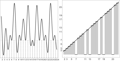
Figure 1: On the left the graphic of the Pruitt function $f_{3}$ on $D=[1.5,25.5]$. On the right, the graphic of the step map $\Psi_{3}$ with the line $y=x$ (dashed).

Let us consider $k=3$ and the Pruitt function $f_{3}$:

$$f_{3}(x)=\sin(x\,\pi/2)\,\sin(x\,\pi/3)\,\sin(x\,\pi/5),\qquad x\in I_{3}=[2-1/2,25+1/3].$$

The system Mathematica [23] has been used to compute the step map $\Psi_{3}$ defined in (16). For this prupose, the built-in system function $Round[\,]$ was used as the closest integer function.

The graphics of $f_{3}$ and $\Psi_{3}$ are displayed in Figure 1. Projecting the graph of $\Psi_{3}$ onto the $y$-axis we obtain the zeros of $f_{3}$. In fact, as predicted by Proposition 3, this set is ${\cal Z}={\cal P}_{0}\cup{\cal M}$, with

$${\cal P}_{0}=\{2,3,5\},\quad{\cal M}=\{4,6,8,9,10,12,14,15,16,18,20,21,22,24,25\},$$ (17)

where ${\cal P}_{0}$ is the set of the first $3$ primes and ${\cal M}$ the set of composite numbers which are multiples of the primes in ${\cal P}_{0}$. Moreover, by Proposition 3-(iii), the step map $\Psi_{3}$ may also be used to detect the prime numbers greater than $5$. Its clear from the graphics of $\Psi_{3}$ in Figure 1, that these prime numbers are the integers (in the $x$-axis) which belong to those intervals where $\Psi_{3}$ is equal to zero. These primes are in the set ${\cal P}=\{7,11,13,17,19,23\}$.

Remark 1.

The sieve of Eratosthenes is an algorithm providing the prime numbers less than a given integer $n\geq 2$. One of the versions of this algorithm computes precisely the set of primes ${\cal P}$ from the set ${\cal P}_{0}\cup{\cal M}$ in Proposition 3. Thus, the step function (16) may be seen as another computational version of the Eratosthenes algorithm. We refer to [12] for a discussion of efficient practical versions of the sieve of Eratosthenes using appropriate data structures.

Halley and Newton quasi-step maps for Pruitt functions

In the examples below we illustrate the construction of Halley and Newton quasi-step maps, educated by the predicates $\mathbb{P}_{0}$ and $\mathbb{P}_{1}$, for the Pruitt family. Although such construction does not depend on an a priori knowledge of the multiplicity of the zeros of the function, we note that for a Pruitt function $f_{k}$ we are dealing with both simple and multiple zeros in the interval $I_{k}$. In fact, the multiplicity of the zeros of $f_{k}$ satisfy an interesting property: on $I_{k}$ there are zeros of multiplicity $m$, where $m$ takes all the integer values $m=1,2,\ldots,k-1$. This property follows from the particular form of $f_{k}$, and although it can be proved in full generality we briefly explain it through a particular example, namely with the Pruitt function $f_{4}$.

The set of the first four primes is ${\cal P}_{4}=\{2,3,5,7\}$. Let ${\cal M}_{1}$ be the set of all the multiples of the elements of ${\cal P}_{4}$ which belong to the interval $I_{4}=[4-1/2,49+1/3]$. That is,

$$\begin{array}[]{ll}{\cal M}_{1}&=\{2,3,4,5,6,7,8,9,10,12,14,15,16,18,20,21,22,24,\\ &\hskip 14.22636pt25,26,27,28,30,32,33,34,35,36,38,39,40,42,44,45,46,48,49\}.\end{array}$$

The elements of ${\cal M}_{1}$ are zeros of $f_{4}$ having multiplicity at least one. Consider now the $6=\binom{4}{2}$ numbers which are products of two elements of ${\cal P}_{4}$. These products are

$$s_{1}=2\times 3,\,s_{2}=2\times 5,\,s_{3}=2\times 7,\,s_{4}=3\times 5,\,s_{5}=3\times 7,\,s_{6}=5\times 7.$$

Let ${\cal M}_{2}$ be the set of the multiples of $s_{1}$, $s_{2},\ldots,s_{6}$ which belong to $I_{4}$:

$$\begin{array}[]{ll}{\cal M}_{2}&=\{6,10,12,14,15,18,20,21,24,28,30,35,36,40,42,45,48\}.\end{array}$$

The elements of ${\cal M}_{2}$ are zeros of $f_{4}$ with multiplicity at least two. Thus, the simple zeros of $f_{4}$ belong to the set ${\cal Z}_{1}={\cal M}_{1}\verb+\+{\cal M}_{2}$, namely to

$${\cal Z}_{1}=\{2,3,4,5,7,8,9,16,22,25,26,27,32,33,34,38,39,44,46,49\}.$$

Taking the products of three elements of ${\cal P}_{4}$ we obtain

$$s_{1}=2\times 3\times 5,\,s_{2}=2\times 3\times 7,\,s_{3}=2\times 5\times 7,\,s_{4}=3\times 5\times 7.$$

The set ${\cal M}_{3}$ of all the multiples of $s_{1}$ to $s_{4}$ belonging to $I_{4}$ is

$$\begin{array}[]{l}{\cal M}_{3}=\{s_{1},s_{2}\}=\{30,42\}.\end{array}$$

As all the elements of ${\cal M}_{3}$ have multiplicity greater or equal to three, then ${\cal Z}_{2}={\cal M}_{2}\setminus{\cal M}_{3}$ is the set of double zeros of $f_{4}$:

$${\cal Z}_{2}=\{6,10,12,14,15,18,20,21,24,28,35,36,40,45,48\}\;\text{(double zeros)}$$

Finally, as the product of all the elements of ${\cal P}_{4}$ is $2\times 3\times 5\times 7>49$, there are not zeros of multiplicity greater or equal to four in $I_{4}$. This means that

$${\cal Z}_{3}={\cal M}_{3}=\{30,42\}\,\,\mbox{(triple zeros)},$$

is the set of the zeros of $f_{4}$ with multiplicity $m=3$ in the interval $I_{4}$.

Note that for the function $f_{3}$ treated in Example 1, either using the previous reasoning or just by the analysis of the graphic of $f_{3}$ in Figure 1, we draw the following conclusions:

• The set of simple zeros of $f_{3}$ is:

  $$\{2,3,4,5,8,9,14,16,21,22,25\}.$$ (18)

• The set of double zeros of $f_{3}$ is:

  $$\{6,10,12,15,18,20,24\}.$$ (19)

The following two examples illustrate several features of the Halley and Newton quasi-step maps, associated to Pruitt functions, educated by the predicates $\mathbb{P}_{0}$ and $\mathbb{P}_{1}$ in (3) and (4) respectively. A quasi-step map educated by the predicate $\mathbb{P}_{0}$ will be denoted by $\widetilde{\Psi}_{0}$ and by $\widetilde{\Psi}_{1}$ in the case of $\mathbb{P}_{1}$.

Example 2.

(Halley quasi-step maps for $f_{3}$)

Let $f_{3}$ be the 3th Pruitt function restricted to the interval $D=[1.5,8.5]$ and $g={\cal H}_{f_{3}}$ the respective Halley map. Let $\widetilde{\Psi}_{0}$ be a Halley map educated by the predicate $\mathbb{P}_{0}$.

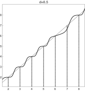
Figure 2: The Halley educated map $\widetilde{\Psi}_{0}$ for $d=0.5$ and $D=[1.5,8.5]$.

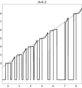
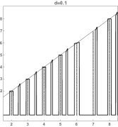
Figure 3: (A) Left, the Halley educated map $\widetilde{\Psi}_{0}$ for $d=0.2$;(B) Right, the Halley educated map $\widetilde{\Psi}_{0}$ for $d=0.1$.

Recall, from (18) and (19), that in $D$ all the zeros of $f_{3}$ are simple except $z=6$ which is a double zero. So, $2,3,4,5,8$ are super attracting fixed points of ${\cal H}_{f_{3}}$ while $z=6$ is only attracting. Between two consecutive zeros of $f_{3}$ there is exactly one repelling fixed point of ${\cal H}_{f_{3}}$. This means that ${\cal H}_{f_{3}}$ has fixed points which are not roots of $f_{3}(x)=0$. Moreover, the fixed points of ${\cal H}_{f_{3}}$ which are zeros of $f_{3}$ are precisely the attracting fixed points of ${\cal H}_{f_{3}}$ as it can be observed in Figure 2. The resolution of the set of the attracting fixed points of ${\cal H}_{f_{3}}$ is $\eta=1$. By Proposition 1, if a vertical displacement $d$ is chosen such that $d<\eta/2=0.5$, then $\widetilde{\Psi}_{0}$ must separate the attracting fixed points of ${\cal H}_{f_{3}}$ (i.e. the zeros of $f_{3}$) in $D$. This does not mean that $\widetilde{\Psi}_{0}$ separates all the fixed points of ${\cal H}_{f_{3}}$, as it is clear from Figure 3-(A) where the graphic of $\widetilde{\Psi}_{0}$ for $d=0.2$ shows that in the interval containing $5$ there are two fixed points of ${\cal H}_{f_{3}}$.

In Figure 2 and Figure 3-(B) we show the graphics of the quasi-step map $\widetilde{\Psi}_{0}$ obtained for the vertical displacement $d=0.5$ and $d=0.1$. We see that for $d=0.5$, the educated map $\widetilde{\Psi}_{0}$ coincides with ${\cal H}_{f_{3}}$ while for $d=0.1$ all the fixed points of ${\cal H}_{f_{3}}$ (not just the attracting fixed ones) have been separated in $D$.

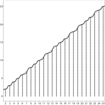
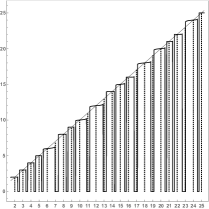
Figure 4: (A) Left the graphic of the Pruitt function $f_{3}$ in $D=[1.5,25.5]$;(B) Right the graphic of $\widetilde{\Psi}_{1}$ separating all the zeros of $f_{3}$.

We now consider $f_{3}$ defined in $D=[1.5,25.5]$ and the corresponding Halley map ${\cal H}_{f_{3}}$. As before, the graphic of ${\cal H}_{f_{3}}$ in Figure 4-(A) clearly shows the nature of the fixed points of this map. Namely, those fixed points of ${\cal H}_{f_{3}}$ that are roots of $f_{3}(x)=0$ are either acttracting or supper acttracting and the remaining fixed points are repelling fixed points. The repelling fixed points of ${\cal H}_{f_{3}}$ do not satisfy the predicate $\mathbb{P}_{1}$, since they are in contradiction with Lemma 2. Therefore, a map $\widetilde{\Psi}_{1}$, educated by $\mathbb{P}_{1}$, separates all the roots of $f_{3}(x)=0$ (cf. Proposition 2) as it is clear from the graphics of $\widetilde{\Psi}_{1}$ displayed in Figure 4-(B).

We remark that for certain classes of functions, such as the Pruitt family $f_{k}$, the corresponding Halley map enjoys the important property of continuity. This property is not verified in the case of the Newton map which will be treated in the next example. Moreover, the analysis of the graphic of ${\cal H}_{f_{3}}$ in Figure 2 confirms what is expected concerning the global convergence of Halley method, as discussed in [4], [10].

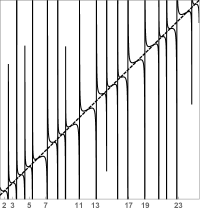
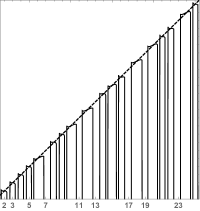
Figure 5: (A) Left, the Newton map ${\cal N}_{f_{3}}$ in $D=[1.5,25.5]$;(B) Right, the Newton educated map $\widetilde{\Psi}_{0}$, for $d=0.5$.

Example 3.

(Newton quasi-step maps for $f_{3}$)

Let us consider the Newton map ${\cal N}_{f_{3}}$ corresponding to the Pruitt function $f_{3}$ defined in $D=[1.5,25.5]$. In contrast with the Halley function of the previous example, ${\cal N}_{f_{3}}$ is not continuous in $D$ as it shows the graphic of ${\cal N}_{f_{3}}$ in Figure 5-(A). This graphic presents several vertical asymptotes which are due to the singularities of the function $f_{3}$ in the interval. However this time the fixed points of ${\cal N}_{f_{3}}$ coincide with the roots of $f_{3}(x)=0$, that is ${\cal Z}={\cal P}_{0}\cup{\cal M}$ with ${\cal P}_{0}$ and ${\cal M}$ given by (17). Obviously, the resolution of ${\cal Z}$ is $\eta=1$ and all the fixed points of ${\cal N}_{f_{3}}$ satisfy the attractivity property referred in Proposition 1. By this proposition, if one chooses a vertical displacement $d<0.5$ all the roots of $f_{3}$ will be separated by the quasi-step map $\widetilde{\Psi}_{0}$ educated by the predicate $\mathbb{P}_{0}$. The Figure 5-(B) shows that the ${\cal N}_{f_{3}}$ educated map $\widetilde{\Psi}_{0}$, for $d=0.5$, globally separates the zeros of $f_{3}$.

3.2 Quasi-step maps for a strongly oscillating function

The composition of quasi-step maps can be particularly useful to compute highly accurate roots of strongly oscillating functions as it is illustrated in the following numerical example.

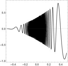
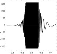
Figure 6: Left, the strongly oscillating function $f$ and right its unbounded derivative.

Example 4.

(Strongly oscillating function)

We consider the function $f(0)=0$, $f(x)=(x+1/2)^{3/2}\sin(1/x)$, for $x\neq 0$, defined in the interval $D=[-1/2,1/2]$. The function $f$ is differentiable with unbounded derivative and so it is not locally Lipschitzian. Close to the point $x=0$ the function is strongly oscillating (see Figure 6).

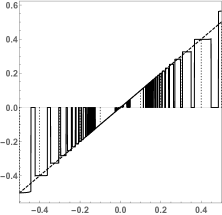
Figure 7: Halley educated maps $\widetilde{\cal H}_{f}$ (left) and $\widetilde{\cal H}^{2}_{f}$ (right).

As before, let ${\cal H}_{f}$ the Halley map associated to $f$ as defined in (14). The map $\widetilde{\cal H}_{f}$ denotes the Halley map educated by the slope predicate $\mathbb{P}_{1}$ and $\widetilde{\cal H}^{r}_{f}$ denotes its $r$-fold composition.

In Figure 7 it is displayed the graphics of the maps $\widetilde{\cal H}_{f}$ and $\widetilde{\cal H}^{2}_{f}$ which show the quasi-step nature of these maps near the endpoints of the interval. Moreover, the same figure shows that in the subinterval say $I=[-0.2,0.2]$ there is a great number of fixed points clustering around the origin.

We used the system Mathematica to compute approximations of the fixed points of $\widetilde{\cal H}_{f}$ in a certain interval centered at the origin. All the computations were carried out on a $2GHz$ Intel Core $i7$ personal computer, using standard double precision floating point arithmetic.

$$\begin{array}[]{|c|c|}\hline\cr s&\mbox{CPU time}\\ \hline\cr 2&0.38\\ \hline\cr 100&16.3\\ \hline\cr 250&40.5\\ \hline\cr 500&80.5\\ \hline\cr\end{array}$$

Table 1: CPU time (in seconds) to run $FindInstance$ to simultaneously compute a sample of $s$ roots in the interval $J=[-0.0097,0.0097]$.

Our computations were compared with those obtained by using some built-in routines of the system Mathematica. In particular, the command $Find\-Instance[expr,vars,\-Reals,s]$, with $vars$ and $expr$ assumed to be real, was used to compute an (unsorted) sample of $s$ real roots of $f(x)=0$. Notably, in the interval $J=[x_{min},x_{max}]=[-0.0097,0.0097]$ the code line $FindInstan\-ce[\{f[u]==0.,\,xmin\leq u\leq xmax\},u,s]$ was ran for several values of $s$. The respective CPU time (in seconds) is given in Table 1, which shows that for large $s$ the CPU time approximately doubles with $s$. Unless one uses the system option $WorkingPrecision$, Table 1 shows that for $s=200$ zeros of $f$ in the interval $J$, the referred time of $80.5$ seconds is quite unacceptable. In contrast, using the same default double precision computer arithmetic, the Halley educated map $\widetilde{\cal H}_{f}$ can separate, in less than one second, $s=200$ fixed points in the interval $J$.

We considered discretized versions of the maps $\widetilde{\cal H}_{f}$, $\widetilde{\cal H}^{2}_{f}$ and $\widetilde{\cal H}^{3}_{f}$ obtained by dividing the interval $J=[x_{min},x_{max}]=[-0.0097,0.0097]$ into $N=1500$ parts of length $h=(x_{max}-x_{min})/N$. The respective $N+1$ values of the maps at the points $x_{i}=x_{min}+i\,h$, with $i=0,\ldots,N$ were tabulated. Due to the large number of points considered, Table 2 only shows some of these values, namely those which are near the endpoints of $J$. For convenience, we will call $\cal T$ the full set of data obtained.

$x_{i}$	$\widetilde{\vspace{2mm}\cal H}_{f}(x_{i})$	$\widetilde{\cal H}^{2}_{f}(x_{i})$	$\widetilde{\cal H}^{3}_{f}(x_{i})$
-0.0097	-0.0097000521	-0.0097000521	-0.0097000521
-0.0096870667	-0.0096871749	-0.0096871749	-0.0096871749
-0.0096741333	-0.0096743489	-0.0096743489	-0.0096743489
-0.0096612	-0.0096615735	-0.0096615738	-0.0096615738
-0.0096482667	0	0	0
-0.0096353333	0	0	0
-0.0096224	-0.0096221501	-0.0096221501	-0.0096221501
-0.0096094667	-0.0096095803	-0.0096095803	-0.0096095803
$\qquad\cdots$	$\qquad\cdots$	$\qquad\cdots$	$\qquad\cdots$
$\qquad\cdots$	$\qquad\cdots$	$\qquad\cdots$	$\qquad\cdots$
0.0096094667	0.0096095803	0.0096095803	0.0096095803
0.0096224	0.0096221501	0.0096221501	0.0096221501
0.0096353333	0	0	0
0.0096482667	0	0	0
0.0096612	0.0096615735	0.0096615738	0.0096615738
0.0096741333	0.0096743489	0.0096743489	0.0096743489
0.0096870667	0.0096871749	0.0096871749	0.0096871749
0.0097	0.0097000521	0.0097000521	0.0097000521

Table 2: Educated maps $\widetilde{\cal H}^{r}_{f}(x)$, for $r=1,2,3$.

It is clear from Table 2 that the points $x_{i}$ where the value zero occurs for all the maps $\widetilde{\cal H}_{f}$, $\widetilde{\cal H}^{2}_{f}$ and $\widetilde{\cal H}^{3}_{f}$ provide a collection of the subintervals where the slope predicate holds true. In the full set ${\cal T}$ we found $273$ of such subintervals. In each of these subintervals there exists at least a fixed point of $\widetilde{\cal H}_{f}$. The analysis of ${\cal T}$ also shows that the maps $\widetilde{\cal H}^{3}_{f}$ and $\widetilde{\cal H}^{2}_{f}$ are numerically invariant (see also Table 2) and so all the computed nonzero values $\widetilde{\cal H}^{2}_{f}(x_{i})$ are approximations of fixed points of the Halley map ${\cal H}_{f}$, with eight significant decimal digits.

The previous procedures may be implemented in order to obtain high precision approximations of the fixed points of ${\cal H}_{f}$. This can be achieved by considering in the computations not only a convenient machine precision but also an appropriate $r$-fold composition of $\widetilde{\cal H}_{f}$. For instance, taking the same sample of 1501 points $x_{i}$ in $J$, an extended precision of 1000 decimal digits, and computing $\widetilde{\cal H}^{r}_{f}(x_{i})$, for $r=2$ to $r=5$, we obtained a new table of data in about 10 seconds of CPU time. In this case one can verifies that $\widetilde{\cal H}^{4}_{f}$ and $\widetilde{\cal H}^{5}_{f}$ are numerically invariant. In particular, for the point $x_{N-1}=0.0097-h\simeq 0.0096870667$ we have $z_{N-1}=\widetilde{\cal H}^{5}_{f}(x_{N-1})$ with

$$\begin{array}[]{ll}z_{N-1}&=0.00968717492126197578990697768061822598\\ &\hskip 113.81102pt\vdots\\ &3785734861841858811484051025080640392894,\end{array}$$ (20)

where only a certain number of the initial and the final 1000 decimal machine digits are displayed. Computing the residual $f(z_{N-1})$ we obtain

$$f(z_{N-1})\simeq 0.*10^{-997}.$$

In order to check that $z_{N-1}$ is in fact an accurate root of $f(x)=0$, we use the Mathematica function $FindRoot$ as follows:

$$\begin{array}[]{l}x_{N-1}=0.0096870667;\\ z=x\,/.\,FindRoot[f[x]==0,\{x,x_{N-1}\},\,WorkingPrecision\,->\,1000];\end{array}$$

The respective value of $z$ is such that $z-z_{N-1}\simeq 0.*10^{-1002}$ which shows that all the 1000 decimal digits of $z_{N-1}$, in (20), are correct.

As a final remark let us refer that we have applied with success several Newton and Halley educated maps to a battery of test functions suggested in [14, 2, 24, 7]. Suitable discretized versions of the respective quasi-step maps enable the computation of high accurate roots regardless these roots are simple or multiple, and so the approach seems to be particularly useful, in particular for the global separation of zeros of strongly oscillating functions.

References

- [1] S. Amat, S. Busquier, J. M. Gutiérrez, Geometric constructions of iterative functions to solve nonlinear equations, J. Comput. Appl. Math. 157 (2003), 197-205.
- [2] C. Chun, H. ju Bae, B. Neta, New families of nonlinear third-order solvers for finding multiple roots, Comput. Math. Appl. 57 (2009), 1574-1582.
- [3] R. Crandall, C. Pomerance, Prime Numbers: A Computational Perspective, Springer, 2005.
- [4] M. Davies, B. Dawson, On the global convergence of Halley’s iteration formula, Numer. Math. 24 (1975), 133-135.
- [5] P. Deuflhard, A short history of Newton’s method, Documenta Math., Extra volume ISMP (2012), 25-30.
- [6] P. Deuflhard, Newton Methods for Nonlinear Problems, Affine Invariance and Adaptative Algorithms, Springer, 2004.
- [7] A. Galántai, J. Abaffy, Always convergent iteration methods for nonlinear equations of Lipschitz functions, Numer. Alg. 69 (2015), 443-453.
- [8] M. M. Graça, P. M. Lima, Root finding by high order iterative methods based on quadratures, Appl. Math. Comput. 264 (2015), 466-482.
- [9] E. Halley, A new, exact and easy method of finding the roots of equations generally, and that without any previous reduction, Phil. Trans. Roy. Soc. London 18 (1694), 136-145.
- [10] M. A. Hernández, M. A. Salanova, Indices of convexity and concavity. Application to Halley method, Appl. Math. Comput. 103 (1999), 27-49.
- [11] J. L. Lagrange, Traité de la résolution des équations numériques de tous les degrés. Paris, 1808 ib.1826. (Available at http://dx.doi.org/10.3931/e-rara-4825).
- [12] M. E. O’Neill, The genuine sieve of Eratosthenes, J. Funct. Prog. 19 (2009), 95-106.
- [13] A. Melman, Geometry and convergence of Euler’s and Halley’s methods, SIAM Rev. 4 (1997), 728-735.
- [14] D. Nerinckx, A. Haegemans A comparison of non-linear equation solvers, J. Comput. Appl. Math. 2, No. 2 (1976), 145-148.
- [15] J. L. Nikolajsen, New stopping criteria for iterative root finding, R. Soc. open sci. (2014), 1:140206.
- [16] A. M. Ostrowski, Solution of Equations in Euclidean and Banach Spaces, Academic Press, 1973.
- [17] R. S. Palais, A simple proof of the Banach contraction principle, J. Fixed Point Theory Appl. 2 (2007), 221-223.
- [18] P. D. Proinov, S. I. Ivanov, On the convergence of Halley’s method for multiple polynomial zeros, Mediterr. J. Math. 12 (2015), 555-572.
- [19] C. D. Pruitt, Formulae for determining primality or compositeness, in http://www.mathematical.com/mathprimetest.html (unknown date).
- [20] J. F. Traub, Iterative methods for the solution of equations, Prentice-Hall, Englewood Cliffs, N. J., 1964.
- [21] J. Verbeke, R. Cools, The Newton-Raphson method, In. J. Math. Educ. Sci. Technol. 26, No. 2 (1995), 177-193.
- [22] X. Wang, P. Tang, An iteration method with maximal order based on standard information, Int. J. Comp. Math. 87 (2010), 414-424.
- [23] S. Wolfram, The Mathematica Book, Wolfram Media, fifth ed., 2003.
- [24] X. Wu, Improved Muller method and bisection method with global and asymptotic superlinear convergence of both point and interval for solving nonlinear equations, Appl. Math. Comput. 166 (2005), 299-311.
- [25] T. Yamamoto, Historical developments in convergence analysis for Newton’s and Newton-like methods, J. Comput. Appl. Math. 124 (2000), 1-23.
- [26] E. Zeidler, Nonlinear Functional Analysis and its Applications, Springer, New York, 1986.