Mass spectroscopy using Borici-Creutz fermion on 2D lattice

Abstract

Minimally doubled fermion proposed by Creutz and Borici is a promising chiral fermion formulation on lattice. In this work, we present excited state mass spectroscopy for the meson bound states in Gross-Neveu model using Borici-Creutz fermion. We also evaluate the effective fermion mass as a function of coupling constant which shows a chiral phase transition at strong coupling. The lowest lying meson in 2-dimensional QED is also obtained using Borici-Creutz fermion.

I Introduction

Chiral fermion formulation is always a challenging task on lattice and minimally doubled fermions in recent times have drawn attention as promising lattice formulations of chiral fermion. KarstenK and WilczekW proposed one formulation of minimally doubled fermion and another was developed by Creutzcreutz and Boriciborici . Both the formulations break the hypercubic symmetry on the lattice bedaque and thus allow non-covariant counter terms. The important question is how bad the effects of the symmetry breaking are in a numerical simulation. It was shown that a consistent renormalizable theory for minimally doubled fermion can be constructed by fixing only three counter terms allowed by the symmetry and the counter terms for BC action at one loop in perturbation theory have been evaluated capitani1 ; capitani2 . But, till date, sufficient numerical studies of the minimally doubled fermions have not been done. The purpose of this work is to investigate Borici-Creutz(BC) formulation numerically in some models.
The BC fermion formulation was motivated by the fact that electrons on graphene lattice are described by a massless quasi-relativistic Dirac equation. The BC fermion describes two chiral modes or the two flavors of chiral fermion located at $(0,0,0,0)$ and at $(\frac{\pi}{2},\frac{\pi}{2},\frac{\pi}{2},\frac{\pi}{2})$. It was shown that in presence of gauge background with integer-valued topological charge, BC action satisfies the Atiyah-Singer index theoremdc . In GCB , using BC fermion we have shown a chiral phase transition in the Gross-Neveu model. We extend that investigation further in this work to meson spectroscopy of the Gross-Neveu model as well as in 2D QED (QED₂) using BC fermion. Chiral and parity-broken(Aoki) phase structures of the Gross-Neveu model have been studied for Wilson and Karsten-Wilczek fermions CKM ; misumi . A lattice simulation of the Gross-Neveu model using the Wilson fermion was done by Korzec et alkorzec , where the recovery of chirally invariant Gross-Neveu model from a lattice model was studied. The semimetal-insulator phase transition on a graphene lattice with Thirring type four fermion interactions has been studied by Hands and collaboratorshands and the strong coupling analysis of the tight-binding graphene model with Kekule distortion term has been done by Arakiaraki . We use pseudofermion HMC for lattice simulation of the Gross-Neveu model. The feasibility of psedofermion algorithm in the Gross-Neveu model has been studied by Campostrini et. al.Camp .

In this paper, we perform hybrid Monte Carlo(HMC) simulation to investigate the excited state spectrum of the lattice Gross-Neveu model. Extraction of the excited state spectrum is always a difficult task on lattice. As of now, variational method gives the best spectrum. From the slope of the correlators, we first obtain some preliminary estimate about the masses and then we use variational method to extract the meson masses. Excited state spectroscopy in the Gross-Neveu model with Wilson fermion has been studied in Danzer , where the authors obtained the ground state as the only bound state and the other excited states were scattering states. With the BC fermion, we have obtained three states, two of them are bound states (ground state and one excited state) and the third one appears to be a scattering state. We also evaluate the fermion mass in the model which shows that it is consistent with a chiral phase transition at large coupling observed in GCB . Next we investigate the meson mass spectrum in QED in two dimension. QED₂ having confinement has bound state spectrum and serves as a toy model for hadronic bound states in QCD. In continuum, massless Schwinger model is exactly solvable and can be represtented as a free boson theory. QED₂ or Schwinger model has been studied to great extent on lattice (see Gutsfeld ; Gattringer and references therein). Schwinger model using Hamiltonian formalism on lattice has been investigated in cichy . QED₂ also serves as a good toy model for numerical study of chiral fermions. A 2-flavor Schwinger model with light fermions have been studied with dynamical overlap fermion Giusti ; Hip . Here, we study the model with the minimally doubled fermion, namely, the BC fermion.

II Spectroscopy of the Gross-Neveu model

The free BC action in 2D is written as,

$$S = \sum_{n}\left[\frac{1}{2}\sum_{\mu}\overline{\psi}_{n}\gamma_{\mu}(\psi_{n+\mu}-\psi_{n-\mu})-\frac{ir}{2}\sum_{\mu}\overline{\psi}_{n}(\Gamma-\gamma_{\mu})(2\psi_{n}-\psi_{n+\mu}-\psi_{n-\mu})\right.$$ (1)

$$\left.-i(2-c_{3})\overline{\psi}_{n}\Gamma\psi_{n}+m_{0}\overline{\psi}_{n}\psi_{n}\right],$$

where, $\mu=1,2$ and $\Gamma=\frac{1}{2}(\gamma_{1}+\gamma_{2})$ satisfies $\{\Gamma,\gamma_{\mu}\}=1$. Including four-fermion interactions, the Gross-Neveu model with a discrete $\gamma_{5}$ symmetry on lattice is given by

$$S = \sum_{n}\left[\frac{1}{2}\sum_{\mu}\overline{\psi}_{n}\gamma_{\mu}(\psi_{n+\mu}-\psi_{n-\mu})-\frac{ir}{2}\sum_{\mu}\overline{\psi}_{n}(\Gamma-\gamma_{\mu})(2\psi_{n}-\psi_{n+\mu}-\psi_{n-\mu})\right.$$ (2)

$$\left.-i(2-c_{3})\overline{\psi}_{n}\Gamma\psi_{n}+m_{0}\overline{\psi}_{n}\psi_{n}-\frac{g^{2}}{2N}[(\overline{\psi}_{n}\psi_{n})^{2}+(\overline{\psi}_{n}i\Gamma\psi_{n})^{2}\right],$$

where, $g$ is the coupling constant which we consider the same for both scalar and vector four point interactions and we set $r=1$ in our calculations. Since the parity is broken by the BC action, a counter term $c_{3}$ is added to it. Detailed discussion about the $c_{3}$-term can be found in GCB . Now, the action is rewritten explicitly in terms of the auxiliary fields as

$$S=\sum_{m,n}\overline{\psi}_{m}M_{mn}\psi_{n}+{\frac{N}{2g^{2}}}(\sigma^{2}+\pi_{\Gamma}^{2}),$$ (3)

where $N$ is the number of flavors. The auxiliary fields

$$\sigma=-\frac{g^{2}}{N}(\overline{\psi}\psi),$$

$$\pi_{\Gamma}=-\frac{g^{2}}{N}(\overline{\psi}i\Gamma\psi)$$ (4)

are defined in the dual lattice sites $\tilde{l}$ surrounding the direct lattice site $l$ hands2 .

$$M_{mn}=D_{mn}+\frac{1}{4}\sum_{\langle l,\tilde{l}\rangle}{(\sigma(\tilde{l})+i\pi_{\Gamma}(\tilde{l})\Gamma)},$$ (5)

where $\langle l,\tilde{l}\rangle$ denotes four dual lattice sites $\tilde{l}$ surrounding the direct lattice site $l$ and $D_{mn}$ is the BC Dirac operator:

$$D_{mn} = \frac{1}{2}\gamma_{\mu}(\delta_{n,m+\mu}-\delta_{n,m-\mu})+\frac{i}{2}(\Gamma-\gamma_{\mu})(\delta_{n,m+\mu}+\delta_{n,m-\mu})$$ (6)

$$~{}~{}~{}-((2-c_{3})i\Gamma-m_{0})\delta_{m,n}.$$

Since $M$ is a complex matrix, we work with (${M}^{\dagger}M$) to make it real and positive definite and integrate out the fermion fields by the pseudofermion method. Since the Borici-Creutz action describes two flavors, the number of flavors becomes double i.e., $N_{f}=2N=4$ for an action with ($M^{\dagger}M$). In 2D, counter terms can be tuned to restore Lorentz invariant dispersion relation and here we can set the dimension two counterterm to zero; Lorentz symmetry can be controlled by $c_{3}$ alone. The minimally doubled fermions have physical dispersion relation for $0<c_{3}<0.59$ and $3.41<c_{3}<4$ and the two chiral phase boundaries are near $c_{3}=0$ and $c_{3}=4$ GCB . For the mass spectroscopy, we consider here $c_{3}=0.1$ i.e., in the minimal double region with Lorentz invariant dispersion relation and reasonably away from the phase boundaries. The value of $c_{3}$ is not completely arbitrary, other values of $c_{3}$ in the minimally double region are equally valid, the numerical values may change for different $c_{3}$, but the physics remains unchanged.

With pseudofermions the action becomes ,

$$S=\phi^{\dagger}(M^{\dagger}M)^{-1}\phi+\beta(\sigma^{2}+\pi_{\Gamma}^{2}),$$ (7)

where, $\beta={1/{g^{2}}}$. We perform hybrid Monte Carlo(HMC) simulation using this lattice action. The configurations are generated by considering step-size($\triangle{t}$)=0.1 in the leapfrog method and ten steps per trajectory in the molecular dynamics chain. We do not use any preconditioning during the simulation. First 1000 ensembles are rejected for thermalization and analysis is performed over the next 8000 ensembles.

II.1 Correlators

For meson mass spectrum calculation, we need to evaluate the correlators

$$C_{ij}(t)=\langle O_{i}(t)O_{j}^{\dagger}(0)\rangle.$$ (8)

Since we cannot have orbital angular momentum in 2D, the interpolators ($O_{i}$) are labelled by parity and charge conjugation only. It is important to choose the appropriate operators which have good overlaps with the low lying states. For the meson spectroscopy, we consider only the odd parity interpolators. The even parity interpolators are not considered as they do not decay exponentially and correspond to condensatesDanzer . Since under parity $\psi(x,t)\to\gamma_{2}\psi(-x,t)$, the odd parity interpolators can be constructed with $\gamma_{1}$ or $\gamma_{5}$. Along with the local source, one can also construct the interpolators with the fields at different lattice sites shifted along the spatial direction ie., with $\psi(x\pm n,t)$ . If one considers a relative negative sign in between $\psi(x+n,t)$ and $\psi(x-n,t)$ then this corresponds to a derivative source which are found to be important for excited state spectroscopyDanzer ; Dsource . Combining the field operators at different lattice sites, many interpolators can be constructed but it was found in our numerical analysis that they mostly couple to the ground state. InDanzer , a set of nine different interpolators were listed. Here we list some of the parity odd interpolators for the GN model which we expect to couple to ground state as well as excited states:

$$O_{1}(t) = {\overline{\psi}}(x,t)\gamma_{5}\psi(x,t)$$

$$O_{2}(t) = \frac{1}{4}\big{(}({\overline{\psi}}(x+m,t)-\overline{\psi}(x-m,t)\big{)}\gamma_{5}\big{(}\psi(x+n,t)-\psi(x-n,t)\big{)},(m=3,n=3)$$

$$O_{3}(t) = \frac{1}{4}\big{(}({\overline{\psi}}(x+m,t)-\overline{\psi}(x-m,t)\big{)}\gamma_{5}\big{(}\psi(x+n,t)-\psi(x-n,t)\big{)},(m=5,n=3)$$

$$O_{4}(t) = \frac{1}{4}\big{(}({\overline{\psi}}(x+m,t)-\overline{\psi}(x-m,t)\big{)}\gamma_{1}\big{(}\psi(x+n,t)-\psi(x-n,t)\big{)},(m=4,n=3)$$

$$O_{5}(t) = \frac{1}{4}\big{(}({\overline{\psi}}(x+m,t)+\overline{\psi}(x-m,t)\big{)}\gamma_{1}\big{(}\psi(x+n,t)-\psi(x-n,t)\big{)},(m=5,n=3),$$

where sum over $x$ is implied in order to have zero momentum states and $\gamma_{5}=i\gamma_{1}\gamma_{2}$. All the interpolators are odd under $C$-parity ($C=-1$). With different values of $m$ and $n$, we can have different interpolators, but the one that are found to couple with ground state as well as the excited states are for the values listed above in Eq.(LABEL:interpol), other interpolators do not couple to new states but only reproduce the similar results.

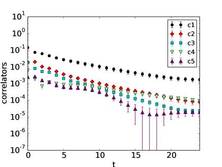
(a) (b)

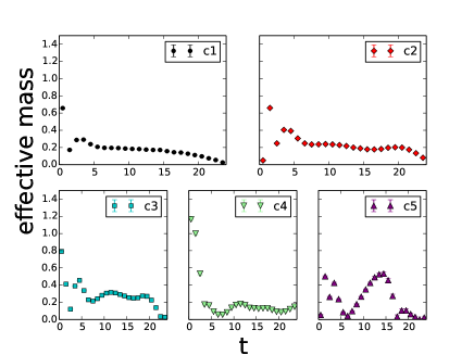
Figure 1: Diagonal correlators (in the plots $c1\equiv C_{11}$, etc.) and effective mass of meson in GN model for $16\times 48$ lattice

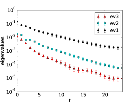
(a) (b)

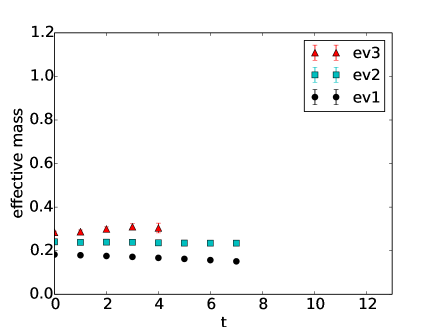
Figure 2: Eigenvalues and effective mass of the correlators for $16\times 48$ lattice

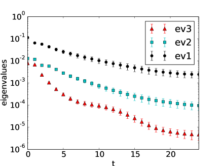
(a) (b)

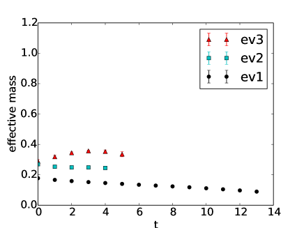
Figure 3: Eigenvalues and effective mass of the correlators for $20\times 48$ lattice

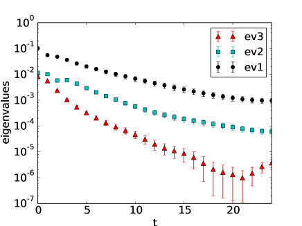
(a) (b)

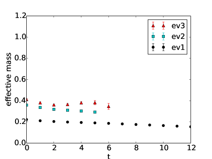
Figure 4: Eigenvalues and effective mass of the correlators for $22\times 48$ lattice

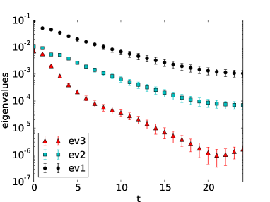
(a) (b)

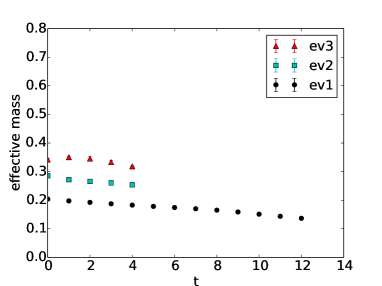
Figure 5: Eigenvalues and effective mass of the correlators for $24\times 48$ lattice

II.2 Effective mass calculation

The effective masses are extracted from the correlators at different time slices by the formula

$$M_{eff}=\ln\left(\frac{c(t)}{c(t+1)}\right).$$ (10)

The diagonal correlators $C_{ii}$ and corresponding effective masses are shown in Fig.1(a) and (b) for $m_{0}=0.03$ and $\beta=0.7$. The small value of mass is taken to be close to the massless limit. Eq.(10) is an approximate formula and found good for ground state but can also produce approximate values for the excited states. As can be seen from Fig. 1(b), except for the ground state, this procedure cannot extract the excited states well enough, we only see a hint of two other possible states. Analysis of the eigenvalue spectrum of the correlation matrix, on the other hand, provide a better picture for the meson spectroscopy. In the variational method Michael ; Luscher , to get the mass spectrum from eigenvalues one solves the generalized eigenvalue problem defined by

$$C(t)\vec{v}^{(n)}=\lambda^{(n)}(t)C(t_{0})\vec{v}^{(n)}$$ (11)

where $C(t)$ is the $N\times N$ correlation matrix constructed from $N$ interpolators $O_{i},~{}(i=1,2\cdots,N)$. The $n$-th eigenvalue behaves as

$$\lambda^{(n)}(t)=e^{-(t-t_{0})E_{n}}\Big{[}1+\mathcal{O}(e^{-(t-t_{0})\Delta_{n}})\Big{]},$$ (12)

where $E_{n}$ is the energy of the $n$-th state and $\Delta_{n}$ is the energy gap between the neighboring states. In Fig.2 we show the eigenvalue and effective mass plots by solving the generalized eigen value problem for $16\times 48$ lattice with $O_{1},~{}O_{2}$ and $O_{3}$ interpolators. We are unable to get any extra stable mass values by increasing the matrix dimension of the correlator basis. So, we work with only $O_{1},~{}O_{2}$ and $O_{3}$. The results become noisier if the matrix dimension is increased by including more correlators. We have shown the eigenvalues and effective mass plots for the $16\times 48$ lattice in Fig.2. Three mass plateau can be observed in Fig.2(b). In Fig.3 , Fig.4 and Fig.5 we have shown the eigenvalues and effective masses for $20\times 48,~{}22\times 48$ and $24\times 48$ respectively..

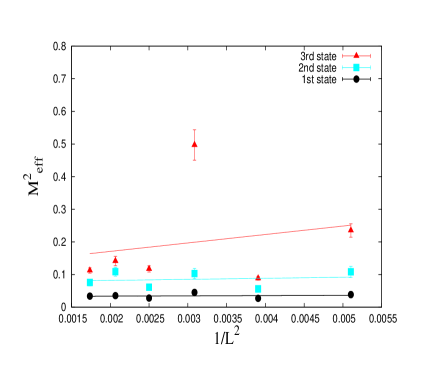
Figure 6: Volume dependence of the effective mass.

In Fig.6, the volume dependence of the effective masses are shown. The ground state and the first excited state show no volume dependence and hence can be considered as bound states. The second excited state however shows a weak volume dependence. Specially, for $18\times 48$ lattice size, we get an anomalously large mass for the second excited state. The fit for the second excited state shown in Fig.6 includes this anomalous point. In general, scattering states show strong volume dependence and increase linearly with $1/L^{2}$, the volume dependency of the second excited state in our case is not very conclusive. But looking at the fit of the points we expect it to be a scattering state. The results can be contrasted with Danzer where the Gross-Neveu model was studied with Wilson fermion. In Danzer , except the ground state, all the excited states show strong volume dependence and are scattering states. At least for Gross-Neveu model, BC fermion works better for excited state spectroscopy.

II.3 Fermion mass and chiral phase transition

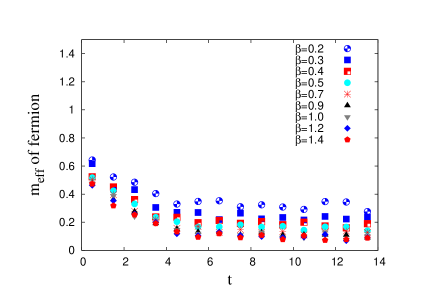
(a) (b)

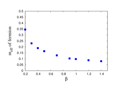
Figure 7: (a) Effective mass of the fermion in GN model, (b) the variation of effective electron mass with $\beta$ is consistent with the chiral phase transition demonstrated in Ref.GCB . The fermion bare mass is $m_{0}=0.03$.

In GN model, we have also extracted the effective mass of the fermion. For the fermion mass calculation, we consider the correlator with $O(t)=\psi(x,t)$ and evaluate the effective fermion mass for different values of the coupling constant $\beta$. The effective masses for different $\beta$ are shown in Fig.7(a). We take $c_{3}=0.0001$ to be close to the phase boundary. Fig. 7(b) shows the variation of effective electron mass with the coupling constant. At small $\beta$( i.e., at large coupling), the electron mass rapidly increases indicating a phase transition as can be seen from Fig. 7(b). In GCB , it was shown with Borici-Creutz fermion that the GN model with a discrete chiral symmetry shows a second order chiral phase transition at $\beta\approx 0.4$. The current result for the $\beta$-dependence of the electron mass is consistent with that finding. The systematics of the continuum limit are not studied here.

III Meson in 2D QED

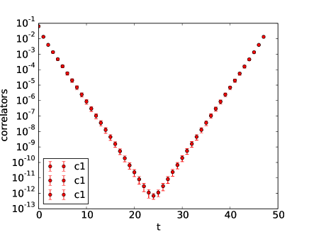
(a) (b)

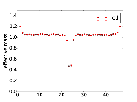
Figure 8: Effective mass of meson in 2D QED for $m_{0}=0.05$ and $\beta=0.3$.

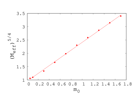
Figure 9: Fermion mass dependence of the effective pion mass in QED₂ for a fixed $\beta=0.3$.

In this section, we extend the study of spectroscopy with BC fermion formulation to gauge theory. For this purpose, we implement the BC fermion in a 2D $U(1)$ gauge theory and extract the meson masses. QED in 2D is also a confined theory and serves as a good toy model for QCD. The Gross-Neveu model, having a discrete chiral symmetry, undergoes spontaneous breaking but in the massless Schwinger model the chiral symmetry is continuous and cannot be spontaneously broken. The lattice action with BC fermion reads,

$$S=\beta\sum_{p}[1-\frac{1}{2}(U_{p}+U^{\dagger}_{p})]+\phi^{\dagger}(D^{\dagger}D)^{-1}\phi.$$ (13)

where $U_{p}$ is the Wilson Plaquette action with

$$U_{p}=U_{i,\mu}U_{i+\mu,\nu}U^{\dagger}_{i+\nu,\nu}U^{\dagger}_{i,\nu}.$$ (14)

where, $i$ is the site index and $\mu,\nu$ are the directions and $D$ is the BC Dirac operator defined in eqn.(6). After including gauge fields we get,

$$D_{mn} = \frac{1}{2}(\gamma_{\mu}+i(\Gamma-\gamma_{\mu}))U_{\mu}(n-\mu)\delta_{n,m+\mu}-$$ (15)

$$\frac{1}{2}(\gamma_{\mu}-i(\Gamma-\gamma_{\mu}))U^{\dagger}_{\mu}(n)\delta_{n,m-\mu}-((2-c_{3})i\Gamma-m_{0})\delta_{m,n}.$$

Here we concentrate only for the lowest lying meson mass. The correlator with operator $O_{1}(t)$ couples to the ground state and provides the mass for the lowest state which we call pion following the general convention. In Fig.8(a) we have shown the correlator at different time slices and the effective meson mass in 2D QED. The results are presented for the fermion (electron) mass $m_{0}=0.05$ and $\beta=0.3$. The effective pion mass is shown in Fig.8(b). The Schwinger model in continuum can be written as a bosonic theory. The pion mass in the bosonized theory can be exactly calculatedsmilga and for $m_{0}\ll g$, can be written as

$$M_{eff} = A~{}m_{0}^{N_{f}/(N_{f}+1)}g^{1/(N_{f}+1)}=A~{}m_{0}^{5/4}g^{1/5}~{}~{}\rm{(for~{}N_{f}=4)},$$

$$= A~{}m_{0}^{4/5}\beta^{-1/10}$$

where $A$ is a constant and $\beta=1/g^{2}$. In Fig.9, we show the fermion mass dependence of the effective pion mass ($M_{eff}^{5/4}\propto m_{0}$). The plot is done for small $\beta$ so that $m_{0}$ is always less than $g$. The lattice data are in well agreement with the analytic result.

IV Summary

Minimally doubled fermions may provide an efficient lattice formalism to study chiral fermion which is expected to be computationally cheaper than the other existing lattice formalisms. Since, both the minimally doubled fermion formulations (KW and BC) break hypercubic symmetries on the lattice, they require non-covariant counter terms. Only detailed numerical studies can confirm how bad or manageable its effects are on the lattice, and whether any meaningful computation is possible with minimally doubled fermion or not. In this work, we have studied the BC fermion in some simple models. We have extracted the excited state mass spectrum in Gross-Neveu model using BC fermion. The absence of volume dependence of the first two states suggests that they are mesonic bound states and the third state show a weak volume dependence. The effective fermion mass has also been evaluated as a function of the coupling constant $\beta$. It shows a phase transition consistent with the result obtained in GCB . We have also evaluated the lowest lying meson mass in QED₂. The lattice results are consistent with the prediction from analytic calculation in the bosonized model. Our investigations suggest that BC fermion formalism might be a promising alternative to study the chiral fermions on a lattice. One obviously needs more detailed numerical study in 4D gauge theory with dynamical BC fermion to confirm that claim. Invesigation of BC fermion in 4D QCD in a mixed-action lattice simulation is in progress.

References

- (1) L.H. Karsten, Phys. Lett. B 104,315 (1981).
- (2) F. Wilczek, Phys. Rev. Lett. 59,2397 (1987).
- (3) M. Creutz, JHEP 0804, 017(2008); Pos LAT2008, 080 (2008).
- (4) A. Borici, Phys. rev. D. 78, 074504 (2008).
- (5) P. F. Bedaque, M. I. Buchoff, B.C. Tiburzi, A. Walker-Loud, Phys. Lett. B. 662,449 (2008).
- (6) S. Capitani, J. Weber, H. Wittig, Phys. Lett. B681, 105 (2009).
- (7) S. Capitani, M. Creutz, J. Weber, H. Wittig, JHEP 1009, 027 (2010).
- (8) D. Chakrabarti, S. J. Hands, A. Rago, JHEP 0906, 060 (2009).
- (9) J. Goswami, D. Chakrabarti and S. Basak, Phys. Rev. D 91, no. 1, 014507 (2015).
- (10) M. Creutz, T. Kimura, T. Misumi, Phys. Rev. D.83, 094506 (2011).
- (11) T. Misumi, JHEP 1208, 068 (2012).
- (12) T. Korzec, F. Knechtli, U. Wolff, B. Leder, PoS LAT2005, 267 (2006).
- (13) S. J. Hands, C. Strouthos, Phys. Rev. B78, 165423 (2008), W. Armour, S. Hands, C. Strouthos, Phys. Rev. B81, 125105(2010).
- (14) Y. Araki, PoS LAT2011, 054 (2011); Phys. Rev B 85, 125436 (2012).
- (15) M. Campostrini, G. Curci and P. P. Rossi, Nucl. Phys. B 314, 467 (1989).
- (16) J. Danzer and C. Gattringer, PoS LAT 2007, 092 (2007).
- (17) C. Gutsfeld, H. A. Kastrup and K. Stergios, Nucl. Phys. B 560, 431 (1999).
- (18) C. Gattringer, I. Hip, C. B. Lang, Phys. Lett. B 466,287 (1999).
- (19) K. Cichy, A. Kujawa-Cichy and M. Szyniszewski, Comput. Phys. Commun. 184, 1666 (2013).
- (20) L. Giusti, C. Hoelbling and C. Rebbi, Phys. Rev. D 64, 054501 (2001).
- (21) W. Bietenholz, I. Hip, S. Shcheredin and J. Volkholz, Eur. Phys. J. C 72, 1938 (2012).
- (22) S. J. Hands, A. Kocić, J. B. Kogut, Nucl. Phys. B390, 355 (1993), Ann. Phys. 224, 29 (1993).
- (23) C. Gattringer, L. Y. Glozman, C. B. Lang, D. Mohler and S. Prelovsek, Phys. Rev. D 78, 034501 (2008).
- (24) C. Michael, Nucl. Phys. B 259, 58 (1985).
- (25) M. Luscher and U. Wolff, Nucl. Phys. B 339, 222 (1990).
- (26) A. V. Smilga, Phys. Rev. D 55, 443 (1997).